Reliability of Extreme Significant Wave Height Estimation from Satellite Altimetry and In Situ Measurements in the Coastal Zone

Abstract

Measurements of significant wave height from satellite altimeter missions are finding increasing application in investigations of wave climate, sea state variability and trends, in particular as the means to mitigate the general sparsity of in situ measurements. However, many questions remain over the suitability of altimeter data for the representation of extreme sea states and applications in the coastal zone. In this paper, the limitations of altimeter data to estimate coastal Hs extremes (<10 km from shore) are investigated using the European Space Agency Sea State Climate Change Initiative L2P altimeter data v1.1 product recently released. This Sea State CCI product provides near complete global coverage and a continuous record of 28 years. It is used here together with in situ data from moored wave buoys at six sites around the coast of the United States. The limitations of estimating extreme values based on satellite data are quantified and linked to several factors including the impact of data corruption nearshore, the influence of coastline morphology and local wave climate dynamics, and the spatio-temporal sampling achieved by altimeters. The factors combine to lead to considerable underestimation of estimated Hs 10-yr return levels. Sensitivity to these factors is evaluated at specific sites, leading to recommendations about the use of satellite data to estimate extremes and their temporal evolution in coastal environments.

1. Introduction

Measurements of significant wave height (Hs) from satellite altimeter are finding increasing application in investigations of wave climate, variability and trends [1,2,3,4,5,6]. Near complete global coverage and a continuous record of 28 years makes it an attractive source of observational data. The European Space Agency (ESA) Sea State Climate Change Initiative (CCI) project [6] recently released version 1.1 of their satellite altimeter data product, comprising both along-track 1 Hz measurements (Level 2P, L2P [7]) and multi-mission gridded maps of significant wave height (Level 4, L4 [8]). This carefully quality controlled and calibrated data product provides new opportunities to examine long-term variability of Hs across most of the globe. However, important questions remain over the suitability of these data for certain applications, notably extreme sea state estimation and coastal applications.

Understanding long term variability in the extremes of sea state is clearly a high priority noting the vulnerability of coastal communities and marine industry [9,10,11]. A key challenge for extremes remains the availability of long term observational data. Moored data buoys typically offer the most reliable long term time series of sea state variables but these records are sparse and unevenly distributed. Hemer [12], for example, proposes estimates derived from the only known long-term buoy record exposed to the long-fetch Southern Ocean wave conditions. Research is further hampered by the fact that buoys may carry a range of instrumentation that responds differently to wave conditions—particularly the extremes [13]—and whose operational maintenance is generally not driven by long term climatological considerations, suffering frequently from changes in instrument types, changing calibration practices and platform refits through their lifetimes [14]. Noting these challenges, researchers find strong incentives in exploiting nearly 3 decades of remotely sensed data, that provide regular observations over much of the world’s oceans. This is particularly attractive in remote parts of the ocean, or less developed regions where in situ infrastructure is lacking. Accurate satellite observations may offer a superior alternative to the use of simulated or hindcast model datasets that are often used in their absence. Meucci et al. [15] find that the heterogeneous assimilation rates of satellite observations into reanalyses can introduce spurious temporal wind speed and wave height trends.

Given the availability of these high quality long term satellite records of sea state, recent efforts have attempted to identify long term trends in mean wave conditions (Hs) [3] and in extremes [4,16]. But while the accuracy of altimeter sea state measurements can be good enough when extreme conditions are experienced, the statistical estimation of extremes is subject to the spatio-temporal sampling associated with particular geographical locations, their proximity to satellite ground tracks and the number of altimeters flying at any given time. Changes in the number of concurrent missions (which has increased steadily over time) and their changing orbit configurations have led to high variability in available sampling on inter-annual timescales, with strong spatial heterogeneity. One method used to overcome these sampling issues is to aggregate sea state data over larger areas, typically of order $2^{\circ }$ (∼200 km) e.g., [16]. However, the suitability of such aggregation is subject to the spatial scales of variability of the underlying wave climate and aggregation at several 100 km may not be appropriate or informative where wave climate changes over short distances, such as coastal regions. At the global scale, Jiang [4] describes in some detail the issues arising due to low altimeter sampling rates and explores several methods of mitigation, ultimately advocating for a hybrid approach that relies on the combined use of altimetry and reanalysis data. Ideally, a spatial statistical model for extremes can be used, to account for and exploit such spatial variations. But the application of these advanced methods typically rely on having adequate temporal sampling at a number of dependent locations [5,17,18]. Where this is not possible, such as in the case of low temporal sampling altimeters attempting to capture fast-varying storms, it remains unclear to what extent such methods can be routinely applied in the case of waves.

Aside from potential sampling deficiencies, altimeter wave height measurements, including extremes, in the open ocean are typically of good accuracy [1,6], but within a few kilometers from shore, altimeter signals can be contaminated by the presence of nearby land, leading to large data dropout or loss of accuracy. Many studies have examined the performance of altimeter measurements of Hs in coastal regions [19,20,21]. In recent years, coastal altimetry re-tracking algorithms have been developed to mitigate these effects near land and retrieve more and better altimeter data in coastal regions. Within the ESA Sea State CCI project, competing coastal re-tracking algorithms were evaluated against a range of criteria for implementation in future versions of the Sea State CCI product. Schlembach et al. [21] describe this “round-robin” process in detail, noting that while improvements over operational re-tracking algorithms were widely obtained, the exact performance improvements between algorithms was strongly sensitive to proximity to the coast (see also [22]). While such efforts focus on the detailed performance of altimetry measurements they do not necessarily provide insight into their overall limitations when employing a larger combined dataset, such as the Sea State CCI product, across a range of coastal regions and conditions. While the study by Jiang [4] goes a long way towards explaining the nature and impact of altimeter under-sampling for the Hs distribution and trends on the global scale (typically working at a $2^{\circ }\times 2^{\circ }$ grid), there is something of an absence of research with a focus on specific regions and applications, including the coastal zone. Key questions in this context therefore include: to what extent does infrequent sampling impact analyses of extremes offshore; how does proximity to the coast further reduce data integrity and; how does that reduction—and its impact on extremal analyses—vary as a function of geographic location.

In this paper we explore these questions with the use of satellite altimeter Hs data in the ESA Sea State CCI L2P product. We examine sampling characteristics in a number of regions around the U.S. with different wave climate, considering pairs of sites located nearshore (no less than 5 km from the coast) and offshore (up to 330 km). We characterise the considerable sampling variability both spatially (with distance to coast) and temporally over the period of the satellite era (1992 to 2018). Standard matchup and statistical comparisons confirm the good agreement between satellite and buoy measurements of Hs, including in the extremes. But, commensurate with other results [4], the low temporal sampling frequency leads to considerable underestimation of extremes in coastal regions. It is clear from our results that nearshore, the low temporal sampling problem of altimetry is exacerbated by data loss due to land contamination, and that there is considerable sensitivity to a range of factors primarily driven by geographic location.

The structure of this paper is therefore as follows. Section 2 describes the regions of study and the data sources used, together with a summary of the statistical methods applied. This is followed by Section 3 that describes the results, including summaries of overall sampling characteristics by region, summaries of agreement between the buoy and satellite data and the impact of under-sampling on long period return level estimates. Discussion of salient points is presented in Section 4 and finally we summarise with some brief conclusions in Section 5.

2. Data Sources and Methods

2.1. Geographic Choices and Data Sources

In order to understand the representation of coastal wave climate and extremes from satellite measurements, we inter-compare the data and analyses in pairs of nearshore and offshore locations in relatively close proximity to each other on the global scale. We use long term in situ observations in both nearshore and offshore settings as benchmarks of the true wave climate and extremes at those sites. In this way it is possible to identify deficiencies of the satellite measurements offshore—where coastal effects have no influence—and establish how those deficiencies (if any) are affected with distance to the coast. Long term in situ records of Hs are fairly sparsely available, and even more so nearer to the coast. Here we have used measurements from the moored data buoys maintained by the National Oceanographic Data Center (NODC) shown in Figure 1. We focus on a range of geographic sites located close to the United States east and west coasts, and including the Gulf of Mexico. For inshore/offshore pairs, to a good approximation both locations are influenced by a common large scale wave climate that, to some extent, reduces inter-site discrepancy due to geographic difference. Subsequent analyses therefore show a truer representation of the difference due to sampling rather than site-dependent wave climate and characteristics. Our choice of nearshore sites is limited to a minimum distance of approximately 5 km from the coast, owing to the limited availability of data from moored buoys. Geographic regions containing a nearshore/offshore pair of buoys are numbered #1 to #6 and are indicated by blue boxes in Figure 1, together with the distance to the coast noted in the legend.

Measurements of Hs from these data buoys span more than 10 years, and typically cover most of the period of continuous satellite coverage (1992 to present, see Figure 1). Sampling frequency is typically hourly but occasionally differs between buoys. Predominantly our analysis is based upon 1-h averaged values. Although it is known that the continuity and stability of data from buoys can be affected by physical and operational impacts, such as change in payload (see e.g., [14]) we do not account for such impacts here.

2.2. Observations from Satellite Altimetry

Measurements of Hs inferred from satellite altimetry are taken from the recently released ESA CCI Sea State L2P product [6,7]. It provides calibrated and quality controlled 1 Hz along-track observations from 10 satellite missions (provided separately) including: ERS-1, TOPEX/Poseidon, ERS-2, GFO, Envisat, Jason-1, Jason-2, Cryosat-2, Jason-3 and SARAL/Altika (note SENTINEL-3 missions A and B are not included). Throughout this paper the calibrated 1 Hz along-track measurements are compared with in situ observations at fixed locations by aggregation and averaging over a 50 km radius, chosen in accordance with common convention [22]. We acknowledge that evaluation over smaller scales might well be desirable for some applications, for example leading to closer correlation to point observations (from buoys), but this typically leads to impractical levels of sampling and is particularly problematic for the analysis of extremes. This issue is discussed further in Section 4.2.

Given the satellite ground speed along the orbit, 1 Hz sampling leads to approximately one measurement every 7 km along-track at sea level, and the possibility of multiple track segments from different satellites within the (typical) radius of 50 km separation. For detailed time series analysis (see e.g., Section 3.2), we take averages over 1-h bins. Consistent with the processing for the Sea State CCI Level 4 dataset, and others (e.g., [4]), we typically take a median of each track segment. In (rare) cases, where more than one track segment lies within a 1-h bin, in order to avoid statistical biases associated with weighting heavily in favour of track segments that happen to have a much larger number of points, we take the mean of the median values. Note also that conventionally where specific buoy and satellite measurement “match ups” are identified for precise calibration (e.g., [22]), a time window of 30 min is adopted. In this case however we are working with long time series that makes this impractical. Furthermore, typically buoy sampling frequency is limited to 1 h so little additional resolution can be gained.

As part of the Sea State CCI L2P product, the 1 Hz data points are associated with a considerable amount of additional information, including data quality flagging for each measurement. Further details are provided in the Product User Guide [23]. Of primary importance is the quality flag, “qual_flag” which takes integer values from 0 to 3, where the value of 3 corresponds to “Good” data and is what we have generally exploited in this study. In addition, a “Rejection Flag” is also provided. Its value is based on a binary decomposition that corresponds to one or more reasons for the rejection of “Good” quality. That is, one observation can be associated with more than one reason for rejection. While we do not examine in detail data where qual_flag < 3, we note that a value of 2 typically denotes data affected by sea-ice, a value of 1 (corresponding to “Poor” data) denotes data affected by other factors, and a value of 0 indicates a missing Hs measurement. Note that flagging observations as “Good” quality generally implies a value of zero for the rejection flag. That is, as one might expect, there is no reason to reject good quality data. However, one exception to this is that nearly all (>99%) of the ERS-1 and ERS-2 data flagged as good (qual_flag = 3), is also designated with a non-zero rejection flag value. This indicates a problem with “waveform_validity” in the vast majority of instances. Nonetheless, in spite of this, we have indeed found the data to be of good quality (in accordance with qual_flag = 3), and there does not appear to be any reason to doubt the integrity of the ERS-1 and ERS-2 data. This data has therefore been retained in our analysis. A detailed explanation and investigation of the use of rejection flags is complex and beyond the scope of this study, but further information can be found in the Product User Guide [23] and mission specific literature. Rejection flag designations are listed in the legends of Figure 2 and Figure 3 and some specific examples of rejection flags offshore are provided in Figure 7a. Further information about their frequency of usage in the coastal zone is discussed in Section 3.1 and Section 4.1.

2.3. Statistical Comparisons and Extreme Value Analysis

In Section 3.2, standard statistical approaches are employed in order to assess the consistency between satellite and in situ data.

In addition, in Section 3.3, Hs extremes are evaluated more explicitly. Our objective is to examine the effect of satellite under-sampling on estimation of extreme Hs. “Return levels” express the expected maximum value of a variable after some specific time, and are commonly used as a measure of extreme in analyses and engineering assessments. We evaluate the Hs 10-year return level (the maximum value of Hs expected to occur within 10-years) using an extreme value modeling approach. Specifically we use generalized extreme value models fitted using a block-maxima (annual) sampling approach, from which the 10-year return level can be easily inferred [24,25]. Note that while it is common to consider much longer return periods in engineering applications (e.g., 50 to 100 years), the 10-year return level is chosen to avoid additional uncertainty introduced by the limited duration of available data. The complete available 1-h averaged Hs time series from a number of buoys are used as source data. An extreme value model is fitted to these annual maxima. Although this approach is commonly employed in the literature, and we have found the 10-year return levels consistent with the long term records, we do not emphasise claims here about their accuracy. More detailed modeling refinements could certainly be explored. For example, in this approach we apply statistical models with no temporal dependence and we do not explicitly consider seasonality. While inter-annual variability from different sources is likely to be an important factor, the objective is to quantify the effect of under-sampling, rather than to obtain an accurate estimate of return level using complex techniques. To that end, 10-year return levels are estimated from reduced data sets by iteratively sub-sampling each year from the complete record at a range of percentage levels between 1% and 100% (per year) of the total available data. Note that years in the buoy record with <75% availability were discarded. For each of the iterations, a new series of annual maxima are generated, from which an estimate of the 10-year return level (and its 95% confidence bounds) can be made. For each percentage level, samples were drawn randomly from each year based on a uniform probability distribution, with 500 iterations (at each percentage level). The 10-year return level and confidence interval was computed at each iteration from the sub-sampled time series, and finally mean values were obtained. We note that 500 iterations was somewhat conservative since mean values were found to converge after far fewer iterations. The Hs 10-year return levels associated with the reduced samples can be compared with the sampling levels typically seen for the satellites in order to understand, approximately, the nature and scale of the inaccuracy one might expect when using the satellite data in isolation.

3. Results

In Section 3.1 we show details of how the abundance and quality of the 1 Hz measurements are affected by distance to the coast, and how the various satellite missions comprising the Sea State CCI L2P dataset contribute to sampling throughout the available temporal record at the locations identified in Figure 1. In Section 3.2 hourly time series from data buoys and satellite are examined in more detail to reveal agreement in the extremes. Finally, the impact of under-sampling on 10-year return level estimation is explored and quantified in Section 3.3. Note that due to practical considerations we show only a limited number of results in the main manuscript. Additional figures are provided in the supplementary information.

3.1. Regional Sampling Variation

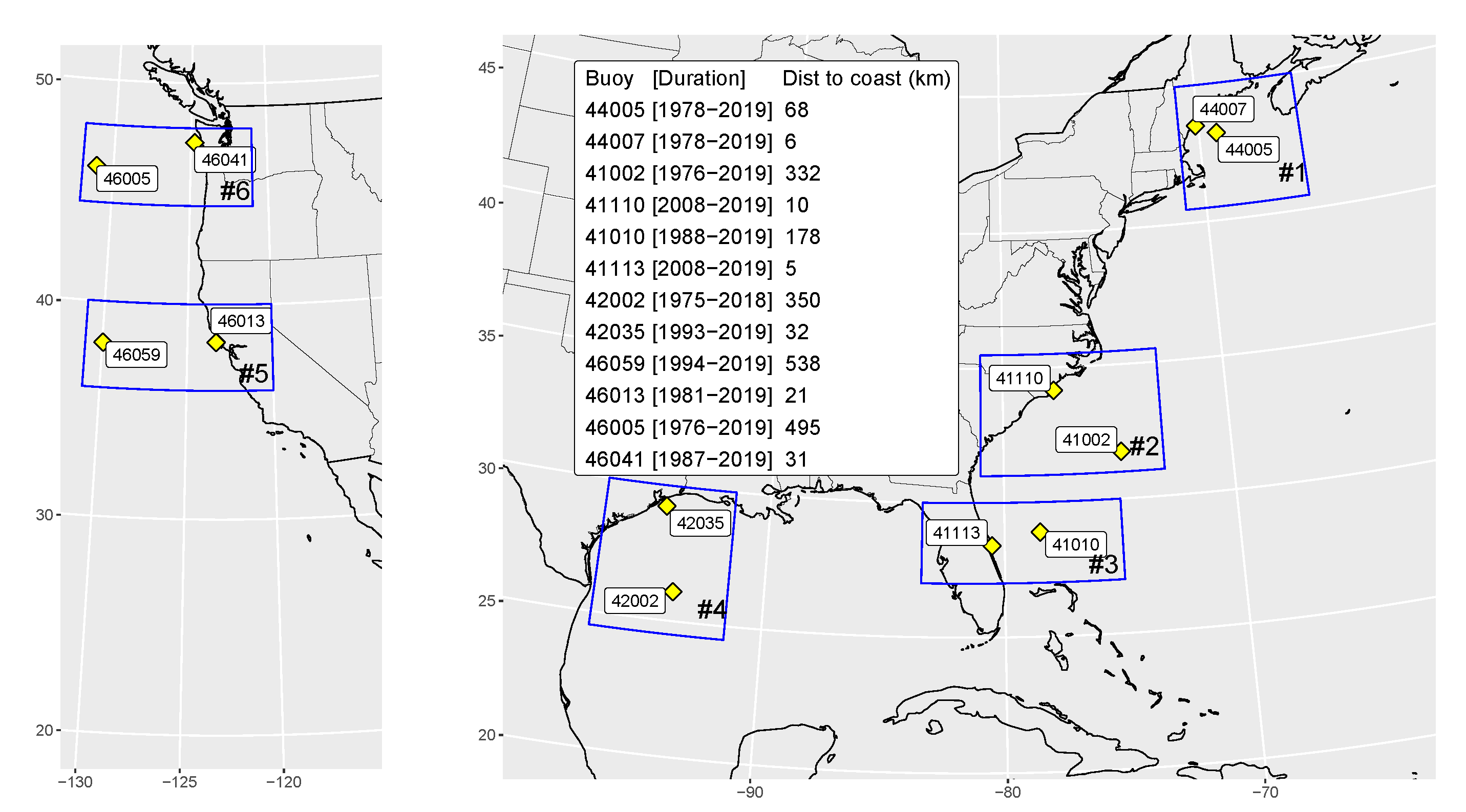
Understanding of the quality of the sea state observations is an essential part of any data analysis, providing an insight into altimeter performance close to the coast and offshore. This is particularly important for interpreting the results of extreme analyses where sampling of rare (extreme) events can be problematic. Thus, we investigate both the quality of the data (for all missions) as a function of distance to the coast, and the annual sampling characteristics of data within a 50 km radius of the buoy. 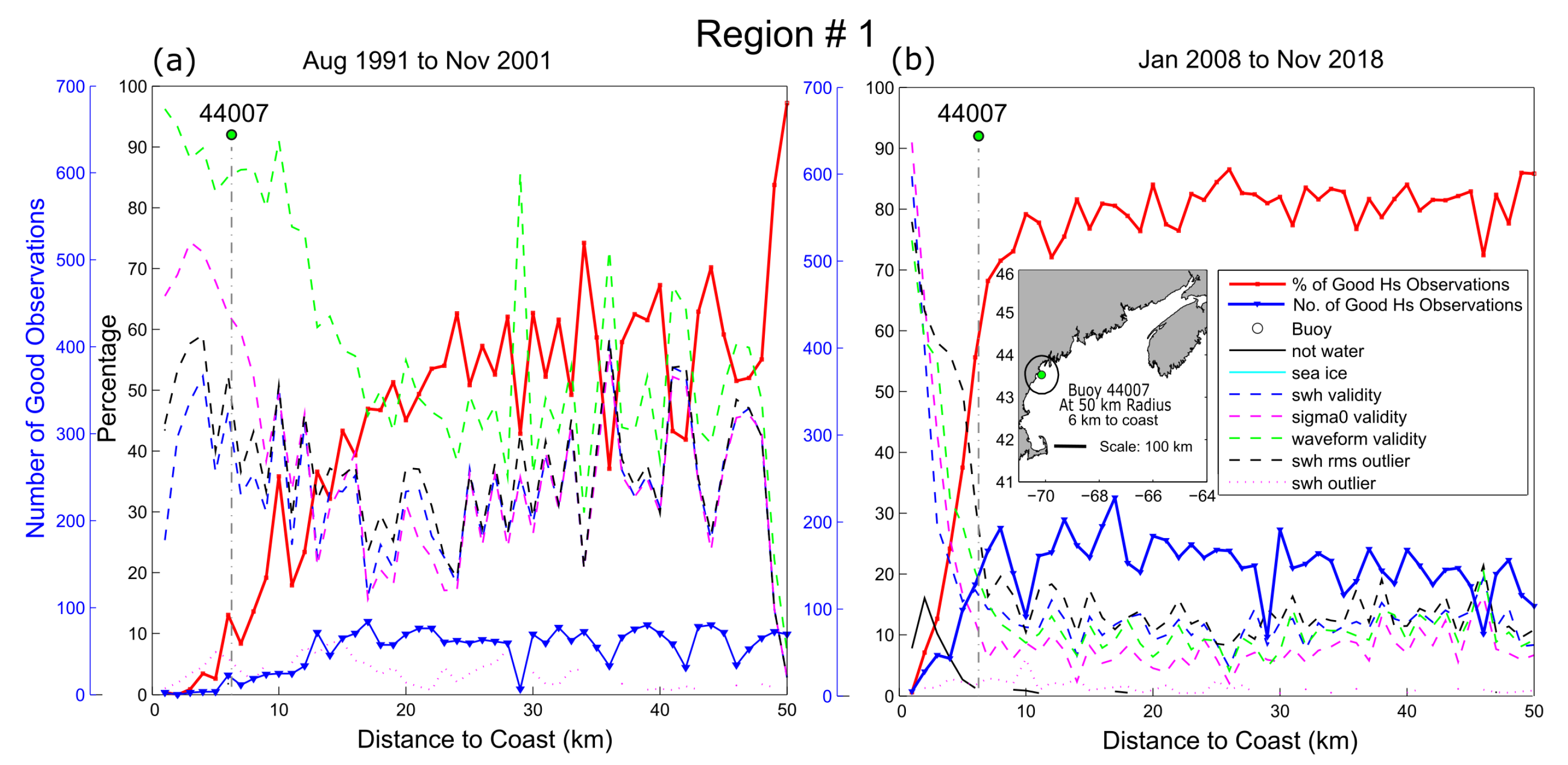The six regions (see Figure 1) representing the positions of pairs of buoys are examined. The distance of the nearshore buoy is marked on the figures for reference. The sampling characteristics with distance to the coast for region #1 are shown in Figure 2. We focus primarily on the “Good” data (qual_flag = 3, solid blue and red lines). Be aware that the total number of observations, and their distribution with distance to coast, is a function of our circular sampling area which itself depends on the exact position of the buoy in question. Therefore comparisons between regions should be made carefully, but we advise that the percentage of good data (solid red line) is a more site independent measure in this regard. We calculate the distance to the coast by applying the “great-circle” distance based on the high resolution dataset, Global Self-consistent Hierarchical High-resolution Geography, GSHHG [26]. The high resolution GSHHG dataset is about an 80% reduction in size and quality compared with the original (full) data resolution of 0.1 km ${}^2$ (https://www.soest.hawaii.edu/pwessel/gshhg/).

There is a marked difference in data quality and abundance in the first decade of the record (Figure 2a) compared with the most recent decade (Figure 2b). In particular, the total number of good data points (solid blue line) is substantially lower in the first period but good data also represents a much lower percentage of the total data (solid red line). While this percentage rises with increasing distance to the coast, it remains below 40% up to 20 km and remains around 50% thereafter. This contrasts considerably with more recent years where, at even less than 10 km to the coast, good data exceeds 50% and is typically closer to 80%. The proportions of data associated with rejection flags are also shown (dotted and dashed lines) and these clearly correspond to the remaining data that is not marked as “Good” (qual_flag = 1, 2). Note that more than one rejection flag may be assigned to a single measurement. Approaching the coast the “waveform_validity” flag (green dotted line) appears to be the dominant flag but this is far more pronounced in the earlier part of the record (panel a). While we do not describe in detail the causes for the designation of rejection flags, we note that they are somewhat mission specific and inference for their application requires a thorough case-by-case examination that we do not conduct here.

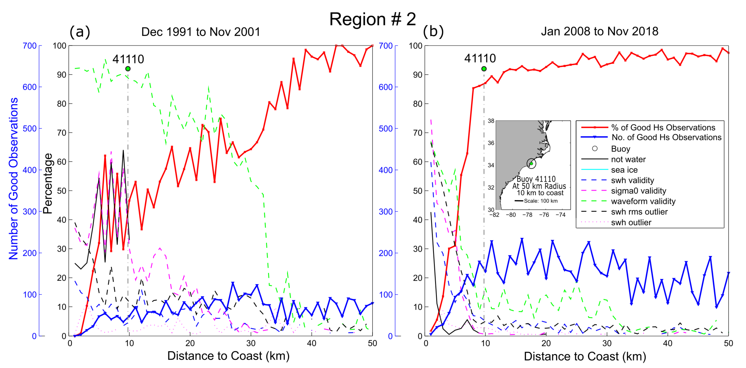
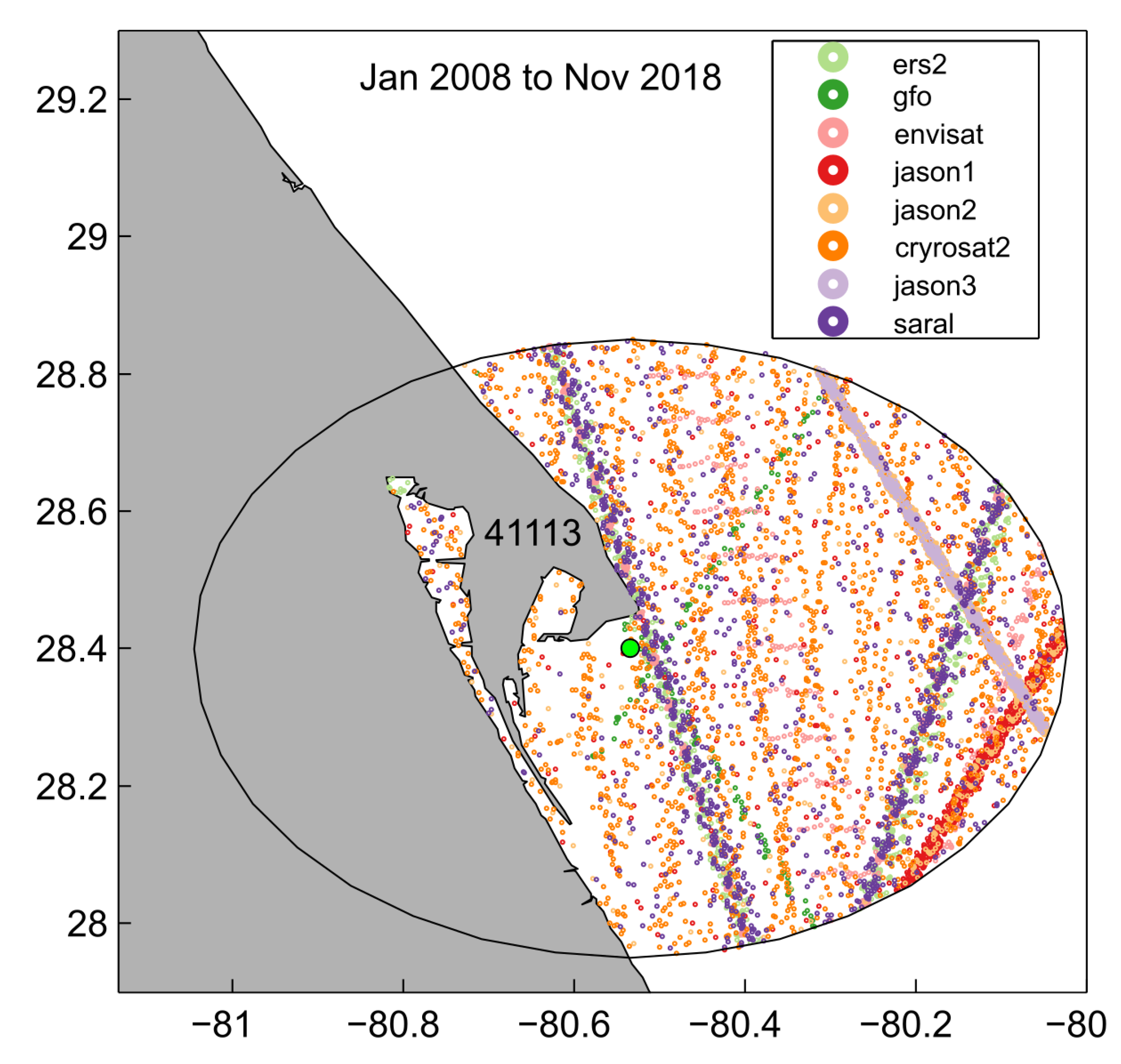
The overall general pattern, with an increase in total observations and a considerable improvement in good data percentage in more recent years, applies to all other regions (#2 to #6, Figure 3 and Figures S1,S3,S5 and S7). This phenomenon clearly corresponds to the changes in missions from fewer earlier spacecraft and instruments with typically lower reliability, to more numerous and higher quality platforms more recently. Across all regions however, there is an enormous amount of variability in data quality and rejection flagging with distance to the coast. This arises due to different combinations of satellite track that happen to intersect the particular location. In region #3 (U.S. east coast, near buoy 41113, Figure S1), for example, a large increase in observations is seen at approximately 35 km. This likely corresponds to an orbital track from a specific mission. A close examination of the satellite tracks contributing to this data in the latter decade, shown in Figure 4, suggests this is likely attributable to a combination of Jason-1, Jason-2 and Jason-3 and SARAL.

The unique and varied properties of different geographic locations are a function of many variables. Firstly, owing to the orbital paths of the spacecraft, sampling density increases at higher latitudes. As a result, at lower latitudes, there is a higher probability that a given site (of the same spatial extent) will not intersect the path of a given mission. Conversely, some sights may lie close to the intersection of tracks from multiple missions that then provide an abundance of observations. As can be seen in some locations (see e.g., Figures S1 and S7), numbers of observations can vary by over an order of magnitude with both distance to coast and sampling period. Note also that altimeters may occasionally change orbits, change instrument mode and go on- or off-line at various times.

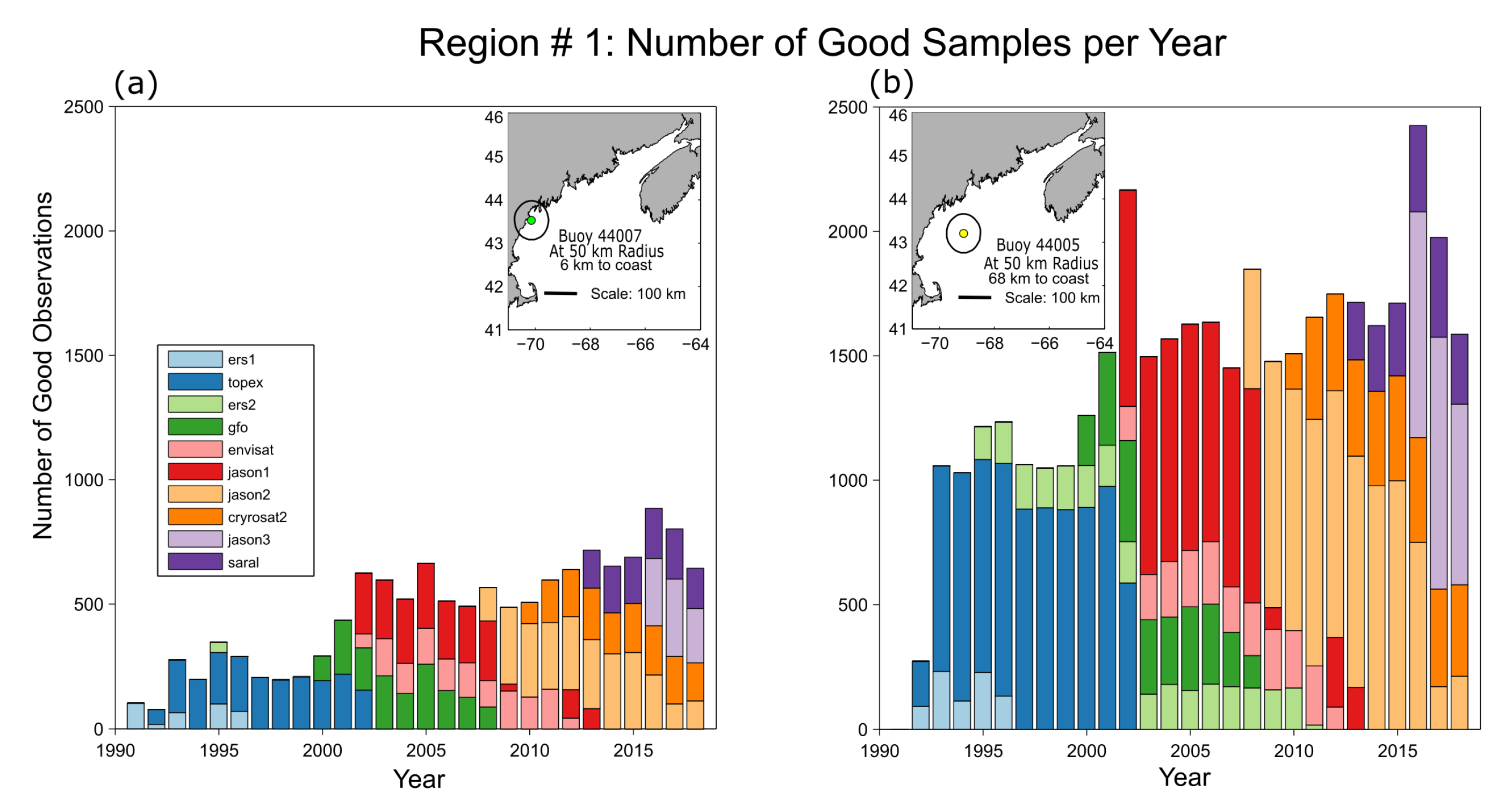
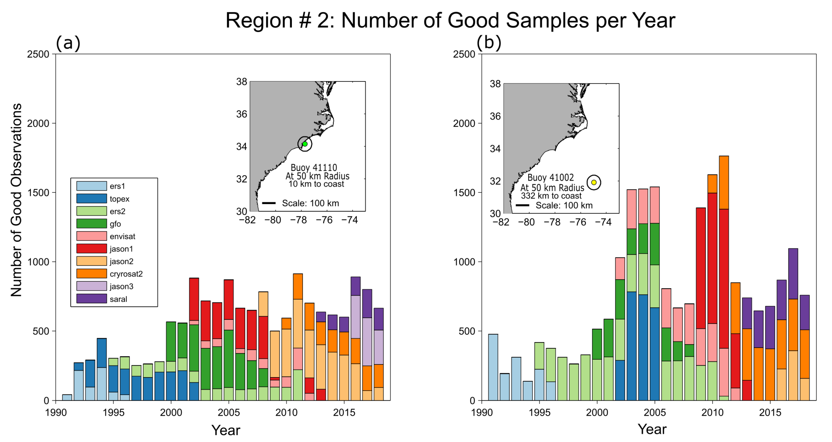
Detailed temporal properties of altimeter sampling is of interest and variability in total annual “Good” Hs measurements by mission is shown for the various buoy locations in regions #1 and #2 in Figure 5 and Figure 6 respectively. The coloured bars that correspond to the different missions that contribute measurements clearly show the missions entering and leaving service. However, there is substantial variability even where the same missions contribute to successive years. In both regions (#1 and #2), there is a clear increase in data at the offshore buoy location largely due to the fact that the sampling radius (50 km) is not partially over the land as is the case for the nearshore location. While this is somewhat obvious, in fact it raises questions about how the ocean surface area, should or could, be geographically sampled and aggregated when focusing on the nearshore. Clearly if a buoy is being used for calibration, then employing a fixed radius around the buoy is somewhat incompatible with the requirement for data being equidistant from the coast. Decisions regarding sample aggregation are likely to be needed on a case-by-case basis, and this is discussed further in Section 4.2. Nonetheless, in this case although the land removes approximately 50% of the sampling area nearshore (Figure 5a), the increase in data seen offshore (Figure 5b) is only partially accounted for by the increase in sampling area. The additional data loss nearshore is explained by the increase in rejected data seen in e.g., Figure 2 with approach to the coast. However, remarkably, in region #6 (Figure S8a), although the nearshore sampling area is partially over land, more observations are available than the corresponding buoy offshore (Figure S8b) for the entire record.

The heterogeneity in inter-annual sampling of good data is in fact remarkable, all the more so since it is a strong function of location. For example, within 50 km of buoy 41002 (Figure 6b) in the western Atlantic (∼330 km offshore), TOPEX/Poseidon and the Jason missions are largely missing from the record and only contribute data during their corresponding satellite orbit interleave modes. This can be compared with Figure 5b where Jason-2 (marked in pale orange) was the majority contributor between 2009 and 2016. In addition, at buoy 41002 (Figure 6b), inter-annual variation sometimes exceeds 100% with notable increases in sampling around 2005 and 2010. In particular the average difference between the periods 1991 to 1999, and 2003 to 2005 is approximately a factor of 3. Similar patterns are seen at the other sites (see Figures S2, S4, S6 and S8), together with large variability in annual sampling as a function of location.

In summary, this overview of the data reveals the substantial heterogeneity in sampling both temporally and with distance to the coast when exploiting the Sea State CCI L2P dataset. This sampling variation itself is also highly sensitive to location which motivates considerable caution where small scale analyses are desirable for specific applications. While this cannot be linked to impacts on extreme analysis directly (which we examine in more detail in Section 3.2 and Section 3.3), any analysis (including extremes) of variability will be profoundly sensitive to location and impacted by loss of good quality data approaching the coast, particularly in early parts of the record where, in some locations, good data is virtually absent. The assessment of long term temporal trends, particularly within 50 km of the coast, must therefore be treated with caution and considered carefully on a case-by-case basis.

3.2. Representation of Extremes

Results in Section 3.1 reveal the extent of the loss of sampling of satellite observations when approaching the coast, the heterogeneity in inter-annual sampling rates and the sensitivity of these factors to geographic location. While it is clear that sampling rates can be low and variable, such information does not support a quantitative assessment of the impact on the estimation of extremes. Even with low sampling rates, it is important to establish, for example, whether observations made nearer the coast accurately capture extreme events, and whether this is dependent upon mission.

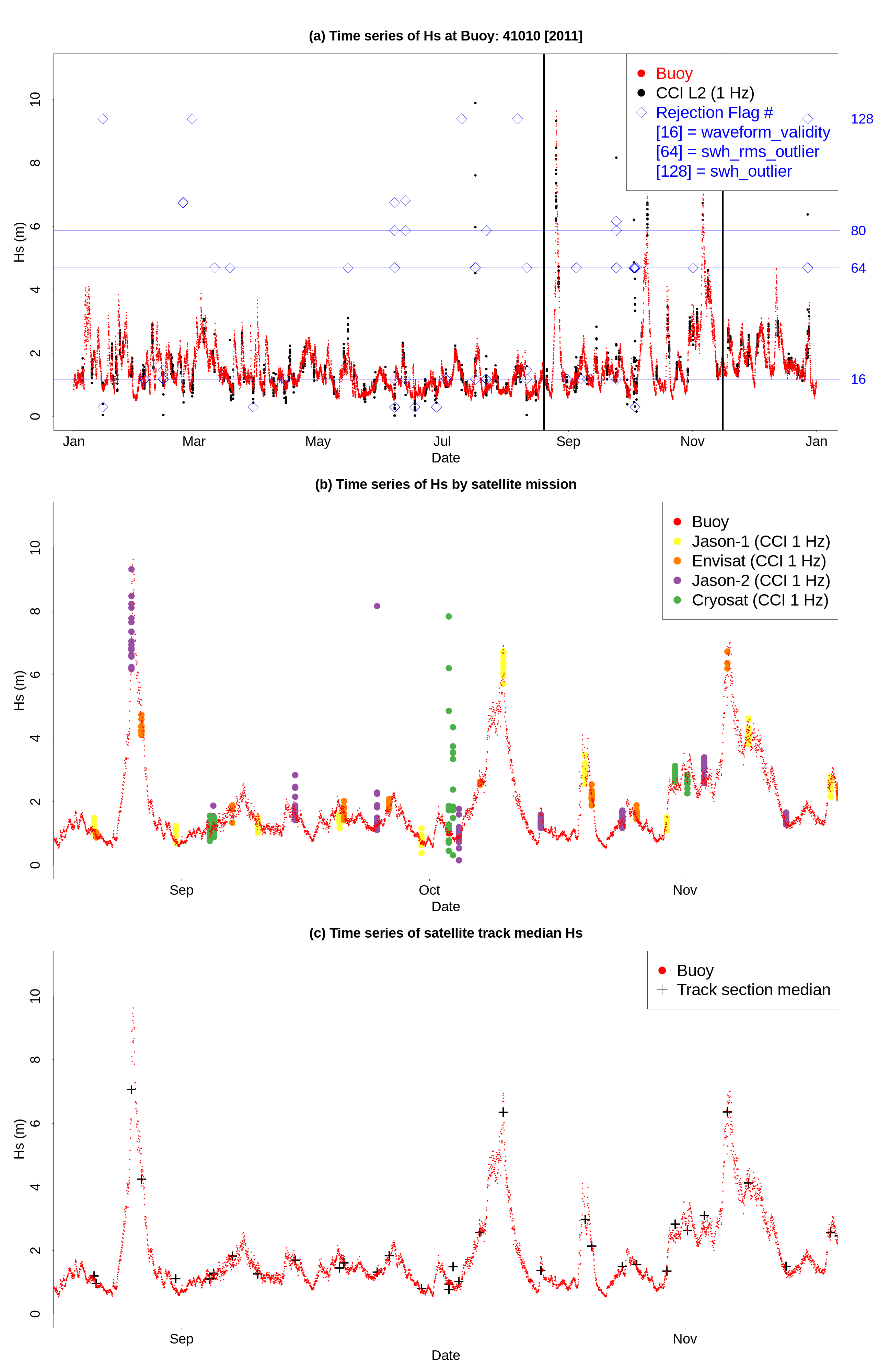
A comparison of a short time series from a buoy and the Sea State CCI L2P product is shown in Figure 7. The series of hourly measurements of Hs acquired at buoy 41010 during 2011 (red points, all panels) is overlaid by 1 Hz measurements acquired from all satellite missions observing a region of radius 50 km around the buoy location. The choice of this buoy as an example is somewhat arbitrary although in part is due to the passage of high intensity storms, including two major hurricanes (Irene and Ophelia), making it a useful example in the context of extremes. A total of four different missions were flying concurrently during this particular period and how they each contributed to this data can be seen in Figure 7b.

In panel (a), all 1 Hz measurements (black dots) are overlaid. The scatter of the 1 Hz measurements is readily apparent and clustering occurs since several point measurements are made during each pass. Since the number of 1 Hz measurements varies in each pass, it is typical to take a median value of Hs of the track section that intersects the area of interest. Such an approach is shown in panel (c). In spite of the scatter, we can see that generally the satellite measurements coincide well with buoy and although they are sporadic (characterised by their orbital paths), frequency of passage is fairly homogeneous. In particular we draw attention to the period between the two solid vertical black lines in Figure 7a. This part of the time series can be seen in more detail in panels (b) and (c), discussed shortly. Three particularly energetic storms passed fairly close to buoy 41010 during this time, the closet being hurricane Irene. Jason-2 was passing just before the peak of the storm and captured values of Hs at around 7 m. (Note that the highest value captured (around 9 m) does not coincide precisely with the storm peak, being a little earlier, and so was somewhat overestimated, probably due to the energetic sea state at the time).

In addition to the Hs observations, non-zero valued rejection flags associated with each 1 Hz observation are also shown (blue diamonds) in Figure 7a. The value scale for these flags is provided on the y axis on the right-hand side and indicated by horizontal blue lines. The inclusion of this data provides an indication of their frequency of occurrence and how they relate to the Hs observations. Noting that buoy 41010 lies ∼178 km offshore, some spuriously low and high values of Hs are evident. While the range of rejection flags are numerous and underlying reasons for their issuance are somewhat complex, we draw attention in particular to the “swh_outlier” flag (=128). With careful scrutiny, it can be seen that while there are occurrences of this flag, it does not tend to coincide with high energy events. Or put another way, (climatologically) high values are not typically being marked as “outliers” and discarded. Indeed, the absence of any rejection flags for the most extreme events shown suggests that data quality is largely independent of the energetic magnitude of the sea state.

In Figure 7c, results were filtered by qual_flag = 3, and median values are shown for each track segment that passed through the area of 50 km radius. This approach reduces noise and is similar to that used in the generation of the Sea State CCI L4 gridded product. When presented in this way, the generally good agreement between the two sources during the most energetic events is readily visible. We note however the presence of some spurious high valued satellite data—in particular from Cryosat at the beginning of October. This data was flagged as “Poor” quality (qual_flag = 1) and hence was removed when filtered. After filtering, the corresponding median value, seen in Figure 7c, is much closer to the buoy observation. Also seen is the fairly low frequency of sampling and it is fair to assume that in this example, the coincidence of satellite passage and the extremes was reasonably fortuitous. What we can take away from this therefore is that altimetry captures the extremes accurately when passage happens to coincide with the event.

It is important to verify that agreement between buoy and satellite is good on longer time scales. Q-Q plots (see Figures S9–S14) in a number of locations show close agreement in terms of the overall climatology but given our interest in understanding the differences in the representation of extremes, such methods are insufficient. For example, it is important to understand whether (extreme) events are observed concurrently by both observation systems and if so, to what extent do they agree in magnitude. Scatter plots based upon paired hourly mean values reveal the joint structure of the two data sets.

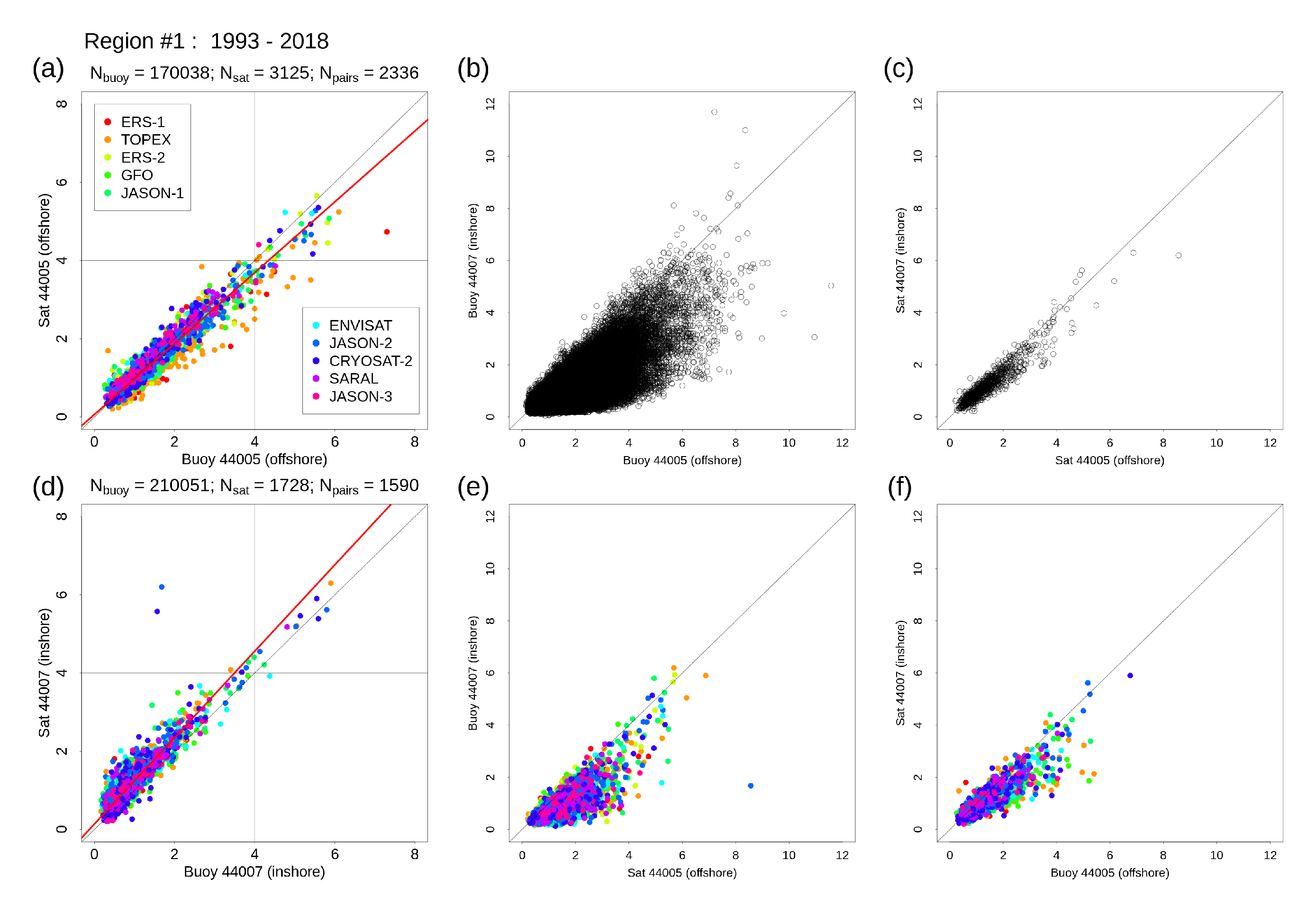
Plots for the pair of buoys (44005 and 44007) in region #1 are shown in Figure 8, for the various combinations of the offshore and nearshore data. Note that a small amount of data is unused in this approach since pairs of observations are required. Over the 26 year period a total of 170,038 h observations are available from the buoy, this compares to only 3125 (=1.8%) available in the Sea State CCI L2P product. For Figure 8a, the total number of pairwise comparisons is 2336, fewer than the total available since there is not always a corresponding value in the specific hourly slot in the opposing record. Furthermore, substantially more data pairs, and larger values of Hs, are present in Figure 8b and Figure 9b. (This is also the case for the Q-Q plots, Figures S9–S14). This is due to the fact that the buoy-buoy comparisons tend to involve near-complete 1-h time series, and so very little data, including extremes, is lost during pair-wise analyses. Figure 8a,d show the comparison between the buoy and satellite pairs for the offshore and nearshore buoys respectively. In both cases the agreement overall is good but it can also be seen in the upper right quadrants that agreement in the extremes is good. Notably, for the majority of the most extreme values nearshore, the agreement is excellent. In this example there are however three anomalous points, one offshore and two nearshore. The regression models (red lines) suggest that there is systematic bias in both cases (of different sign), but such an analysis is not appropriate for the extreme’s alone, since it is based on all the data. The general absence of points in the top left and bottom right quadrants suggests that extremes observed by the satellite are typically consistent with those observed by the buoy. We note also that there is not any clear connection between mission and observations of extremes, although some features are apparent, such as the tendency for the early missions (ERS-1, TOPEX, ERS-2) to underestimate (see Figure 8a). The four remaining panels (b,c,e,f) show the relationship between the wave climate at the different buoy locations, and how well this relationship is represented in the satellite data. Panels (b) and (c) can be compared although it is immediately clear that the relatively few pairs of points from the satellites (panel c) makes it difficult to draw robust conclusions. In fact, Figure 9c (and also Figures S15–S18) reveal an extremely low number of coincident observations. This is attributed to the fact that some buoy pairs share a direction of separation that happens to coincide with the direction of travel of one or more satellites. Thus, on a single passage, there is a high probability that the satellite will pass both buoy locations, leading to temporally coincident measurements. For buoy pairs with different spatial orientations this is not the case and coincident measurements are much rarer. This effect is further exacerbated by increased spatial separation.

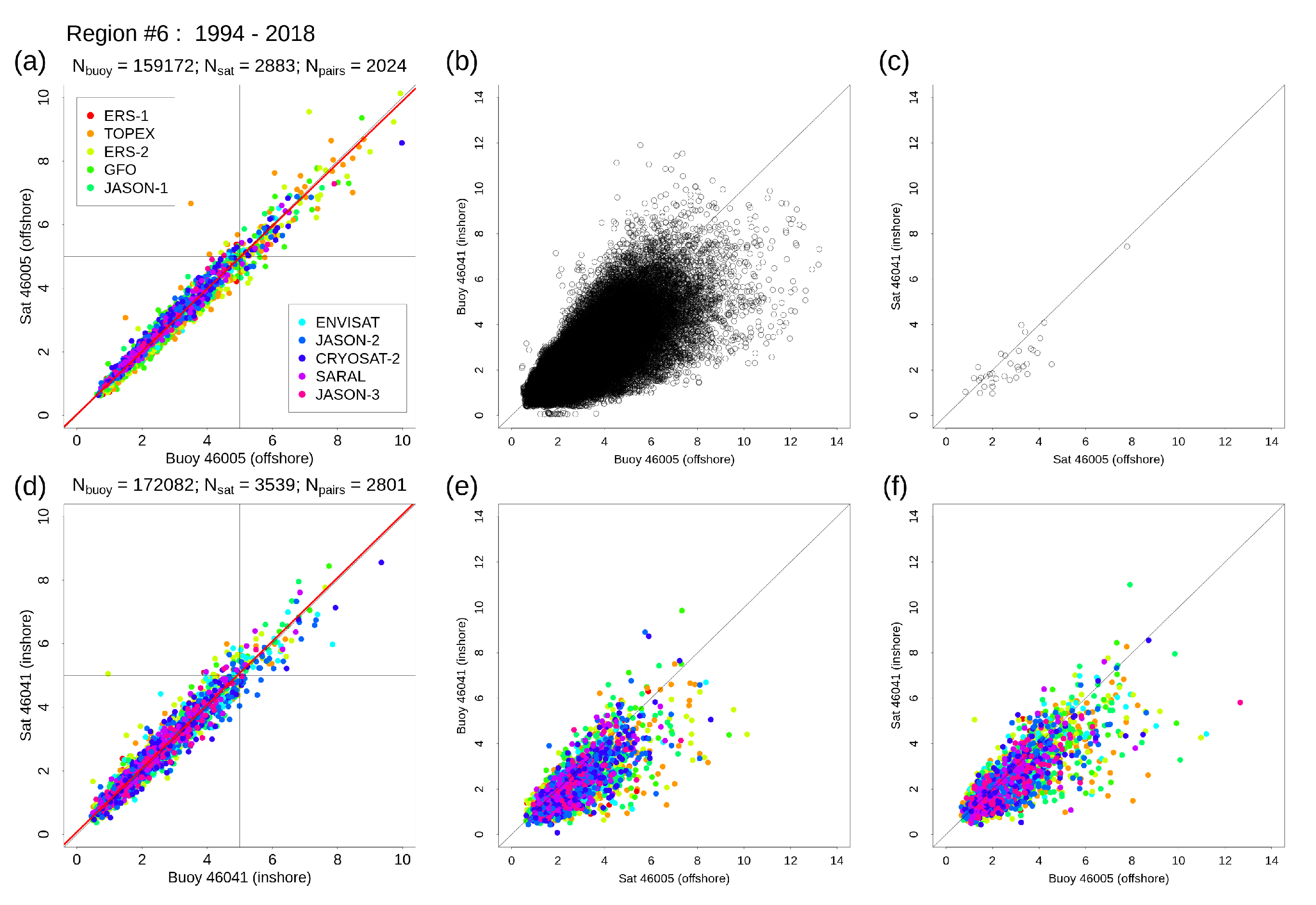
Interesting comparisons can be made with the other regions. Similar scatterplots for regions (#2 to #5) are provided in Figures S15–S18 in the supplementary information but we comment specifically on results from region #6 shown in Figure 9. The regression indicates excellent overall agreement but in terms of extremal agreement, the results are comparable with region #1. An absence of points in the top left and bottom right quadrants reveals that extremes are being captured accurately. For Hs above 6 m, differences are rarely greater than 1 m, and often less. At buoy 46005, the apparent lack of more recent missions capturing high energy events is likely related to mission orbital trajectories “missing” that particular location, and some loss of data from the buoy for extended periods of time in more recent years.

A more detailed explanation of the joint properties of the buoy pairs is beyond the scope of this analysis however we make a few observations regarding the difference between the east and west coast sites. Firstly, on the east coast and Gulf of Mexico there is a consistent pattern of high bias in the satellite measurements at the nearshore site, seen at regions #1, #2, #3 and #4. This pattern is not apparent in the two west coast regions (#5, #6). Due the limited number of comparisons these results cannot be said to be robust, nor is it clear that this applies to the most extreme observations. However, based on these findings we advocate for a more detailed investigation of this issue. Secondly, there is a clear difference in the joint characteristics between buoys. Figure 8b reveals a distinct absence of points in the upper left quadrant characterized by a strong alignment with the 1:1 line. However, on the west coast, seen in Figure 9b this feature is completely absent. This difference is likely due to the fetch limited conditions on the east coast created by prevailing offshore winds. In contrast, the west coast wave climate is predominantly dictated by easterly winds that cross the entire North Pacific basin. In this case, the same high waves impact both offshore and nearshore sites creating the somewhat “symmetric” looking joint structure seen in Figure 9b.

In respect of the extreme events jointly captured in all six regions, and whether offshore or nearshore, there are very few examples of large differences in Hs magnitudes. We have found little evidence to suggest that the extremes captured by satellites are deficient in any systematic way, although there does appear to be a limited dependency on geographic location. The exceptions to this are two east coast nearshore locations, at buoys 41110 and 41113 (Figures S14 and S15 respectively), where a strong positive bias in satellite measurements affects all the data, including the most extreme Hs values. It is particularly pronounced for buoy 41113. These two buoys are of the same “wave rider” design, lie in very shallow water (approximately 10 m and 20 m respectively) and have a fairly short duration of coverage (∼10 years). Without further detailed study it is difficult to speculate on the underlying causes of the systematic disagreement. In such shallow water, both depth-induced wave breaking and local currents are factors that may cause localised conditions that are not well captured by altimeters and re-tracking algorithms. It could also be that in such conditions the buoys also do not perform well and that the “true” value lies somewhere between the buoy and satellite measurements.

3.3. Impact of Under-Sampling on Extreme Analyses

Results suggest that the Sea State CCI L2P product generally gives a good representation of extreme Hs at distances of up to a few kilometers from the coast where it is limited primarily by low sampling of these events. The impact of this under-sampling on analysis depends upon many factors, including the wave climate at any given location. A detailed analysis for specific locations is beyond the scope of this paper but in order to quantify this impact in a general way, we have estimated Hs 10-year return level from the buoy data only, in regions #1, #4 and #5. These represent the east and west coast regions and the Gulf of Mexico, and provide the longest observational records (see Section 2.3 for methodological details). In order to approximate the effects of satellite under-sampling we have evaluated the 10-year return level based upon random sub-samples comprising only a percentage of the total data. 500 iterations of the sampling procedure were performed at each sub-sampling level in order to obtain average values of the return level and the 95% confidence bounds. This approach is intended to be approximately representative of the actual satellite sampling rates observed. For example, in Section 3.2 we showed that in region #1 (see Figure 8), the satellite data accounted for only 1.84% of the buoy time series for 1-h averages. This was almost the same (1.81%) in region #6 (see Figure 8). Although it is clear from Figure 6 that total annual data increases over time, for the purpose of convenience here only the average sampling rate it used. Note that similar analyses adopting variable annual rates gave similar results (not shown) and satellite estimates of 10-year return level were commensurate with results from sub-sampling at the appropriate level (typically <2%).

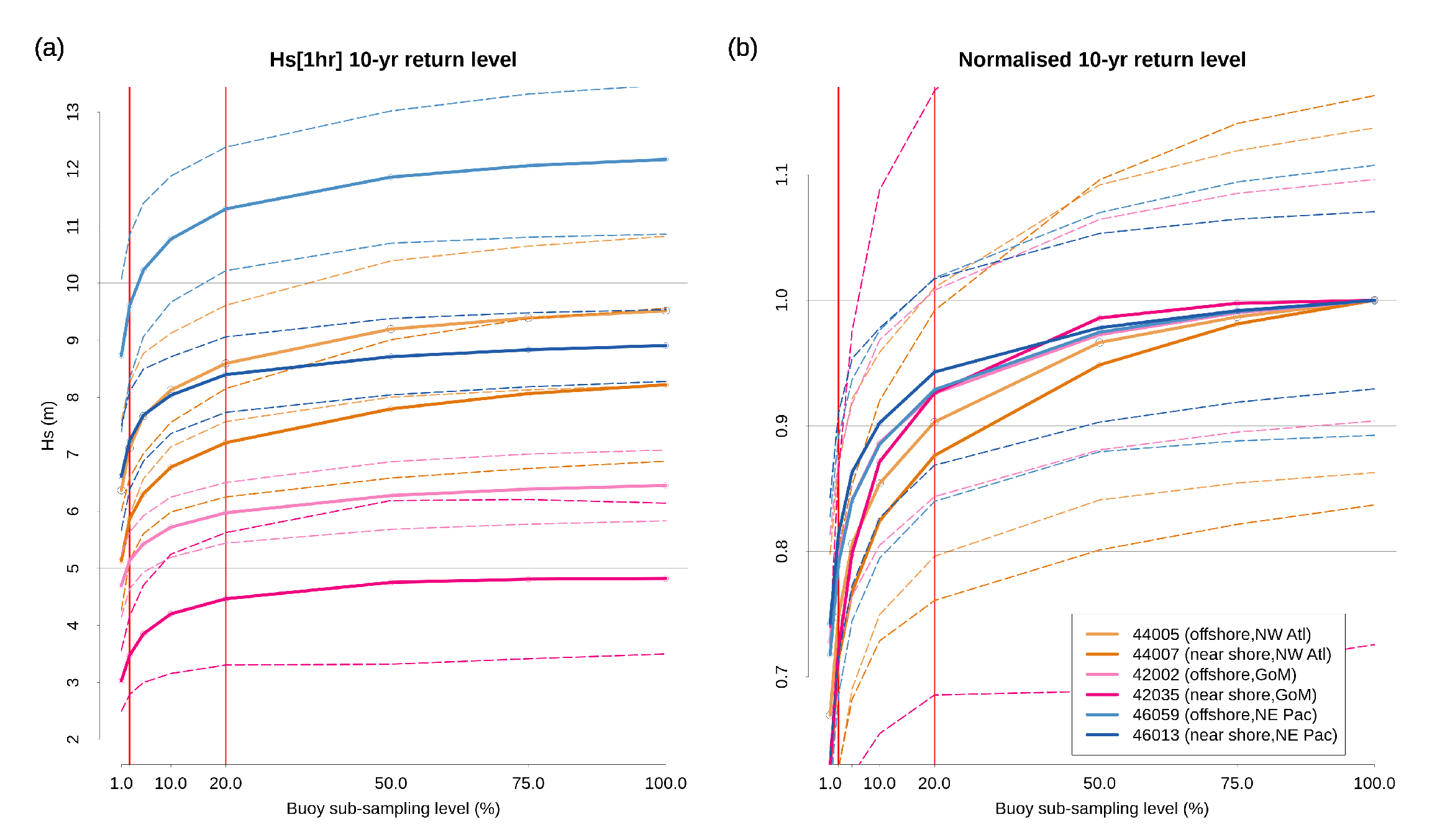
Figure 10 shows the Hs 10-year return level estimated at sampling levels between 1% and 100%. Figure 10a shows the estimates of absolute values of Hs, and it can be seen how these estimates are reduced as the level of sampling drops. Initially the decrease is fairly linear but below approximately 50% sampling the rate decreases nonlinearly and fairly substantial bias is introduced. Since this is a general approximation to the sampling rates seen in the Sea State CCI L2P product in any given geographic location, typically <2%, it is reasonable to expect that 10-year return level estimates would typically be severely underestimated. In Figure 10a,b, for reference, red vertical lines are marked at 2.5% and 20%. Figure 10b provides further insight. The curves (and uncertainty bounds) have been scaled by their 10-year return levels such that the common scale shows the difference in relative response to increased sampling. Some locations (such as NE Pacific) appear to be somewhat less affected by under-sampling than others (such as NW Atlantic). However, improvement in estimate due to increased sampling is not consistent across sites. Inspection of the uncertainty bounds reveals that once sampling is ∼20% of the total, the upper bound tends to exceed the “true” value. The red vertical line at 20% intersects a number of the upper bound (dashed) lines. An exception to this are the very wide confidence bounds for buoy 42035 in the Gulf of Mexico. While a detailed examination of this particular difference could be time consuming, we speculate that the impact of infrequent but powerful hurricanes is an important cause of this uncertainty. Infrequent high magnitude events, in a predominantly low magnitude climate, tend to substantially increase the uncertainty in fitting extreme value models due to very “long tails” in the probability distribution (see e.g., [27]). Regardless, these results suggest that under-estimation of 10-year return levels could be substantial where sampling remains below the 50% to 75% range.

4. Discussion

4.1. Data Quality and Geographic Variability

The Sea State CCI L2P product represents the state of the art in remotely observed sea state data. However, at the time of writing the project is ongoing, and revisions, including additional missions (e.g., Sentinel-3A) and refinements to calibration and re-tracking algorithms, are anticipated. It is perhaps no surprise therefore that in general we found excellent agreement with in situ measurements at most locations. Note also that, many of the wave buoys used in this study were also used for calibration of the Sea State CCI products, and therefore systematic differences in the overall long term record are expected to be small. However, primarily we have focused on the representation of extreme values at small scales close to the coast. The definition of “coastal scale” is not necessarily clear and in practice would depend on a specific application. Here, we have considered the range of approximately 10 to 100 km as representative, but also in part due to the requirement of co-locating with in situ data. Sites of specific interest could plausibly be on scales below 10 km. Regardless, it is clear from the results here and others [4] that even on larger scales, under-sampling is a substantial problem and so coastal applications on smaller scales will certainly face challenges in exploiting sea state data from satellite when investigating extreme conditions and their temporal variability.

What is promising however is that our results suggest in many geographic locations, observations of extremes very close to the coast, possibly even <5 km, are accurate. Use of the “good” data (qual_flag = 3) as flagged in the Sea State CCI L2P product, while sparse on small scales, is a valuable source of measurements where available. We also note that while not explicitly shown, measurements flagged as “poor” (qual_flag = 1) were indeed found to be spurious for the vast majority of cases and we do not advocate for their inclusion in analyses. Clearly, the geographic variability strongly manifests in all of our results. This stems, in a number of ways, from the highly heterogeneous nature of the sampling characteristics of the various satellite missions. As a result, a fixed sampling area such as the circle of 50 km radius employed here, will capture a remarkably variable number of mission tracks over any given period of time (see e.g., Figure 4). In addition, however, the local wave conditions and coastal morphology have a bearing on the effectiveness of the available data.

Although somewhat limited by the availability of long term in situ measurements, we have examined a range of locations which have highlighted some notable features. In particular, a consistent positive (negative) bias in the Sea State CCI data seen in the scatter plots for all nearshore (offshore) areas on the U.S. east coast. This is not apparent on the west coast. Furthermore, the positive bias nearshore at buoys 41110 and 41113 is substantial. So far we have not looked in more detail at either the prevailing wave conditions, or local coastal morphology. In such shallow water as at buoys 41110 and 41113, both depth limited breaking and even local ocean currents may be relevant. On the U.S. west coast, buoys lie at the end of the north Pacific storm track which typically drives long fetch wave systems. We do see good agreement between the Sea State CCI L2P and in situ data both nearshore and offshore (Figure 9 and Figure S18) and this may be linked to the regional wave climate. While satellite altimeter observations are not known to have strong, if any, error introduced by local wave climate characteristics, even in coastal regions (e.g., [19]), a more detailed investigation of this issue could consider directional or multivariate information.

4.2. Suitability of Satellite Observations for Analysis of Coastal Extremes and Variability

Studies of wave height extremes using satellite observations tend to be on a global scale [4,16,25,28] and these typically employ sampling areas of at least $2^{\circ }\times 2^{\circ }$ to mitigate the effects of low sampling rates. Even in these examples, correction methods are still required [4,28]. In the context of examining long term trends in extremes (up to 99th percentile), Jiang [4] goes to some lengths to examine ways of mitigating the errors induced by under-sampling. The “virtual observation” approach he describes is based upon the idea of using a secondary data source (reanalysis) to explain the missing data in the satellite record. Given these challenges at global scales, it is unsurprising that much less attention has been focused on using satellite wave height observations near the coast.

Where sampling levels based on 1-h averages drop as low as a few percent of in situ buoy data, it appears that smaller scale applications focused on investigating extreme variability will, for some time to come, continue to need to rely on diverse data sources and methods that can exploit and combine these together. However, the presence of albeit a limited amount of accurate data within a few kilometers of the coast motivates a number of possible avenues of development. For example, if local coastal wave conditions can be shown to be highly correlated over larger stretches of coastline, and further offshore, then simple areal aggregation can immediately and substantially increase the quantity of available data. Indeed, others have already proposed methods to combine in situ and modeled wave data to generate improved estimates of Hs extremes and return times [29]. Jiang [30] describes an approach to validation based upon exploiting spatial structures found in simulated datasets to combat the issue of sparse sampling. Furthermore, an awareness of the particular missions and tracks that contribute to the data at a specific location can guide the choice of sample aggregation area in order to maximise available and relevant observations. From there, variations of methods such as the “virtual observation” approach described by [4] could be applied to local coastal scale reanalysis or hindcast datasets in order to develop appropriate corrections.

Beyond this, further extensions of such methods might involve more explicit spatial statistical modeling of extremes. The extreme value modeling approaches described by [25,28,31] rely on analysing observations partitioned into individual grid cells but importantly do not take advantage of spatially correlated information. Methods similar to those described by [17,32] involve extreme value models that exploit the spatial dependence structure of the data, and also account for temporal variability, allowing for investigation of long term trends. Such approaches reduce uncertainty in estimates of long period return levels. Even more sophisticated methods can capture the spatial dependence structure in the extremes and have already been applied to ocean wave data in certain contexts [5]. While appealing, it is not clear that any of these methods alone can be applied to satellite data “as is” but some hybrid of the methods cited here appears to be a promising line of investigation that could lead to a more generally applicable and productive approach to the analysis of coastal extremes and their variability from satellite observations.

5. Conclusions

We have conducted a detailed study of the sampling characteristics of satellite data provide in the ESA Sea State CCI L2P v1.1 product at a number of locations in a range of geographic regions around the U.S. coasts. These observational data were compared with in situ data and found to agree very well in the extremes, even close to the coast (up to 5 km), but suffered from low levels of spatio-temporal sampling that typically drop dramatically within a few kilometres of the coast. Low sampling led to large underestimates of 10-year Hs return levels determined from a basic extreme value method. In spite of the potential to mitigate the absence of in situ measurements in most of the worlds coastal regions, we judge that analyses of extreme variability on coastal scales using the Sea State CCI dataset alone remains challenging. However, although sparse on small spatial scales, measurements of extremes tend to be accurate, and we suggest they may be exploited effectively through careful inspection and the application of hybrid methods that have so far been described in the literature in various settings.

References

1. Ribal, A.; Young, I.R. 33 years of globally calibrated wave height and wind speed data based on altimeter observations. Sci. Data 2019, 6, 1–15. [Google Scholar] [CrossRef] [Green Version]
2. Morim, J.; Hemer, M.; Wang, X.L.; Cartwright, N.; Trenham, C.; Semedo, A.; Young, I.; Bricheno, L.; Camus, P.; Casas-Prat, M.; et al. Robustness and uncertainties in global multivariate wind-wave climate projections. Nat. Clim. Chang. 2019, 9, 711–718. [Google Scholar] [CrossRef] [Green Version]
3. Timmermans, B.; Gommenginger, C.; Dodet, G.; Bidlot, J.R. Global Wave Height Trends and Variability from New Multimission Satellite Altimeter Products, Reanalyses, and Wave Buoys. Geophys. Res. Lett. 2020, 47, 1–11. [Google Scholar] [CrossRef]
4. Jiang, H. Evaluation of altimeter undersampling in estimating global wind and wave climate using virtual observation. Remote Sens. 2020, 245, 111840. [Google Scholar] [CrossRef]
5. Shooter, R.; Tawn, J.; Ross, E.; Jonathan, P. Basin-wide spatial conditional extremes for severe ocean storms. Extremes 2020. [Google Scholar] [CrossRef]
6. Dodet, G.; Piolle, J.F.; Quilfen, Y.; Abdalla, S.; Accensi, M.; Ardhuin, F.; Ash, E.; Bidlot, J.R.; Gommenginger, C.; Marechal, G.; et al. The Sea State CCI dataset v1: Towards a Sea State Climate Data Record based on satellite observations. Earth Syst. Sci. Data 2020. [Google Scholar] [CrossRef]
7. Piollé, J.F.; Dodet, G.; Quilfen, Y. ESA Sea State Climate Change Initiative: Global Remote Sensing Multi-Mission Along-Track Significant Wave Height, L2P Product, Version 1.1., Centre for Environmental Data Analysis; Technical Report; European Space Agency, CCI for Sea State Consortium: Plymouth, UK, 2020. [CrossRef]
8. Piollé, J.F.; Dodet, G.; Quilfen, Y. ESA Sea State Climate Change Initiative: Global Remote Sensing Merged Multi-Mission Monthly Gridded Significant Wave Height, L4 Product, Version 1.1, Centre for Environmental Data Analysis; Technical Report; European Space Agency, CCI for Sea State Consortium: Plymouth, UK, 2020. [CrossRef]
9. Cardone, V.J.; Callahan, B.T.; Chen, H.; Cox, A.T.; Morrone, M.A.; Swail, V.R. Global distribution and risk to shipping of very extreme sea states (VESS). Int. J. Climatol. 2015, 35, 69–84. [Google Scholar] [CrossRef]
10. Storlazzi, C.D.; Gingerich, S.B.; van Dongeren, A.; Cheriton, O.M.; Swarzenski, P.W.; Quataert, E.; Voss, C.I.; Field, D.W.; Annamalai, H.; Piniak, G.A.; et al. Most atolls will be uninhabitable by the mid-21st century because of sea-level rise exacerbating wave-driven flooding. Sci. Adv. 2018, 4. [Google Scholar] [CrossRef] [PubMed] [Green Version]
11. Patlakas, P.; Stathopoulos, C.; Tsalis, C.; Kallos, G. Wind and wave extremes associated with tropical-like cyclones in the Mediterranean basin. Int. J. Climatol. 2019, 1–22. [Google Scholar] [CrossRef]
12. Hemer, M.A. Historical trends in Southern Ocean storminess: Long-term variability of extreme wave heights at Cape Sorell, Tasmania. Geophys. Res. Lett. 2010, 37, 1–5. [Google Scholar] [CrossRef]
13. Bender, L.C., III; Guinasso, N.L., Jr.; Walpert, J.N.; Howden, S.D. A Comparison of Methods for Determining Significant Wave Heights—Applied to a 3-m Discus Buoy during Hurricane Katrina. J. Atmos. Ocean. Technol. 2010, 27, 1012–1028. [Google Scholar] [CrossRef]
14. Gemmrich, J.; Thomas, B.; Bouchard, R. Observational changes and trends in northeast Pacific wave records. Geophys. Res. Lett. 2011, 38. [Google Scholar] [CrossRef]
15. Meucci, A.; Young, I.R.; Aarnes, O.J.; Øyvind, B. Comparison of Wind Speed and Wave Height Trends from Twentieth-Century Models and Satellite Altimeters. J. Clim. 2020, 33, 611–624. [Google Scholar] [CrossRef]
16. Young, I.R.; Ribal, A. Multiplatform evaluation of global trends in wind speed and wave height. Science 2019, 364, 548–552. [Google Scholar] [CrossRef]
17. Calafat, F.M.; Marcos, M. Probabilistic reanalysis of storm surge extremes in Europe. Proc. Natl. Acad. Sci. USA 2020, 117, 1877–1883. [Google Scholar] [CrossRef] [Green Version]
18. Hiles, C.E.; Robertson, B.; Buckham, B.J. Extreme wave statistical methods and implications for coastal analyses. Estuar. Coast. Shelf Sci. 2019, 223, 50–60. [Google Scholar] [CrossRef]
19. Wiese, A.; Staneva, J.; Schulz-Stellenfleth, J.; Behrens, A.; Fenoglio-Marc, L.; Bidlot, J.R. Synergy of wind wave model simulations and satellite observations during extreme events. Ocean Sci. 2018, 16, 1503–1521. [Google Scholar] [CrossRef] [Green Version]
20. Nencioli, F.; Quartly, G.D. Evaluation of Sentinel-3A Wave Height Observations Near the Coast of Southwest England. Remote Sens. 2019, 11, 2998. [Google Scholar] [CrossRef] [Green Version]
21. Schlembach, F.; Passaro, M.; Quartly, G.D.; Kurekin, A.; Nencioli, F.; Dodet, G.; Piollé, J.F.; Ardhuin, F.; Bidlot, J.; Schwatke, C.; et al. Round Robin Assessment of Radar Altimeter Low Resolution Mode and Delay-Doppler Retracking Algorithms for Significant Wave Height. Remote Sens. 2020, 12, 1254. [Google Scholar] [CrossRef] [Green Version]
22. Quartly, G.D.; Kurekin, A.A. Sensitivity of Altimeter Wave Height Assessment to Data Selection. Remote Sens. 2020, 12, 2608. [Google Scholar] [CrossRef]
23. Piollé, J.F.; Dodet, G.; Ash, E. ESA Sea State Climate Change Initiative: Product User Guide, Version 1.0; Technical Report; European Space Agency, CCI for Sea Sate Consortium: Plymouth, UK, 2020.
24. Coles, S. An Introduction to Statistical Modeling of Extreme Values; Springer: London, UK, 2001. [Google Scholar]
25. Izaguirre, C.; Méndez, F.J.; Menéndez, M.; Losada, I.J. Global extreme wave height variability based on satellite data. Geophys. Res. Lett. 2011, 38, 1–6. [Google Scholar] [CrossRef]
26. Wessel, P.; Smith, W.F. A global, self-consistent, hierarchical, high-resolution shoreline database. J. Geophys. Res. Solid Earth 1996, 101, 8741–8743. [Google Scholar] [CrossRef] [Green Version]
27. Timmermans, B.; Stone, D.; Wehner, M.; Krishnan, H. Impact of tropical cyclones on modeled extreme wind-wave climate. Geophys. Res. Lett. 2017, 44, 1393–1401. [Google Scholar] [CrossRef]
28. Takbash, A.; Young, I.R.; Øyvind, B. Global Wind Speed and Wave Height Extremes Derived from Long-Duration Satellite Records. J. Clim. 2019, 32, 109–126. [Google Scholar] [CrossRef]
29. Dentale, F.; Furcolo, P.; Carratelli, E.P.; Reale, F.; Contestabile, P.; Tomasicchio, G.R. Extreme Wave Analysis by Integrating Model and Wave Buoy Data. Water 2018, 10, 373. [Google Scholar] [CrossRef] [Green Version]
30. Jiang, H. Indirect Validation of Ocean Remote Sensing Data via Numerical Model: An Example of Wave Heights from Altimeter. Remote Sens. 2020, 12, 2627. [Google Scholar] [CrossRef]
31. Kumar, P.; Min, S.K.; Weller, E.; Lee, H.; Wang, X.L. Influence of Climate Variability on Extreme Ocean Surface Wave Heights Assessed from ERA-Interim and ERA-20C. J. Clim. 2016, 29, 4031–4046. [Google Scholar] [CrossRef]
32. Risser, M.D.; Paciorek, C.J.; Wehner, M.F.; O’Brien, T.A.; Collins, W.D. A probabilistic gridded product for daily precipitation extremes over the United States. Clim. Dyn. 2019, 53, 2517–2538. [Google Scholar] [CrossRef] [Green Version]
Figure 1. Map of the six regions indicated by blue boxes, and the associated NDBC moored data buoys.
Jmse 08 01039 g001
Figure 2. Total number of observations per 1 km bin, and proportion of data associated with good quality and rejection flags, as a function of distance to the coast, for region #1 on the north east U.S. coast. The (a) first 10 years and (b) last 10 years of the Sea State CCI L2P satellite record are shown.
Jmse 08 01039 g002
Figure 3. Total number of observations per 1 km bin, and proportion of data associated with good quality and rejection flags, as a function of distance to the coast, for region #2 on the east U.S. coast. The (a) first 10 years and (b) last 10 years of the Sea State CCI L2P satellite record are shown.
Jmse 08 01039 g003
Figure 4. Spatial distribution of satellite tracks contributing to Hs measurements within a 50 km radius of buoy 41113 (region #3).
Jmse 08 01039 g004
Figure 5. Total number of good (qual_flag = 3) Hs observations per year in region #1, (a) at nearshore buoy 44007 and (b) offshore buoy 44005 based upon a 50 km sampling radius around each buoy.
Jmse 08 01039 g005
Figure 6. Total number of good (qual_flag = 3) Hs observations per year in region #2, (a) at nearshore buoy 41110 and (b) offshore buoy 41002 based upon a 50 km sampling radius around each buoy.
Jmse 08 01039 g006
Figure 7. A comparison of measurements of Hs from buoy 41010 and satellite, based upon a 50 km sampling radius. Data with all quality flags (qual_flag = [1,2,3]) is shown in (a,b). (a) shows the time series from the buoy overlaid by the complete 1 Hz record from the Sea State CCI L2P product. Selected rejection flags are indicated by blue diamonds with values on the right-hand axis. Blue horizontal lines correspond to the right-hand axis and denote the rejection values more clearly. (b) is an enlargement of a section of (a) indicated by vertical black lines, and shows the same data but coloured by mission. (c) is similar to (b) but shows the median value (black crosses) of each track segment for 1 Hz measurements where qual_flag = 3 applied.
Jmse 08 01039 g007
Figure 8. Scatter plots showing pairwise 1-h observations in region #1, at 44005 (offshore) and 44007 (nearshore) for combinations of source data and locations. (a,d) show Sea State CCI L2P vs. buoys 44005 and 44007 respectively. Red lines (a,b) show the fit of linear major-axis regression models to the entire data set. (b,c,e,f) show comparisons of the remaining combinations of source data and location. Colouring by mission is applied to selected panels where this makes sense.
Jmse 08 01039 g008
Figure 9. Scatter plots for pairwise 1-h observations in region #6, at 46005 (offshore) and 46041 (nearshore) for combinations of source data and locations. (a,d) show Sea State CCI L2P vs. buoys 46005 and 46041 respectively. Red lines (a,b) show the fit of linear major-axis regression models to the entire data set. (b,c,e,f) show comparisons of the remaining combinations of source data and location. Colouring by mission is applied to selected panels where this makes sense.
Jmse 08 01039 g009
Figure 10. 10-year return levels computed from 1-h averaged buoy measurements of Hs as a function of percentage of total possible sampling at a number of nearshore and offshore buoys. Solid lines show the point estimate (based on an iterative average) and dashed lines show the upper and lower 95% confidence bounds. Red vertical lines indicate the 2.5% and 20% sampling levels. (a) shows absolute value of return level. (b) shows the same values but normalised to the value obtained from the totality of the data.
Jmse 08 01039 g010
Publisher’s Note: MDPI stays neutral with regard to jurisdictional claims in published maps and institutional affiliations.