Accuracy of the Cell-Set Model on a Single Vane-Type Vortex Generator in Negligible Streamwise Pressure Gradient Flow with RANS and LES

Abstract

Passive flow control devices are included in the design of wind turbine blades in order to obtain better performance and reduce loads without consuming any external energy. Vortex Generators are one of the most popular flow control devices, whose main objective is to delay the flow separation and increase the maximum lift coefficient. Computational Fluid Dynamics (CFD) simulations of a Vortex Generator (VG) on a flat plate in negligible streamwise pressure gradient conditions with the fully-resolved mesh model and the cell-set model using Large Eddy Simulation (LES) and Reynolds-Averaged Navier-Stokes (RANS) were carried out, with the objective of evaluating the accuracy of the cell-set model taking the fully-resolved mesh model as benchmark. The implementation of the cell-set model entailed a considerable reduction of the number of cells, which entailed saving simulation time and resources. The coherent structures, vortex path, wall shear stress and size, strength and velocity profiles of the primary vortex have been analyzed. The results show good agreements between the fully-resolved mesh model and the cell-set mode with RANS in all the analyzed parameters. With LES, acceptable results were obtained in terms of coherent structures, vortex path and wall shear stress, but slight differences between models are visible in the size, strength and velocity profiles of the primary vortex. As this is considered the first application of the cell-set model on VGs, further research is proposed, since the implementation of the cell-set model can represent an advantage over the fully-resolved mesh model.

1. Introduction

Wind energy has become a key source of electricity generation for the change to a cleaner and sustainable energy model. In order to compete in energy production and cost against the traditional energies, improvement and optimization of wind turbines is required.

To improve the efficiency of wind turbine blades, both active (such as trailing edge flaps, air jet vortex generators and synthetic jets) and passive devices (such as vortex generators, microtabs, spoilers, fences, serrated trailing edge and Gurney flaps) can be added. Aramendia et al. [1] and Aramendia-Iradi et al. [2] thoroughly reviewed both active and passive flow control devices. Among these two types of devices, passive devices can be highlighted, since they improve performance of wind turbine blades without consuming any external energy.

Vortex Generators (VGs) are one of the most popular passive flow control devices due to their simplicity, effectiveness and low cost for both production and installation. They are small vanes which are located at the extrados of a lifting surface with an angle of inclination with the inflow. They are usually triangular or rectangular, and are frequently displayed in pairs. The main target of these devices is to delay the flow separation and increase the maximum lift coefficient, transferring the energy produced in the outer region to the boundary layer region.

Since their introduction by Taylor [3], VGs have been a research topic due to their wide range of applications in aerodynamics. Several experimental studies have been carried out over the years to analyze the influence of VGs on flow, such as Awais and Bhuiyan [4]. However, nowadays, with the increase in computer calculation speed, numerical studies using Computational Fluid Dynamics (CFD) are becoming the most effective choice for the analysis and optimization of VGs.

Urkiola et al. [5] and Fernandez-Gamiz et al. [6] performed CFD simulations to study the vortices generated by a passive rectangular vane-type VG on a flat plate with a negligible pressure gradient flow, and compared the obtained results with experimental data. In both studies, good agreements between the numerical and experimental results were obtained, but Urkiola et al. [5] found some discrepancies in the predictions of the primary vortex generated by the VG, especially at high incident angles. They attributed these discrepancies to the selected turbulence model. Following these studies, Ibarra-Udaeta et al. [7] and Martínez-Filgueira et al. [8] analyzed the same case with different vane heights and incident angles. All of them used the fully-resolved mesh model.

Despite the simple geometry of the VGs, the fully-resolved mesh model requires a very fine mesh in the area near the VG, which, combined with the large computational domain, makes the number of cells unnecessarily high. For this reason, numerous authors have implemented alternative models to study VGs, in order to reduce the computational and mesh design time that the simulations performed with the fully-resolved mesh model require.

The jBAY source term model presented by Jirasek [9] based on the Bender-Anderson-Yagle (BAY) model developed by Bender et al. [10] is one of the most popular alternative models. This model substitutes the VG geometry by a subdomain of similar size at the location of the original VG. Despite not being a meshed geometry, this model applies a force perpendicular to the local flow direction. Many authors have implemented this model in their studies because of the significant reduction of the number of cells that its application entails. For instance, Ballesteros-Coll et al. [11] and Chillon et al. [12] implemented triangular VGs based on the jBAY source term model on the DU97W300 airfoil. Errasti et al. [13] analyzed the accuracy of the jBAY source term model in conventional and in sub-boundary layer vane-type VGs under an adverse pressure gradient, showing fairly accurate results for the jBAY source term model, especially in the conventional VG.

Fernandez-Gamiz et al. [14] compared four different models of VGs, including a fully-resolved mesh VG model, an Actuator VG Model (AcVG) based on the BAY model developed by Bender [10] and an experimental VG model. Despite obtaining similar results in terms of vortex development, their study shows significant differences between the numerical and experimental results.

Another alternative model is the cell-set model. This model is similar to the jBAY source-term model, but in this case, the geometry is created by leveraging the mesh, so the geometry is meshed and the force it makes on the flow does not have to be modelled. Despite the resource savings involved in applying this model, there are very few studies in which it has been used. For example, in the previously-mentioned study of Ballesteros-Coll et al. [11] a Gurney flap was generated with this model, but the present study is the first time where it has been applied to VGs, at least to the knowledge of the authors.

In the majority of the above-mentioned CFD studies, Reynolds-Averaged Navier-Stokes (RANS) based turbulence models are selected. Although the results in most cases are good, as mentioned above, there are cases where RANS turbulence models do not provide the desired accuracy. In those cases, despite the high computational cost, Large Eddy Simulation (LES) turbulence models are a good choice. This has led to many authors using LES turbulence models for the analysis of wind turbines and their devices. Solís-Gallego et al. [15] analyzed the FX 63-137 airfoil using LES, Bjerg et al. [16] analyzed the flow structures of 25 different configurations of VG pairs by LES, and Saha et al. [17] investigated the coherent structures of a vane-type rectangular VG pair with a high incident angle.

Colleoni et al. [18] developed an innovative design of a solar plate receiver with VGs, and carried out CFD simulations using both RANS and LES turbulence models. The results show that LES allows for a better understanding of the behavior of the generated vortices and thermal exchanges.

This paper aims to analyze the capability of the cell-set model to reproduce the physics of the wake downstream of a VG on a flat plate in a negligible streamwise pressure gradient flow. As the above-mentioned studies demonstrate, the fully-resolved mesh model provides accurate results in VG problems. Therefore, CFD simulations are carried out using the fully-resolved mesh model and the cell-set model, and the obtained results are compared, in order to evaluate the accuracy of the cell-set model taking the fully-resolved mesh model as benchmark. RANS and LES turbulence models are selected in order to study the accuracy of the cell-set model with both turbulence models.

2. Numerical Setup

Numerical simulations were carried out in order to analyze the accuracy of cell-set model in a VG on a flat plate in a negligible streamwise pressure gradient flow. To conduct the simulations, Star CCM+v14.02.012 [19] CFD commercial code was used.

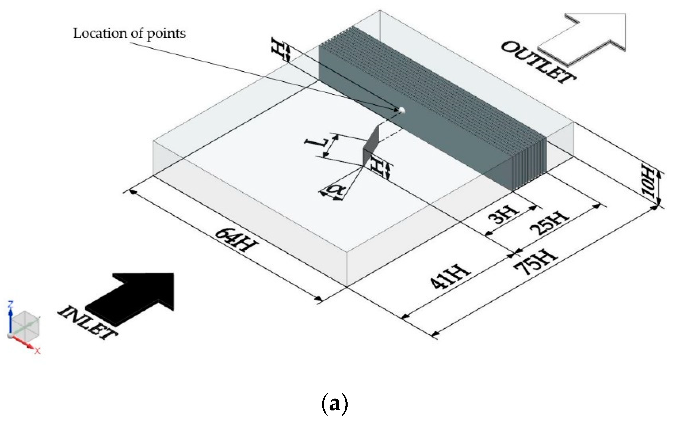
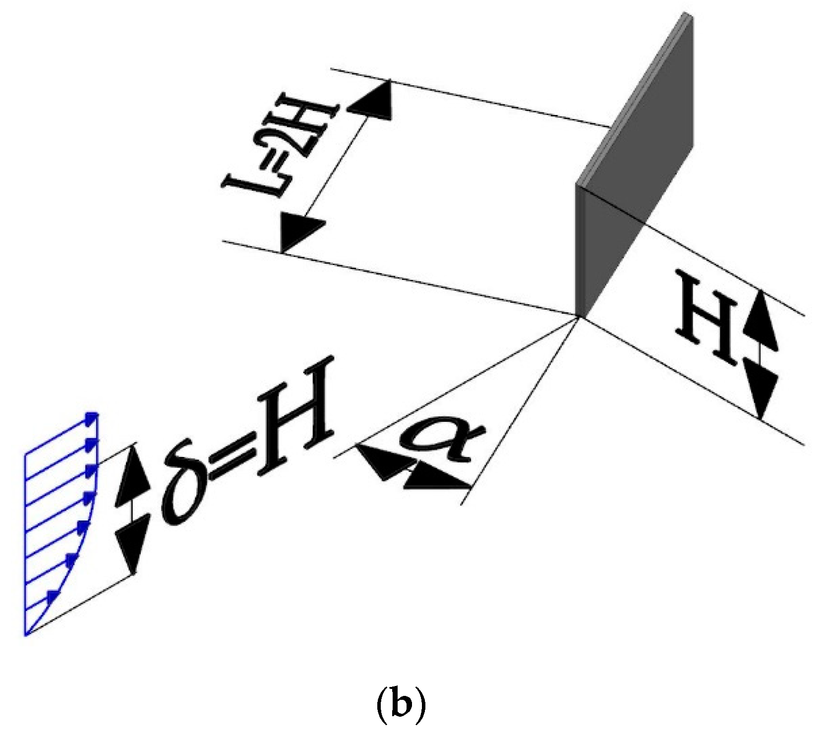
2.1. Computational Domain

The computational domain consists of a block with a rectangular VG located on its lower surface. The height of the VG (H) is equal to 0.25 m and the length (L) is twice its height. Two different incident angles (α) are considered, 18° and 25°. The lower surface of the block and the surfaces of the VG are considered walls with no-slip conditions, the upstream part of the domain is set as inlet and the downstream part of the domain is set as outlet. The rest of the surfaces are considered symmetry planes, in order not to affect the flow. The computational domain and the distance from the inlet to the VG position were designed in order to have the boundary layer thickness (δ) at the VG position equal to the height of the VG (δ = H). More information about the computational domain is shown in Figure 1.

For data extraction 12 points and 12 spanwise planes normal to the streamwise direction are considered. The planes are located from 3H to 25H of the LE (Leading Edge), separated 2H between each other. The points are located on the planes, downstream the TE (Trailing Edge) of the VG, at a height of 1H from the wall.

2.2. Physics Models

A three-dimensional incompressible flow with constant values of 1.225 ${\mathrm{kg}/\mathrm{m}}^3$ for density (ρ) and $1{.85185\text{ × }10}^{-4}{\mathrm{m}}^2/\mathrm{s}$ for kinematic viscosity ($v$) is considered. The free stream velocity ($U_{\infty }$) of the flow is set at 20 m/s, which means that the Reynolds number (Re) is around 27,000 according to Equation (1).

$$Re=\frac{U_{\infty }·\delta }{v}$$

(1)

Two different turbulence models were selected for the simulations, Menter’s k-ω SST (Shear Stress Transport) [20] RANS-based turbulence model for the simulations in which the incident angle is equal to 18° and LES Smagorinsky SGS (sub-grid-scale) [21] model for the simulations in which the incident angle is equal to 25°. Allan et al. [22] analyzed the flow field of a single VG on a flat plate with two different angles of attack, and showed that RANS-based simulations agree well with the experimental data, except for short distances downstream of the vane. In their study, a better performance of the SST turbulence model was found in comparison with other RANS turbulence models. RANS and LES turbulence models were selected for two main reasons. The first reason is that performing simulations with these two turbulence models allows one to analyze the accuracy of the cell-set model in both RANS and LES. The second reason is that, as shown by Urkiola et al. [5], when working with high incident angles, RANS is not able to accurately capture flow characteristics; therefore, LES is more appropriate when α = 25°.

For RANS-based simulations, a full second order linear-upwind scheme for the domain discretization has been used [23]. In LES, the large scales of the turbulence are directly resolved everywhere in the flow domain, and the small-scale motions are modelled. In contrast to the RANS equations, the equations that are solved for LES are obtained by a spatial filtering rather than an averaging process. Therefore, the variables of the flow are divided into a filtered value and a sub-grid value. The filtered values are inserted in the Navier-Stokes equations. To give closure to these equations, the SGS stress tensor is modelled by an SGS model.

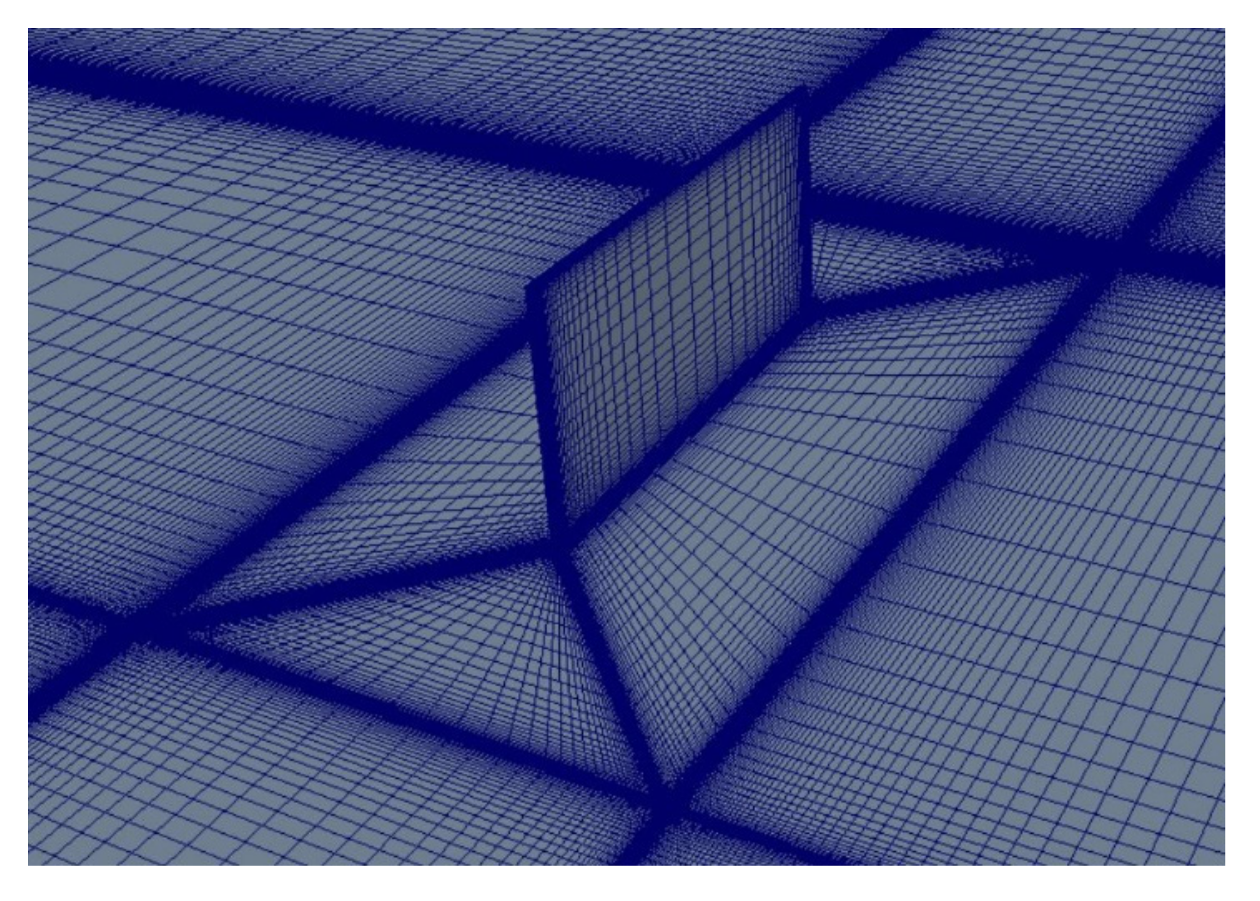
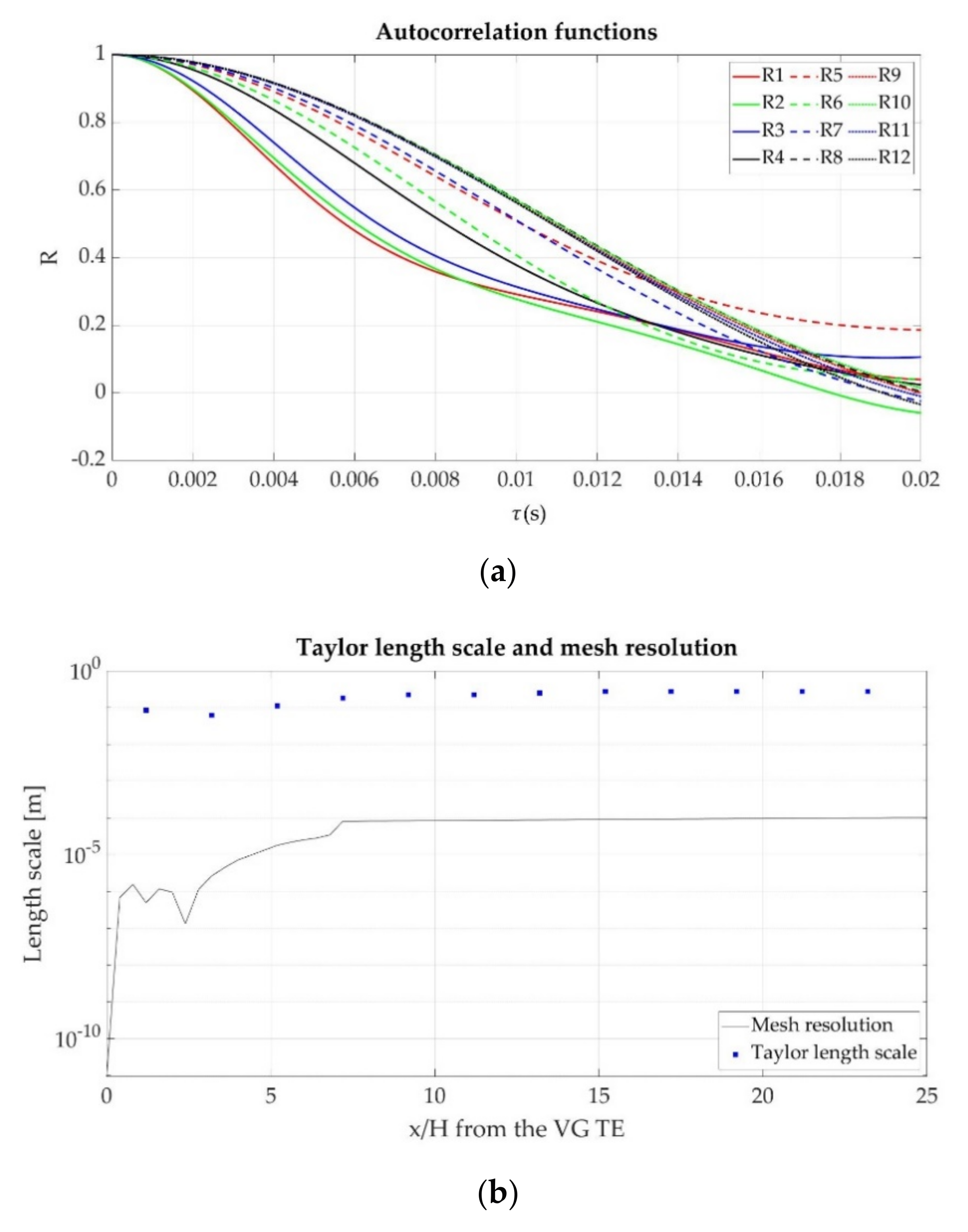
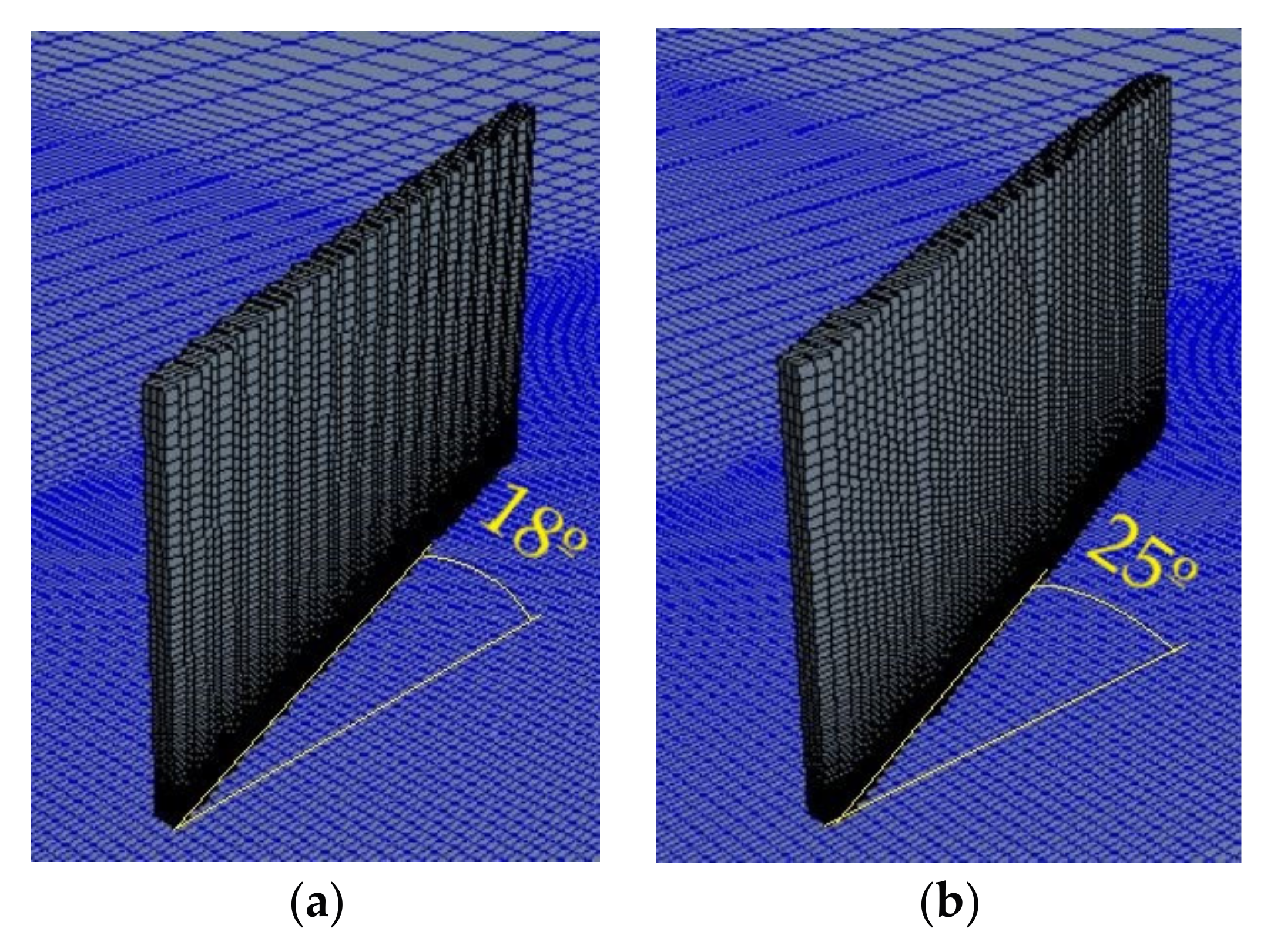
2.3. Fully-Resolved Mesh Model

A structured mesh of around 11.5 million hexahedral cells was generated. In order to enhance the accuracy of the results in the area near the VG, the cell density is much higher in this region. Figure 2 shows the refined mesh near the VG. This mesh was used for both cases (α = 18° and α = 25°), rotating it depending on the desired incident angle.

The General Richardson Extrapolation method [24] applied to lift and drag forces of the VG was performed in order to verify sufficient mesh resolution for RANS. This method estimates the value of the analyzed parameter when the cell quantity tends to infinite. For more information about the General Richardson Extrapolation method, check Almohammadi et al. [25]. According to Stern et al. [26], a convergence study requires a minimum of three mesh solutions. Apart from the above-mentioned mesh (which is considered the fine mesh), a medium mesh and a coarse mesh were generated. Furthermore, as recommended, geometrically similar grids were used along with structured grid refinement. The results show that the convergence condition (R) is between 0 and 1, which means that the tendency is a monotonic convergence. In addition, the estimated values (RE) of lift and drag forces are close to the values obtained from the simulations with the fine mesh. Thus, the mesh resolution is adequate for RANS.

Table 1. Mesh verification for Reynolds-Averaged Navier-Stokes (RANS).

Variable	Mesh Resolution			Richardson Extrapolation
	Coarse [N]	Medium [N]	Fine [N]	RE [N]	p	R
Drag force	98.0699	89.8929	87.199	85.875	1.6018	0.329
Lift force	261.605	247.715	241.39	236.1	1.135	0.455

shows the results of the General Richardson Extrapolation.

Verification of sufficient mesh resolution for LES was performed based on the criterion stablished by Kuczaj et al. [27]. According to their study, the mesh resolution ($\Delta =\sqrt[3]{V_{cell}}$) should at least be in order of the Taylor length-scale (λ) to completely solve the Taylor length-scale. Taylor length-scale is obtained from the Taylor expansion coefficient of the autocorrelation function about the origin. The autocorrelation function defines the relation between data samples in a time series, on average, to the preceding data points. This function is useful to analyze how turbulent a flow is. The more turbulent the flow, the lower the relationship between the data. Consequently, the auto-correlation function will approach zero faster. From the autocorrelation function, the Taylor time-scale is calculated, and finally, the Taylor length-scale is estimated by the Taylor hypothesis [28]. For more information about the Taylor length-scale calculation process, check [27,29]. This method has been applied in the previously-mentioned 12 points. The autocorrelation functions of different points are shown in Figure 3a and the comparison between the Taylor length-scale and mesh resolution is plotted in Figure 3b.

The results show that autocorrelation functions tend progressively to 0. This is due to the negligible streamwise pressure gradient conditions that have been assigned to the flow. This has resulted in a significant difference between Taylor length-scale and mesh resolution, which fulfills the criteria proposed by Kuczaj et al. [27]. Hence, the mesh is suitable for LES simulations.

2.4. Cell-Set Model

In the present work, the accuracy of the cell-set model applied on VGs is studied. To implement this model, a mesh without VG is generated, then the required geometry (in this case the VG) is defined. To define the VG, the mesh is leveraged by using the cells where the VG should be located. Once the geometry is defined, the cells which are around the geometry are selected, a new cell-set region is created with those cells and a wall boundary is assigned to that region. For more information about the cell-set model implementation process, check Ballesteros-Coll et al. [11]. Figure 4 shows the cell-set construction of the VG with the cell-set model.

In comparison with the fully-resolved mesh, a coarser mesh can be designed when using the cell-set model, saving computational time and resources. In this case, the meshes generated with this model consist of around 7.2 million cells.

3. Results and Discussions

In this paper, the vortexes generated by a vane-type VG on a flat plate are analyzed with the objective of comparing the results obtained with the fully-resolved mesh model and the cell-set model. With that aim, the primary vortex path, size, strength and velocity profiles have been analyzed. In addition, the coherent structures and wall shear stress have been studied.

For all the simulations, parallel computing with 56 Intel Xeon 5420 cores and 45 GB of RAM were used. Simulations in which the fully-resolved mesh model was used were run for 170,334 s using the RANS turbulence model and 663,595 s using the LES model. In contrast, simulations in which the cell-set model was used were run for 103,120 s for RANS and 401,070 s for LES.

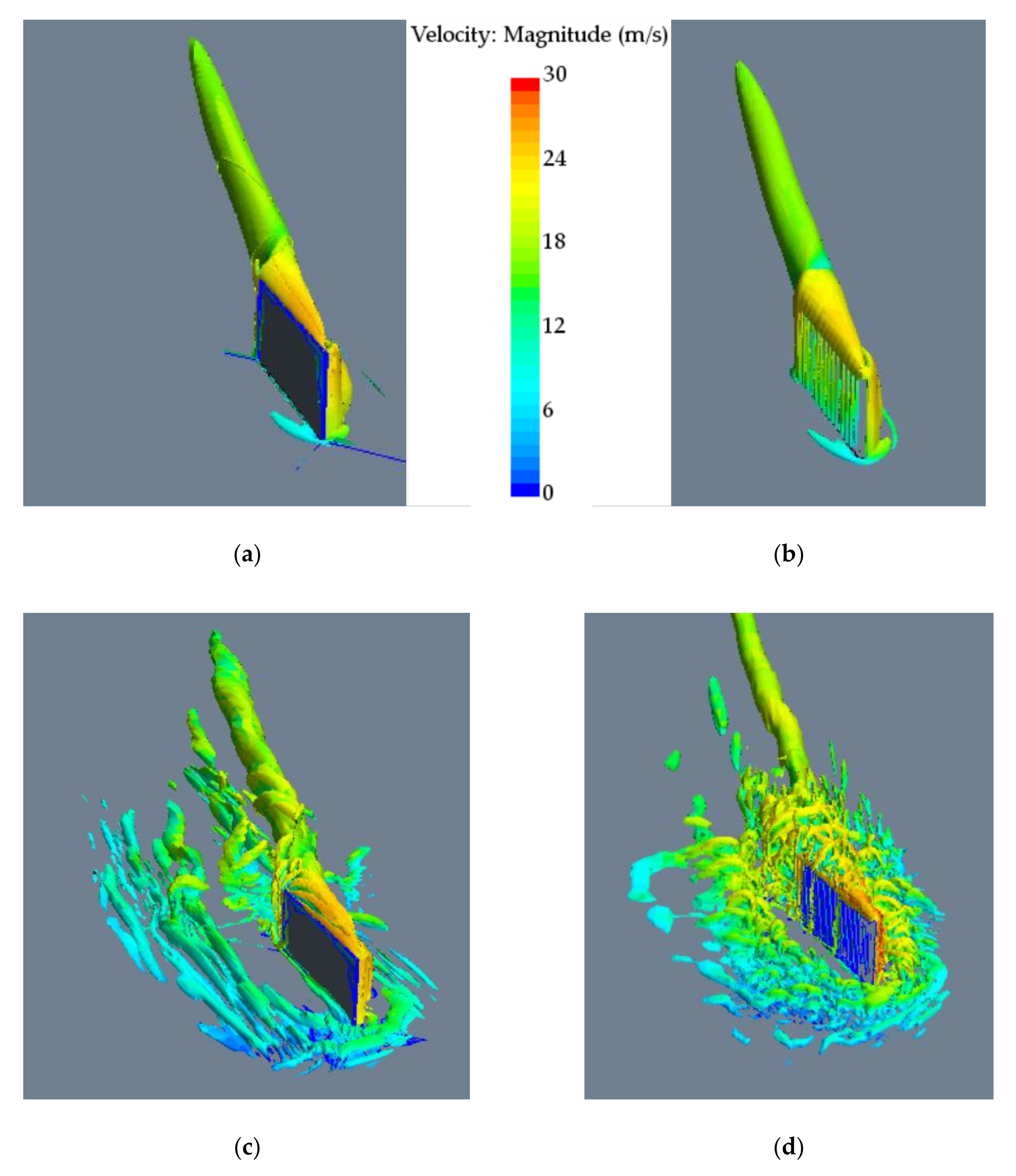
3.1. Coherent Structures

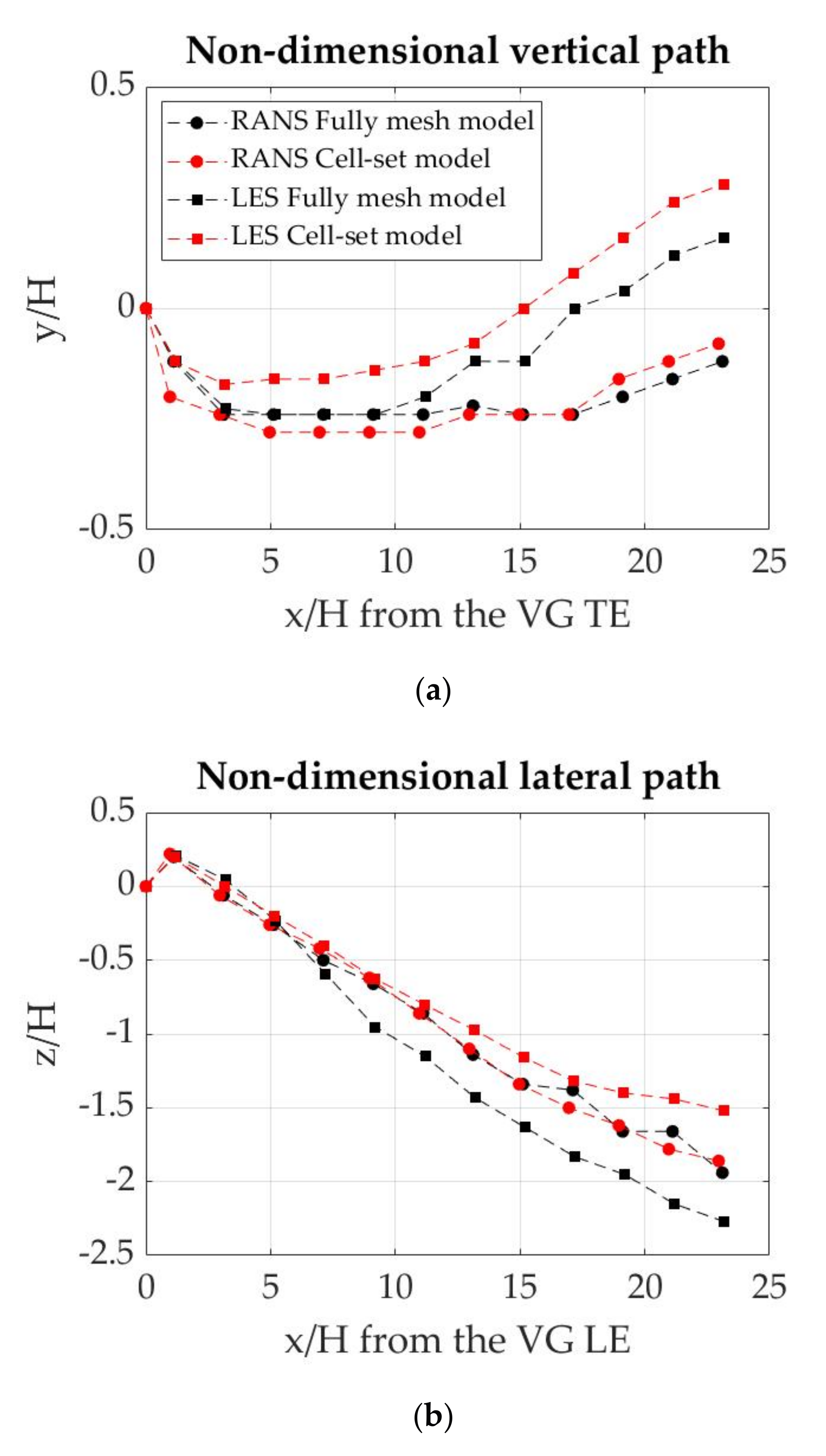
To identify the coherent structures of the flow, the Q-criterion method [30], represented by isosurfaces, is applied. The value of Q has been set at 2500 ${\mathrm{s}}^{-2}$. These isosurfaces can be shown in Figure 5.

Velte et al. [31] showed by PIV (Particle Image Velocimetry) measurements that two vortical structures appear in the wake behind the vane. The primary vortex appears at the top of the VG and follows the direction of the flow. The secondary vortical structure is a horseshoe vortex which appears at the lower part of the VG. This secondary vortex is divided into two sides, the pressure side and the suction side. As the suction side of the horseshoe vortex has the opposite sign to the primary vortex, at the early stage of its generation, the primary vortex sweeps the secondary vortex. Therefore, at the early stage of its generation, the secondary vortex does not follow the direction of the flow.

Both RANS simulations predict the primary vortex, but not the secondary one, and with both models similar predictions of the primary vortex are obtained.

In LES simulations, both the primary and the secondary vortex are predicted, but despite predicting the two vortical structures, the predictions of the cell-set model are not as good as those of the fully-resolved mesh model. The primary vortex predicted by the cell-set model is narrower and longer than the one predicted by the fully-resolved mesh model. In addition, the secondary vortex does not look as uniform as with the fully-resolved mesh model, so the pressure and suction side of the vortex are not accurately defined. Hence, the secondary vortex is not dragged by the primary vortex.

In both RANS and LES simulations with the cell-set model, small turbulences appear on the surface of the VG. These turbulences are attributed to the fact that the surface of the VG is not straight with this model.

3.2. Vortex Path

To analyze the vortexes, the axial velocity of the flow in the previously-mentioned 12 spanwise planes is considered. In RANS simulations, the instantaneous values are considered, whereas in LES simulations, the mean values of 2 s after the flow are fully developed. Figure 6 displays the axial velocities.

The results show that as the flow distances from the VG, the value of the axial velocity diminishes and the primary vortex grows. In accordance with Yao et al. [32], the shape of this vortex is not circular.

In RANS, similar results are obtained with the fully-resolved mesh model and the cell-set model, but in contrast with the coherent structures, the axial velocity shows the pressure side of the secondary vortex. In LES, as shown by the coherent structures, the primary vortex is narrower and the velocity in its center is bigger with the cell-set model, especially far from the VG.

Despite being similar in shape, the displacement of the primary vortex from the VG is not equal with both models. Hence, the position and trajectory of the primary vortex is studied. Figure 7 shows the vertical (Figure 7a) and lateral (Figure 7b) displacement of the center of the primary vortex (the point where the peak vorticity appears).

Near the VG, the vertical displacements show that the primary vortex center is located under the height of the VG, but as the flow displaces from the VG, the primary vortex goes up. This is more notable when α = 25°. With RANS, the vertical displacement near the VG is lower with the cell-set model, but it increases more as the flow distances from the VG. With LES, the trend is equal with both models, but slight differences in values are visible, being the vertical displacement of the cell-set model larger.

Regarding the lateral displacement, in all the cases the vortex center displaces flow the VG as the flow goes ahead. Near the VG, the displacements are very similar in both cases, but as the flow goes forward, the differences between models increase with LES. With RANS the results remain concordant along the whole path.

The results of both the vertical and lateral displacement are in accordance with the results obtained by Fernandez-Gamiz et al. [33].

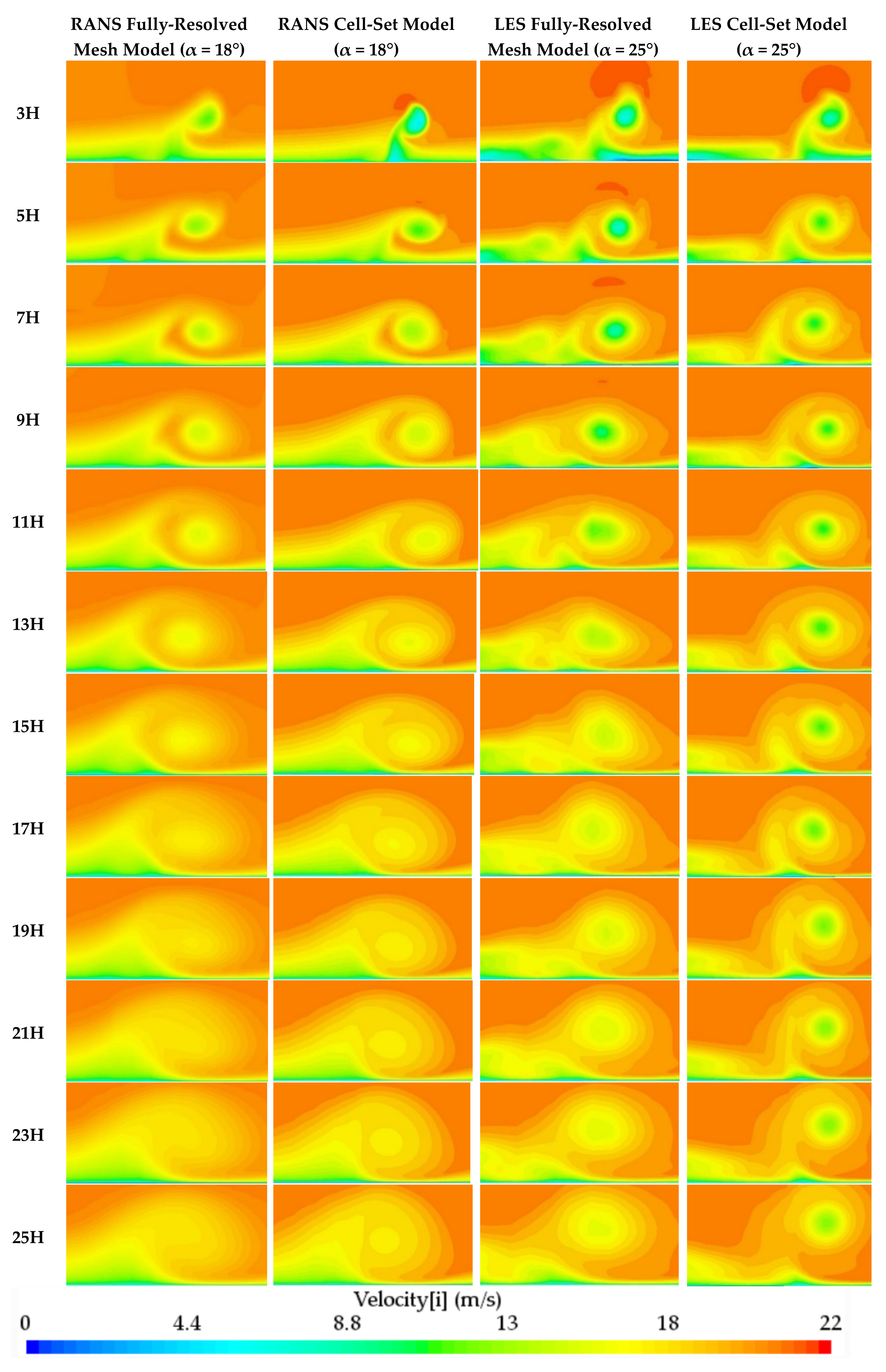
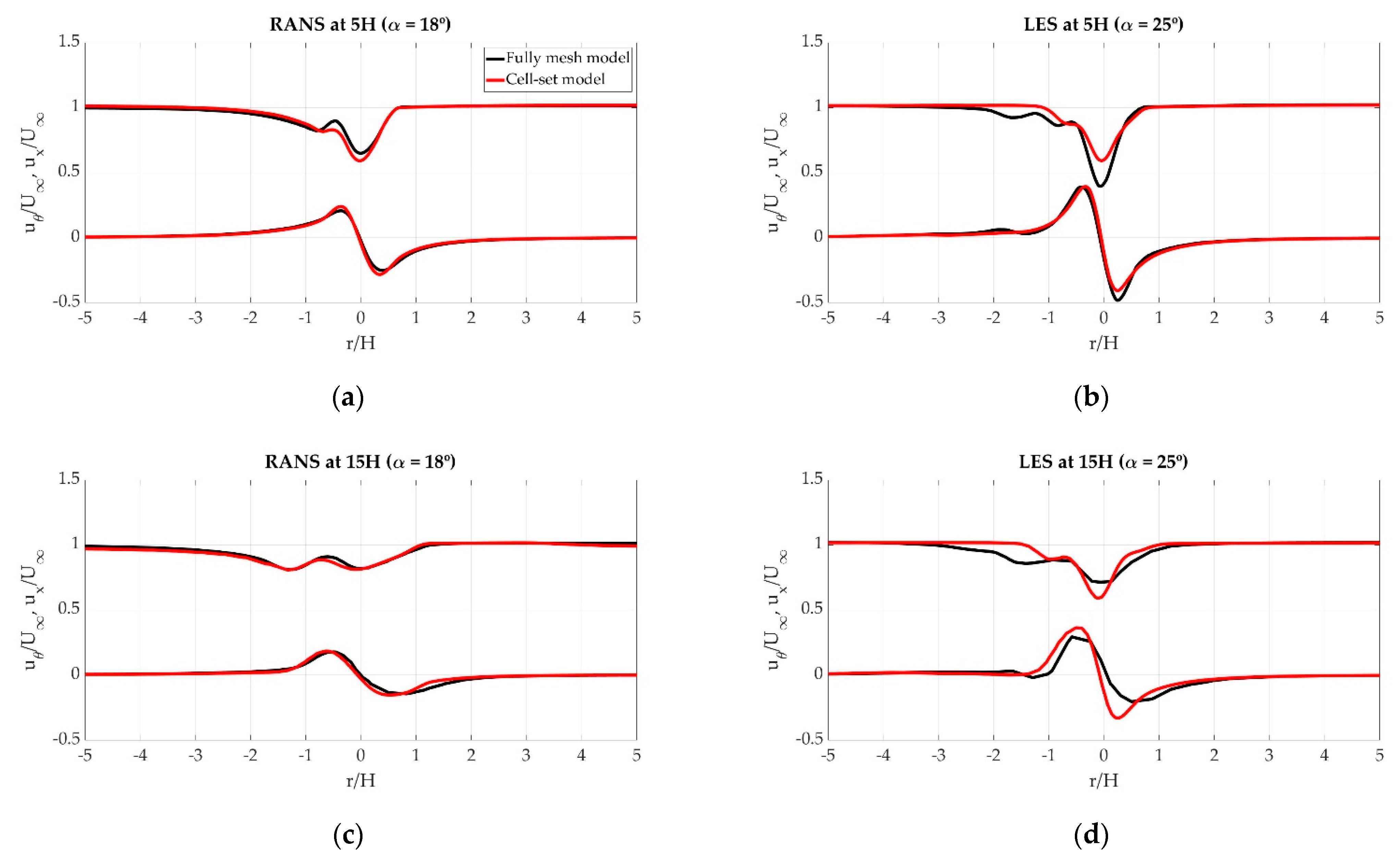
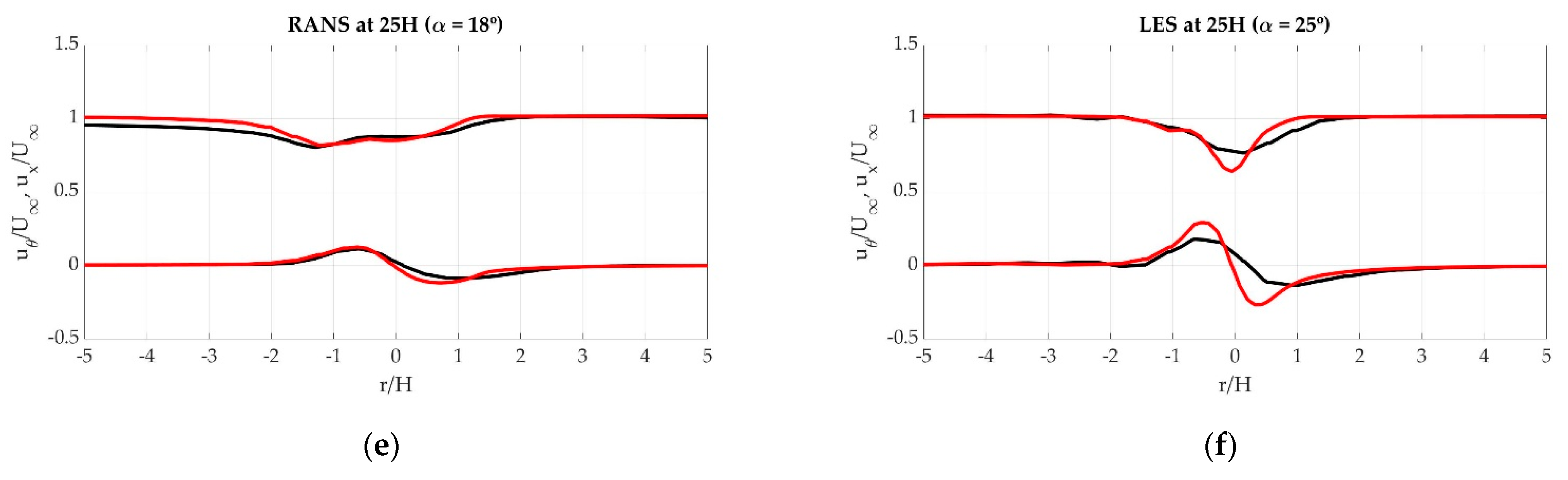
3.3. Velocity Profiles

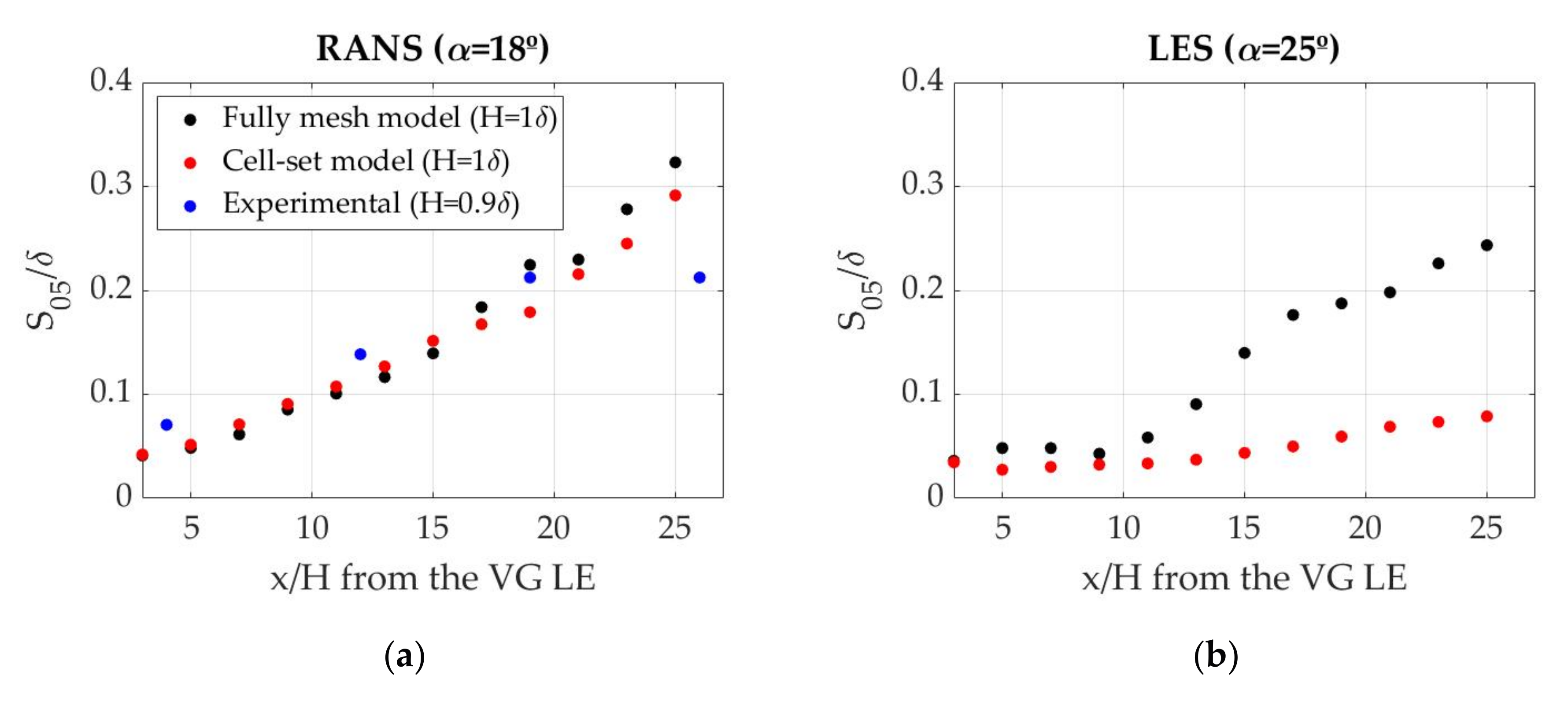
Velte et al. [34,35] showed that the primary vortex produced by a VG possess helical symmetry, and therefore the axial ($u_x)$ and azimuthal ($u_{\theta })$ velocity profiles are interrelated. To analyze the velocity profiles of the vortex, a horizontal line that crosses the center of the vortex is considered. Figure 8 shows the axial and azimuthal velocity profiles at 5H, 15H and 25H from the VG LE. These velocity profiles are normalized with the streamwise velocity.

The obtained velocity profiles describe the interrelation proposed by Velte et al. [34,35], but some disturbances are observed owing to the influence of the secondary vortex. The main disturbances are visible in the axial velocity profiles, which are not symmetric due to the influence of the pressure side of the secondary vortex.

In RANS, simulations almost equal to velocity profiles are obtained in the analyzed planes. In LES, though, despite obtaining similar results near the VG, bigger values of the velocity are obtained with the cell-set model, especially far away from the VG. However, the differences are relatively small, and the trend is almost the same.

3.4. Vortex Size

The Half-Life Surface ($S_{05}$) parameter introduced by Gutierrez-Amo et al. [36] is used in the present study to analyze the vortex size of the primary vortex. This parameter is an alternative to the Half-Life Radius ($R_{05}$) parameter developed by Bray [37] for cases where vorticity distribution is not symmetrical. This method consists of determining the elliptical-shaped area in which the vorticity value is greater than half of the peak value ($\omega >\frac{{\omega }_{peak}}{2}$). For that purpose, the vorticity distribution from points with the same spanwise coordinate as the vortex center is extracted to obtain the vorticity distribution normal to the flow direction. Then, four points are determined with a vorticity equal to $\frac{{\omega }_{peak}}{2}$. Finally, these four points are fitted to an elliptical shape. Figure 9 shows the $S_{05}$ values of the primary vortex. The results of $S_{05}$ are compared with the experimental results obtained by Bray [37]. Since in that study $R_{05}$ is analyzed, $S_{05}$ has been calculated from the $R_{05}$.

As expected, and in accordance with the results of the vortex path, the half-life surface increases as the flow distances from the VG. In accordance with the previously-obtained results, the half-life surface remains nearly constant with the cell-set model with LES. In RANS, the half-life surfaces are very similar with both models, and good agreements with experimental data are obtained, especially near the VG.

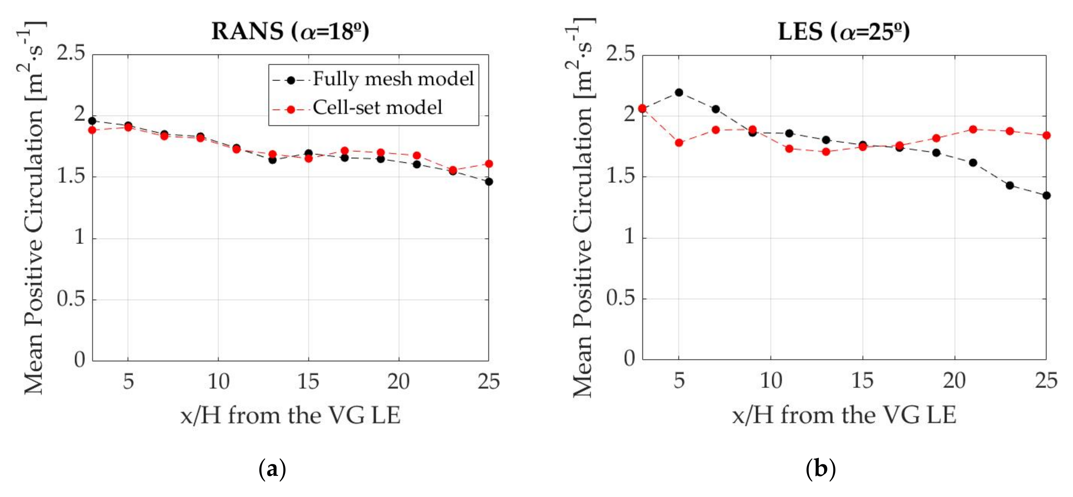
3.5. Vortex Strength

The capacity of spinning that the vortex acquires is evaluated with the positive circulation (${\Gamma }^{+}$) following this expression:

$${\Gamma }^{+}={{\displaystyle \int }}_S^{ }{\omega }_x^{+}dS$$

(2)

In this study, a parameter called mean positive circulation (${\Gamma }_{05}^{+}$) introduced by Gutierrez-Amo et al. [36] is considered. This parameter is an alternative to the positive circulation, with the fact that the previously-calculated $S_{05}$ parameter is required for its calculation, as defined in expression (3). Figure 10 displays the mean positive circulation of the primary vortex.

$${\Gamma }_{05}^{+}=\frac{{\omega }_{xmax}}{2}·S_{05}$$

(3)

As shown in the coherent structures, with LES, the primary vortex with the cell-set model is much longer than with the fully-resolved mesh model. This means that the vorticity is bigger and has resulted in larger values of the mean positive circulation far away from the VG. In addition, the values remain nearly constant, and therefore, barely diminish. In RANS, very small differences between models are found.

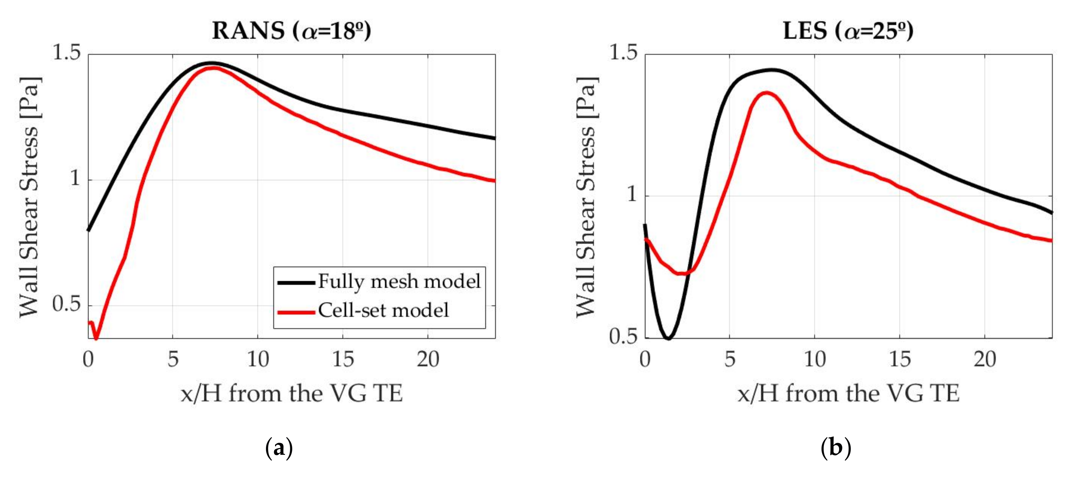
3.6. Wall Shear Stress

As mentioned above, the main target of VGs is to delay the flow separation. The wall shear stress is a significant parameter to understand this phenomenon. Figure 11 shows the wall shear stress values obtained behind the VG TE. In RANS simulations, the instantaneous values are considered, whereas in LES simulations, the mean values of 2 s after the flow is fully developed.

In all the cases, the wall shear stress goes from a low value to a maximum value, then decreases. This maximum value is obtained when x/H is around 7.

With both RANS and LES, accurate predictions of the location of the wall shear stress maximum value are obtained using the cell-set model, but the values are different. With RANS, the maximum values are nearly equal, but as the flow distances from the VG, the differences increase. With LES, in spite of following the same trend, the values are slightly lower in all the locations. These differences in values can be attributed to the displacement of the primary vortex, since the greater the displacement, the smaller the influence of the vortex behind the VG; and this leads to lower values of the wall shear stress. With both models, larger wall shear stress values are obtained when α = 18°. Since Godard and Stanislas [38] showed that the maximum skin friction appears when the angle of attack is near to 18°, these results were expected.

4. Conclusions

CFD simulations of a single VG on a flat plate in negligible streamwise pressure gradient conditions were performed with the fully-resolved mesh model and the cell-set model using RANS and LES turbulence models. The coherent structures, wall shear stress and path, size, strength and velocity profiles of the primary vortex were compared in order to evaluate the accuracy of the cell-set model. The implementation of the cell-set model has resulted in a decrease of cells from 11.5 million to 7.2 million, with savings of around the 40% in terms of computational time with both RANS and LES.

The results show a very good performance of the cell-set model using RANS-based turbulence models, since good agreements between the fully-resolved mesh model and the cell-set model in all the studied parameters were obtained.

With LES turbulence models, good predictions of the coherent structures, vortex path and wall shear stress were obtained using the cell-set model, but some discrepancies were obtained when analyzing the size, strength and velocity profiles of the primary vortex. All these differences appear because the cell-set model overpredicts the vorticity of the primary vortex when using LES, especially far away from the VG. Hence, vortex size predictions are lower, vortex strength predictions are higher and velocity profile predictions are higher in comparison with the fully-resolved mesh model. Nevertheless, except in the vortex size, where the disparities are considerable, the results are considered acceptable.

In conclusion, due to the good results obtained with RANS, the cell-set model is clearly suitable for RANS. With LES, the results are acceptable, but for the studied case, the fully-resolved mesh model outperforms the cell-set model. In any case, this is considered the first application of the cell-set model on VGs. Therefore, further research should be done to analyze the cases where the cell-set model provides more accurate results with LES, since this model can represent a great advantage over the fully-resolved mesh model due to the simulation time savings that its implementation entails.

References

1. Aramendia, I.; Fernandez-Gamiz, U.; Ramos-Hernanz, J.A.; Sancho, J.; Lopez-Guede, J.M.; Zulueta, E. Flow Control Devices for Wind Turbines. In Energy Harvesting and Energy Efficiency: Technology, Methods, and Applications; Bizon, N., Mahdavi Tabatabaei, N., Blaabjerg, F., Kurt, E., Eds.; Lecture Notes in Energy; Springer International Publishing: New York, NY, USA, 2017; pp. 629–655. ISBN 978-3-319-49875-1. [Google Scholar]
2. Aramendia-Iradi, I.; Fernandez-Gamiz, U.; Sancho-Saiz, J.; Zulueta-Guerrero, E. State of the art of active and passive flow control devices for wind turbines. DYNA 2016, 91, 512–516. [Google Scholar] [CrossRef] [Green Version]
3. Taylor, H.D. Summary Report on Vortex Generators. In Proceedings of the Research Department Report No. R-05280-9; Research Department, United Aircraft Corporation: Moscow, Russia, 1947. [Google Scholar]
4. Awais, M.; Bhuiyan, A.A. Heat transfer enhancement using different types of vortex generators (VGs): A review on experimental and numerical activities. Therm. Sci. Eng. Prog. 2018, 5, 524–545. [Google Scholar] [CrossRef]
5. Urkiola, A.; Fernandez-Gamiz, U.; Errasti, I.; Zulueta, E. Computational characterization of the vortex generated by a Vortex Generator on a flat plate for different vane angles. Aerosp. Sci. Technol. 2017, 65, 18–25. [Google Scholar] [CrossRef]
6. Fernandez-Gamiz, U.; Marika Velte, C.; Réthoré, P.-E.; Sørensen, N.N.; Egusquiza, E. Testing of self-similarity and helical symmetry in vortex generator flow simulations: Self-Similarity and helical symmetry in VG flow simulations. Wind Energ. 2016, 19, 1043–1052. [Google Scholar] [CrossRef]
7. Ibarra-Udaeta, I.; Errasti, I.; Fernandez-Gamiz, U.; Zulueta, E.; Sancho, J. Computational Characterization of a Rectangular Vortex Generator on a Flat Plate for Different Vane Heights and Angles. Appl. Sci. 2019, 9, 995. [Google Scholar] [CrossRef] [Green Version]
8. Martínez-Filgueira, P.; Fernandez-Gamiz, U.; Zulueta, E.; Errasti, I.; Fernandez-Gauna, B. Parametric study of low-profile vortex generators. Int. J. Hydrog. Energy 2017, 42, 17700–17712. [Google Scholar] [CrossRef]
9. Jirasek, A. Vortex-Generator Model and Its Application to Flow Control. J. Aircr. 2005, 42, 1486–1491. [Google Scholar] [CrossRef]
10. Bender, E.E.; Anderson, B.H.; Yagle, P.J. Vortex Generator Modelling for Navier-Stokes Codes; ASME Paper FED SM99-6919; ASME: San Francisco, CA, USA, 1999. [Google Scholar]
11. Ballesteros-Coll, A.; Fernandez-Gamiz, U.; Aramendia, I.; Zulueta, E.; Lopez-Guede, J.M. Computational Methods for Modelling and Optimization of Flow Control Devices. Energies 2020, 13, 3710. [Google Scholar] [CrossRef]
12. Chillon, S.; Uriarte-Uriarte, A.; Aramendia, I.; Martínez-Filgueira, P.; Fernandez-Gamiz, U.; Ibarra-Udaeta, I. jBAY Modeling of Vane-Type Vortex Generators and Study on Airfoil Aerodynamic Performance. Energies 2020, 13, 2423. [Google Scholar] [CrossRef]
13. Errasti, I.; Fernández-Gamiz, U.; Martínez-Filgueira, P.; Blanco, J.M. Source Term Modelling of Vane-Type Vortex Generators under Adverse Pressure Gradient in OpenFOAM. Energies 2019, 12, 605. [Google Scholar] [CrossRef] [Green Version]
14. Fernandez-Gamiz, U.; Réthoré, P.E.; Sørensen, N.N.; Velte, C.M.; Frederik, Z.; Egusquiza, E. Comparison of Four Different Models of Vortex Generators; European Wind Energy Association (EWEA): Copenhagen, Denmark, 2012. [Google Scholar]
15. Solís-Gallego, I.; Argüelles Díaz, K.M.; Fernández Oro, J.M.; Velarde-Suárez, S. Wall-Resolved LES Modeling of a Wind Turbine Airfoil at Different Angles of Attack. J. Mar. Sci. Eng. 2020, 8, 212. [Google Scholar] [CrossRef] [Green Version]
16. Bjerg, A.; Christoffersen, K.; Sørensen, H.; Hærvig, J. Flow structures and heat transfer in repeating arrangements of staggered rectangular winglet pairs by Large Eddy Simulations: Effect of winglet height and longitudinal pitch distance. Int. J. Heat Mass Transf. 2019, 131, 654–663. [Google Scholar] [CrossRef]
17. Saha, P.; Biswas, G.; Mandal, A.C.; Sarkar, S. Investigation of coherent structures in a turbulent channel with built-in longitudinal vortex generators. Int. J. Heat Mass Transf. 2017, 104, 178–198. [Google Scholar] [CrossRef]
18. Colleoni, A.; Toutant, A.; Olalde, G. Simulation of an innovative internal design of a plate solar receiver: Comparison between RANS and LES results. Sol. Energy 2014, 105, 732–741. [Google Scholar] [CrossRef]
19. STAR-CCM+ v2019.1. Available online: https://www.plm.automation.siemens.com/ (accessed on 2 June 2020).
20. Menter, F. Zonal Two Equation k-w Turbulence Models for Aerodynamic Flows. In Proceedings of the 23rd Fluid Dynamics, Plasmadynamics, and Lasers Conference; American Institute of Aeronautics and Astronautics: Orlando, FL, USA, 1993. [Google Scholar]
21. Smagorinsky, J. General circulation experiments with the primitive equations. Mon. Wea. Rev. 1963, 91, 99–164. [Google Scholar] [CrossRef]
22. Allan, B.; Yao, C.S.; Lin, J. Numerical Simulations of Vortex Generator Vanes and Jets on a Flat Plate. In Proceedings of the 1st Flow Control Conference; American Institute of Aeronautics and Astronautics: St. Louis, MO, USA, 2002. [Google Scholar]
23. Khosla, P.K.; Rubin, S.G. A diagonally dominant second-order accurate implicit scheme. Comput. Fluids 1974, 2, 207–209. [Google Scholar] [CrossRef]
24. Richardson, L.F.; Gaunt, J.A. The deferred approach to the limit. Philosophical Transactions of the Royal Society of London. Ser. A Contain. Pap. Math. Phys. Character 1927, 226, 299–361. [Google Scholar] [CrossRef]
25. Almohammadi, K.M.; Ingham, D.B.; Ma, L.; Pourkashan, M. Computational fluid dynamics (CFD) mesh independency techniques for a straight blade vertical axis wind turbine. Energy 2013, 58, 483–493. [Google Scholar] [CrossRef]
26. Stern, F.; Wilson, R.V.; Coleman, H.W.; Paterson, E.G. Verification and Validation of CFD Simulations; Defense Technical Information Center: Fort Belvoir, VA, USA, 1999. [Google Scholar]
27. Kuczaj, A.K.; Komen, E.M.J.; Loginov, M.S. Large-Eddy Simulation study of turbulent mixing in a T-junction. Nucl. Eng. Des. 2010, 240, 2116–2122. [Google Scholar] [CrossRef] [Green Version]
28. Tennekes, H.; Lumley, J.L. A First Course in Turbulence; MIT Press: Cambridge, MA, USA, 1972; ISBN 978-0-262-20019-6. [Google Scholar]
29. Kuczaj, A.K.; Komen, E.M.J. An Assessment of Large-Eddy Simulation toward Thermal Fatigue Prediction. Nucl. Technol. 2010, 170, 2–15. [Google Scholar] [CrossRef]
30. Hunt, J.C.R.; Wray, A.A.; Moin, P. Eddies, stream, and convergence zones in turbulent flows. Cent. Turbul. Res. Rep. CTR-S88 1988, 1, 193–208. [Google Scholar]
31. Velte, C.M.; Hansen, M.O.L.; Okulov, V.L. Multiple vortex structures in the wake of a rectangular winglet in ground effect. Exp. Therm. Fluid Sci. 2016, 72, 31–39. [Google Scholar] [CrossRef] [Green Version]
32. Yao, C.; Lin, J.; Allen, B. Flowfield Measurement of Device-Induced Embedded Streamwise Vortex on a Flat Plate. In 1st Flow Control Conference; American Institute of Aeronautics and Astronautics: St. Louis, MO, USA, 2002. [Google Scholar]
33. Fernández-Gámiz, U.; Zamorano, G.; Zulueta, E. Computational study of the vortex path variation with the VG height. J. Phys. Conf. Ser. 2014, 524, 012024. [Google Scholar] [CrossRef]
34. Velte, C.M.; Hansen, M.O.L.; Okulov, V.L. Helical structure of longitudinal vortices embedded in turbulent wall-bounded flow. J. Fluid Mech. 2009, 619, 167–177. [Google Scholar] [CrossRef] [Green Version]
35. Velte, C.M. A Vortex Generator Flow Model Based on Self-Similarity. AIAA J. 2013, 51, 526–529. [Google Scholar] [CrossRef] [Green Version]
36. Gutierrez-Amo, R.; Fernandez-Gamiz, U.; Errasti, I.; Zulueta, E. Computational Modelling of Three Different Sub-Boundary Layer Vortex Generators on a Flat Plate. Energies 2018, 11, 3107. [Google Scholar] [CrossRef] [Green Version]
37. Bray, T.P. A Parametric Study of Vane and Air-Jet Vortex Generators. Ph.D. Thesis, Cranfield University, College of Aeronautics, Bedford, UK, 1998. [Google Scholar]
38. Godard, G.; Stanislas, M. Control of a decelerating boundary layer. Part 1: Optimization of passive vortex generators. Aerosp. Sci. Technol. 2006, 10, 181–191. [Google Scholar] [CrossRef]
Figure 1. (a) Computational domain (not to scale). (b) Vortex Generator (VG) dimensions.
Jmse 08 00982 g001aJmse 08 00982 g001b
Figure 2. Refined mesh near the VG.
Jmse 08 00982 g002
Figure 3. Mesh verification for Large Eddy Simulation (LES): (a) Autocorrelation functions; (b) Taylor length scale and mesh resolution.
Jmse 08 00982 g003
Figure 4. Cell-set construction of the VG with the cell-set model. (a) α = 18°; (b) α = 25.
Jmse 08 00982 g004
Figure 5. Isosurfaces colored by velocity: (a) Reynolds-Averaged Navier-Stokes (RANS) Fully-Resolved Mesh (α = 18°); (b) RANS Cell-Set Model (α = 18°); (c) LES Fully-Resolved Mesh (α = 25°); (d) LES Cell-Set Model (α = 25°).
Jmse 08 00982 g005
Figure 6. Axial velocity at 12 different spanwise planes.
Jmse 08 00982 g006
Figure 7. Non-dimensional trajectory of the primary vortex: (a) Non-dimensional vertical path; (b) Non-dimensional lateral path.
Jmse 08 00982 g007
Figure 8. Normalized axial (upper) and azimuthal (lower) velocity profiles: (a) RANS at 5H from the VG Leading Edge; (b) LES at 5H; (c) RANS at 15H; (d) LES at 15H; (e) RANS at 25H; (f) LES at 25H.
Jmse 08 00982 g008aJmse 08 00982 g008b
Figure 9. Half-Life Surface of the primary vortex: (a) RANS; (b) LES.
Jmse 08 00982 g009
Figure 10. Mean positive circulation of the primary vortex: (a) RANS; (b) LES.
Jmse 08 00982 g010
Figure 11. Wall shear stress behind the Trailing Edge (TE) of the VG: (a) RANS; (b) LES.
Jmse 08 00982 g011