Performance Assessment of ERA5 Wave Data in a Swell Dominated Region


Department of Civil, Environmental, Building Engineering and Chemistry, Polytechnic University of Bari -Via E. Orabona, 4, 70125 Bari, Italy
*
Author to whom correspondence should be addressed.
J. Mar. Sci. Eng. 2020, 8(3), 214; https://doi.org/10.3390/jmse8030214
Submission received: 18 February 2020
/
Revised: 7 March 2020
/
Accepted: 15 March 2020
/
Published: 19 March 2020
(This article belongs to the Section Ocean Engineering)
Abstract
:The present paper deals with a performance assessment of the ERA5 wave dataset in an ocean basin where local wind waves superimpose on swell waves. The evaluation framework relies on observed wave data collected during a coastal experimental campaign carried out offshore of the southern Oman coast in the Western Arabian Sea. The applied procedure requires a detailed investigation on the observed waves, and aims at classifying wave regimes: observed wave spectra have been split using a 2D partition scheme and wave characteristics have been evaluated for each wave component. Once the wave climate was defined, a detailed wave model assessment was performed. The results revealed that during the analyzed time span the ERA5 wave model overestimates the swell wave heights, whereas the wind waves’ height prediction is highly influenced by the wave developing conditions. The collected field dataset is also useful for a discussion on spectral wave characteristics during monsoon and post-monsoon season in the examined region; the recorded wave data do not suffice yet to adequately describe wave fields generated by the interaction of monsoon and local winds.
1. Introduction
Numerical models provide continuous and reliable meteomarine datasets in space and time in open oceans [1,2] commonly used to assess wind and wave climatology, and long term analysis related climate change’s effects upon the wave climate. Meteo-marine models are an essential element in coastal zone management in the early identification of critical areas [3,4], the analysis of evolutive trends [5] and, at a higher level, the definition of medium and long-term effective strategies for environmental/territorial planning [6]. In the last few decades, several global-scale wave atlases have been proposed using wave datasets from global wave models [7,8,9], highlighting the presence of stormy areas (i.e., Northwest Pacific, Northwest Atlantic, Southern Ocean and Mediterranean Sea), and swell-dominated regions termed ”swell pools” located in the eastern tropical areas of the Pacific, the Atlantic and the Indian Ocean.
On the other hand, the performances of wind and wave forecasting models depend on several variables. Among them it is worth citing the wave developing conditions. Past studies analyzed wave datasets from the European Centre for Medium-Range Weather Forecasts (ECMWF) and outlined underestimation in areas with intense cyclone activity and fetch-limited conditions and overestimation in swell-dominated regions [2]. In general, wave data reliability is below acceptable levels when coastal areas and enclosed basins with local wind influence and with orographic and bathymetric effects are considered [10]. Indeed, in a semi-enclosed basin as the Mediterranean Sea, where fetch limited conditions are predominant, wave heights are often underestimated [11,12]. In a different context, such as the North Indian Ocean where swells are predominant, the comparison between observed and modeled wave heights revealed a wave height overestimation in nearshore waters due to swell presence, except during the Indian monsoon wind season when a large underestimation can be detected [13].
Hence, wave observing programs that at first glance could appear out of date, unnecessarily elaborate or expensive, still need to be carried out to perform numerical wave model calibration and develop data-driven models [14,15,16], and to describe global wave climate [17,18] and local wave characteristics [19,20,21,22]. Of course, all available observing wave data sources suffer from a variety of problems depending on the data acquisition system. Measured waves typically show a good accuracy, but are limited by the number of instruments and the duration of the measurement campaign (wave buoys), or can be very time sparse, presenting reliability concerns in coastal zones (remote sensing techniques). Wave data from observing voluntary ships are also available, but datasets are sparse, not continuous and are clustered along the busiest sea routes. Modeled and observed data are complementary, and combined use ensures the best possible results in wave analysis [12].
The aim of the present work is to assess the ECMWF ERA5 Re-Analysis dataset’s performance in a coastal region where wind and swell waves are both present. ERA5 is the latest global atmospheric reanalysis, and in the next few years the dataset will cover the period from 1950 to near real time [23]. ERA5 wave data have been compared to an observed wave dataset collected within the frame of a coastal experimental campaign carried out offshore of the Oman coast in the western Arabian Sea, where the wave climate is swell dominated (Figure 1).
This paper is structured as follows: after the introduction of the study area, a detailed description of the examined dataset and the methodologies used is presented in Section 2. Section 3 presents the results of the wave spectral analysis and the ERA5 wave model comparison, and conclusions are given in Section 4.
2. Materials and Methods
2.1. Case Study and Data Sources
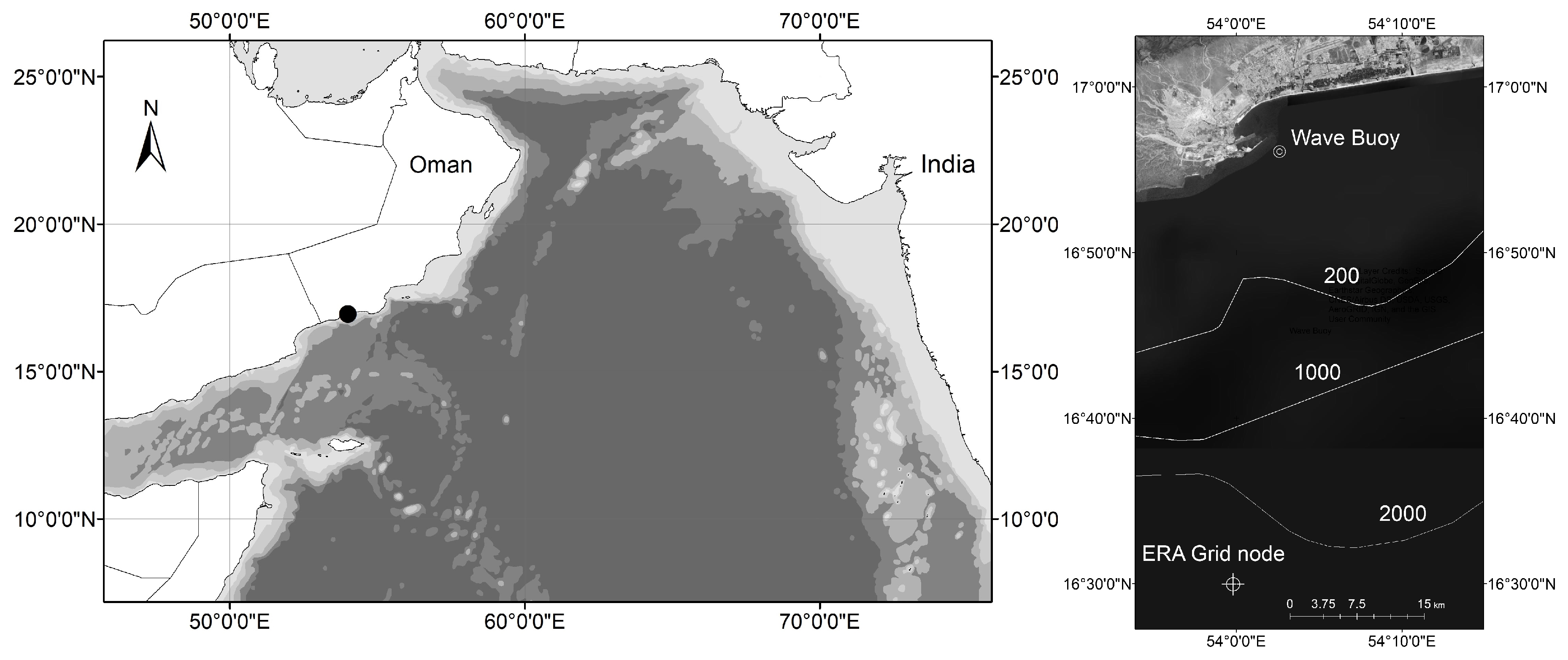
The Arabian Sea is connected with the Indian Ocean. It is one of the most important navigation routes in the world, bounded in the west by Somalia and Arabia and in the east by India (Figure 2—left image). The wind field offshore southern Oman coast is quite complex: high-resolution modeled wind fields revealed, also, the presence of the Oman coastal low-level jet clearly distinguished from the large-scale South Asia monsoon wind and the Somali jet [24]. Although Oman is one of the most arid countries in the world, the southern Oman coast (Dhofar region) enjoys a cooler temperature and misty rain from June to September (the so-called Khareef season) due to the SW monsoon. The southern Oman climate is strongly influenced by the Indian monsoon, and three different anemometric seasons can be detected: pre-monsoon (from February to May), southwest (SW) monsoon (from June to September) and post-monsoon or northeast (NE) monsoon (from October to January) [25].
Additionally, the wave climate in the region is influenced by the SW monsoon with wave heights gradually increasing from June, reaching a peak during July and gradually decreasing until the end of the Khareef [26]. Infra-gravity waves that cause a large shipping surge and reduce cargo shipments during the summer season have been widely reported [26,27]. Very few wave data are available in the western Arabian Sea, and general features of weather and wave conditions can be inferred from the wave analysis performed on wave data recorded offshore the west coast of India. To date, several buoys, moored along the eastern Arabian Sea, provide useful real-time information about weather and wave climate across that region. During the SW monsoon season, the sea state across the North Indian Ocean is dominated by swells, which come from SW directions and an increase in the significant height can be observed [28]. Wave spectra in shallow water, recorded in two different sites from June to October, are single peaked, while in the rest of the year double peaked spectra are the most frequent [29,30]. Although both sites are subject to open sea conditions, the percentage of single peaked spectra was greater in the south compared to the northern site due to local wind. Throughout the year, at the southernmost point, the double peaked spectra were predominantly dominated by swell waves. All over the years, from June to August, wave spectrum is narrow banded and energy density is concentrated predominantly between 0.07–0.12 Hz. During September, the wave energy density is predominantly between 0.09–0.14 Hz (11 s and 7 s).
During the winter season (post-monsoon and at the beginning of the pre-monsoon period) Shamal events occur (wind coming from the north) [25,29]. During these events, there is a sharp increase in wave height that may exceed 3.5 m in the northwestern Arabian Sea and 1.0–2.0 m along the west coast of India. Although south swells from the Indian Ocean are always present along the west coast of India, Shamal events are the main contributor to the sea states [31].
Wave analysis during the non-monsoon season revealed a daily variation of the wave parameters due to the coexistence of waves coming from different directions with a predominance of mature swell [31,32].
In the last few years, there has been rapid development along the southern coast of Oman. In particular, the traffic in the port of Salalah, a large container transshipment terminal, has rapidly increased, thanks to continuous improvement of its infrastructure. The absence of a meteomarine monitoring network and the lack of regular and long-term observations is still an important issue in coastal protection and harbor planning, especially in such a complex environment. In order to overcome the lack of observed wave data, and from the perspective of the development of the harbor, an experimental campaign was carried out in the second half of 2013 to collect detailed information about wave climate offshore the harbor facilities, water levels and sea currents. A Datawell Directional Waverider MKIII buoy was moored offshore Port Salalah (Figure 2) from early August 2013 through late December 2013, partially covering the southwest monsoon season in 2013. The geographical coordinates of the buoy are 1656′6.13″ N and 542′36.21″ E with a local depth of 30 m (Figure 2-right image). The sensor consists of a Datawell stabilized platform sensor, performing heave and direct pitch and roll measurements combined with a 3D fluxgate compass and X/Y accelerometers at 1.28 Hz. The buoy measures wave height for wave periods of 1.6 to 30 s with an accuracy equal to 0.5% of measured value.
The wave buoy installation and data management was carried out by a research team that included the unit of the Laboratory of Coastal Engineering (LIC) of the Polytechnic University of Bari. The collected dataset allows to obtain local information on the wave climate and a comparison with the eastern Arabian Sea wave climate that also experiences the SW monsoon. The observed dataset covers a five-month period and therefore it does not suffice to define the wave climate of the region. Nevertheless, the data are useful for a discussion about spectral wave characteristics during monsoon and post-monsoon period and for numerical wave data validation purpose (i.e., extracted from ERA5 dataset). Indeed, although the predominant swells from the south Indian Ocean may have similarities with the west Indian coast, the wave field offshore Dhofar region is influenced by local wind patterns.
Given the lack of previous studies reporting sea state conditions along the examined coast and in the wider region, in order to characterize the wind and wave patterns offshore Salalah and across the Arabian Sea, ERA5 Re-Analysis dataset from ECMWF has been used. The ERA5 wave dataset is produced using 4D-Var data assimilation in ECMWF’s Integrated Forecast System (IFS) Cycle 41r2 [33,34]. The ERA5 dataset compared to ERA-Interim wave data [35] presents several improvements including much higher spatial and temporal resolution, information on variation in quality over space and time, much improved troposphere and an improved representation of tropical cyclones [34]. The ERA5 dataset also provides uncertainty information obtained from data assimilation and an enhanced number of output parameters. The horizontal resolution of the wave model in ERA5 is 0.36 degrees; the wave dataset derived from the global re-analysis consists of instantaneous forecast values computed every 1 hour with a horizontal resolution of approximately 0.5 degrees, whereas ERA-I wave dataset provides 6 hourly data at 1 degrees spatial resolution. Significant wave height of combined wind waves and swell (SWH), mean wave period (MWP), mean wave direction (MWD), significant height of wind waves (SHWW) and significant wave height of total swell (SHTS) have been extracted at the nearest grid point offshore the area of interest (16.5 N, 54 E), about 50 km offshore the wave buoy. The wave parameters are listed in the Appendix A.
2.2. Spectral Analysis and Partition Schemes
Half-hourly raw elevation data (heave, pitch and roll) have been analyzed and directional and frequency spectra have been obtained. Frequency spectra have been obtained by means of standard Fast Fourier Transform (FFT) to heave time series. Significant wave height () and mean wave period () have been computed from 1D spectral moments and peak period () as the inverse of the spectral peak frequency. Directional wave spectra have been computed through Maximum Likelihood Method (MLM) [36] with a resolution of 0.005 Hz in frequency and 3.6 in direction. Mean wave direction (MWD) and directional spread (), which can be seen as the mean and standard deviation of the directional distribution function, respectively, have been estimated by using the method proposed by [37].
In addition to frequency domain analysis, a standard zero-up crossing analysis has been also performed in the time domain, defining individual waves and wave height and period distribution [38].
Several other spectral parameters have been evaluated to describe the shape and the type of recorded spectra. The spectral parameters are listed in the Appendix A. The spectral narrowness parameter [39] and the spectral width parameter [40] have been estimated in order to measure the width of the spectral band. The dimensionless parameters and can vary between 0 (narrow band) and 1 (broadband). The spectral peakedness parameter was proposed by [41] to describe the peakedness of the spectral peak and the wave groupiness. According to [42] has been recognized to be a appropriate parameter to describe spectral distribution, since it does not depend on the cut-off frequency unlike and . The significant spectral steepness is defined as the ratio between and deep water wavelength that corresponds with wave period. According to [43], waves depending on significant steepness values can be classified as wind wave (0.08–0.025), young swell (0.025–0.01), mature swell (0.01–0.004) and old swell (<0.004). So far, various techniques have been developed for spectral partitioning. They can be classified into 1D and 2D methods, depending on whether or not they use directional spectral information [44]. Directional spectra provide additional information about different wave systems that compose irregular sea states and 2D partitions methods seems to be more reliable in the wind wave and swell detection [45]. In the present work, swell and wind wave separation and detection have been performed exploiting image processing techniques to deal with 2D spectrum information [45]. Directional spectra have been smoothed to remove noise using a 3 × 3 convolution filter and then a watershed algorithm has been applied to separate the existing wave systems. The smoothing and spectral segmentation is an iterative process that continues until the number of spectral partitions reaches the maximum allowed number (usually 4–6). The detected wave systems have been then classified as wind seas or swell [46] comparing the 1D spectrum energy value at the peak frequency of a wave system to the energy spectrum estimated according to Pierson-Moskowitz spectrum [47,48] at the same peak frequency . If the ratio is greater than 1 the wave system is classified as wind wave, otherwise the wave system is swell. Eventually, wave characteristics have been calculated for each wave system. Swell and wind wave series resulting from watershed partitioning have been compared to results obtained with wave age method [49]. Wave age method, unlike the method proposed by [45], requires wind information to identify different wave regions in a directional spectrum, limiting its application. Indeed, synchronous wave and wind data are not usually available. Moreover, for further check of spectral partitioning, separation frequency of wind waves from swell in 1D spectra has also been calculated using the spectrum integration method [50]. The last approach is an improvement of the wave steepness method [51], that has been proven to overestimate wind waves under light wind when a significant swell is present [45].
Wind wave and swell wave characteristics have been estimated from partitioned 1D spectra and temporal variability have been analyzed.
2.3. Performance Evaluation of ERA-I and ERA5 Wave Datasets
The ability of ERA-I and ERA5 wave model to simulate significant wave heights and mean wave periods has been assessed. The assessment is useful to gain insight about the reliability of ERA-I and ERA5 data in regions where both swell and wind waves are present. The validation framework relies on the use of goodness-of-fit parameters and their statistical significance [52]. A model performance assessment based on a single indicator could lead to incorrect verification of the model, because all goodness-of-fit parameters are affected by limitations [53,54].
The coefficient of determination , defined as the square of the correlation coefficient, is the most widely used parameter to assess the predictive accuracy of models. Nevertheless, it is insensitive to additive and proportional differences between the model simulations and observations. The Nash-Sutcliffe coefficient of efficiency (NSE), defined as the ratio of the mean square error to the variance in the observed data subtracted from unity, can be seen as an improvement of . Indeed, it is sensitive to differences in the observed and model simulated means and variance. However, both coefficients are extremely sensitive to outliers. The coefficient of determination ranges from 0.0 to 1.0, whereas NSE ranges from minus infinity to 1.0. The Nash-Sutcliffe coefficient of efficiency values lower than zero indicate that the observed mean is a better predictor than the model. The higher the values of the above mentioned coefficients, the better the agreement. Although NSE values interpretation depends on model applications and can be subjective, ref. [52] proposed four model performance classes, which are rated as unsatisfactory (NSE ≤ 0.65), acceptable (NSE = 0.65–0.8), Good (NSE = 0.8–0.9) and very good (NSE ≥ 0.9).
Circular statistical parameters (i.e., RMSE, bias) have been estimated for observed and predicted wave directions. The relationship between the direction of modeled and observed waves has been analyzed using a circular correlation coefficient () as proposed by [55] for two circular random variables. The value of takes values within the interval from −1.0 to 1.0, where zero indicates that there is no relationship between the variables and represents the strongest correlation possible. The “goodness-of-fit” parameters are listed in the Appendix A, where N is the number of observations, while and are the observed and simulated, respectively.
3. Observed Data Analysis
The procedure, illustrated in Figure 1, has been applied to the buoy observed dataset. After a preliminary processing of the raw data, a spectral partitioning was carried out using different methods in order to determine the best spectral splitting technique under such wave conditions. Then, the observed sea states were classified as swell and wind waves.
3.1. Wave Characteristics
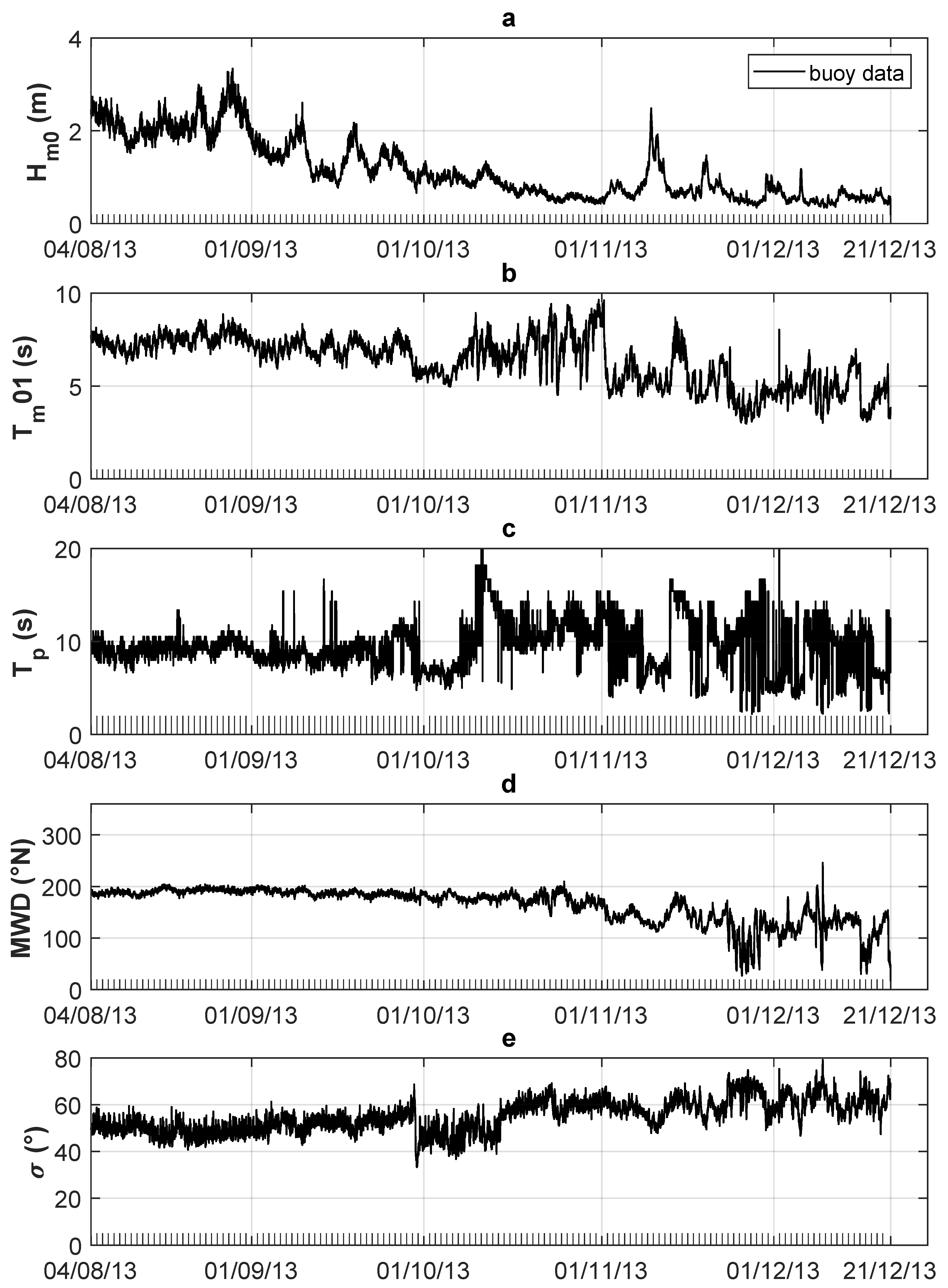
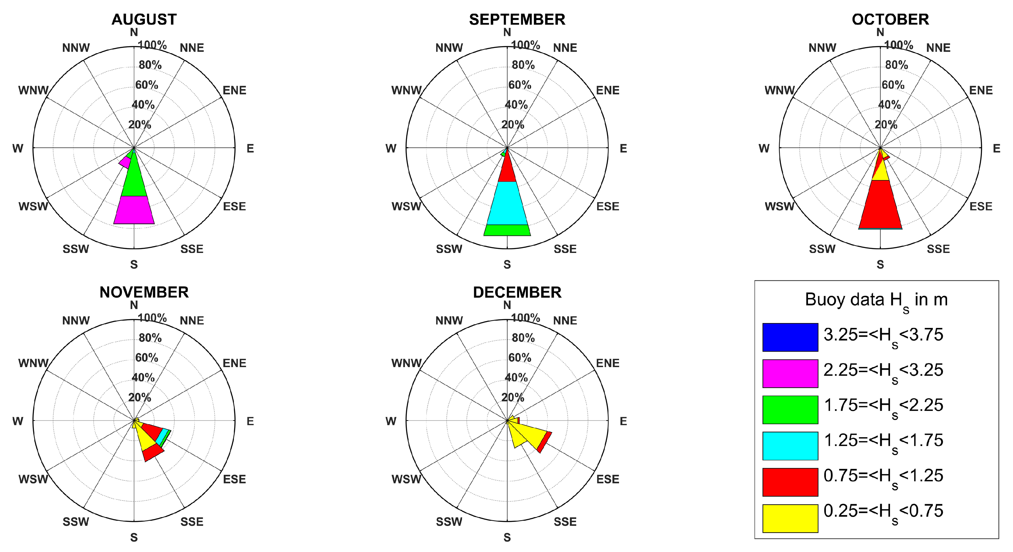
Series of significant wave height (), peak wave period (), mean wave period (), mean wave direction (MWD) and directional spread parameter () have been obtained over 30-min intervals (Figure 3). and the distribution of the percentage frequency of wave direction and height has been analyzed for different months (Figure 4). The buoy was exposed to waves approaching from 55 to 235. As highlighted by [56], the SW monsoon in 2013 presented some peculiarities—a very fast onset and a slower withdrawal phase that lasted from early September until the third week of October. This pattern can be detected in the recorded wave time series from offshore southern Oman. There is a clear distinction between the SW monsoon period (August), characterized by the highest waves coming almost exclusively from the south, and the post-monsoon period (from November to December), characterized by waves coming from east-southeast (ESE) and south-southeast (SSE). In that period, NE monsoon wind waves coexist with long-traveled southern swells, and these two wave systems result in a wave field with MWD tending to SE. The months of September and October 2013 can be seen as a transitional period with low waves coming from S. In August, about 60% of significant wave heights are between 2.25 m and the 3.25 m, while the remaining 40% are within the range 1.75 m and 2.25 m. In September, the direction from which the 92% of the waves come from is south. Waves from SSW constitute the remaining 8%. The wave height values, in this month, are always lower than 2.25 m. Significant wave height values (Figure 3a) decrease from the monsoon period to the post-monsoon period (usually below 1.5 m). The only significant sea storm in the post monsoon was generated by the 2013 Somalia cyclone that severely affected the Oman coast on November.
During the monsoon period, spans the range 5–8.5 s, while in the post-monsoon period has a wider range (3–10 s) (Figure 3b). When analyzing the wave peak periods (Figure 3c), it is observed that the values are between 5 s and 15 s in the monsoon period. On the other hand, the values belong to a wider range (between 3 and 20 s) in the post-monsoon period. In monsoon period, higher values of the significant wave height are consistent with the observed lower variability of the values.
Looking at directional spread parameter () (Figure 3e) a wider range of values can be observed in the post-monsoon season.
Wave parameters estimated using zero up-crossing analysis are listed in Table 1. The maximum value of in the monsoon period reaches about 6 m. It can be noted that the average valuse of and in the monsoon period are about 2.5 times larger than the values in the post-monsoon period. Regarding the wave period during the monsoon season, is higher with a smaller variability range than in the post-monsoon period.
3.2. Wave Spectra
Wave spectra and spectral shape parameters have been estimated and their temporal evolution during the recorded period has been analyzed.
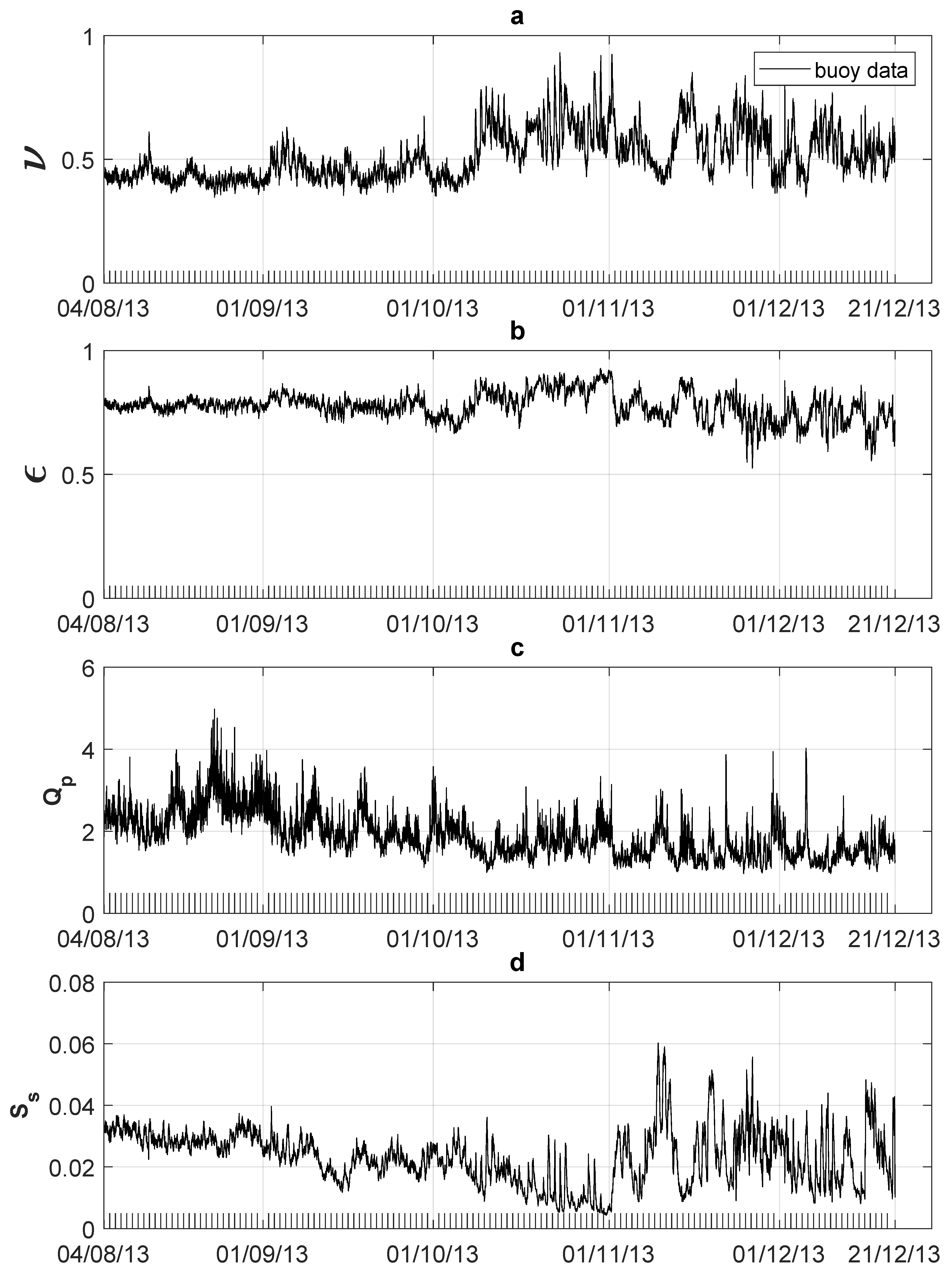
The estimated spectral narrowness (Figure 5a) varies, during the monsoon season, between 0.35 and 0.65, while greater values have been detected during the post-monsoon period. Narrowness values are in agreement with values obtained for the monsoon period in the Arabian Sea along the western coast of India [29]. Differently, spectral width values for narrow-banded spectra in the monsoon period are higher than the values found in broad-band spectra in the post-monsoon: this parameter cannot be used as an indicator for the spectral width (Figure 5b). The spectral peakedness parameter [41], instead, seems to be useful for spectral narrowness estimation, with higher values during the monsoon period and lower values for broad band spectra in the post-monsoon (Figure 5c).
The significant spectral steepness decreases going from monsoon period to the post-monsoon (Figure 5c). In the SW monsoon period, the waves can be classified as either young swells or wind waves, with steepness values between 0.01 and 0.03. In the post-monsoon period, the steepness values are in a wider range between 0.005 and 0.033, and swells, young swells and wind waves can be detected.
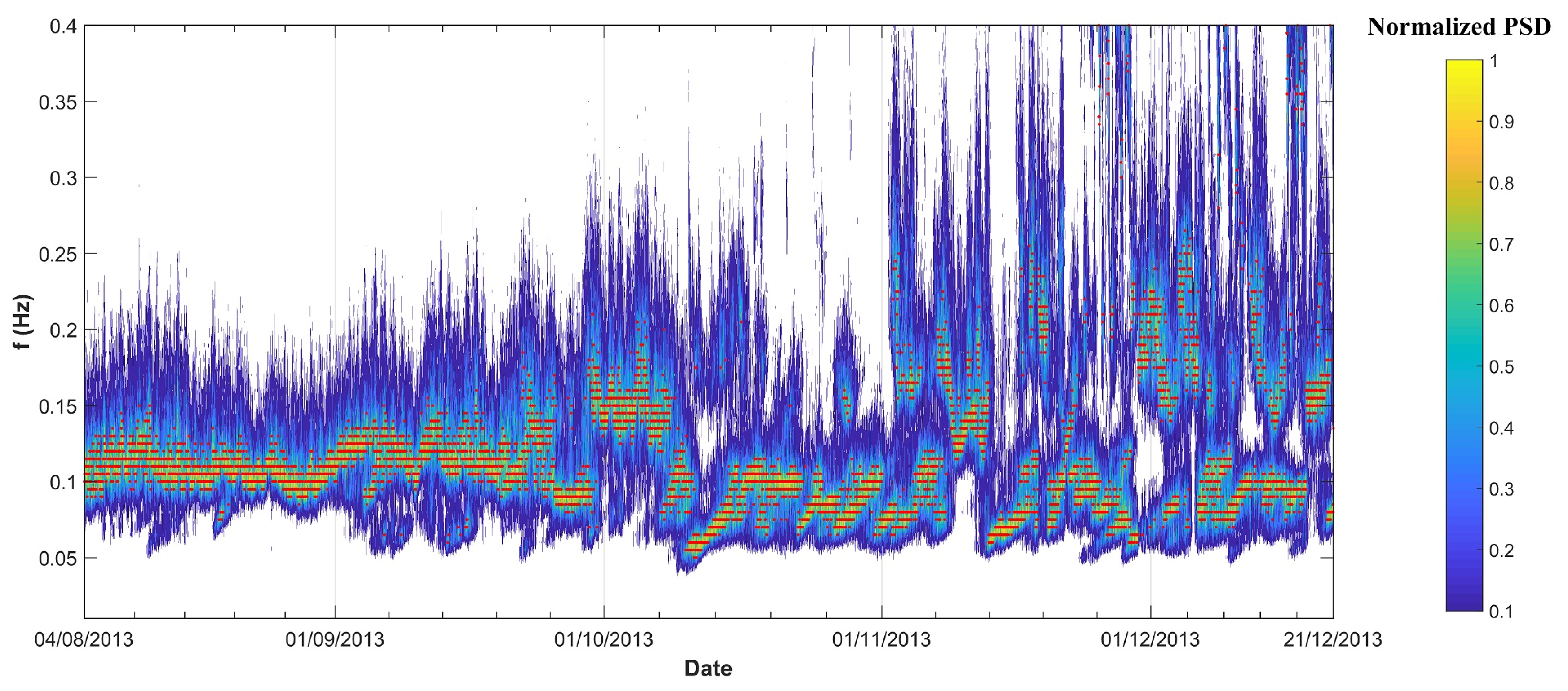
Figure 6 shows temporal variability of normalized spectral energy density. To obtain the normalized spectral energy value, energy density corresponding to a given frequency has been compared to the peak energy density. The highest values of normalized energy density are found at frequencies between 0.08 and 0.13 Hz (period between 12.5 and 7.7 s) from August to September, whereas are between 0.05 and 0.3 Hz in the post-monsoon period (corresponding period between 3.5 s and 20 s) when wind waves coexist with long swell waves, as can be seen from Figure 7.
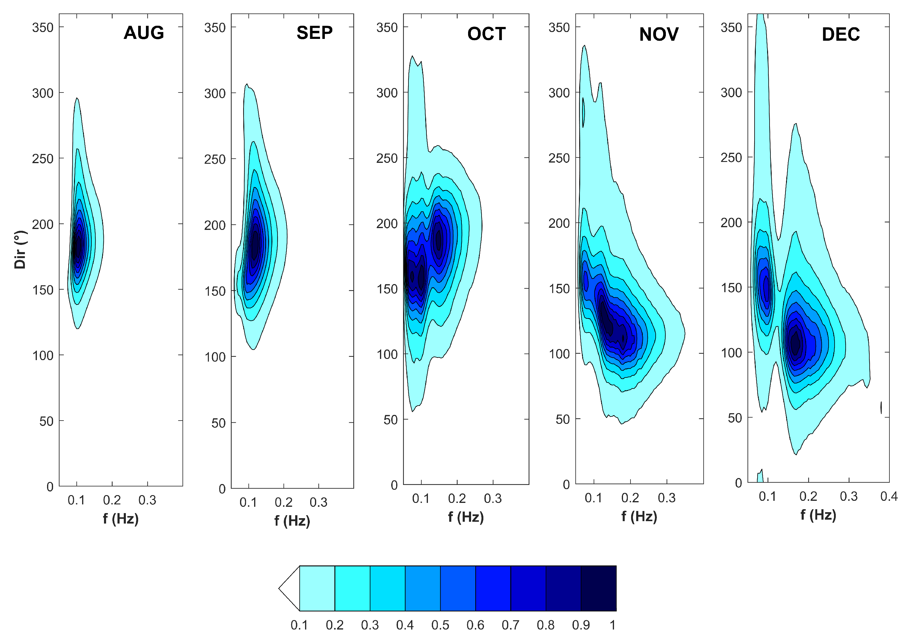
The average monthly directional spectra have been obtained by averaging semi-hourly recorded spectra. To obtain normalized spectral energy value, energy density corresponding to a given frequency has been compared to the peak energy density. Looking at the temporal variability from August to December, it can be noted that the monthly averaged spectrum tends to flatten going from the monsoon period to the post-monsoon evolving from an almost unimodal shape in August to spectra with very low energy density and multiple peaks during post-monsoon (Figure 7). This is consistent with [30]; they observed the same behavior along the western Indian coast. In August average monthly directional spectra have the highest spectral density with a peak period at 0.1 Hz and wave direction at about 180. In September, frequency bands are significantly wider than in August and the wave direction varies between 100 and 300. In October, multipeaked spectra appear and three different wave systems can be detected: a long period swell (frequency 0.06 Hz), an intermediate period swell (frequency 0.1 Hz) and a wind generated wave (frequency 0.15 Hz). During November and December, the NE monsoon wind generated waves (between NE and E) coexist with the distant swells from the south Indian Ocean (from south). Moreover, in November, long period swells coming from south with peak frequency of about 0.06 Hz can be detected. The monthly variability in the spectral energy distribution seems to be similar to that found along the western Indian coast [30].
3.3. Spectral Partitioning
Swell and wind wave separation and detection have been performed exploiting 2D spectrum information [45]. A sensitivity analysis has been carried out by changing the threshold value (). Wave spectra separation in the monsoon period is a complex issue because observed waves often present two different wave systems (multiple swells or swell and wind waves) with neighboring directions too close or even merged to form a single peaked spectrum. A threshold value equal to 1.2 has been used in the following data analysis because the lower threshold can lead to a wind wave height overestimation during weak wind condition. A further verification of 2D spectral partitioning performance was performed using the wave age criterion, and the two methods yield comparable results in wave system partitioning and classification. Moreover, frequency wave spectra have been split according to [50]. Results from 2D and 1D spectral partitioning have been compared, and outcomes are often contrasting: applying the 2D spectrum segmentation most of the waves are identified as swells, whereas using the spectrum integration method waves are mostly classified as wind waves. Portilla et al. [45] already found that the steepness method overestimates wind waves heights, especially in growing wind wave conditions where a swell is also present. In such conditions, common in the examined ocean basin, the improved spectrum integration method does not seem to overcome this problem and the analysis shows that the wind wave partition still includes a relevant part of swell portion. Furthermore, according to significant steepness values, observed waves during monsoon should be classified as young swells, and this finding is in contrast to results from [50]. However, it is to be noted that swell and wind waves cannot be effectively separated in the wave spectra recorded in the monsoon period and, in many cases, the various wave systems are only recognizable by an analysis which also includes directional distribution.
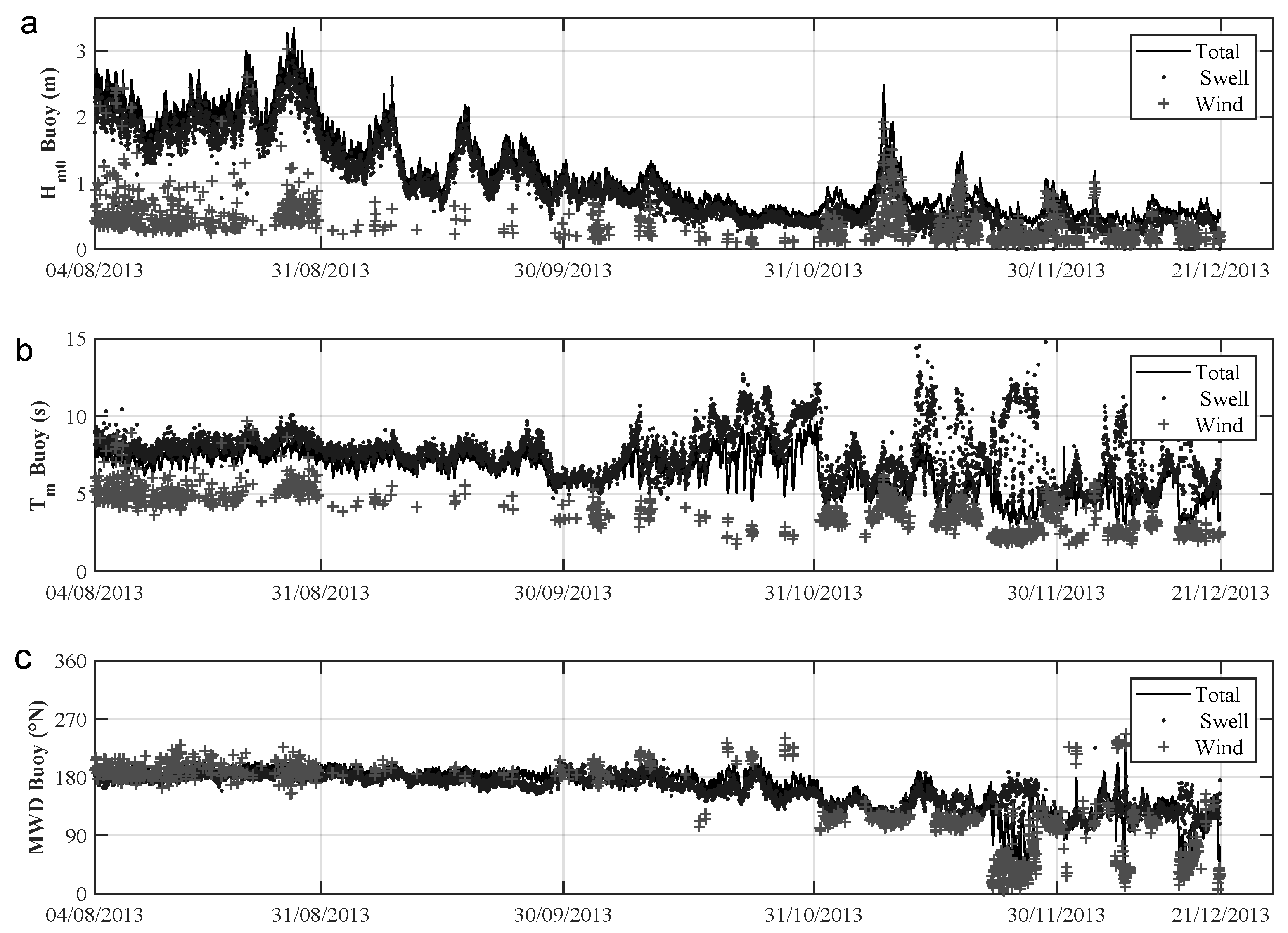
Swell and wind waves time series highlight during the monsoon season the presence of a steady swell wave field coming from SSW over which wind waves with almost the same direction superimpose (Figure 8). In the post-monsoon, storm events generated from NE monsoon wind can be easily detected.
Long-period swells with low wave heights (less than 1 m) and peak wave periods greater than 14 s have been observed in the post monsoon period (2.7% of the observed waves). When long waves occur, wave spectra typically present two different swell systems: a primary swell peak at 0.06 Hz and a secondary swell peak at 0.1 Hz. Long waves along the eastern Arabian Sea are typical of pre and post-monsoon periods, while during the SW monsoon their occurrence frequency is low due to the strong winds that affect the Indian Ocean [57,58].
3.4. Comparison between Observed Data and ERA Wave Datasets
As a preliminary step, observed wave data have been compared to ERA5 and ERA-I wave datasets in order to evaluate the wave model performance in that region. Since no comparison had ever been carried out on the ERA-I data offshore Oman, it seemed useful to investigate those data, even if they are outdated and ERA5 is the latest global wave model. The comparison has been carried out using a back-propagation approach in which waves recorded by the buoy near the coast are refracted back to the nearest ERA grid node (located about 50 km offshore the Oman coast). The wave height in the nearest ERA grid point has been estimated from the observed wave height by using the energy flux conservation principle, and considering simple, straight and parallel contours of the bathymetric configuration. The wave height at ERA point (suffix “M”) can be estimated from buoy observation point (suffix “B”) as
where H is the significant wave height, is the wave direction and is the group velocity.
A statistical comparison of observations and forecasts using ERA5 and ERA-I wave models highlights that the ERA5 wave model has a better performance for wave heights estimation (Figure 9). Mean error, standard deviation and root mean square error (RMSE), relative bias and coefficient of determination () have been estimated for the numerical datasets, and results have shown an RMSE of 0.23 m for ERA5, lower than RMSE estimated for ERA-I data (0.26 m).
Considering the best results of ERA5 wave model, further analyses on ERA5 wave data have been carried out, evaluating the model’s performance. Table 2 reports all the statistical parameters estimated in the monsoon and post-monsoon season. During the SW-monsoon period the model is rated as unsatisfactory (NSE = 0.515) with a wave height overestimation (RMSE = 0.32 m) and a quite low relative bias = 0.08 %). During the post-monsoon period, the fit results span from unsatisfactory to acceptable (NSE = 0.679), and simulated wave heights present a overestimation (RMSE = 0.19 m) and a higher relative bias (bias = 0.185%).
As proposed by [13] the ERA5 mean wave period (MWP) has been compared to the energy wave period (). MWP time series obtained from ERA5 dataset are rated unsatisfactory in the monsoon season (NSE = 0.178 and acceptable (NSE = 0.677) in the post-monsoon.
A rather good agreement can be seen between ERA5 MWD and observed MWD, even if during post-monsoon period ERA5 MWD are more easterly than measured MWD (as a negative bias is present).
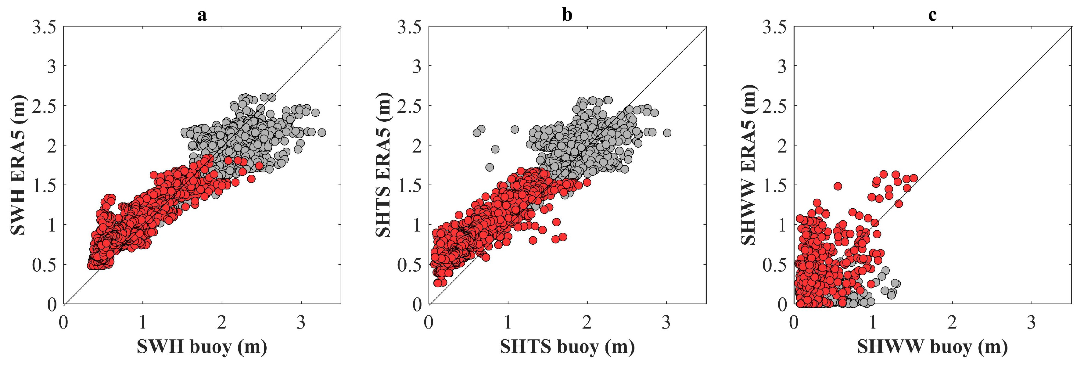
In order to explain such seasonal differences in wave model performance, further analyses have been performed, evaluating the model’s performance for swell and wind waves’ predictions separately. Figure 10 reports all the comparisons carried out: (a) a scatterplot of observed significant wave height of combined wind waves and swell versus ERA5 values; (b) a scatterplot of observed significant swell wave height versus ERA5 values; (c) a scatterplot of observed significant wind wave height versus ERA5 values. In all panels of Figure 10, red dots represent observed/predicted wave heights in the post monsoon season (October, November and December). The ERA5 wave dataset has two different performances in wave height prediction depending on wave type: swell wave height is generally overestimated both in monsoon and post-monsoon seasons, whereas wind wave height seems to be less accurate in the monsoon-season.
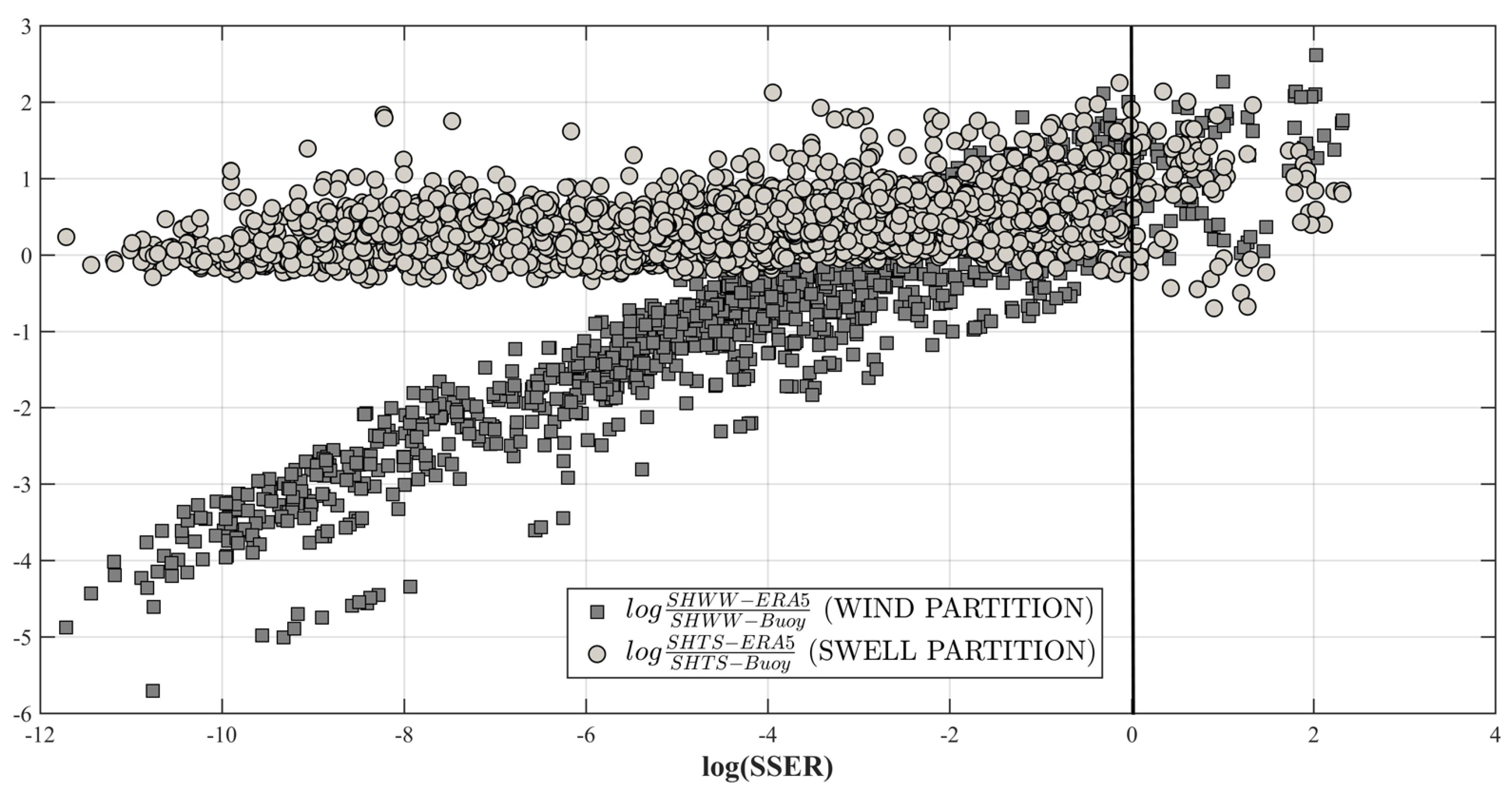
Moreover, the performance of the model was analyzed according to the value of wind wave–swell energy ratio SSER [59] (Figure 11). If SSER ≫ 1, the sea states are classified as wind waves. Waves are identified as swells if SSER≪ 1. For other cases a mixed sea state is present.
It can be easily observed that more than 80% of modeled sea states can be classified as swell and ERA5 SHTS are usually greater than observed swell heights in all sea state conditions (swell-dominated, wind wave-dominated and mixed sea states). In the case of swell-dominated states, ERA5 SHWW are underestimated, whereas in wind wave domination, conditions are usually overestimated. As also reported in Figure 9 the ERA5 wave model fails in prediction of wave heights particular likely when a persistent swell condition occurs as in the monsoon season.
4. Concluding Remarks
In order to identify the sea state conditions in which the numerical (wave) models get reliable results, a correct evaluation of the performances of numerical wave models first requires an accurate definition of the local framework in which they are applied.
The procedure outlined in this paper is intended to provide a general approach for wave field classification and wave model performance assessment in complex sea states when growing wind waves superimpose on a swell system.
The methodological approach has been applied to an observed wave dataset recorded in the Arabian Sea offshore southern Oman coast in the second half of 2013 during the monsoon and the post-monsoon seasons. The observed wave time series highlights a clear distinction between the SW monsoon and post-monsoon periods: in the first period the buoy recorded highest waves coming almost exclusively from the south, whereas in the following months waves were lower and coming from ESE and SSE. Significant variability in the monthly averaged spectrum has been observed: spectra are single peaked swells in August and September, whereas spectra are multipeaked with generated waves that coexist with the distant swells from the south Indian Ocean from October to December. In such wave conditions, it was found that the best possible results in wave spectra separation were provided by using a 2D spectral partition. Swell and wind wave systems can be detected only if a directional spectral analysis is carried out.
Once the recorded wave data have been analyzed and local sea wave climate has been defined, the observed data have been exploited to validate ERA5 wave model performance in the region. The results of the wave model validation highlighted that the wave model has two different performances depending on the sea condition. The model verification has been carried out for each season using a validation model that combines “good-of-fit parameters” and statistical significance instead of the widely-used coefficient of determination. The [52] validation model helps in overcoming problems in interpretation of NSE values, that can often be subjective, proposing four model performance classes. The analysis has shown that during the monsoon season the numerical dataset presents relevant issues in swell wave height and wave period reconstruction. During the post-monsoon period, the hindcast is also affected by biases and errors.
Furthermore, according to wind wave–swell energy ratio (SSER) the comparison has shown an overestimation in terms of swell wave heights for all sea-state conditions. A underestimation of wind wave heights in swell-dominating conditions is also observed. In wind wave dominated conditions, both swell and wind waves are overestimated.
The total significant wave height overestimation is probably due to swell wave height overestimation, as also reported for ERA-I wave dataset by [13] in the North Indian Ocean and [2] in swell-dominated basins. For the overall wave height overestimation, the highest waves seem to be underestimated in accordance with [1], who found an overestimation of the upper percentile wave heights forecasted in the ERA-I dataset. Some of the discrepancies in the wave data comparison may be related to the coarse resolution of the wind input and wave model grids, as suggested by [10], who highlighted the importance of local wind influence and bathymetry effects in ERA-I wave model.
The ERA5 global model provides wave hindcast in a low-resolution grid, and a complex environment such as the nearshore Arabic Sea probably cannot be fully modeled. Thus, the ERA5 wave dataset allows one to describe wave and wind fields across the Arabian Sea, providing a regional overview and overcoming the lack of in situ data, but a finer nested grid model has to be implemented to predict wave field in that region. This is an ongoing activity.
Author Contributions
Conceptualization, M.F.B., M.G.M., V.T. and M.M.; data curation, M.F.B., M.G.M. and V.T.; formal analysis, M.F.B., M.G.M. and V.T.; funding acquisition, M.M.; investigation, M.F.B., M.G.M. and V.T.; methodology, M.F.B., M.G.M., V.T. and M.M.; resources, M.F.B. and M.G.M.; software, M.F.B., M.G.M. and V.T.; supervision, M.M.; validation, M.F.B., M.G.M. and V.T.; visualization, M.F.B., M.G.M. and V.T.; writing—original draft, M.F.B. and M.G.M; writing—review and editing, M.F.B., M.G.M., V.T. and M.M. All authors have read and agreed to the published version of the manuscript.
Funding
This research received no external funding.
Acknowledgments
The authors thank Francesco De Giosa for providing raw data and for the fruitful collaboration. The authors thank VM Aboobacker for valuable comments and suggestions that greatly improved the interpretation of the data.
Conflicts of Interest
The authors declare no conflict of interest.
Appendix A. List of Wave and “Goodness-of-Fit” Parameters
- moment of energy spectrum
- Significant wave height
- Mean wave period
- Mean zero-crossing period
- Energy period
- Mean wave direction
- Directional Spread of
- Significant wave steepness
- Peakedness parameter
- Spectral width parameter
- Narrowness parameter
- Root mean squared error
- Relative bias
- Coefficient of determination
- Coefficient of efficiency
- Circular correlation coefficient
References
- Stopa, J.E.; Cheung, K.F. Intercomparison of wind and wave data from the ECMWF Reanalysis Interim and the NCEP Climate Forecast System Reanalysis. Ocean Model. 2014, 75, 65–83. [Google Scholar] [CrossRef]
- Aarnes, O.J.; Abdalla, S.; Bidlot, J.R.; Breivik, Ø. Marine wind and wave height trends at different ERA-Interim forecast ranges. J. Clim. 2015, 28, 819–837. [Google Scholar] [CrossRef] [Green Version]
- Pasquali, D.; Bruno, M.; Celli, D.; Damiani, L.; Di Risio, M. A simplified hindcast method for the estimation of extreme storm surge events in semi-enclosed basins. Appl. Ocean Res. 2019, 85, 45–52. [Google Scholar] [CrossRef]
- Nitti, D.O.; Nutricato, R.; Lorusso, R.; Lombardi, N.; Bovenga, F.; Bruno, M.F.; Chiaradia, M.T.; Milillo, G. On the geolocation accuracy of COSMO-SkyMed products. In SAR Image Analysis, Modeling, and Techniques XV; International Society for Optics and Photonics, SPIE: Washington, DC, USA, 2015; Volume 9642, pp. 69–80. [Google Scholar]
- Bruno, M.F.; Molfetta, M.G.; Pratola, L.; Mossa, M.; Nutricato, R.; Morea, A.; Nitti, D.O.; Chiaradia, M.T. A combined approach of field data and earth observation for coastal risk assessment. Sensors 2019, 19, 1399. [Google Scholar] [CrossRef] [Green Version]
- Di Risio, M.; Bruschi, A.; Lisi, I.; Pesarino, V.; Pasquali, D. Comparative Analysis of Coastal Flooding Vulnerability and Hazard Assessment at National Scale. J. Mar. Sci. Eng. 2017, 5, 51. [Google Scholar] [CrossRef] [Green Version]
- Sterl, A.; Caires, S. Climatology, variability and extrema of ocean waves: The Web-based KNMI/ERA-40 wave atlas. Int. J. Climatol. 2005, 25, 963–977. [Google Scholar] [CrossRef]
- Semedo, A.; Sušelj, K.; Rutgersson, A.; Sterl, A. A global view on the wind sea and swell climate and variability from ERA-40. J. Clim. 2011, 24, 1461–1479. [Google Scholar] [CrossRef]
- Zhang, J.; Wang, W.; Guan, C. Analysis of the global swell distributions using ECMWF Re-analyses wind wave data. J. Ocean Univ. China (Engl. Ed.) 2011, 10, 325–330. [Google Scholar] [CrossRef]
- Ardhuin, F.; Bertotti, L.; Bidlot, J.R.; Cavaleri, L.; Filipetto, V.; Lefevre, J.M.; Wittmann, P. Comparison of wind and wave measurements and models in the Western Mediterranean Sea. Ocean Eng. 2007, 34, 526–541. [Google Scholar] [CrossRef]
- Cavaleri, L. The wind and wave atlas of the Mediterranean Sea-the calibration phase. Adv. Geosci. 2005, 2, 255–257. [Google Scholar] [CrossRef] [Green Version]
- Cavaleri, L.; Sclavo, M. The calibration of wind and wave model data in the Mediterranean Sea. Coast. Eng. 2006, 53, 613–627. [Google Scholar] [CrossRef]
- Kumar, V.S.; Naseef, M. Performance of ERA-Interim wave data in the nearshore waters around India. J. Atmos. Oceans Technol. 2015, 32, 1257–1269. [Google Scholar] [CrossRef]
- Deo, M.C.; Jha, A.; Chaphekar, A.S.; Ravikant, K. Neural networks for wave forecasting. Ocean Eng. 2001, 28, 889–898. [Google Scholar] [CrossRef]
- Zamani, A.; Solomatine, D.; Azimian, A.; Heemink, A. Learning from data for wind–wave forecasting. Ocean Eng. 2008, 35, 953–962. [Google Scholar] [CrossRef]
- De Girolamo, P.; Di Risio, M.; Beltrami, G.; Bellotti, G.; Pasquali, D. The use of wave forecasts for maritime activities safety assessment. Appl. Ocean Res. 2017, 62, 18–26. [Google Scholar] [CrossRef]
- Chen, G.; Chapron, B.; Ezraty, R.; Vandemark, D. A global view of swell and wind sea climate in the ocean by satellite altimeter and scatterometer. J. Atmos. Oceans Technol. 2002, 19, 1849–1859. [Google Scholar] [CrossRef]
- Gulev, S.K.; Grigorieva, V.; Sterl, A.; Woolf, D. Assessment of the reliability of wave observations from voluntary observing ships: Insights from the validation of a global wind wave climatology based on voluntary observing ship data. J. Geophys. Res. Oceans 2003, 108. [Google Scholar] [CrossRef] [Green Version]
- De Serio, F.; Mossa, M. Environmental monitoring in the Mar Grande basin (Ionian Sea, Southern Italy). Environ. Sci. Pollut. Res. 2016, 23, 12662–12674. [Google Scholar] [CrossRef]
- De Serio, F.; Mossa, M. Meteo and Hydrodynamic Measurements to Detect Physical Processes in Confined Shallow Seas. Sensors 2018, 18, 280. [Google Scholar] [CrossRef] [Green Version]
- Armenio, E.; De Serio, F.; Mossa, M. Analysis of data characterizing tide and current fluxes in coastal basins. Hydrol. Earth Syst. Sci. 2017, 21, 3441–3454. [Google Scholar] [CrossRef] [Green Version]
- Valentini, N.; Damiani, L.; Molfetta, M.G.; Saponieri, A. New coastal video-monitoring system achievement and development. Coast. Eng. Proc. 2017, 1, 11. [Google Scholar] [CrossRef]
- Hersbach, H. News from C3S: ERA5. Presented at the Using ECMWF Forecast, Reading, UK, 12–16 June 2017. [Google Scholar]
- Ranjha, R.; Tjernström, M.; Semedo, A.; Svensson, G.; Cardoso, R.M. Structure and variability of the Oman coastal low-level jet. Tellus A Dyn. Meteorol. Oceanogr. 2015, 67, 25285. [Google Scholar] [CrossRef]
- Aboobacker, V.; Vethamony, P.; Rashmi, R. “Shamal” swells in the Arabian Sea and their influence along the west coast of India. Geophys. Res. Lett. 2011, 38. [Google Scholar] [CrossRef] [Green Version]
- Carr, C.M.; Yavary, M.; Yavary, M. Wave agitation studies for port expansion-Salalah, Oman. In Proceedings of the Ports 2004: Port Development in the Changing World, Houston, TX, USA, 23–26 May 2004; pp. 1–10. [Google Scholar]
- Goring, D. Ship surging induced by long waves in Port of Salalah, Oman. In Proceedings of the Coasts & Ports 2005 Conference, Adelaide, Australia, 20–23 September 2005; Volume 2023. [Google Scholar]
- Anoop, T.R.; Kumar, V.S.; Shanas, P.R.; Johnson, G. Surface Wave Climatology and Its Variability in the North Indian Ocean Based on ERA-Interim Reanalysis. J. Atmos. Oceans Technol. 2015, 32, 1372–1385. [Google Scholar] [CrossRef] [Green Version]
- Kumar, V.S.; Shanas, P.; Dubhashi, K. Shallow water wave spectral characteristics along the eastern Arabian Sea. Nat. Hazards 2014, 70, 377–394. [Google Scholar] [CrossRef]
- Kumar, V.S.; Nair, M.A. Inter-annual variations in wave spectral characteristics at a location off the central west coast of India. Ann. Geophys. 2015, 33, 159–167. [Google Scholar] [CrossRef]
- Rashmi, R.; Aboobacker, V.; Vethamony, P.; John, M. Co-existence of wind seas and swells along the west coast of India during non-monsoon season. Ocean Sci. 2013, 9, 281. [Google Scholar] [CrossRef] [Green Version]
- Vethamony, P.; Aboobacker, V.; Menon, H.; Kumar, K.A.; Cavaleri, L. Superimposition of wind seas on pre-existing swells off Goa coast. J. Mar. Syst. 2011, 87, 47–54. [Google Scholar] [CrossRef] [Green Version]
- Komen, G.J.; Cavaleri, L.; Donelan, M. Dynamics and Modelling of Ocean Waves; Cambridge University Press: Cambridge, UK, 1996. [Google Scholar]
- Hersbach, H.; de Rosnay, P.; Bell, B.; Schepers, D.; Simmons, A.; Soci, C.; Abdalla, S.; Alonso-Balmaseda, M.; Balsamo, G.; Bechtold, P.; et al. Operational Global Reanalysis: Progress, Future Directions and Synergies with NWP, ERA Report Series; ECMWF Shinfield Park: Reading, UK, 2018. [Google Scholar]
- Dee, D.P.; Uppala, S.; Simmons, A.; Berrisford, P.; Poli, P.; Kobayashi, S.; Andrae, U.; Balmaseda, M.; Balsamo, G.; Bauer, P.; et al. The ERA-Interim reanalysis: Configuration and performance of the data assimilation system. Q. J. R. Meteorol. Soc. 2011, 137, 553–597. [Google Scholar] [CrossRef]
- Krogstad, H.E. Maximum likelihood estimation of ocean wave spectra from general arrays of wave gauges. Model. Identif. Control 1988, 9, 81–97. [Google Scholar] [CrossRef] [Green Version]
- Kuik, A.; Van Vledder, G.P.; Holthuijsen, L. A method for the routine analysis of pitch-and-roll buoy wave data. J. Phys. Oceanogr. 1988, 18, 1020–1034. [Google Scholar] [CrossRef]
- Longuet-Higgins, M. On the joint distribution of the periods and amplitudes of sea waves. J. Geophys. Res. 1975, 80, 2688–2694. [Google Scholar] [CrossRef]
- Longuet-Higgins, M.S. The statistical analysis of a random, moving surface. Philos. Trans. R. Soc. Lond. A Math. Phys. Eng. Sci. 1957, 249, 321–387. [Google Scholar]
- Cartwright, D.; Longuet-Higgins, M.S. The statistical distribution of the maxima of a random function. In Proceedings of the Royal Society of London A: Mathematical, Physical and Engineering Sciences; The Royal Society: London, UK, 1956; Volume 237, pp. 212–232. [Google Scholar]
- Goda, Y. Numerical experiments on wave statistics with spectral simulation. Rept. Port Harb. Res. Inst. 1970, 9, 3–57. [Google Scholar]
- Rye, H. Wave group formation among storm waves. In Proceedings of the 14th Conference on Coastal Engineering, Copenhagen, Denmark, 24–28 June 1974; pp. 164–183. [Google Scholar]
- Thompson, W.C.; Nelson, A.R.; Sedivy, D.G. Wave group anatomy of ocean wave spectra. In Proceedings of the 19th Conference on Coastal Engineering, Houston, TX, USA, 3–7 September 1984; pp. 661–677. [Google Scholar]
- Li, S.; Zhao, D. Comparison of spectral partitioning techniques for wind wave and swell. Mar. Sci. Bull. 2012, 14, 24–36. [Google Scholar]
- Portilla, J.; Ocampo-Torres, F.J.; Monbaliu, J. Spectral partitioning and identification of wind sea and swell. J. Atmos. Oceans Technol. 2009, 26, 107–122. [Google Scholar] [CrossRef]
- Chen, Z.; Zhang, L.; Zhao, C.; Chen, X.; Zhong, J. A Practical Method of Extracting Wind Sea and Swell from Directional Wave Spectrum. J. Atmos. Oceans Technol. 2015, 32, 2147–2159. [Google Scholar] [CrossRef]
- Pierson, W.J., Jr.; Moskowitz, L. A proposed spectral form for fully developed wind seas based on the similarity theory of SA Kitaigorodskii. J. Geophys. Res. 1964, 69, 5181–5190. [Google Scholar] [CrossRef]
- Alves, J.H.G.; Banner, M.L.; Young, I.R. Revisiting the Pierson–Moskowitz asymptotic limits for fully developed wind waves. J. Phys. Oceanogr. 2003, 33, 1301–1323. [Google Scholar] [CrossRef]
- Hanson, J.L.; Phillips, O.M. Automated analysis of ocean surface directional wave spectra. J. Atmos. Oceans Technol. 2001, 18, 277–293. [Google Scholar] [CrossRef]
- Hwang, P.A.; Ocampo-Torres, F.J.; García-Nava, H. Wind sea and swell separation of 1D wave spectrum by a spectrum integration method. J. Atmos. Oceans Technol. 2012, 29, 116–128. [Google Scholar] [CrossRef]
- Wang, D.W.; Hwang, P.A. An operational method for separating wind sea and swell from ocean wave spectra. J. Atmos. Oceans Technol. 2001, 18, 2052–2062. [Google Scholar] [CrossRef]
- Ritter, A.; Muñoz-Carpena, R. Performance evaluation of hydrological models: Statistical significance for reducing subjectivity in goodness-of-fit assessments. J. Hydrol. 2013, 480, 33–45. [Google Scholar] [CrossRef]
- Legates, D.R.; McCabe, G.J. Evaluating the use of “goodness-of-fit” measures in hydrologic and hydroclimatic model validation. Water Resour. Res. 1999, 35, 233–241. [Google Scholar] [CrossRef]
- Biondi, D.; Freni, G.; Iacobellis, V.; Mascaro, G.; Montanari, A. Validation of hydrological models: Conceptual basis, methodological approaches and a proposal for a code of practice. Phys. Chem. Earth Parts A/B/C 2012, 42, 70–76. [Google Scholar] [CrossRef]
- Jammalamadaka, S.R.; Sengupta, A. Topics in Circular Statistics; World Scientific: Singapore, 2001; Volume 5. [Google Scholar]
- Pai, D.; Bhan, S. Monsoon 2013—A Report; India Meteorological Department: Pune, India, 2014; pp. 1–222.
- Glejin, J.; Sanil Kumar, V.; Nair, B.; Singh, J. Influence of winds on temporally varying short and long period gravity waves in the near shore regions of the eastern Arabian Sea. Ocean Sci. 2013, 9, 343–353. [Google Scholar] [CrossRef] [Green Version]
- Glejin, J.; Kumar, V.S.; Amrutha, M.; Singh, J. Characteristics of long-period swells measured in the near shore regions of eastern Arabian Sea. Int. J. Nav. Archit. Ocean Eng. 2016, 8, 312–319. [Google Scholar] [CrossRef] [Green Version]
- Rodriguez, G.; Soares, C.G. The bivariate distribution of wave heights and periods in mixed sea states. J. Offshore Mech. Arct. Eng. 1999, 121, 102–108. [Google Scholar] [CrossRef]
Figure 1.
Process flowchart from data acquisition to expected outcomes.

Figure 2.
Study area: wave buoy location and ERA5 wave model grid point.

Figure 3.
Time series plot of significant wave height (a), mean wave period (b), peak wave period (c), mean wave direction MWD (d) and directional spread (e) from August to December 2013.
Figure 3.
Time series plot of significant wave height (a), mean wave period (b), peak wave period (c), mean wave direction MWD (d) and directional spread (e) from August to December 2013.

Figure 4.
Monthly wave roses. Nautical convention for wave directions (i.e., the direction where the waves come from).
Figure 4.
Monthly wave roses. Nautical convention for wave directions (i.e., the direction where the waves come from).

Figure 5.
Time series plot of spectral narrowness parameter (a), spectral width parameter (b), spectral peakedness (c) and significant wave steepness (d).
Figure 5.
Time series plot of spectral narrowness parameter (a), spectral width parameter (b), spectral peakedness (c) and significant wave steepness (d).

Figure 6.
Temporal variability in the normalized spectral energy density during the observed period (computed from half-hourly data). Spectral energy values normalized with respect to peak energy density. Red dots are located at the peak frequency.
Figure 6.
Temporal variability in the normalized spectral energy density during the observed period (computed from half-hourly data). Spectral energy values normalized with respect to peak energy density. Red dots are located at the peak frequency.

Figure 7.
Monthly average wave directional spectra. Spectral energy values normalized with respect to peak energy density.
Figure 7.
Monthly average wave directional spectra. Spectral energy values normalized with respect to peak energy density.

Figure 8.
Time series plot of wave characteristics estimated from partitioned spectra: significant wave height, wind wave and swell height (a); mean wave period, wind wave and swell mean wave period (b); and mean wave direction, wind wave and swell mean wave direction (c).
Figure 8.
Time series plot of wave characteristics estimated from partitioned spectra: significant wave height, wind wave and swell height (a); mean wave period, wind wave and swell mean wave period (b); and mean wave direction, wind wave and swell mean wave direction (c).

Figure 9.
Comparison of the synchronous wave heights extracted from ERA wave models against the back-propagated observed wave heights at the nearest ERA5 grid node.
Figure 9.
Comparison of the synchronous wave heights extracted from ERA wave models against the back-propagated observed wave heights at the nearest ERA5 grid node.

Figure 10.
Scatter plot of the synchronous wave heights extracted from ERA5 wave models against the back-propagated observed wave heights at the nearest ERA grid node: (a) observed SWH vs. ERA5 SWH; (b) observed SHTS vs. ERA5 SHTS; (c) observed SHWW vs. ERA5 SHWW. Red dots represent wave heights in the post-monsoon season (October, November and December).

Figure 11.
Scatter plot of wind waves-swell energy ratio SSER values against the ratio between the predicted and observed wave heights for wind (square markers) and swell partition (circle markers).
Figure 11.
Scatter plot of wind waves-swell energy ratio SSER values against the ratio between the predicted and observed wave heights for wind (square markers) and swell partition (circle markers).


Table 1.
Seasonal variability of wave characteristics observed in offshore Salalah.
| Parameter | AUG-SEP | OCT-NOV-DEC | ||
|---|---|---|---|---|
| Average | Range | Average | Range | |
| (m) | 2.85 | 1.02–5.94 | 1.13 | 0.30–4.01 |
| (m) | 1.08 | 0.42–2.04 | 0.42 | 0.10–1.50 |
| (m) | 1.21 | 0.46–2.28 | 0.47 | 0.21–1.67 |
| (m) | 1.70 | 0.64–3.22 | 0.66 | 0.29–2.32 |
| (m) | 2.11 | 0.80–3.99 | 0.82 | 0.25–2.96 |
| (s) | 6.81 | 4.97–8.42 | 5.34 | 2.90–9.69 |
| (s) | 8.32 | 5.98–9.87 | 7.14 | 3.23–12.11 |
| (s) | 8.39 | 6.05–10.3 | 7.75 | 3.24–13.74 |
Table 2.
Seasonal variability of goodness-of-fit metrics used for comparison of the ERA5 data with the observed wave data.
Table 2.
Seasonal variability of goodness-of-fit metrics used for comparison of the ERA5 data with the observed wave data.
| AUG-SEP | OCT-NOV-DEC | ||
|---|---|---|---|
| RMSE (m) | 0.32 | 0.19 | |
| Relative Bias (%) | 0.08 | 0.185 | |
| 0.60 | 0.81 | ||
| NSE | 0.515 | 0.679 | |
| RMSE (m) | 0.431 | 0.770 | |
| Relative Bias (%) | −0.02 | −0.05 | |
| 0.36 | 0.72 | ||
| NSE | 0.178 | 0.667 | |
| MWD | RMSE (deg) | 10.29 | 27.29 |
| Bias (deg) | −7.675 | −20.25 | |
| −0.02 | 0.909 |
© 2020 by the authors. Licensee MDPI, Basel, Switzerland. This article is an open access article distributed under the terms and conditions of the Creative Commons Attribution (CC BY) license (http://creativecommons.org/licenses/by/4.0/).
Share and Cite
MDPI and ACS Style
Bruno, M.F.; Molfetta, M.G.; Totaro, V.; Mossa, M. Performance Assessment of ERA5 Wave Data in a Swell Dominated Region. J. Mar. Sci. Eng. 2020, 8, 214. https://doi.org/10.3390/jmse8030214
AMA Style
Bruno MF, Molfetta MG, Totaro V, Mossa M. Performance Assessment of ERA5 Wave Data in a Swell Dominated Region. Journal of Marine Science and Engineering. 2020; 8(3):214. https://doi.org/10.3390/jmse8030214
Chicago/Turabian StyleBruno, Maria Francesca, Matteo Gianluca Molfetta, Vincenzo Totaro, and Michele Mossa. 2020. "Performance Assessment of ERA5 Wave Data in a Swell Dominated Region" Journal of Marine Science and Engineering 8, no. 3: 214. https://doi.org/10.3390/jmse8030214
Note that from the first issue of 2016, this journal uses article numbers instead of page numbers. See further details here.