Comparison of HF Radar Fields of Directional Wave Spectra Against In Situ Measurements at Multiple Locations


1
Morphodynamique Continentale et Côtière, CNRS UMR 6143, Caen University, 14000 Caen, France
2
Coastal Processes Research Group, School of Biological and Marine Sciences, Plymouth University, Plymouth PL4 8AA, UK
*
Author to whom correspondence should be addressed.
J. Mar. Sci. Eng. 2019, 7(8), 271; https://doi.org/10.3390/jmse7080271
Submission received: 19 June 2019
/
Revised: 7 August 2019
/
Accepted: 12 August 2019
/
Published: 14 August 2019
(This article belongs to the Special Issue Radar Technology for Coastal Areas and Open Sea Monitoring)
Abstract
:The coastal zone hosts a great number of activities that require knowledge of the spatial characteristics of the wave field, which in coastal seas can be highly heterogeneous. Information of this type can be obtained from HF radars, which offer attractive performance characteristics in terms of temporal and spatial resolution. This paper presents the validation of radar-derived fields of directional wave spectra. These were retrieved from measurements collected with an HF radar system specifically deployed for wave measurement, using an established inversion algorithm. Overall, the algorithm reported accurate estimates of directional spectra, whose main distinctive characteristic was that the spectral energy was typically spread over a slightly broader range of frequencies and directions than in their in situ-measured counterparts. Two errors commonly reported in previous studies, namely the overestimation of wave heights and noise related to short measurement periods, were not observed in our results. The maximum wave height recorded by two in situ devices differed by 30 cm on average from the radar-measured values, and with the exception of the wave spreading, the standard deviations of the radar wave parameters were between 3% and 20% of those obtained with the in situ datasets, indicating the two were similarly grouped around their means. At present, the main drawback of the method is the high quality signal required to perform the inversion. This is in part responsible for a reduced data return, which did not exceed 55% at any grid cell over the eight-month period studied here.
1. Introduction
Knowledge of the offshore and coastal wave climate is crucial for ensuring the successful outcome of several human activities such as marine operations, coastal defence, or marine energy extraction. Most of the projects associated to these activities require high quality data, with good temporal and spatial resolution, at several stages of their development. Among the tools able to retrieve spatial data, HF radar is a remote sensing technique that has the capability of providing a relatively large coverage with high temporal and spatial resolution. Nowadays, this technology plays an essential role in monitoring surface currents ([1,2,3]), whereas the suitability of its wave products for different applications has only recently begun to be explored ([4,5,6,7]).
The wave directional spectrum retrieved by HF radars is derived from backscattered signals reflected primarily off waves satisfying the Bragg resonance condition. Standard spectral techniques are then applied to transform these signals into Doppler spectra [8] that can be subsequently inverted into wave directional spectra ([9,10,11,12,13,14]), or some of its summary parameters ([15,16,17,18,19,20,21,22]).
The focus of this work is the inversion method presented in [23], which is distributed as a software package by Seaview Sensing Ltd., Sheffield, UK (Seaview hereafter). Its results have been previously examined using datasets collected during different experiments (e.g., [7,24,25,26]), which have revealed the accuracy and limitations of the method and the HF radar technique itself. Reported inaccuracies have been found to originate predominantly from two different sources: limitations in the theory describing the relation between Doppler and ocean wave spectra [27], and the use of short averaging periods to derive wave directional spectra [28]. The main consequence of the former is an overestimation of high sea states ([24,25]), while the latter has been identified as the cause of noise in the measurements ([26,29,30]).
In this study, we used data collected with two operational phased-array Wellen Radars (WERA) to validate the Seaview algorithm. Results obtained with this method were derived from backscattered time series integrated over periods similar to those used by the in situ devices (17 min). With this approach, we intended to diminish the effect of short averaging on the results, to be able to clearly identify the contributions of other limitations as well as the ranges for which reliable data can be obtained.
The next section provides an overview of the study area and the devices that collected the data used here. This is followed by the intercomparison of radar and in situ wave integrated parameters and directional spectra, in Section 3. Finally, we provide a discussion of the results in Section 4, and the main conclusions derived from them are summarised in Section 5.
2. Materials and Methods
The measurements analysed in this work were collected over an area covering the Wave Hub; a grid connected wave energy site for testing offshore renewable energy technologies located in the north coast of Cornwall (UK). In this region, the wave climate is a combination of the long period swell that propagates across the North Atlantic and locally generated wind waves, which are both modified by a current field that is largely dominated by tidal streams reaching 1 m s [31]. The area is well exposed to waves arriving from the west and southwest, and to some extent shielded by Ireland from waves coming from the northwest [31]. The prevailing wind directions are between south-southwest and northwest, with northeasterly winds increasing their frequency in late winter and spring. Winds of 8 m s or greater occur about half of the time in autumn and winter, and only 25% and 15% during spring and summer, respectively [32]. Typical wave conditions are represented by waves of 1.6 m significant wave height and 6 s mean period, while the conditions with one-year return period can reach the 10 m significant wave height and 12 s period [31].
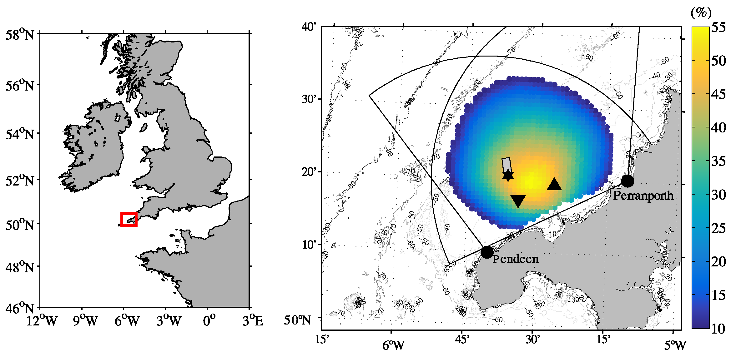
Two WERA radars were installed in 2011 to study the feasibility of using such devices to monitor wave conditions and provide useful data for Marine Renewable Energy (MRE) projects. The individual stations are located at Pendeen and Perranporth (Figure 1), approximately 40 km apart. Each site consists of a 16-element phased-array receiver and a 4-element transmitter. Independent measurements are synchronously acquired at the two stations for 17 min 45 s, every hour, at approximately 600 m range resolution and angular resolution. The two radars operate around a center frequency of 12.3 MHz in a “listen-before-talk” mode [33], determining the cleanest frequency band within 250-kHz. At the center transmitting frequency, the backscatter is dominated by Bragg reflection off 12.5 m waves, and the theoretically measurable sea states range from wave heights between 0.4 and 8 m, and have an upper frequency limit of approximately 0.28 Hz, although the latter will change depending on the intersection angle between wind and radar beam. These limits are dictated by the theory behind the Seaview method, and the reader is referred to [27] for more information about them. Finally, with this configuration, the maximum range for wave measurements is about 50 km.
2.1. Datasets
2.1.1. HF Radar
The dataset used in this study, chosen to coincide with a period when in situ measurements were available, was collected between April and November 2012. During this period, the two radars were simultaneously operational 98% of the time, while the maximum wave data return of the inversion algorithm at any one cell within the radar coverage was 55% (Figure 1). Low data return is generally associated with low signal-to-noise ratios (SNR), which are usually linked to low wind speeds. Under wind speeds between 0 and 4 m s, the data availability at the three cells where the in situ devices were deployed (see Figure 1) did not exceed 12%. Wind direction seems to also have an effect on data return, and the highest rate of success on the inversion is attained when the wind is blowing from the west (see Figure 2). In that situation, data were inverted 60% of the time, while this percentage decreased to about 40% when the wind was blowing from the three remaining fetch-limited quadrants.
Radar directional ocean wave spectra were computed from the recorded backscatter using the Seaview algorithm. The method is an iterative scheme initialized with a Pierson–Moskovitz spectrum and a cardioid model for the directional distribution, both of which are defined using information directly extracted from the radar-measured Doppler spectrum [23]. This initial guess of the ocean wave spectrum is then used to derive a Doppler spectrum by integration of the equation relating the two [34]. The integrated result is then compared to that measured, and if the spectra differ from each other, the initial estimate of the ocean wave spectrum is adjusted in the following iteration until a certain convergence criterion is met [23]. The above process is performed as long as the SNR of the second order Doppler spectrum is higher than 15 dB, and the amplitude of the local minima around the strongest Bragg peak is 3 dB below the latter. The result is a wave number directional spectrum calculated over 30 directions and a variable band of wave numbers that depends on factors such as the transmitting frequency, the intersection angle between the radar beams, and the wind direction [35]. The wave number spectra retrieved by the algorithm were subsequently converted into directional frequency spectra using the wave dispersion relation as follows:
where,
Frequency spectra were then obtained integrating the result of Equation (1) over the available range of directions. Finally, these spectra were interpolated to a 0.01 Hz resolution over the frequency range 0.05–0.25 Hz.
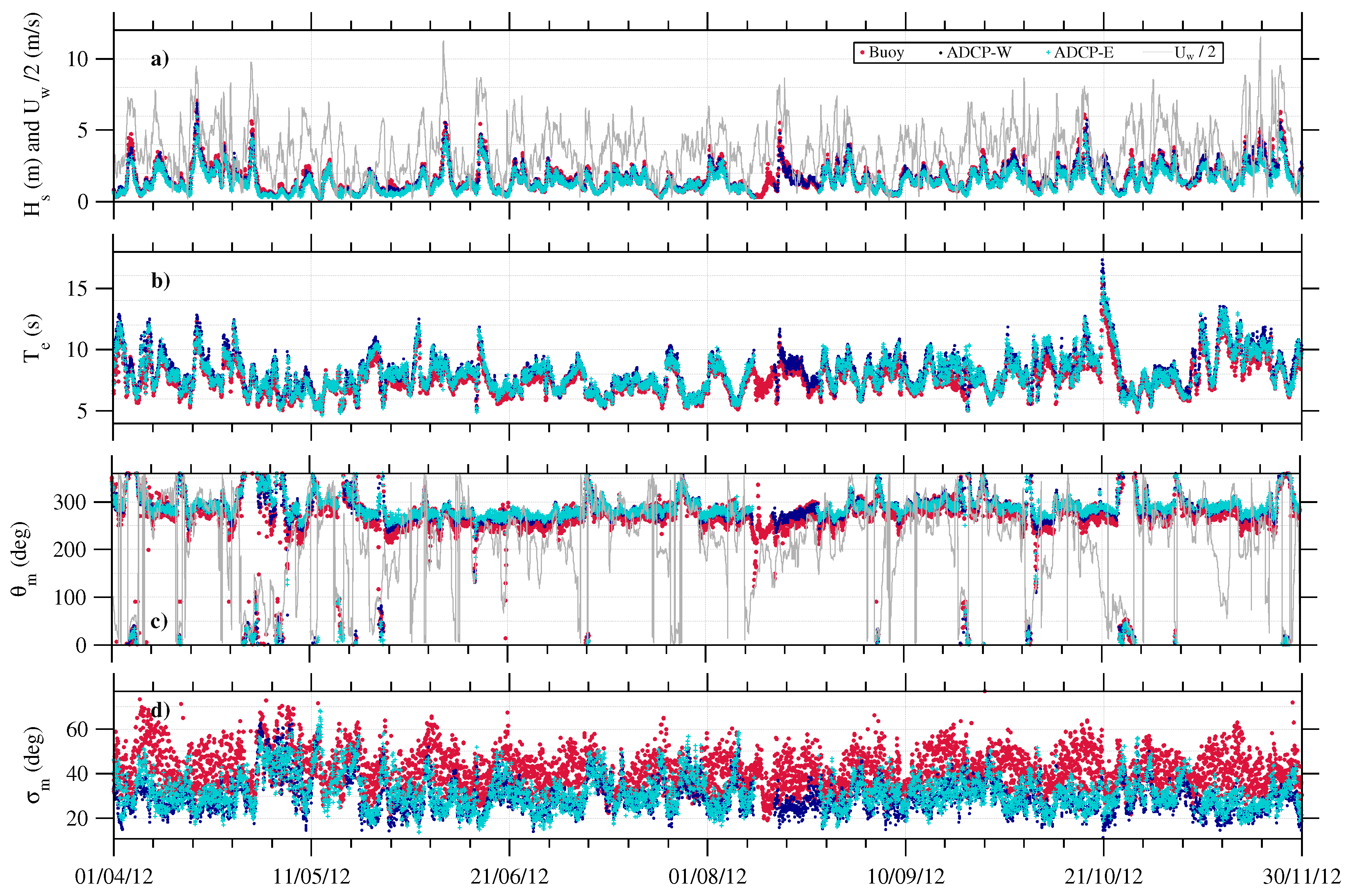
Wave parameters were then obtained from the frequency spectra and the first two directional Fourier coefficients. The time series derived from the radar and in situ measurements are shown in Figure 2 and Figure 3, respectively. The calculations were performed for the whole frequency range (0.05–0.25 Hz) and three additional sub-ranges; 4–6 s, 6–10 s, and 10–20 s as follows,
where is calculated from the first two Fourier coefficients as,
where is the frequency dependent directional spreading, calculated as,
In all equations, S(f) is the frequency spectrum, while and represent the lower and upper integration limits. The coefficients and are the first two Fourier coefficients calculated from the directional distribution [36].
2.1.2. Mooring Data
During 2012, two Acoustic Doppler Current Profilers (ADCPs) and a wave buoy were deployed in the area to provide data with which to validate the radar measurements against. From 13 March to 20 December 2012, a Seawatch Mini II directional wave buoy was deployed at 53 m depth, 20 km offshore from Pendeen and 30 km from Perranporth. The ADCPs, two upward looking 600-kHz Teledyne RDI WorkHorse Broadband, were deployed on the same day as the wave buoy, recovered on 16 May, and redeployed at the same locations on 18 May. Finally, after a second recovery on 11 August, the last deployment began three days later, on 14 August. The eastern-most ADCP, referred to as ADCP-E here, was located at 24 km from Pendeen and 19 km from Perranporth at a depth of 33 m, while the other (ADCP-W) was moored at 16 km from Pendeen and 29 km from Perranporth, at 35 m depth.
The ADCP orbital velocities were processed into directional spectra using RDI’s Wavesmon software. The iterative maximum likelihood method (IMLM [37]) was applied to compute directional spectra at 0.0078 Hz frequency resolution, and 36 directions at 15 resolution. In the processing, the effect of background currents was taken into account in order to avoid overestimation of wave heights due to the subsurface nature of the ADCP measurement [38]. The wave buoy time series were analyzed using WAFO [39]. Directional spectra were calculated using the extended maximum entropy method (EMEM [40]) at 128 frequency bins over 30 directions. Directional spectra were left unmodified, while the frequency spectra derived from them were interpolated to a 0.01 Hz frequency resolution and high- and low-pass filtered with cut-off frequencies of 0.05 and 0.25 Hz, respectively. Integrated parameters were then calculated using Equations (3)–(8). Further details about the devices and data processing can be found in [41].
2.2. Methodology
Common error metrics were used to evaluate the agreement between radar- and in situ-measured wave parameters. The root-mean-squared error (RMSE), the linear correlation (R) between two datasets, and the standard deviation of the data () were calculated as,
In Equations (9) and (10), x corresponds to the reference value and y is the radar measurement. The variables with an over-bar indicate mean values.
Whenever required, directional variables were compared using expressions from circular statistics. Mean values of the angular data were calculated by vector addition as described in [42],
where S and C are given by,
Then, the circular standard deviation can be calculated as,
where , with N the number of records. The RMSE for circular values was calculated as,
3. Results
3.1. Integrated Parameters
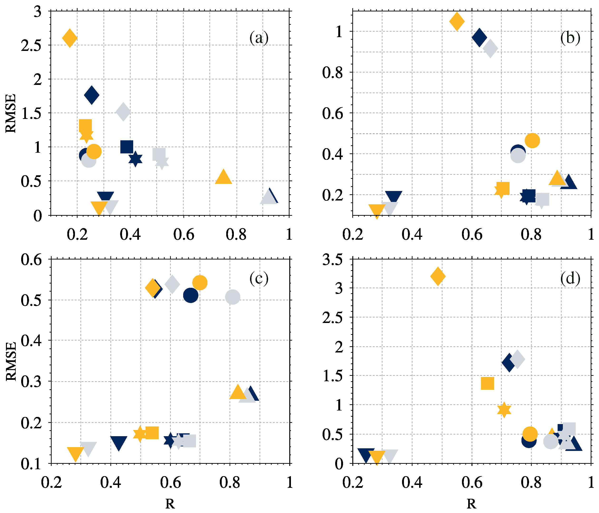
Figure 4 shows the values of RMSE and correlation derived from the comparison of the radar and in situ datasets. Results are shown for the frequency bands mentioned in the previous section (Figure 4a–c) and for the full range of available frequencies (Figure 4d).
Significant wave height is consistently well estimated across all frequency bands. Nonetheless, the performance of the algorithm for this parameter is optimal for 6.7–10 s period waves. Standard deviations (not shown) are close to those of the in situ devices for the energy containing waves (Figure 4b) and the full range of frequencies (Figure 4d), correlations (R) are above 0.8, and RMS differences are between 24 and 50 cm. The locally generated wind waves exhibit the lowest correlation to the in situ measurements (between 0.83 and 0.87), as well as a greater variability, represented by a standard deviation almost 1.5 times higher than the in situ values. Spatially, the poorest agreement appears on the ADCP-W comparisons. This device was deployed at the edge of Perranporth’s radar field of view, where the quality of the beamforming technique used by phased array radars to get azimuthal resolution and digitally steer the beam to the desired direction loses accuracy. In addition, the area is characterised by a slightly different surface current pattern than that of the rest of the radar’s field of view, with generally stronger current magnitudes. The combination of these two factors appears to result in wave spectra with spurious energy on their low frequencies.
The results for the energy and mean periods are very similar between them and show the same pattern seen for the significant wave height, with correlations around 0.9 and 0.8 for the bulk of the energy spectrum and waves between 6.7 and 10 s, respectively. The results degrade at the lowest frequency band, where the radar shows lower standard deviation than in situ measurements, correlations decrease to values between 0.25 and 0.5, and RMS errors are between 0.9 and 1.3 s.
Among the non-directional parameters, peak period is the least correlated to the in situ measurements. At the lowest frequency band, the results obtained for the buoy and ADCP-E comparisons show lower standard deviation than the in situ measurements, and correlations below 0.4. The agreement improves when comparing shorter swell and the bulk of the spectrum, both of which show similar results. Correlations in these cases are between 0.6 and 0.75, and radar standard deviations are equivalent to the wave buoy and lower than the ADCP-E. As found for the other parameters, the radar estimate at the ADCP-W site shows the poorest agreement to the in situ measurements at the lower frequency bands due to the peculiarities previously described, while the results for the short waves are very close to those obtained at the other two sites.
The agreement on the mean wave directions estimated by the radar and the in situ devices is generally satisfactory, and as already observed for the other parameters, the poorest performance was found at the low frequency band, where the results are marginally correlated to the in situ values, and RMS errors reach 27. In addition, the radar results show what it seems an unusual variability for this frequency band, which is represented by standard deviations two times higher than those of the ADCP results. The difference is smaller when comparing the results against the wave buoy, whose directions show higher variability than the ADCPs. Above 0.1 Hz, correlations increase to around 0.8, RMS errors lie between 11 and 19, and both radar and in situ devices show similar standard deviations.
Finally, with correlations below 0.5, the radar directional spread shows marginal agreement to the in situ measurements at all frequency bands. It is worth mentioning the opposite behavior of the radar’s standard deviation when compared to the wave buoy and the ADCPs, respectively. While the results show a higher variability on the radar’s wave spread when compared to the ADCPs, the result is reversed when the comparison is made against the wave buoy (Table 1).
3.2. Directional Wave Spectra
Direct comparison of directional spectra is not a straightforward task [43] and a qualitative analysis, based on the description of the graphical representation of the two types of results, is the common approach to this exercise. Here, we provide comparisons of three representative case studies.
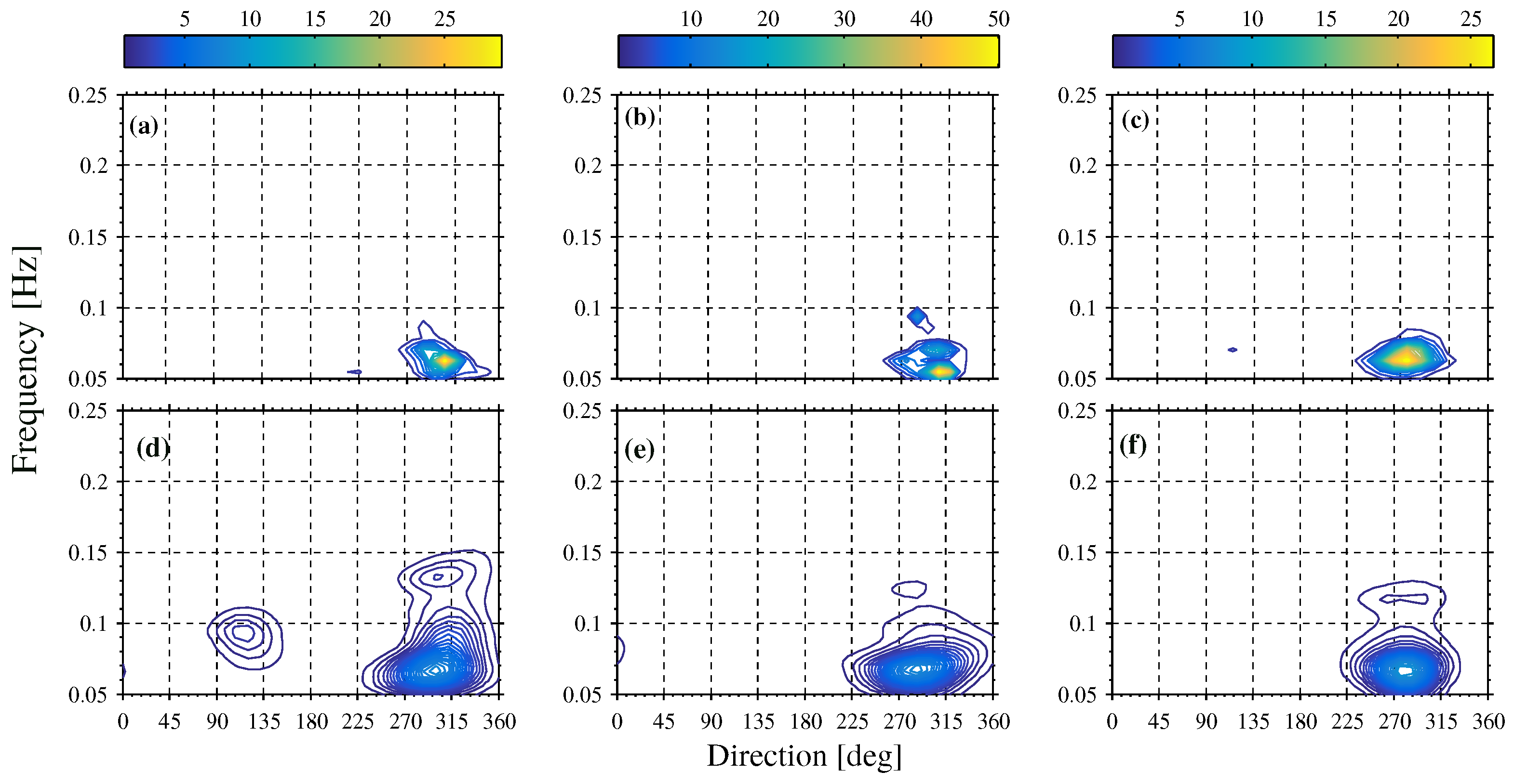
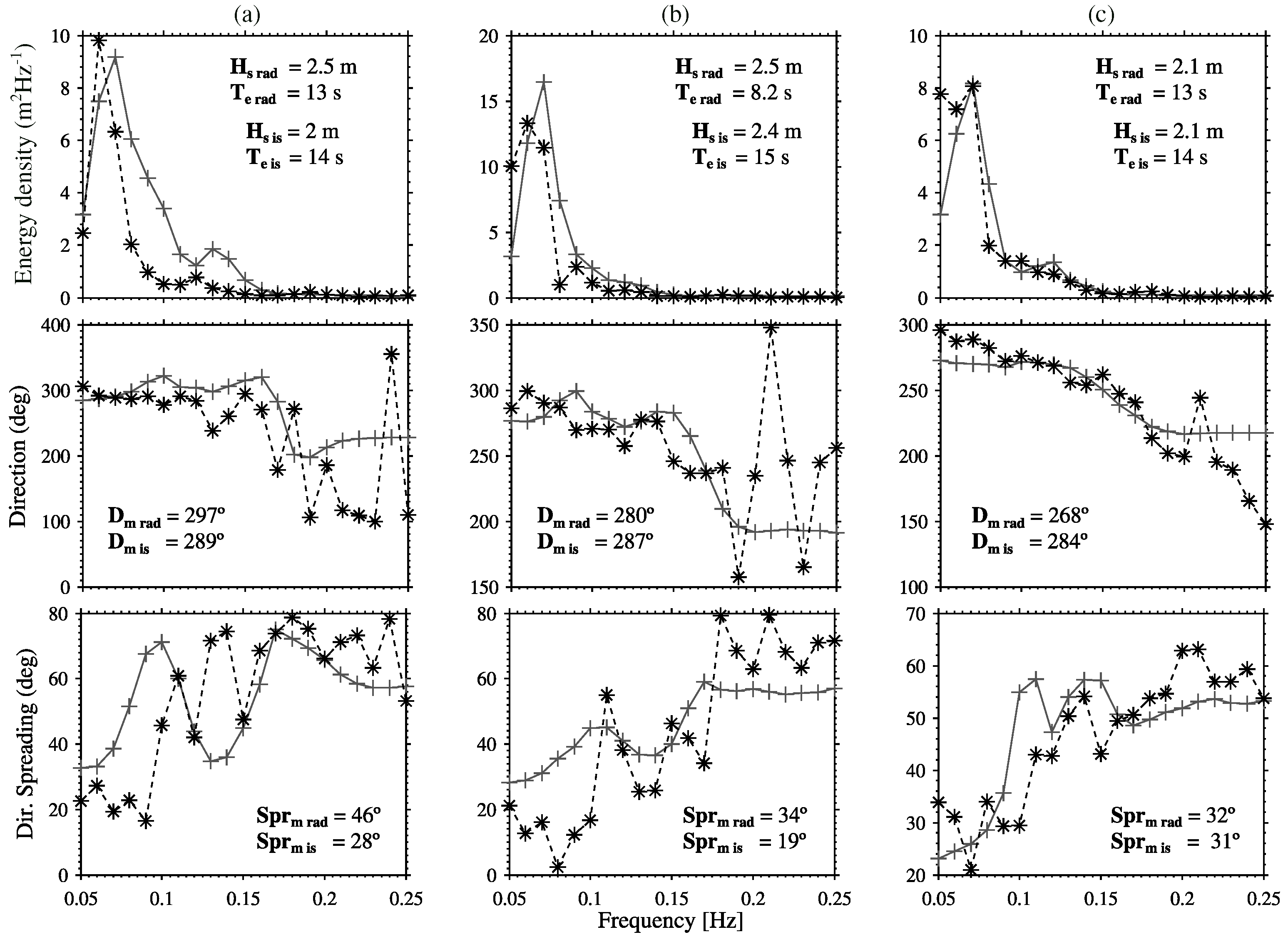
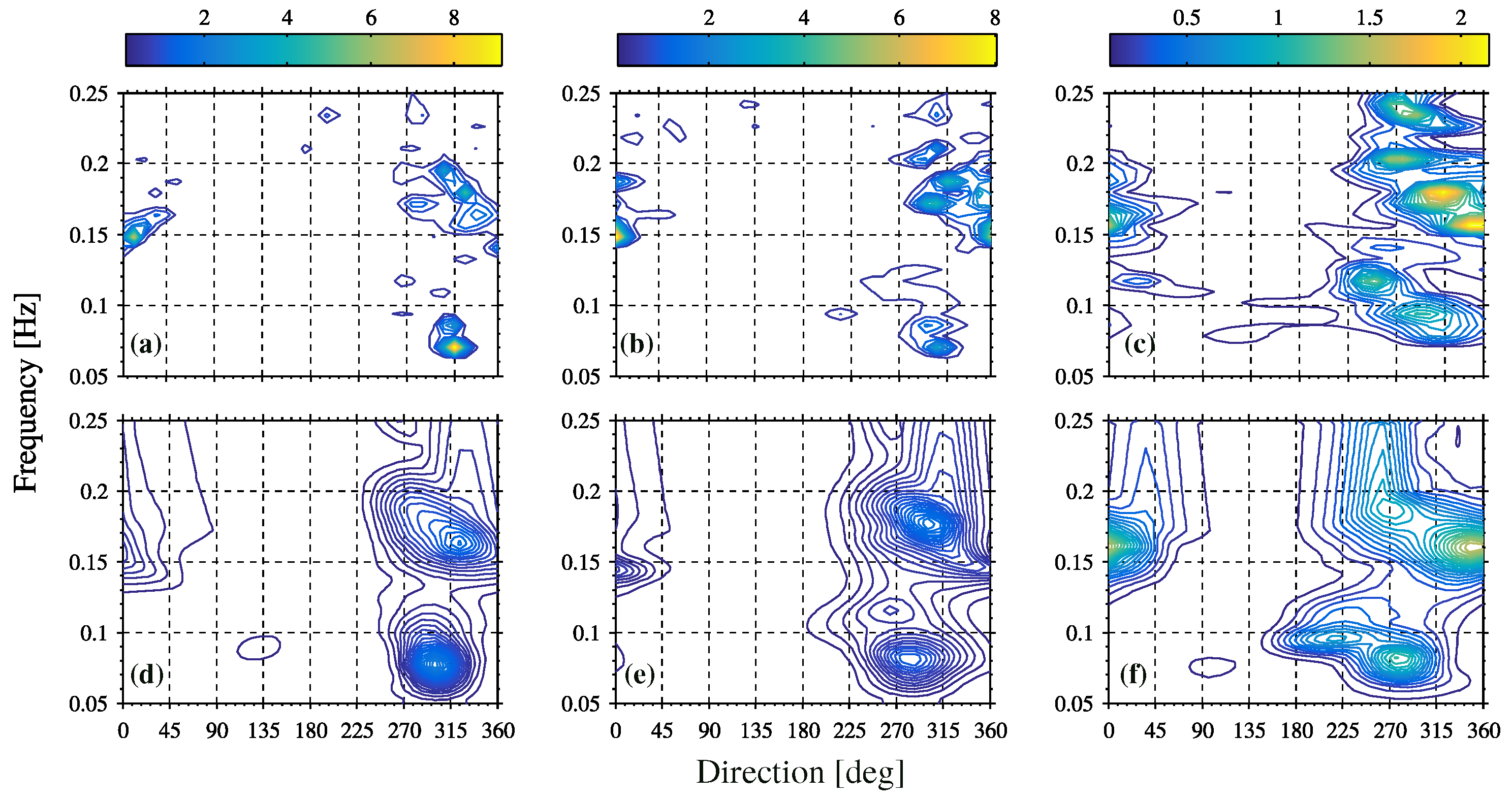
The longest swell recorded over the period analyzed here arrived to the study area on the first hours of 21 October. At 1000 UTC, a moderate wind was blowing from the east at 7 m s and the wave field was dominated by this long period swell, whose peak direction was determined to be about 280 10 by both radar and in situ devices. At the ADCP-E site (Figure 5a,d), the radar shows a secondary mode close to 0.1 Hz and 120 that was not observed by the in situ device. The same had been observed by the radar at the other two locations the previous two hours, and there is some energy on the buoy spectrum around the same direction, which seems to indicate that is not an error on the radar estimate.
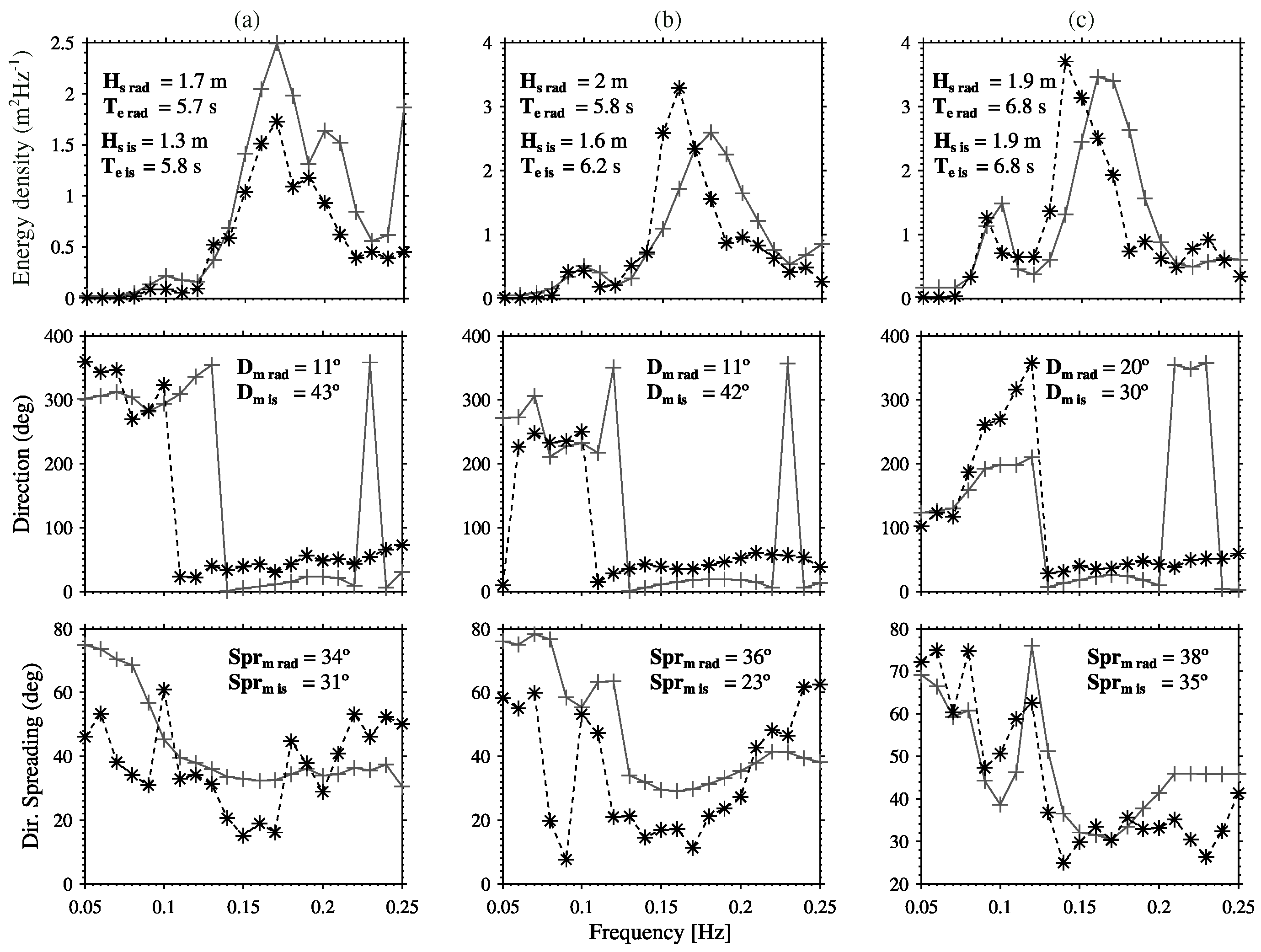
Figure 6 shows the integrated one-dimensional representations of spectral energy, direction and spread derived from the directional spectra of Figure 5. The spectra match very well across the three sites, and the biggest disagreement was observed on the ADCP-E comparison, which reveals a much broader radar spectrum, and a difference of 0.01 Hz on the estimated peak frequency that was also seen on the ADCP-W comparison. The directional spread measured by the different techniques shows what was seen on the previous section: radar measurements higher than the ADCPs over the low frequencies and slightly lower at the higher frequency end, and the opposite behavior on the radar-buoy comparison. Despite these differences, both radar and in situ devices show narrow distributions at the peak of the spectra, which broaden far from it.
On 24 September at 1100 UTC, the wave field was formed by a low frequency swell and a wind sea both very close in direction (Figure 7). On the afternoon of the day before, the wind speed had grown very rapidly from 5 to 11 m s while turning north from a more easterly direction. At the time of the observations described here, the wind had been steadily blowing for about 14 h and had a westerly direction. The radar-derived two-dimensional spectra show broader contours than the in situ spectra, especially when compared to the ADCPs, whose results are sharper than those of the buoy, possibly because the greater number of degrees of freedom in the measurements [44]. The swell measured by the radar at the buoy site exhibits two modes propagating from 220 and 280, and very close in frequency. Although the same is reported by the in situ device, the direction of arrival is about 10 further north and at slightly higher frequencies. The results of the wave directional spreading (Figure 8) show higher values on the low frequencies of the radar estimates as compared to the ADCPs, and lower above 0.19 Hz. This is reversed on the buoy comparison, where the radar spread is lower at the low frequency and higher above 0.16 Hz.
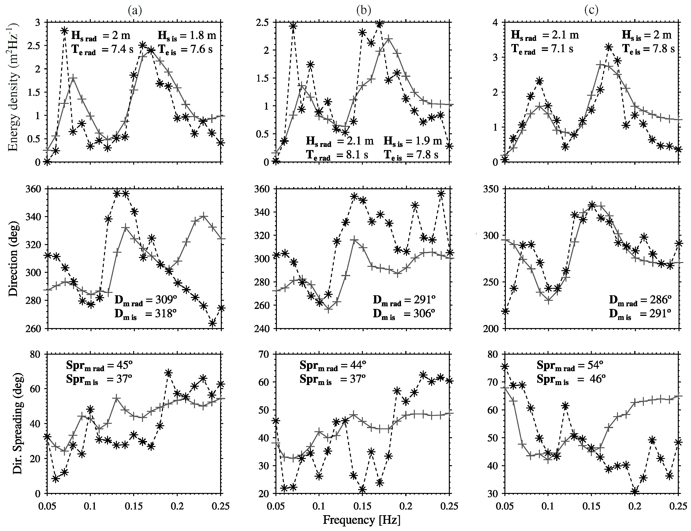
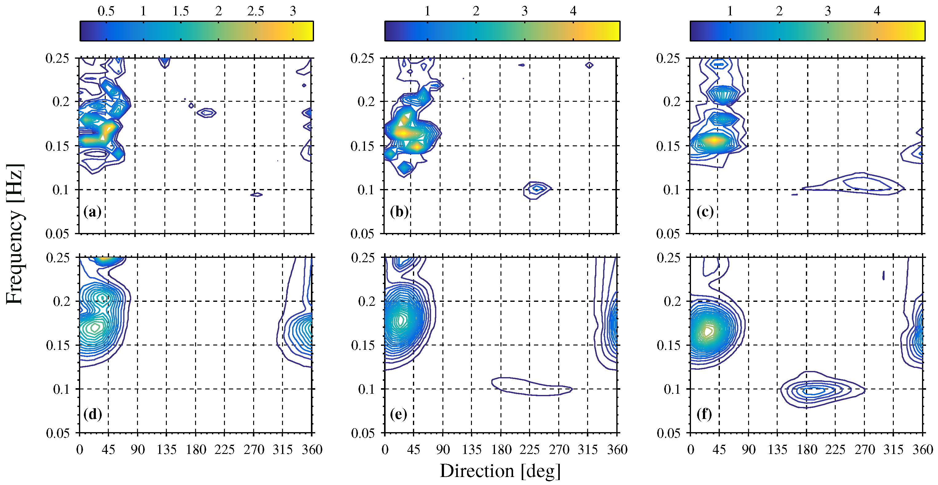
On 26 October at 0100 UTC, the directional spectrum measured at the buoy (Figure 9b,e) and ADCP-W (Figure 9c,f) sites shows a mixed sea formed by a weak south-westerly swell component and a wind sea generated by a wind blowing from the northeast with a speed of 10 m s. The wind sea was also observed at the ADCP-E (Figure 9a,d), but there is no evidence of the low frequency component on the radar estimate and very little energy appears at about 0.09 Hz on the in situ spectrum. The swell measured by the radar at the ADCP-W location is more spread in direction than the in situ measurement, while at the wave buoy site the radar measurement is displaced toward the south with respect to the in situ result. The direction of the wind sea compares well at all locations and the different measuring techniques, but, as in the other cases, the contours are broader in the radar estimates. There are three modes on the radar measurement at the ADCP-E site, which are slightly stronger than the in situ measurement and result in a higher wave height (Figure 10). The direction of the spectral components above 0.13 Hz agree well, with differences up to 20. The same can be observed at the low frequencies and the greater disagreement was found between 0.1 and 0.13 Hz. The directional spread estimated by the radar follows the same pattern as in the in situ results, showing a better agreement to the buoy measurement and higher values than the ADCPs up to 0.2 Hz.
4. Discussion
As referred to in the Introduction, commonly reported errors on the algorithm’s results have been related to a limitation of the theory underpinning the inversion in high sea states, and short averaging periods. The latter result in an increased statistical sampling variability, which is inherent to deriving estimates of a theoretically infinite stochastic process from finite samples. Such source of variability was not found to significantly affect the wave parameters evaluated here, whose standard deviations were between 3% and 20% of those obtained with the in situ datasets. In addition, the maximum wave height of 7 m measured during our experiment was accurately estimated by the radar. The difference between this study and some of the most exhaustive available validations of the method (e.g., [24,25]) is the frequency at which the radars operate. While our system transmits at 12.3 MHz, a frequency which until now remained relatively untested in the literature for the Seaview algorithm in combination with WERA radars, the aforementioned works used radars operating at 27.75 MHz, a frequency limited in its description of wave heights higher than 6 m [27], which has been previously found to produce overestimates in the high frequency part of the spectrum for wave heights higher than 4 m [25].
In this work, the main origin of the differences found between radar and in situ wave spectra appears to be related to the lower spectral resolution of the former, which has been attributed to a smoothing procedure performed during the inversion to stabilize the solution ([45,46]). As a result, the spectral energy was spread over a wider range of frequencies than in the situ spectra. In terms of parameter estimation, this is generally translated in an underestimation of wave periods, which were nonetheless still strongly correlated to the in situ measurements. Comparison of the energy period against the wave buoy yielded values of 0.91 for the correlation coefficient, and a RMSE of 0.56 s. The peak period resulted in a correlation of 0.73, and RMSE of 1.72 s, statistics that compare well with the correlation of 0.8 and 1.3 s RMSE found for a WERA system operating at the low end of the HF band in South Australia [7]. Despite the higher spread of energy over frequencies, the radar spectra generally had a slightly weaker spectral peak, as previously observed in [24]. As a result, the overall energy content was equivalent to the in situ measurements. Consequently, significant wave height was accurately estimated by the radar, with a correlation of 0.94, and a RMSE of 0.3 m at the center of the radar’s coverage. As found for the wave period, these values compare well with the correlation of 0.9 and 0.42 m RMSE reported in [7].
The inversion algorithm has shown good skill estimating mean wave direction, which was well correlated to the in situ measurements at all the frequency bands studied, with the only exception of the low end of the spectrum, below 0.1 Hz. While the poor agreement of the radar–ADCP-W comparison is certainly due to the presence of spurious energy in the radar spectra, we did not find clear evidence of the same issue at the other two locations examined. However, there was a strong variability on the radar-derived directions, which does not appear consistent with what it might be expected on this frequency band, where the measured directions should be mainly those of the prevailing swell, which enters the area from the west and southwest. Nevertheless, part of the differences might also be derived from the general difficulty to obtain accurate directional measurements at low frequencies, where the signal-to-noise ratio is usually low. There is evidence showing that the Fourier coefficients obtained from wave buoy measurements have greater variability and less accuracy at these frequencies [47], and it is not uncommon to find inconsistencies between measuring platforms at this frequency band [48].
The wave directional spread calculated from the radar and in situ measurements resulted in similar spectral curves that showed low values close to peak, and a widening of the distribution at the frequencies both sides of it. However, despite the overall resemblance of the frequency dependent curves, the radar integrated results showed a poor correlation to the in situ values. The differences were higher when contrasting the radar against the ADCPs, the spread of which was narrower than the radar’s below the peak, broader above it, and resulted in lower integrated values than those obtained from both the radar and the wave buoy.
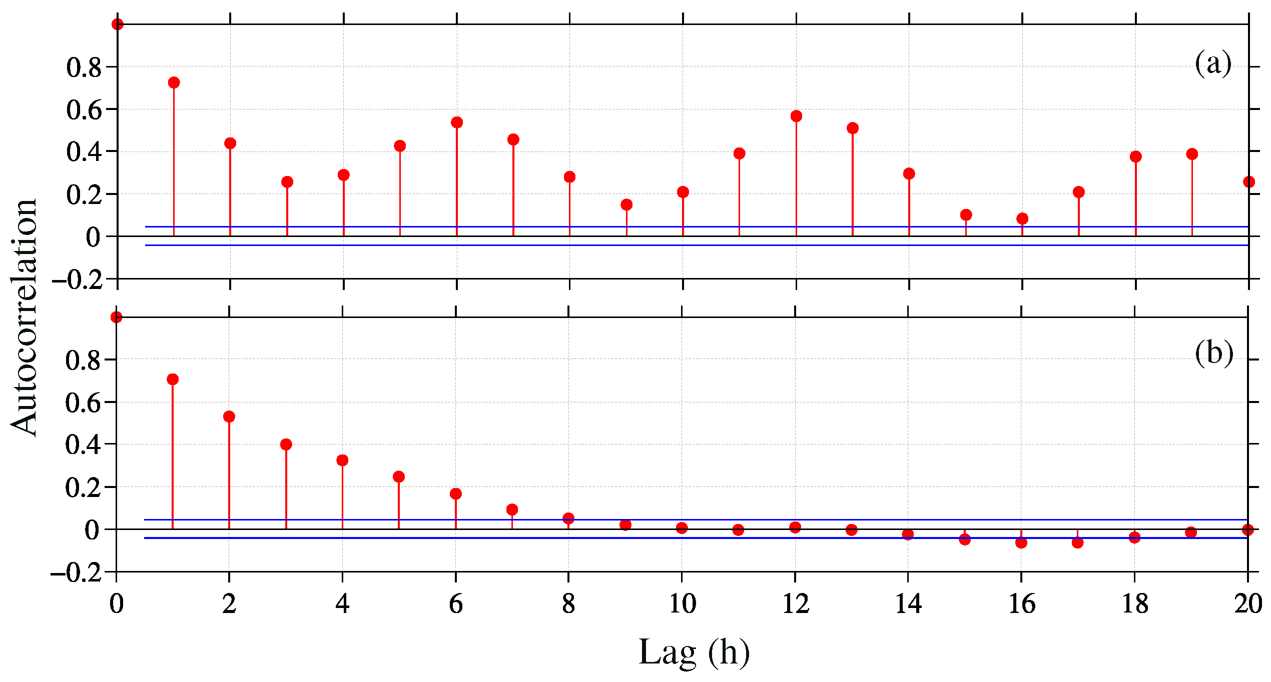
The different results obtained when comparing the radar directional spread to the ADCPs or the wave buoy appear to be related to a stronger tidal modulation on the estimates obtained with the latter instrument, which showed variations of up to 20 in 6-h cycles. Although the wave spread obtained from the radar and the ADCP measurements also showed signs of tidal modulation, the variations were not as significant as in the buoy’s results. This is evidenced by the results of the autocorrelation function of the differences between the wave buoy and the ADCP-E directional spread, plotted in Figure 11a together with the autocorrelation of the differences between the radar spread at equivalent positions (Figure 11b). The residuals obtained from the in situ measurements show a clear tidal signal, with peaks in correlation every 6 h, which is not observed when comparing the radar’s spread measured at the same locations. Using the ADCP-W measurements produced the same outcome (not shown). This suggests that the differences between the wave buoy and the ADCPs are in fact caused by the tidal current.
Six-hour modulation cycles in buoy-measured mean directional spreading were also reported in [47] for the same study area, where they observed a correlation between wave spread and current intensity, characterised by minimum values during slack water, which then increased during the flood and ebb phases of the tide. Both our wave buoy, and the devices used in [47] were deployed in deeper water than our ADCPs, located at sites where the water column was about 20 m shallower than at the buoy’s location. Therefore, the effects of refraction in reducing directional spread might be responsible for the lower values measured by the ADCPs. However, differences in the measuring techniques themselves, as well as in their processing approaches might also be responsible of the differing results. In the presence of background currents, the gain applied to transfer the ADCP subsurface measurements to surface displacement will be overestimated if the value of the current is not taken into account in the calculations. To avoid this issue, the measured velocity data were used in the wave dispersion equation when calculating the ADCP directional spectra. This avoids the energy overestimation, but might also mean the calculated values are not strictly comparable to the buoy’s or the radar’s results.
Finally, irrespective of the parameter studied, the least satisfactory results were generally found when comparing the ADCP-W and radar measurements at that location. This was found to be related to the presence of spurious energy at the low frequencies of the radar spectra. This is due to the modification of the beam pattern as it is steered away from its boresight. Both the width of the main lobe and its sidelobe levels increase, degrading azimuthal resolution and increasing the sensitivity to unwanted signal returns from areas outside the main lobe, respectively. The latter becomes particularly significant when the currents vary across the radar coverage, and can completely hinder wave estimation.
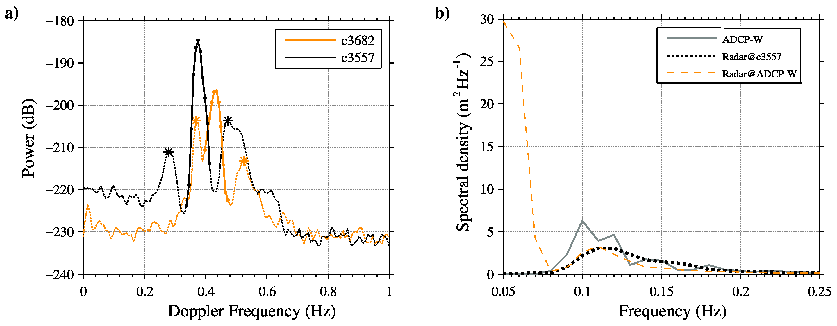
Figure 12 a shows an example of the above. The figure depicts two Doppler spectra measured at 28 km range from Perranporth and different steering angles. In it, it is possible to see how the Bragg peak of the spectrum obtained at 14.6 (cell 3757) from Perranporth’s normal appears as part of the signal obtained at 45 (cell 3682), where the ADCP-W was deployed. As explained in [49], when the differences in first-order Doppler shifts along the same range are large, the Bragg peaks originating from directions other than that of the main lobe can be incorrectly identified as second order structure, and result in artificially large low frequency components in the estimated ocean wave spectrum, as observed in our results, or in [50].
5. Conclusions
HF radars allow measuring the wave directional spectrum from the coast and at relatively high spatial and temporal resolutions. Unlike traditional methods such as wave buoys, they provide a spatial snapshot of the wave field every few minutes, which is very useful in studying the spatiotemporally heterogeneous waters of the coastal seas. Although the most important factor to get good wave estimates from HF radar seems to be the quality of the signal, the algorithm used to convert such signal into ocean wave spectra is also relevant. In this study, we presented an evaluation of the Seaview algorithm [23], which enables the measurement of the wave directional spectrum from HF radar Doppler spectra. The radar results were compared against measurements acquired by three in situ devices deployed at depths that ranged between 33 and 53 m. The qualitative analysis of the directional spectra produced by the inversion algorithm evidenced high concordance between the radar and in situ results for different sea states. Comparisons of radar and in situ-derived wave parameters extracted from the bulk of the spectra resulted in correlations above 0.9 for the significant wave height and energy period, and above 0.79 for the mean direction, at two of the three locations examined. The remaining location, which presented poorer statistics when compared to the in situ measurements, was found to be affected from spurious energy at the low frequencies of the spectra, resulting from contamination of other steering angles. Increased levels of antenna sidelobes at high angles from the radar’s boresight, combined with surface current heterogeneity along a range cell were identified as the source of this problem. A careful analysis of the surface current at the site, along with the examination of antenna patterns are therefore essential to delimit the area where accurate wave results can be expected.
The main drivers of previously reported inaccuracies in the algorithm’s results, usually related to short measuring periods and a limitation of the theory underpinning the inversion in high sea states, have not been found to have a significant effect on the results. This suggests that the integration time used to calculate the radar’s directional spectra, and the chosen transmitting frequency are well suited to measure the wave climate of the area. Nonetheless, adding a higher transmitting frequency would allow measuring low sea states, which with the current configuration resulted in data gaps.
Having established its accuracy, it seems that at present one of the main drawbacks of the method is the data return, which did not exceed 55% over the eight-month period studied here. Together with the above-mentioned possibility of adding a higher transmitting frequency to measure low sea states, improvement of the SNR, noise cancelling techniques, and a dedicated maintenance of the radars are possibly the essential requirements to increase the data return and enable the use of HF radar wave spectra at operational level.
Author Contributions
Conceptualization, G.L. and D.C.C.; Methodology, G.L. and D.C.C.; Writing—Original Draft Preparation, G.L.; and Writing—Review and Editing, D.C.C. and G.L.
Funding
This research was supported by the School of Marine Science and Engineering at Plymouth University, the Natural Environment Research Council (Grant NE/J004219/1) and MARINET, a European Community—Research Infrastructure Action under the FP7 Programme.
Acknowledgments
The authors thank Megan Sheridan, Davide Magagna and Peter Ganderton for their involvement in the deployment of the devices which provided the in situ data used in this work. We are also grateful to all of the Plymouth University Coastal Processes Research Group members, who at some point helped with the maintenance of the radar sites. We also express our gratitude to the anonymous reviewers for their helpful comments and suggestions.
Conflicts of Interest
The authors declare no conflict of interest.
References
- Fujii, S.; Heron, M.L.; Kim, K.; Lai, J.W.; Lee, S.H.; Wu, X.; Wu, X.; Wyatt, L.R.; Yang, W.C. An overview of developments and applications of oceanographic radar networks in Asia and Oceania countries. Ocean Sci. J. 2013, 48, 69–97. [Google Scholar] [CrossRef]
- Roarty, H.; Glenn, S.; Kohut, J.; Gong, D.; Handel, E.; Rivera, E.; Garner, T.; Atkinson, L.; Brown, W.; Jakubiak, C.; et al. Operation and application of a regional high-drequency radar network in the mid-atlantic bight. Marine Technol. Soc. J. 2010, 44, 133–145. [Google Scholar] [CrossRef]
- Rubio, A.; Mader, J.; Corgnati, L.; Mantovani, C.; Griffa, A.; Novellino, A.; Quentin, C.; Wyatt, L.; Schulz-Stellenfleth, J.; Horstmann, J.; et al. HF radar activity in European coastal seas: Next steps toward a pan-European HF radar network. Front. Mar. Sci. 2017, 4, 8. [Google Scholar] [CrossRef]
- Lorente, P.; Sotillo, M.G.; Aouf, L.; Amo-Baladrón, A.; Barrera, E.; Dalphinet, A.; Toledano, C.; Rainaud, R.; De Alfonso, M.; Piedracoba, S.; et al. Extreme Wave Height Events in NW Spain: A Combined Multi-Sensor and Model Approach. Remote Sens. 2018, 10. [Google Scholar] [CrossRef]
- Lorente, P.; Basañez Mercader, A.; Piedracoba, S.; Perez-Muñuzuri, V.; Montero, P.; Alvarez-Fanjul, E. Long-term skill assessment of SeaSonde radar-derived wave parameters in the Galician coast (NW Spain). Int. J. Remote Sens. 2019. [Google Scholar] [CrossRef]
- Saviano, S.; Kalampokis, A.; Zambianchi, E.; Uttieri, M. A year-long assessment of wave measurements retrieved from an HF radar network in the Gulf of Naples (Tyrrhenian Sea, Western Mediterranean Sea). J. Oper. Oceanogr. 2019, 12, 1–15. [Google Scholar] [CrossRef]
- James, C.; Collopy, M.; Wyatt, L.R.; Middleditch, A.; James, C.; Collopy, M.; Wyatt, L.R.; Middleditch, A.; James, C. Suitability of the Southern Australia integrated marine observing system’s ( SA-IMOS ) HF-radar for operational forecasting. J. Oper. Oceanogr. 2019, 12, 1–13. [Google Scholar] [CrossRef]
- Gurgel, K.W.; Essen, H.H.; Kingsley, S.P. High-frequency radars: Physical limitations and recent developments. Coast. Eng. 1999, 37, 201–218. [Google Scholar] [CrossRef]
- Lipa, B. Derivation of directional ocean-wave spectra by integral inversion of second-order radar echoes. Radio Sci. 1977, 12, 425–434. [Google Scholar] [CrossRef]
- Wyatt, L.R. A relaxation method for integral inversion applied to HF radar measurement of the ocean wave directional spectrum. Int. J. Remote Sens. 1990, 11, 1481–1494. [Google Scholar] [CrossRef]
- Howell, R.; Walsh, J. Measurement of ocean wave spectra using narrow-beam HF radar. IEEE J. Ocean. Eng. 1993, 18, 296–305. [Google Scholar] [CrossRef]
- Hisaki, Y. Nonlinear inversion of the integral equation to estimate ocean wave spectra from HF radar. Radio Sci. 1996, 31, 25–39. [Google Scholar] [CrossRef]
- Hashimoto, N.; Tokuda, M. A Bayesian approach for estimation of directional wave spectra with HF radar. Coast. Eng. J. 2003, 41, 137–149. [Google Scholar] [CrossRef]
- Hisaki, Y. Development of HF radar inversion algorithm for spectrum estimation (HIAS). J. Geophys. Res. Oceans 2015, 120, 1725–1740. [Google Scholar] [CrossRef]
- Barrick, D.E. Extraction of wave parameters from measured HF radar sea-echo Doppler spectra. Radio Sci. 1977, 12, 415–424. [Google Scholar] [CrossRef]
- Wyatt, L.R. Significant waveheight measurement with HF radar. Int. J. Remote Sens. 1988, 9, 1087–1095. [Google Scholar] [CrossRef]
- Wyatt, L.R. An evaluation of wave parameters measured using a single HF radar system. Can. J. Remote Sens. 2002, 28, 205–218. [Google Scholar] [CrossRef]
- Maresca, J.W.; Evans, M.W.; Georges, T.M. Measuring rms wave spectra using narrow-beam HF radar. IEEE J. Ocean. Eng. 1980, 18, 295–305. [Google Scholar]
- Heron, S.F.; Heron, M.L. A comparison of algorithms for extracting significant wave height from HF radar ocean backscatter spectra. J. Atmos. Ocean. Technol. 1998, 15, 1157–1163. [Google Scholar] [CrossRef]
- Essen, H.H.; Gurgel, K.W.; Schlick, T. Measurement of ocean wave height and direction by means of HF radar: An empirical approach. Deutsche Hydrographische Zeitschrift 2007, 51, 369–383. [Google Scholar] [CrossRef]
- Gurgel, K.W.; Essen, H.H.; Schlick, T. An empirical method to derive ocean waves from second-order Bragg scattering: Prospects and limitations. IEEE J. Ocean. Eng. 2006, 31, 804–811. [Google Scholar] [CrossRef]
- Alattabi, Z.; Cahl, D.; Voulgaris, G. Swell and wind wave inversion using a single Very High Frequency (VHF) radar. J. Atmos. Ocean Technol. 2019. [Google Scholar] [CrossRef]
- Wyatt, L.R. Limits to the inversion of HF radar backscatter for ocean wave measurement. J. Atmos. Ocean. Technol. 2000, 17, 1651–1665. [Google Scholar] [CrossRef]
- Wyatt, L.R.; Thompson, S.P.; Burton, R.R. Evaluation of high frequency radar wave measurement. Coast. Eng. 1999, 37, 259–282. [Google Scholar] [CrossRef]
- Wyatt, L.R.; Green, J.J.; Gurgel, K.W.; Nieto Borge, J.C.; Reichert, K.; Hessner, K.; Günther, H.; Rosenthal, W.; Saetra, O.; Reistad, M. Validation and intercomparisons of wave measurements and models during the EuroROSE experiments. Coast. Eng. 2003, 48, 1–28. [Google Scholar] [CrossRef] [Green Version]
- Wyatt, L.R.; Green, J.J.; Middleditch, A. Directional spectra comparisons between HF radar and a wave model. In Proceedings of the IEEE Working Conference on Current Measurement Technology, Charleston, SC, USA, 17–19 March 2008; pp. 211–216. [Google Scholar] [CrossRef]
- Wyatt, L.R.; Green, J.J.; Middleditch, A. HF radar data quality requirements for wave measurement. Coast. Eng. 2011, 58, 327–336. [Google Scholar] [CrossRef]
- Wyatt, L.R.; Green, J.J.; Middleditch, A. Signal sampling impacts on HF radar wave measurement. J. Atmos. Ocean. Technol. 2009, 26, 793–805. [Google Scholar] [CrossRef]
- Voulgaris, G.; Haus, B.K.; Work, P.; Shay, L.K.; Seim, H.E.; Weisberg, R.H.; Nelson, J.R. Waves initiative within SEACOOS. Mar. Technol. Soc. J. 2009, 42, 68–80. [Google Scholar] [CrossRef]
- Savidge, D.; Amft, J.; Gargett, A.; Archer, M.; Conley, D.; Voulgaris, G.; Wyatt, L.; Gurgel, K.W. Assessment of WERA long-range HF-radar performance from the user’s perspective. In Proceedings of the 2011 IEEE/OES/CWTM 10th Working Conference on Current, Waves and Turbulence Measurement, CWTM 2011, Monterey, CA, USA, 20–23 March 2011; pp. 31–38. [Google Scholar] [CrossRef]
- Halcrow Group Limited Wave Hub Development Phase Coastal Processes Study Report; Technical Report; South West of England Regional Development Agency: Exeter, UK, 2006.
- Department of Energy & Climate Change. UK Offshore Energy Strategic Environmental Assessment OESEA3 Non-Technical Summary; Technical Report; Department of Energy and Climate Change: London, UK, 2016.
- Gurgel, K.W.; Schlick, T. Compatibility of FMCW modulated HF surface wave radars with radio services. In Proceedings of the International Radar Symposium, IRS 2007, Cologne, Germany, 5–7 September 2007; pp. 255–258. [Google Scholar]
- Weber, B.L.; Barrick, D.E. On the nonlinear theory for gravity waves on the ocean’s surface. part I: Derivations. J. Phys. Oceanogr. 2002, 7, 3–10. [Google Scholar] [CrossRef]
- Middleditch, A.; Cosoli, S. The Australian coastal ocean radar network: Temporal and spatial scales of HF radar wave data. In Proceedings of the IEEE OCEANS 2016, Shanghai, China, 10–13 April 2016; pp. 1–8. [Google Scholar] [CrossRef]
- Kuik, A.J.; van Vledder, G.P.; Holthuijsen, L.H. A Method for the routine analysis of pitch-and-roll buoy wave data. J. Phys. Oceanogr. 2002, 18, 1020–1034. [Google Scholar] [CrossRef]
- Krogstad, H.E. Maximum likelihood estimation of ocean wave spectra from general arrays of wave gauges. Model. Identif. Control 1988, 9, 81–97. [Google Scholar] [CrossRef] [Green Version]
- Teledyne RD Instruments Inc. WAVES PRIMER: Wave Measurements and the RDI ADCP Waves Array Technique; Technical Report; Teledyne RD Instruments Inc.: Poway CA, USA, 2013. [Google Scholar]
- Brodtkorb, P.A.; Johannesson, P.; Lindgren, G.; Rychlik, I.; Ryden, J.; Sjo, E. WAFO—A MATLAB toolbox for random waves and loads. In Proceedings of the Tenth (2000) International Offshore and Polar Engineering Conference, Seattle, WA, USA, 28 May–2 June 2000; Volume 3, pp. 343–350. [Google Scholar]
- Hashimoto, N. Analysis of the Directional Wave Spectrum From Field Data; World Scientific: Singapore, 2010; Volume 3, pp. 103–143. [Google Scholar]
- Lopez, G.; Conley, D.C.; Greaves, D. Calibration, validation, and analysis of an empirical algorithm for the retrieval of wave spectra from HF radar sea echo. J. Atmos. Ocean. Technol. 2016, 33, 245–261. [Google Scholar] [CrossRef]
- Bowers, J.A.; Morton, I.D.; Mould, G.I. Directional statistics of the wind and waves. Appl. Ocean Res. 2000, 22, 13–30. [Google Scholar] [CrossRef]
- Krogstad, H.E.; Wolf, J.; Thompson, S.P.; Wyatt, L.R. Methods for intercomparison of wave measurements. Coast. Eng. 1999, 37, 235–257. [Google Scholar] [CrossRef]
- Strong, B.; Brumley, B.; Terray, E.; Stone, G. The performance of ADCP-derived directional wave spectra and comparison with other independent measurements. In Proceedings of the OCEANS 2000 MTS/IEEE, Providence, RI, USA, 11–14 September 2002; Volume 2, pp. 1195–1203. [Google Scholar] [CrossRef]
- Green, J.J.; Wyatt, L.R. Row-action inversion of the Barrick-Weber equations. J. Atmos. Ocean. Technol. 2006, 23, 501–510. [Google Scholar] [CrossRef]
- Wyatt, L.R. Measuring the ocean wave directional spectrum ‘First Five’ with HF radar. Ocean Dyn. 2019, 69, 123–144. [Google Scholar] [CrossRef]
- Saulnier, J.B.; Maisondieu, C.; Ashton, I.; Smith, G.H. Refined sea state analysis from an array of four identical directional buoys deployed off the Northern Cornish coast (UK). Appl. Ocean Res. 2012, 37, 1–21. [Google Scholar] [CrossRef] [Green Version]
- Work, P.A. Nearshore directional wave measurements by surface-following buoy and acoustic Doppler current profiler. Ocean Eng. 2008, 35, 727–737. [Google Scholar] [CrossRef]
- Wyatt, L.R.; Liakhovetski, G.; Graber, H.C.; Haus, B.K. Factors affecting the accuracy of SHOWEX HF radar wave measurements. J. Atmos. Ocean. Technol. 2005, 22, 847–859. [Google Scholar] [CrossRef]
- Middleditch, A. Spectral Analysis in High Frequency Radar Oceanography. PhD Thesis, University of Sheffield, Sheffield, UK, 2006. [Google Scholar]
Figure 1.
Study area: (right) the red rectangle demarcates the area shown in left figure, (left) radar stations (black circles), their coverage (50 km radius fans) and measuring grid. Depth contours are also shown and expressed in meters. The temporal data coverage of each radar cell is shown as a percentage of the time each cell had inverted wave data. The in situ mooring devices are also depicted: wave buoy (star), ADCP-W (inverted triangle) and ADCP-E (triangle). The grey rectangle delimits the Wave Hub test site for marine renewable energy devices.

Figure 2.
Radar wave parameters co-located with the wave buoy (red star), the ADCP-W (dark blue dots) and ADCP-E (light blue crosses) from April to November 2012 (a) significant wave height and wind speed (grey line); (b) energy period; (c) wave direction (direction of approach) and wind direction (grey line); and (d) mean directional spreading.

Figure 3.
Same as previous figure, but showing the in situ-measured wave parameters.

Figure 4.
Correlation coefficient and RMSE obtained from the comparison between radar- and in situ-measured wave parameters. The three in situ devices are represented by a different color: buoy (blue), ADCP-E (grey) and ADCP-W (orange). The symbols denote the different wave parameters evaluated: energy period (T; star), mean period (T; square), peak period (T; diamond), significant wave height (H; triangle), mean wave direction (circle), and directional wave spread (spr; inverted triangle). The units of the RMSE values are meters, seconds, and radians for the wave height, period, and direction and wave spreading, respectively. Results are shown for three frequency bands and the full range of available frequencies: (a) 0.05–0.1 Hz; (b) 0.1–0.15 Hz; (c) 0.15–0.25; and (d) 0.05–0.25 Hz.

Figure 5.
Radar and in situ estimates of wave directional spectra on 21 October 2012 at 1000 UTC. The upper panels show the results obtained from the in situ measurements, and the bottom panels show the radar estimates: ADCP-E spectra (a,d); and ADCP-W (b,e). Wave buoy (c,f). The colorbar represents the directional energy density (m/Hz/deg).

Figure 6.
Radar and in situ estimates of one-dimensional spectra, mean direction and directional spreading as a function of frequency on 21 October 2012 at 1000 UTC: (a) ADCP-E (dashed black line and *) and radar (grey line and +); (b) ADCP-W (dashed black line and *) and radar (grey line and +); and (c) buoy (dashed black line and *) and radar (grey line and +).

Figure 7.
As in Figure 5, but for 24 September 2012 at 1100 UTC.
Figure 7.
As in Figure 5, but for 24 September 2012 at 1100 UTC.

Figure 8.
As in Figure 6, but for 24 September 2012 at 1100 UTC.
Figure 8.
As in Figure 6, but for 24 September 2012 at 1100 UTC.

Figure 9.
As in Figure 5, but for 26 October 2012 at 0100 UTC.
Figure 9.
As in Figure 5, but for 26 October 2012 at 0100 UTC.

Figure 10.
As in Figure 6, on 26 October 2012 at 0100 UTC.
Figure 10.
As in Figure 6, on 26 October 2012 at 0100 UTC.

Figure 11.
Autocorrelation function of the time series of the differences between directional spread measured at two locations: (a) autocorrelation of differences between the wave buoy and the ADCP-E directional spread; and (b) autocorrelation of the differences between the radar directional spread estimates obtained at the buoy and ADCP-E sites. The confidence bounds are shown in blue.

Figure 12.
Radar measurement affected by antenna sidelobes: (a) The Doppler spectra measured at 14 (black line) and 45 (orange line) from Perranporth’s normal. The first-order region of each spectrum is emphasized with a full line. The stars indicate the identified second order peaks. (b) The frequency spectra obtained at the same two cells, and measured by the ADCP-W, located at cell 3682.


Table 1.
Summary statistics of the radar and in situ H, T, D and directional spread comparisons calculated over the full range of frequencies (0.05–0.25 Hz), as shown in Figure 4d. The third and fourth columns are the in situ- and radar-measured mean values, respectively. The fifth column is the radar standard deviation normalized by the in situ value, the sixth is the RMSE (meters, seconds and degrees for H, T, D, and spr, respectively), the seventh is the correlation coefficient, and the last column is the number of records.
| Device | Parameter | std | RMSE | R | N | ||
|---|---|---|---|---|---|---|---|
| H | 2.18 | 2.20 | 0.91 | 0.30 | 0.94 | ||
| T | 7.94 | 7.95 | 1.27 | 0.56 | 0.91 | ||
| Buoy | T | 8.92 | 8.81 | 0.99 | 1.72 | 0.73 | 2617 |
| D | 276 | 265 | 1.06 | 22.3 | 0.79 | ||
| spr | 40.4 | 42.75 | 0.76 | 9.22 | 0.25 | ||
| H | 1.91 | 2.04 | 1.16 | 0.37 | 0.92 | ||
| T | 8.07 | 7.77 | 0.83 | 0.59 | 0.93 | ||
| ADCP-E | T | 9.25 | 8.54 | 0.80 | 1.78 | 0.76 | 2366 |
| D | 290 | 276 | 1.14 | 21.2 | 0.87 | ||
| spr | 29.4 | 40.9 | 1.11 | 7.93 | 0.32 | ||
| H | 2.11 | 2.19 | 1.04 | 0.45 | 0.87 | ||
| T | 8.48 | 8.51 | 1.02 | 1.38 | 0.66 | ||
| ADCP-W | T | 9.78 | 9.99 | 1.25 | 3.20 | 0.49 | 2320 |
| D | 284 | 265 | 1.21 | 28.5 | 0.80 | ||
| spr | 26.9 | 43.3 | 1.29 | 7.22 | 0.28 |
© 2019 by the authors. Licensee MDPI, Basel, Switzerland. This article is an open access article distributed under the terms and conditions of the Creative Commons Attribution (CC BY) license (http://creativecommons.org/licenses/by/4.0/).
Share and Cite
MDPI and ACS Style
Lopez, G.; Conley, D.C. Comparison of HF Radar Fields of Directional Wave Spectra Against In Situ Measurements at Multiple Locations. J. Mar. Sci. Eng. 2019, 7, 271. https://doi.org/10.3390/jmse7080271
AMA Style
Lopez G, Conley DC. Comparison of HF Radar Fields of Directional Wave Spectra Against In Situ Measurements at Multiple Locations. Journal of Marine Science and Engineering. 2019; 7(8):271. https://doi.org/10.3390/jmse7080271
Chicago/Turabian StyleLopez, Guiomar, and Daniel C. Conley. 2019. "Comparison of HF Radar Fields of Directional Wave Spectra Against In Situ Measurements at Multiple Locations" Journal of Marine Science and Engineering 7, no. 8: 271. https://doi.org/10.3390/jmse7080271
Note that from the first issue of 2016, this journal uses article numbers instead of page numbers. See further details here.