Model Development and Hindcast Simulations of NOAA’s Integrated Northern Gulf of Mexico Operational Forecast System

Abstract
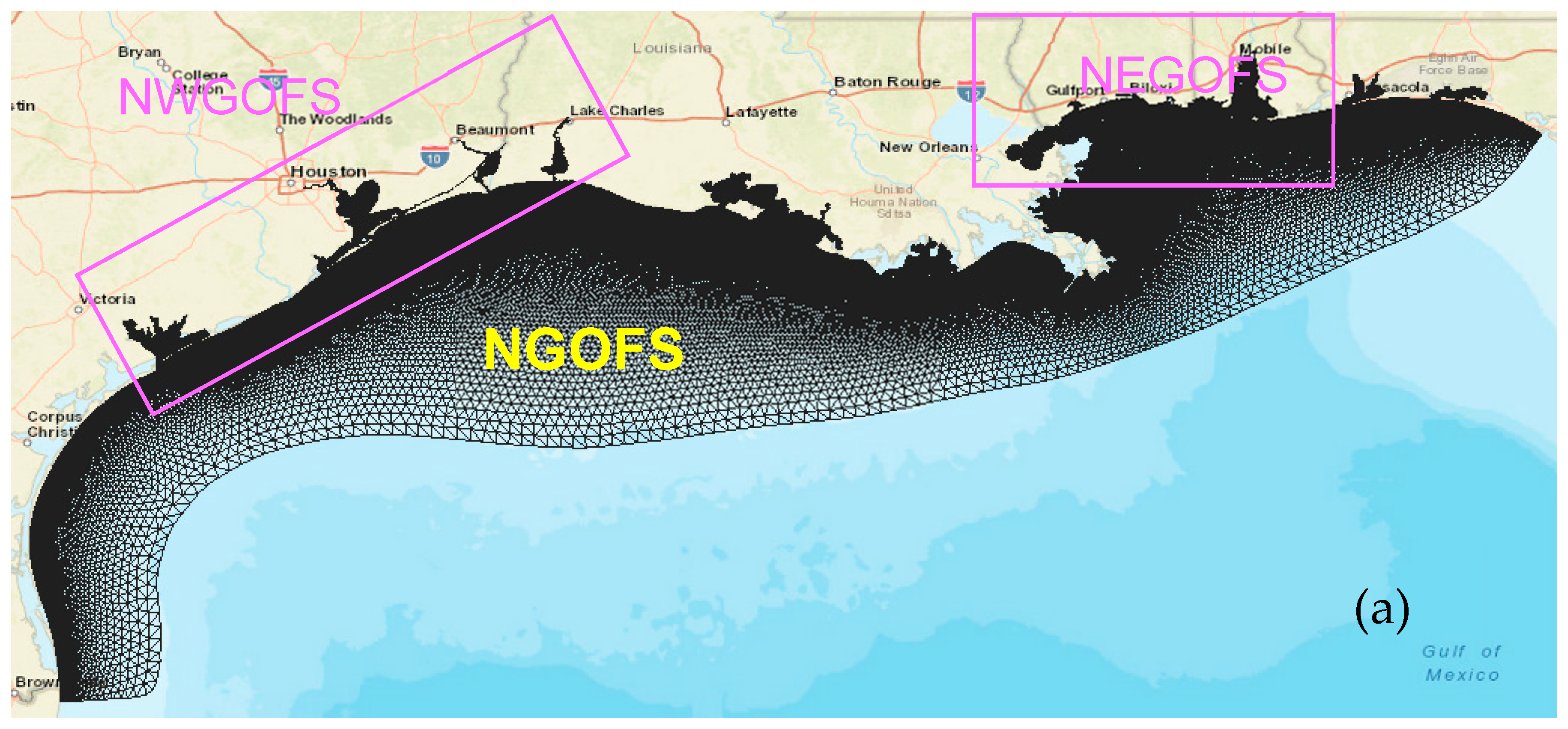
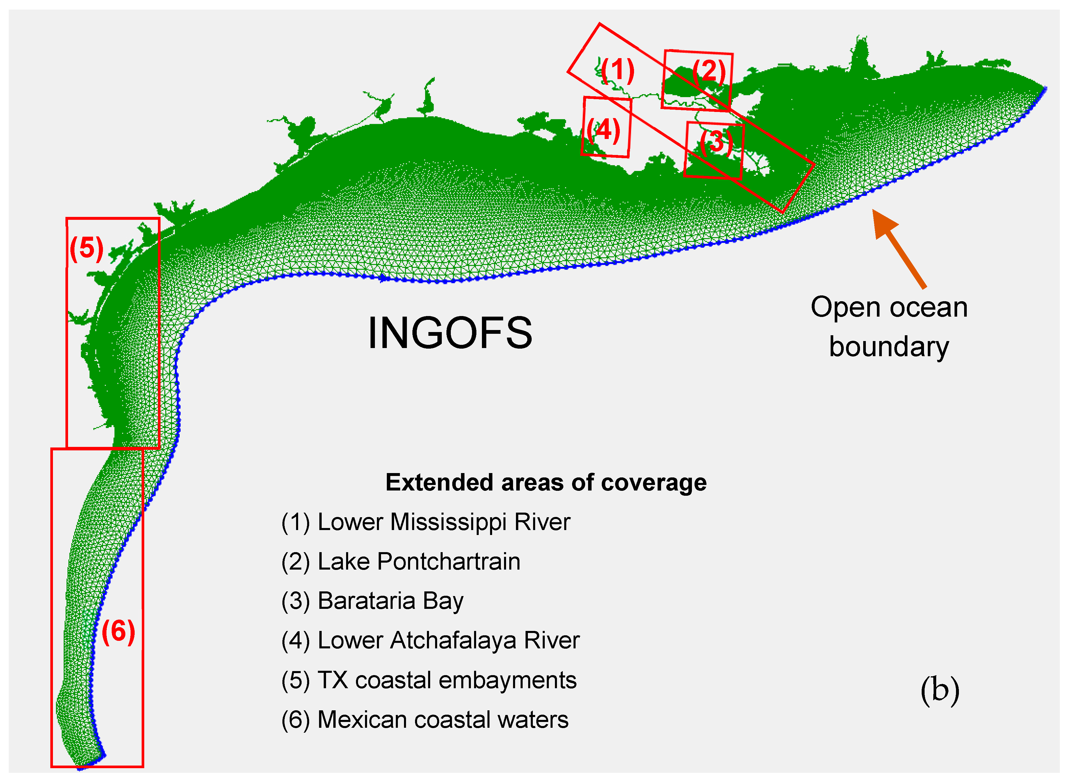
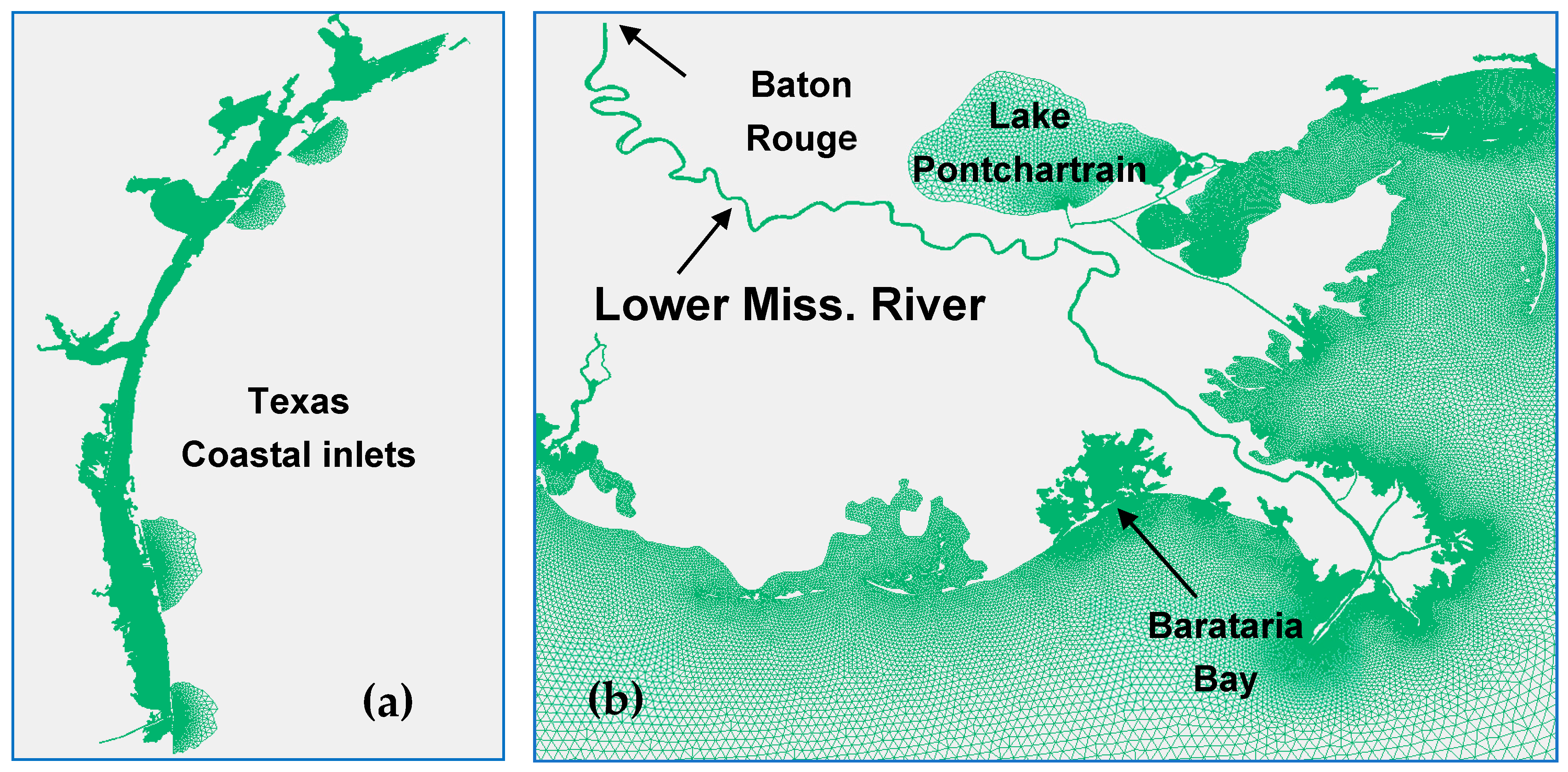
:1. Introduction
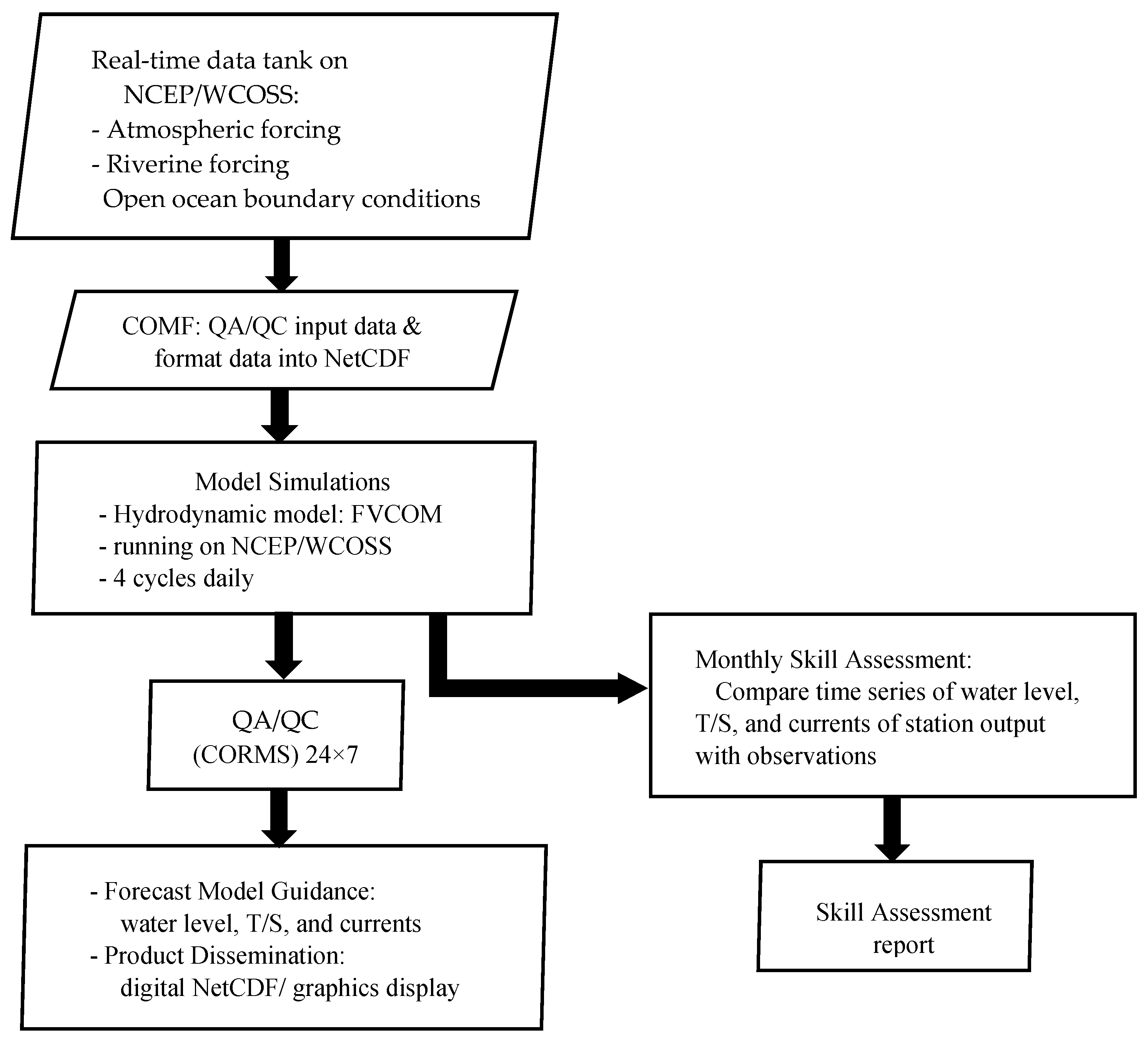
2. Methods
3. Observational Data
4. Results of Hindcast Simulations
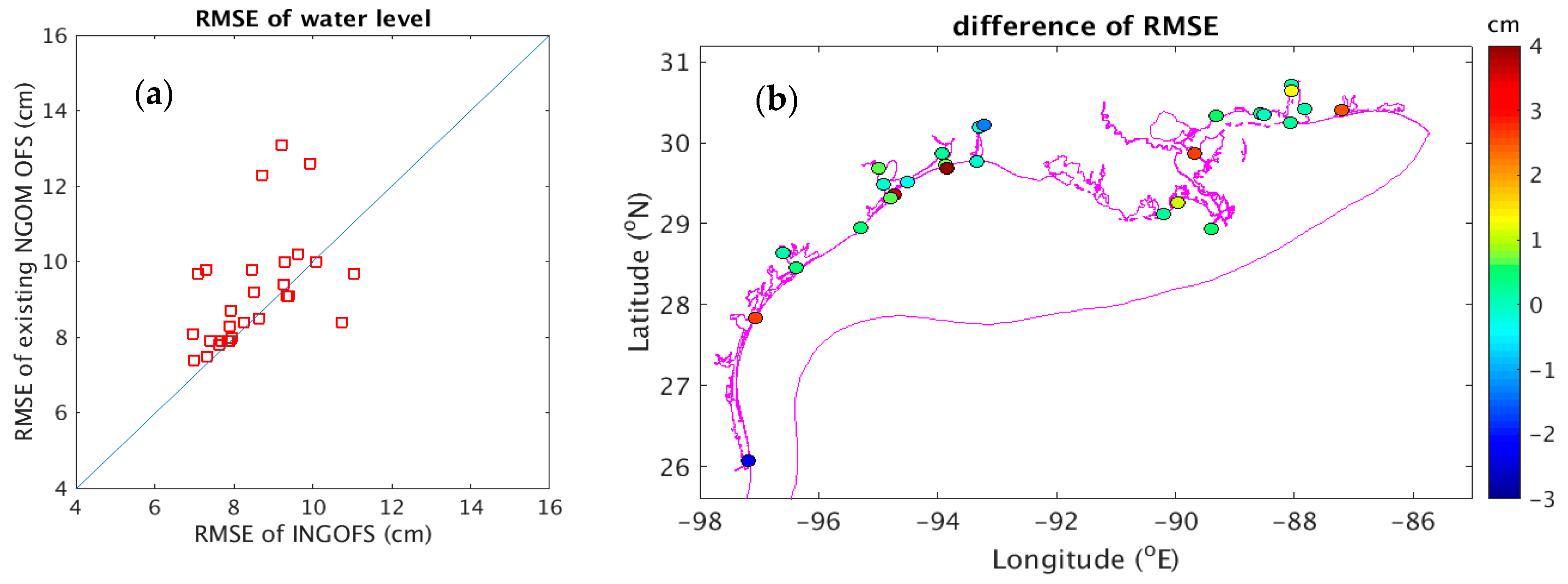
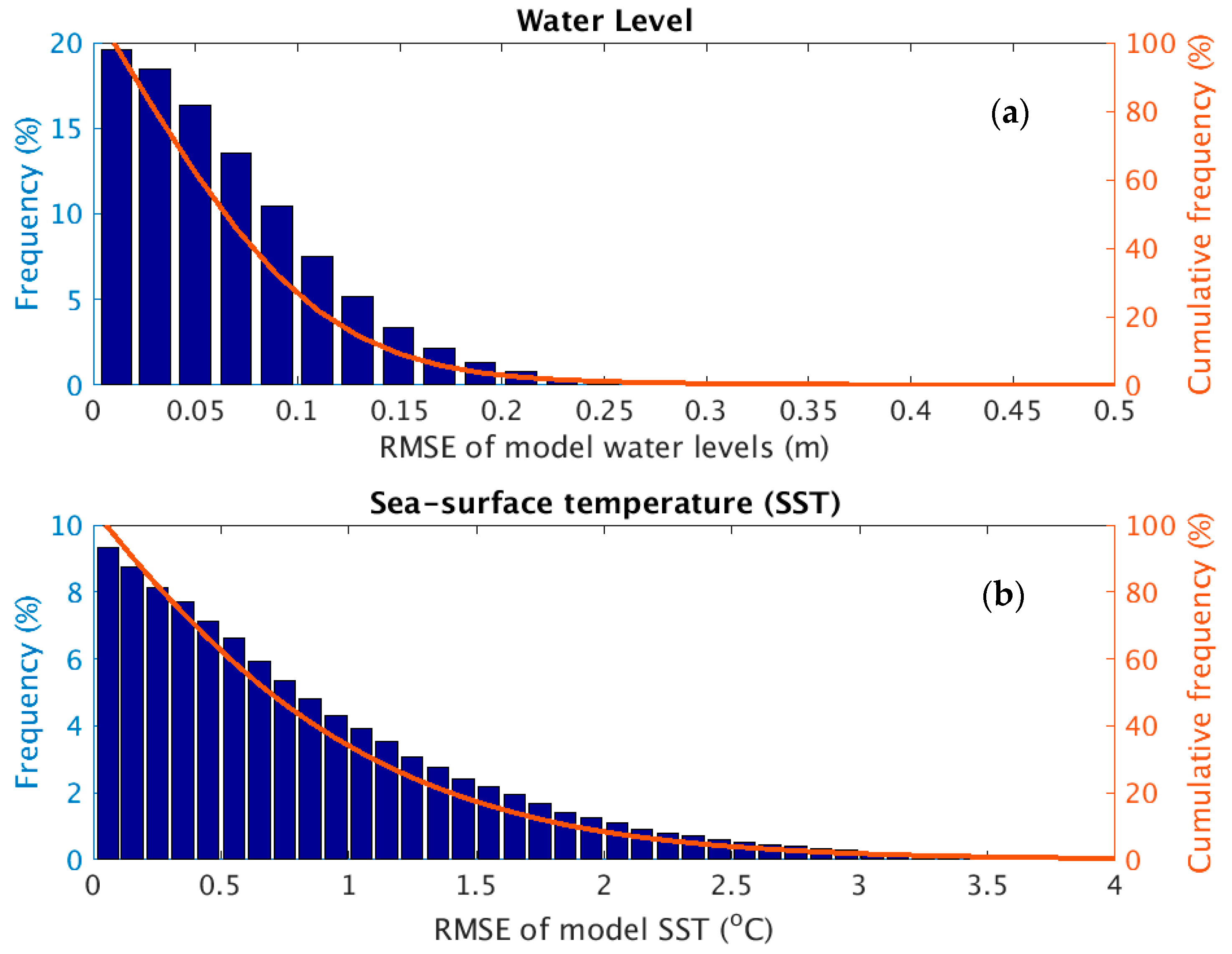
4.1. Water Level
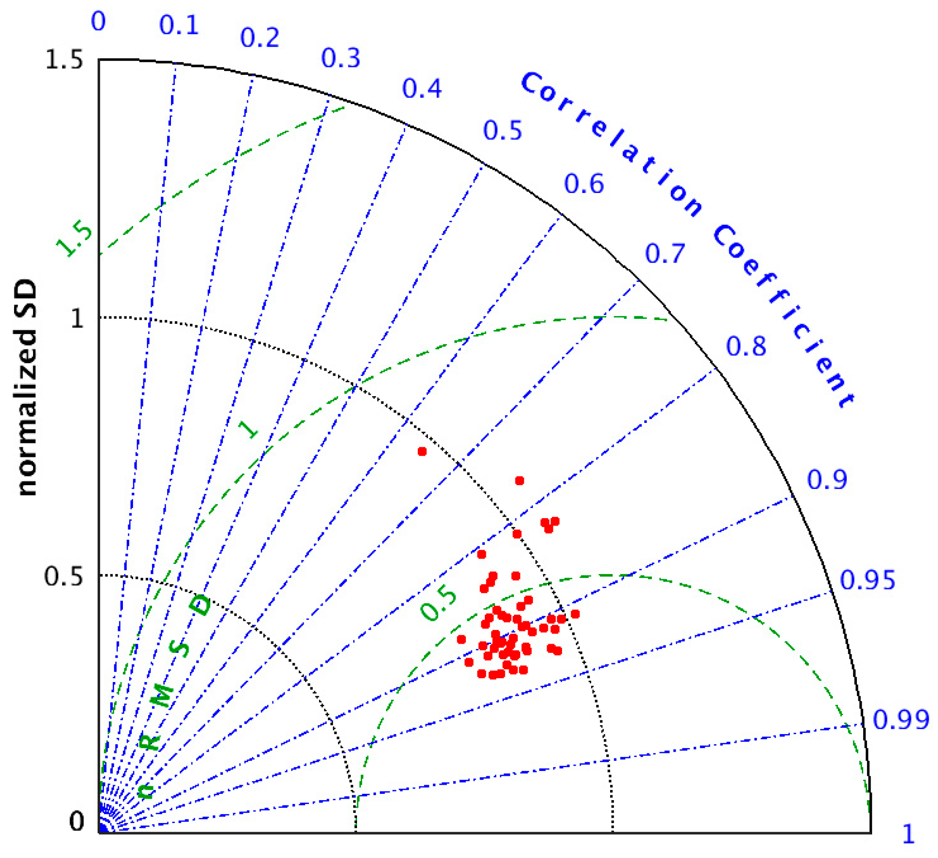
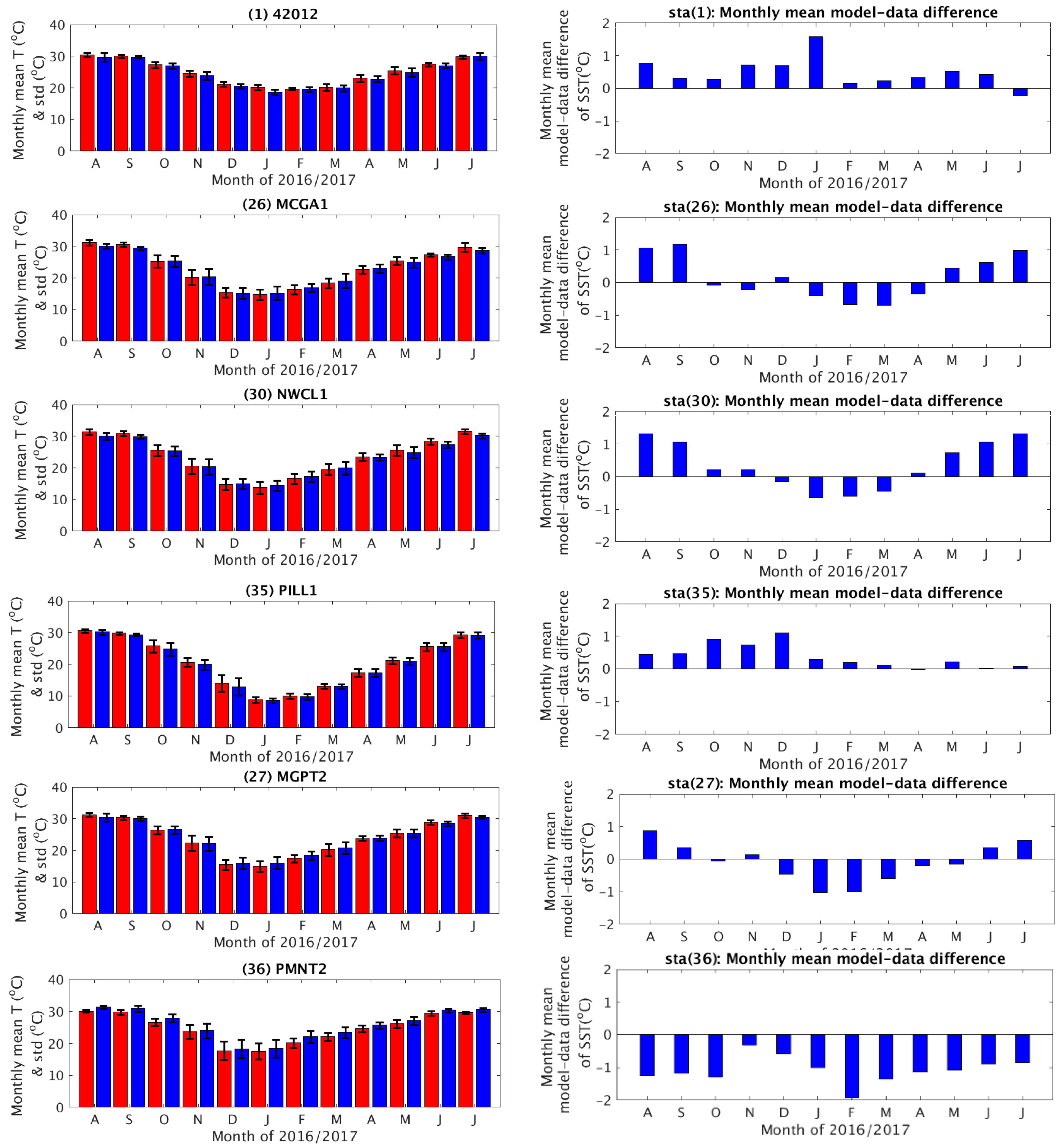
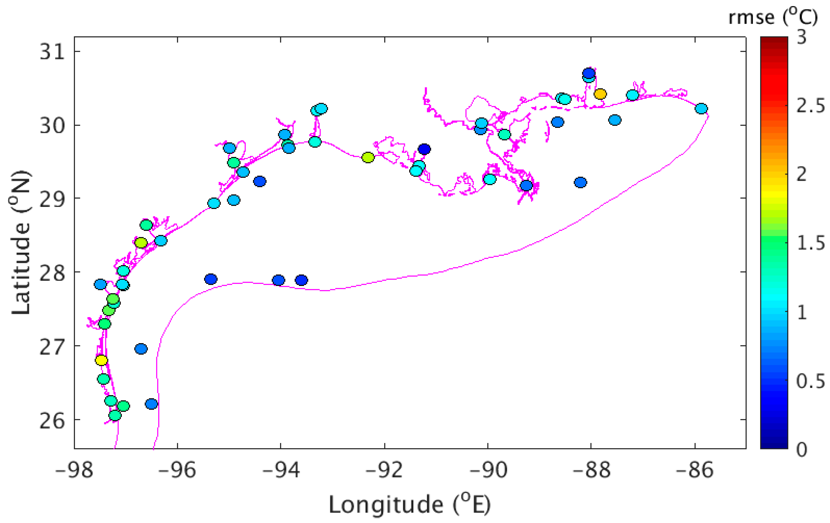
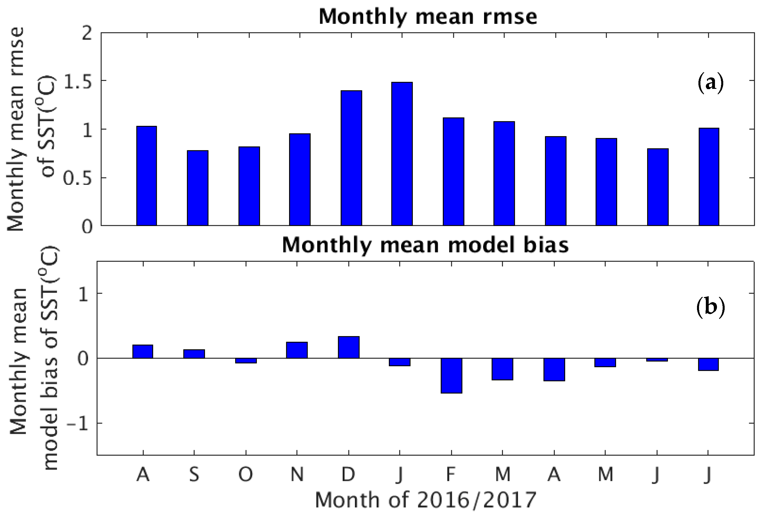
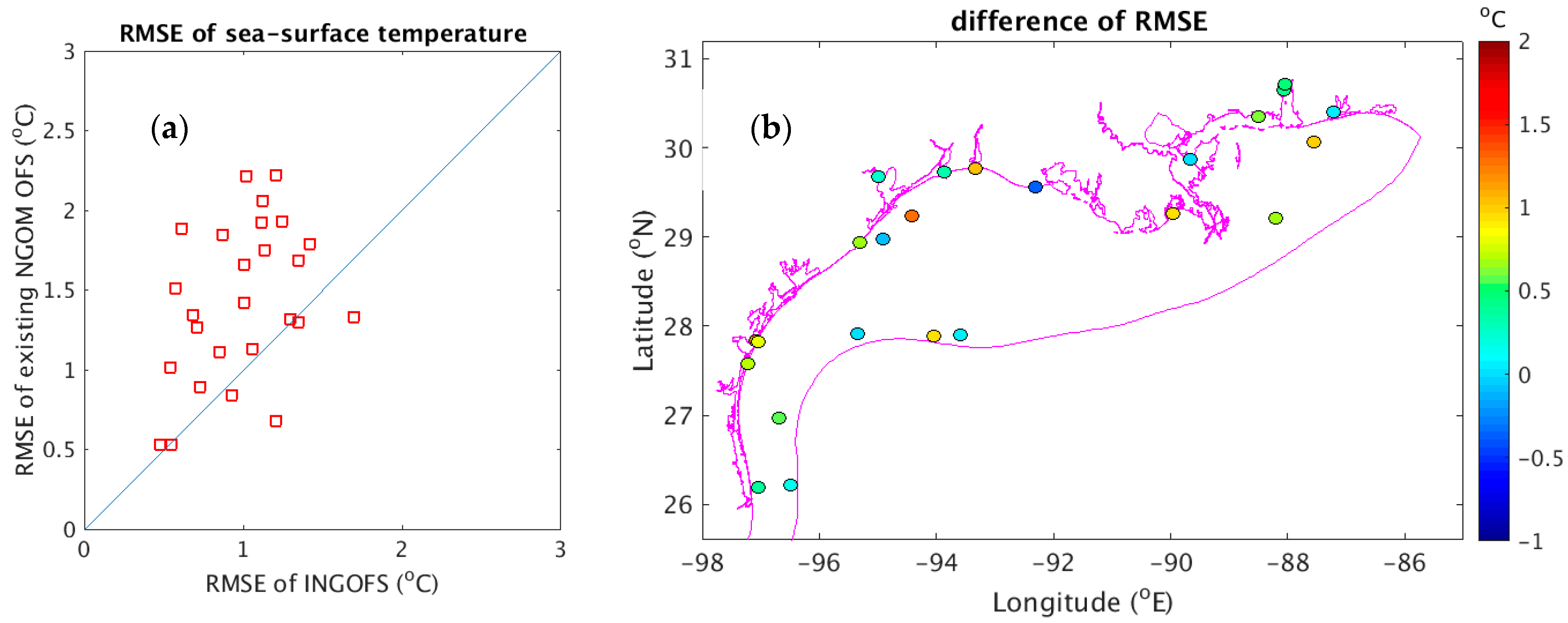
4.2. Sea-Surface Temperature (SST)
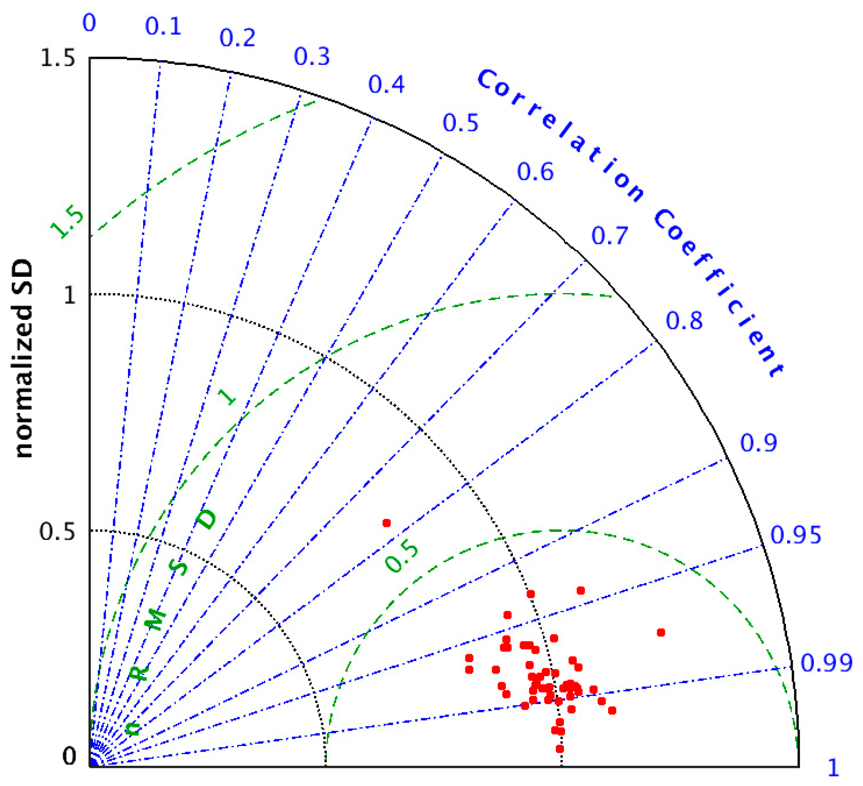
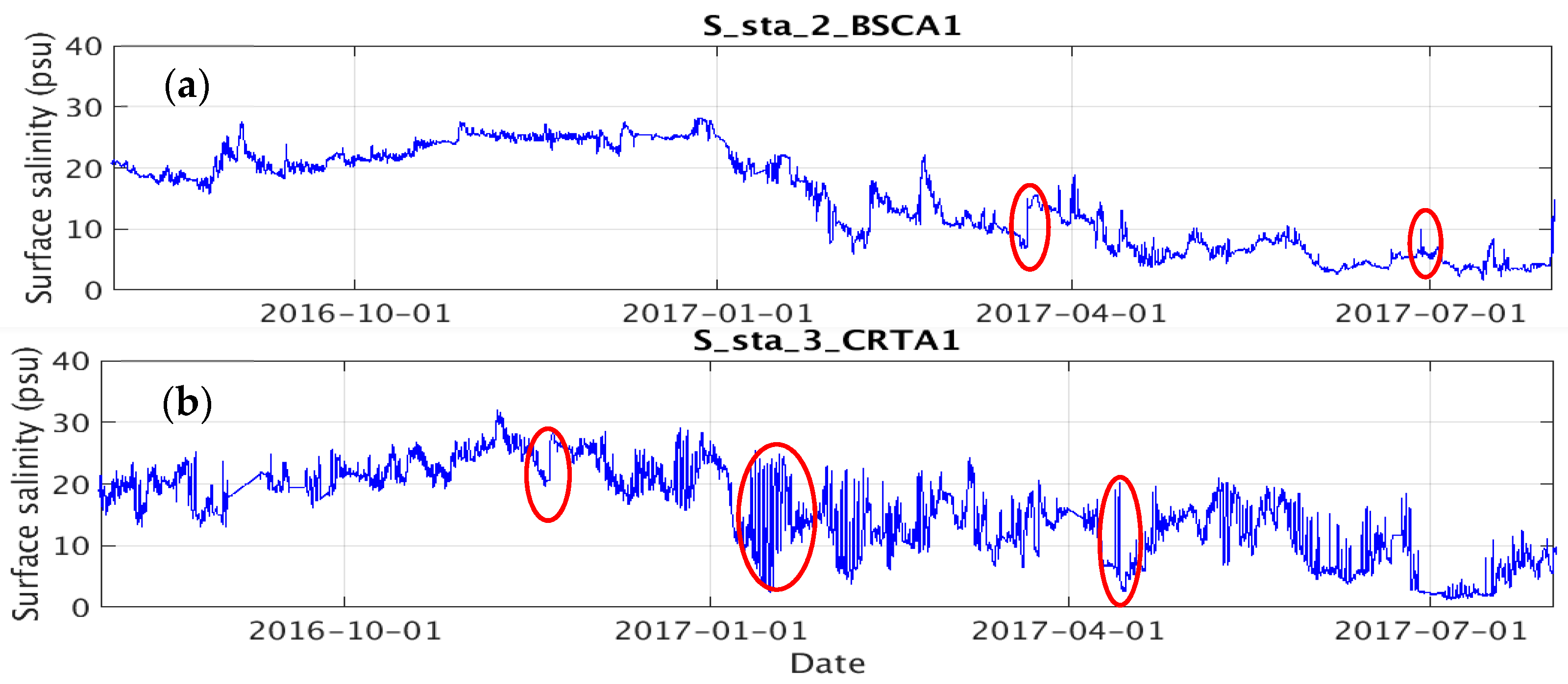
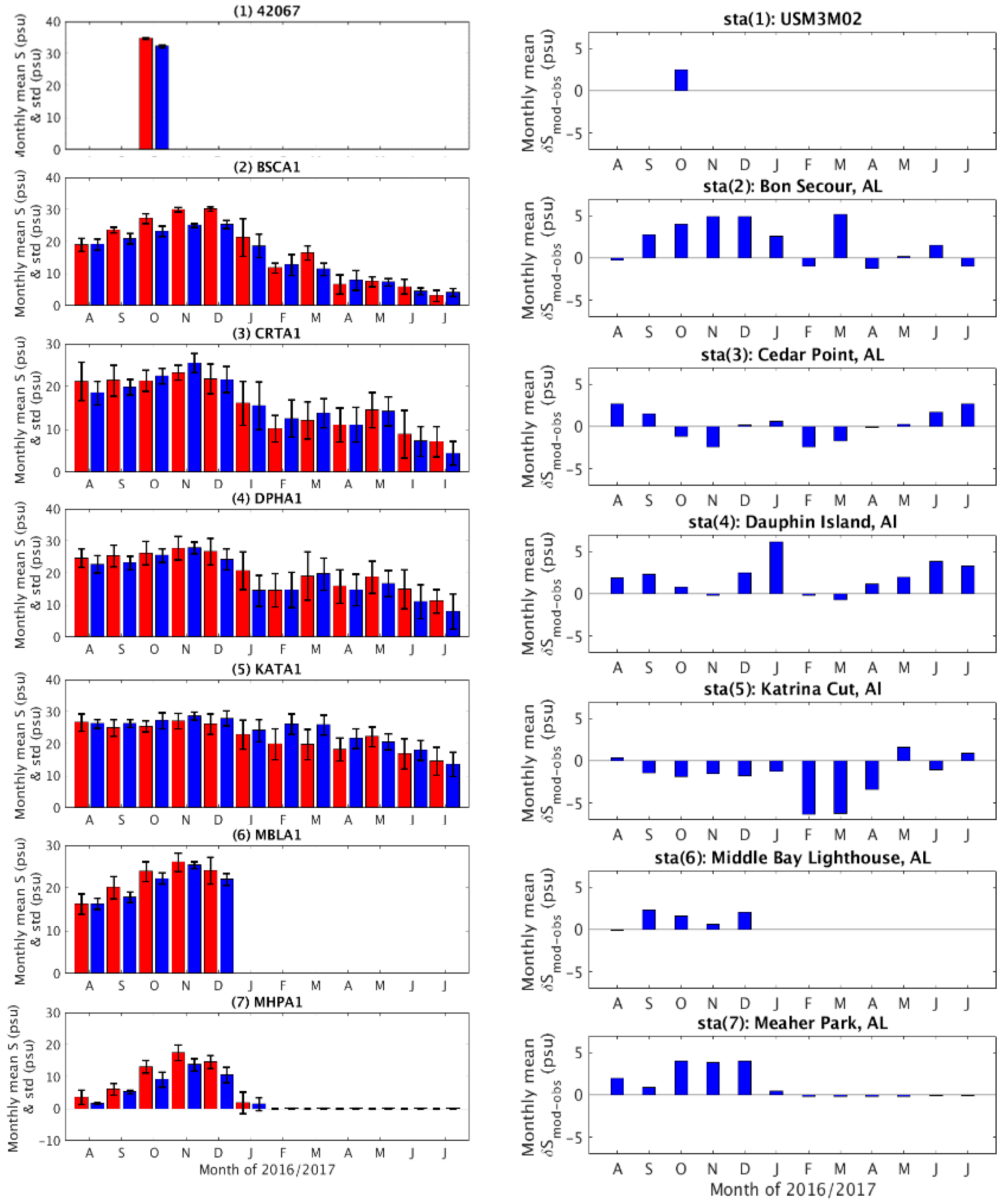
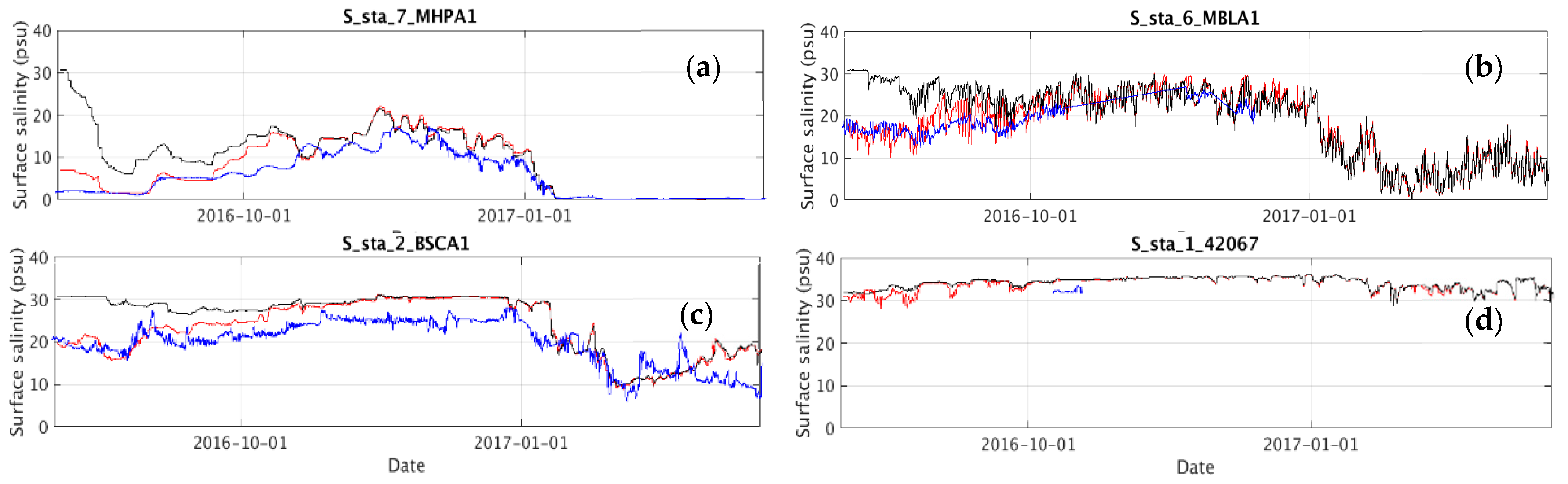
4.3. Sea-Surface Salinity (SSS)
5. Discussion
5.1. Comparison of Model Skills with Other OFS
5.2. Limitation of the RMSE Analysis
6. Summary and Conclusions
Author Contributions
Acknowledgments
Conflicts of Interest
Appendix A

| No. | IDs | Station Names | Longitude (°E) | Latitude (°N) |
|---|---|---|---|---|
| 1 | 8735180 | Dauphin Island | −88.075 | 30.25 |
| 2 | 8735391 | Dog River Bridge | −88.088 | 30.5652 |
| 3 | 8735523 | East Fowl River, Hwy 193 Bridge | −88.1139 | 30.4437 |
| 4 | 8741533 | Pascagoula NOAA Lab, MS | −88.5667 | 30.3583 |
| 5 | 8747437 | St. Louis Bayentrance | −89.3258 | 30.3264 |
| 6 | 8760721 | Pilot Town | −89.2583 | 29.1783 |
| 7 | 8760922 | Pilots Station E, SW Pass, LA | −89.4067 | 28.9317 |
| 8 | 8761305 | Shell Beach, Lake Borgne | −89.6732 | 29.8681 |
| 9 | 8761724 | East Point, Grand Isle | −89.9567 | 29.2633 |
| 10 | 8761927 | New Canal USCG station, Lake Pontchartrain | −90.1134 | 30.0272 |
| 11 | 8762483 | I-10 Bonnet Carre Floodway, TX | −90.39 | 30.0683 |
| 12 | 8764314 | Eugene Island, North of Atchafalaya Bay | −91.3839 | 29.3675 |
| 13 | 8767961 | Bulk Terminal | −93.3007 | 30.1903 |
| 14 | 8768094 | Calcasieu Pass | −93.3429 | 29.7682 |
| 15 | 8770475 | Port Arthur | −93.93 | 29.8667 |
| 16 | 8770570 | Sabine Pass | −93.8701 | 29.7284 |
| 17 | 8770613 | Morgans Point, Barbours Cut | −94.985 | 29.6817 |
| 18 | 8770808 | High Island, ICWW | −94.3903 | 29.5947 |
| 19 | 8770822 | Texas Point, Sabine Pass | −93.8418 | 29.6893 |
| 20 | 8770971 | Rollover Pass | −94.5133 | 29.515 |
| 21 | 8771013 | Eagle Point | −94.9183 | 29.48 |
| 22 | 8771341 | Galveston Bay Entrance, TX | −94.7248 | 29.3573 |
| 23 | 8771450 | GALVESTON, Galveston Channel | −94.7933 | 29.31 |
| 24 | 8771486 | Galveston Railroad Bridge, TX | −94.8967 | 29.3017 |
| 25 | 8771972 | San Luis Pass | −95.1133 | 29.095 |
| 26 | 8773259 | Port Lavaca, TX | −96.6094 | 28.6403 |
| 27 | 8773701 | Port O’Connor, Matagorda Bay | −96.3883 | 28.4517 |
| 28 | 8773767 | Maragorda Bay Entrance Channel, TX | −96.3283 | 28.4267 |
| 29 | 8774513 | Copano Bay, TX, TCOON | −97.0217 | 28.1183 |
| 30 | 8774770 | Rockport, TX | −97.0467 | 28.0217 |
| 31 | 8775237 | Port Aransas, TX | −97.0733 | 27.8383 |
| 32 | 8775296 | USS Lexington, TX | −97.39 | 27.8117 |
| 33 | 8775792 | Packery Channel | −97.2367 | 27.6333 |
| 34 | 8775870 | Corpus Christi | −97.2167 | 27.58 |
| 35 | 8776139 | S. BirdIsland, TX | −97.3217 | 27.48 |
| 36 | 8776604 | Baffin Bay, TX | −97.405 | 27.295 |
| 37 | 8777812 | Rincon Del San Jose, TX | −97.4917 | 26.825 |
| 38 | 8779748 | South Padre Island, TX | −97.1767 | 26.0767 |
| 39 | 8779770 | Port Isabel | −97.215 | 26.06 |
| 40 | 8778490 | Port Mans Field, TX | −97.4217 | 26.555 |
| 41 | 8774230 | Aransas Wildlife Refuge | −96.795 | 28.2283 |
| 42 | 8773037 | Seadrift TCOON, TX | −96.7117 | 28.4083 |
| 43 | 8772447 | USCG Freeport, TX | −95.3017 | 28.9433 |
| 44 | 8770777 | Manchester, Houston Ship Channel | −95.2658 | 29.7263 |
| 45 | 8770733 | Lynchburg Landing, San Jacinto River | −95.0783 | 29.765 |
| 46 | 8770520 | Rainbow Bridge | −93.8817 | 29.98 |
| 47 | 8767816 | Lake Charles | −93.2217 | 30.2236 |
| 48 | 8762075 | Port Fourchon | −90.1993 | 29.1142 |
| 49 | 8741041 | Dock E, Port of Pascagoula | −88.5054 | 30.3477 |
| 50 | 8739803 | Bayou LaBatre Bridge | −88.2477 | 30.4057 |
| 51 | 8738043 | West Fowl River, Hwy 188 bridge | −88.1586 | 30.3766 |
| 52 | 8737048 | MOBILE, Mobile River, State Dock | −88.0433 | 30.7083 |
| 53 | 8736897 | Coast Guard Sector Mobile | −88.0583 | 30.6483 |
| 54 | 8732828 | Weeks Bay, AL | −87.825 | 30.4167 |
| 55 | 8729840 | Pensacola | −87.2111 | 30.4044 |
| No. | IDs | Station Names | Longitude (°E) | Latitude (°N) | Model-Data Difference (°C) |
|---|---|---|---|---|---|
| 1 | 42012 | 44 NM SE of Mobile, Al | −87.555 | 30.065 | 0.48 |
| 2 | 42019 | 60 nm South of Freeport, TX | −95.353 | 27.913 | −0.23 |
| 3 | 42020 | 60 nm SSE of Corpus Christi, TX | −96.694 | 26.968 | −0.01 |
| 4 | 42035 | 22 nm East of Galveston, TX | −94.413 | 29.232 | 0.17 |
| 5 | 42040 | 64 NM South of Dauphin Island, Al | −88.207 | 29.212 | −0.21 |
| 6 | 42043 | GA-252 TABS B | −94.919 | 28.982 | 0.51 |
| 7 | 42044 | PS-1126 TABS J | −97.051 | 26.191 | 0.77 |
| 8 | 42045 | PI-745 TABS K | −96.5 | 26.217 | −0.08 |
| 9 | 42046 | HI-A595 TABS N | −94.037 | 27.89 | −0.27 |
| 10 | 42047 | HI-A389 TABS V | −93.597 | 27.897 | −0.04 |
| 11 | 42067 | USM3M02 | −88.649 | 30.043 | 0.62 |
| 12 | AMRL1 | LAWMA, Amerada Pass, LA | −91.338 | 29.45 | 0.08 |
| 13 | BABT2 | Baffin Bay, TX | −97.405 | 27.297 | −0.57 |
| 14 | BKTL1 | Lake Charles Bulk Terminal, LA | −93.296 | 30.194 | 0.07 |
| 15 | CAPL1 | Calcasieu, La | −93.343 | 29.768 | 0.52 |
| 16 | CARL1 | Carrollton, LA | −90.135 | 29.933 | 0.52 |
| 17 | EINL1 | North of Eugene Island, LA | −91.384 | 29.373 | 0.12 |
| 18 | EPTT2 | Eagle Point, TX | −94.917 | 29.481 | −0.77 |
| 19 | FCGT2 | USCG Freeport, TX | −95.303 | 28.943 | −0.04 |
| 20 | FRWL1 | Fresh Water Canal Locks, La | −92.305 | 29.555 | −0.11 |
| 21 | GISL1 | Grand Isle, LA | −89.958 | 29.265 | −0.42 |
| 22 | GNJT2 | Galveston Bay Entrance (North Jetty), TX | −94.725 | 29.357 | 0.22 |
| 23 | IRDT2 | South Bird Island, TX | −97.322 | 27.48 | −0.58 |
| 24 | LCLL1 | Lake Charles, La | −93.222 | 30.223 | 0.41 |
| 25 | MBET2 | Matagorda Bay Entrance Channel, TX | −96.327 | 28.422 | 0.39 |
| 26 | MCGA1 | Coast Guard Sector Mobile, AL | −88.058 | 30.649 | 0.17 |
| 27 | MGPT2 | Morgans Point, TX | −94.985 | 29.682 | −0.09 |
| 28 | MQTT2 | Bob Hall Pier, Corpus Christi, Tx | −97.217 | 27.58 | −0.08 |
| 29 | NUET2 | Nueces Bay, TX | −97.486 | 27.832 | −0.37 |
| 30 | NWCL1 | New Canal Station, LA | −90.113 | 30.027 | 0.34 |
| 31 | OBLA1 | Mobile State Docks, AL | −88.04 | 30.705 | 0.11 |
| 32 | PACT2 | Packery Channel, TX | −97.237 | 27.634 | −0.34 |
| 33 | PCBF1 | Panama City Beach, FL | −85.88 | 30.213 | 0.36 |
| 34 | PCLF1 | Pensacola, FL | −87.212 | 30.403 | 0.38 |
| 35 | PILL1 | Pilottown, LA | −89.259 | 29.179 | 0.38 |
| 36 | PMNT2 | Port Mansfield, TX | −97.424 | 26.559 | −1.06 |
| 37 | PNLM6 | Pascagoula NOAA Lab, MS | −88.567 | 30.358 | 0.53 |
| 38 | PORT2 | Port Arthur, TX | −93.93 | 29.867 | 0.48 |
| 39 | PTAT2 | Port Aransas, TX | −97.05 | 27.828 | −0.23 |
| 40 | PTIT2 | Port Isabelle, TX | −97.215 | 26.06 | −0.01 |
| 41 | RCPT2 | Rockport, TX | −97.048 | 28.024 | 0.17 |
| 42 | RLIT2 | Realitos Peninsula, TX | −97.285 | 26.262 | −0.21 |
| 43 | RSJT2 | Rincon del San Jose, TX | −97.471 | 26.801 | 0.51 |
| 44 | RTAT2 | Port Aransas, TX | −97.073 | 27.84 | 0.77 |
| 45 | SBPT2 | Sabine Pass North, TX | −93.87 | 29.73 | −0.08 |
| 46 | SDRT2 | Seadrift, TX | −96.712 | 28.407 | −0.27 |
| 47 | SHBL1 | Shell Beach, LA | −89.673 | 29.868 | −0.04 |
| 48 | TESL1 | Tesoro Marine Terminal, Berwick, Atchafalaya River, LA | −91.237 | 29.668 | 0.62 |
| 49 | TXPT2 | Texas Point, Sabine Pass, TX | −93.842 | 29.689 | 0.08 |
| 50 | ULAM6 | Dock East Port of Pascagoula, MS | −88.505 | 30.348 | −0.57 |
| 51 | VCAT2 | Port Lavaca, TX | −96.595 | 28.64 | 0.07 |
| 52 | WBYA1 | Weeks Bay, Mobile Bay, AL | −87.825 | 30.417 | 0.52 |
References
- Etter, P.C.; Ulm, W.F.; Cochrane, J.D. The relationship of the wind stress to heat flux divergence of Texas-Louisiana shelf waters. Cont. Shelf Res. 1986, 4, 547–552. [Google Scholar] [CrossRef]
- Morey, S.; Zavala-Hidalgo, J.; O’Brien, J.J. The seasonal variability of continental shelf circulation in the Northern and Western Gulf of Mexico from a high-resolution numerical model. In Circulation in the Gulf of Mexico: Observations and Models; Sturges, M., Lugo-Fernandez, A., Eds.; American Geophysical Union: Washington, DC, USA, 2005; pp. 203–218. [Google Scholar]
- Sturges, W.; Lugo-Fernandez, A. Circulation in the Gulf of Mexico: Observations and Models; American Geophysical Union: Washington, DC, USA, 2005. [Google Scholar]
- Westerink, J.J.; Muccino, J.C.; Luettich, R.A. Resolution requirements for a tidal model of the Western North Atlantic and Gulf of Mexico. In Computational Methods in Water Resources IX, Volume 2: Mathematical Modeling in Water Resources; Russell, T.F., Ewing, R.E., Brebbia, C.A., Gray, W.G., Pinder, G.F., Eds.; Computational Mechanics Publications: Southampton, UK, 1992; pp. 669–674. [Google Scholar]
- Longley, W.L. Freshwater inflows to Texas Bays and Estuaries, Ecological Relationships and Methods for Determination of Needs; Texas Water Development Board and Texas Parks and Wildlife Department: Austin, TX, USA, 1994; p. 386.
- Hofmann, E.E.; Worley, S.J. An investigation of the circulation of the Gulf of Mexico. J. Geophys. Res. 1986, 91, 14221–14236. [Google Scholar] [CrossRef]
- Dinnel, S.P.; Wiseman, W.J. Freshwater on the west Louisiana and Texas shelf. Cont. Shelf Res. 1986, 6, 765–784. [Google Scholar] [CrossRef]
- Dzwonkowski, B.; Park, K. Subtidal circulation on the Alabama shelf during the Deepwater Horizon oil spill. J. Geophys. Res. 2012, 117, C03027. [Google Scholar] [CrossRef]
- Elliott, B.A. Anticyclonic rings in the Gulf of Mexico. J. Phys. Oceanogr. 1982, 12, 1292–1309. [Google Scholar] [CrossRef]
- Kelly, F.J. Physical oceanography/water mass characterization. In Mississippi-Alabama Continental Shelf Ecosystem Study: Data Summary and Synthesis. Volume II: Technical Narrative; Brooks, J.M., Giammona, C.P., Eds.; U.S. Dept. of the Interior, Minerals Mgmt. Service, Gulf of Mexico OCS Region: New Orleans, LA, USA, 1991. [Google Scholar]
- Zhang, Z.; Hetland, R.D. A numerical study on convergence of alongshore flows over the Texas-Louisiana shelf. J. Geophys. Res. 2012, 117, C11010. [Google Scholar] [CrossRef]
- Zhang, X.; Marta-Almeida, M.; Hetland, R.D. A high-resolution pre-operational forecast model of circulation on the Texas-Louisiana continental shelf and slope. J. Oper. Oceanogr. 2012, 5, 1–16. [Google Scholar] [CrossRef]
- Zhang, Z.; Hetland, R.; Zhang, X. Wind-modulated buoyancy circulation over the Texas-Louisiana shelf. J. Geophys. Res. Oceans 2014, 119, 5705–5723. [Google Scholar] [CrossRef] [Green Version]
- Wiseman, W.J.; Rabalais, N.N.; Turner, R.E.; Dinnel, S.P.; MacNaughton, A. Seasonal and interannual variability within the Louisiana coastal current: Stratification and hypoxia. J. Mar. Syst. 1997, 12, 237–248. [Google Scholar] [CrossRef]
- DiMarco, S.F.; Howard, M.K.; Reid, R.O. Seasonal variation of wind-driven diurnal current cycling on the Texas-Louisiana Continental Shelf. Geophys. Res. Lett. 2000, 27, 1017–1020. [Google Scholar] [CrossRef] [Green Version]
- Burchard, H.; Hetland, R. Quantifying the Contributions of Tidal Straining and Gravitational Circulation to Residual Circulation in Periodically Stratified Tidal Estuaries. J. Phys. Oceanogr. 2010, 40, 1243–1262. [Google Scholar] [CrossRef]
- Chen, C.; Liu, H.; Beardsley, R. An unstructured grid, finite-volume, three dimensional primitive equations ocean model: Application to coastal ocean and estuaries. J. Atmos. Oceanic Technol. 2003, 20, 159–186. [Google Scholar] [CrossRef]
- Wei, E.; Yang, Z.; Chen, Y.; Kelley, J.W.; Zhang, A. The Northern Gulf of Mexico Operational Forecast System (NGOFS): Model Development and Skill Assessment; NOAA Technical Report NOS CS33; NOAA: Silver Spring, MD, USA, 2014.
- Wei, E.; Zhang, A.; Yang, Z.; Chen, Y.; Kelley, G.W.; Aikman, F.; Cao, D. NOAA’s Nested Northern Gulf of Mexico operational forecast systems development. J. Mar. Sci. Eng. 2014, 2, 1–17. [Google Scholar] [CrossRef]
- Zhang, A.; Yang, Z. High Performance Computer Coastal Ocean Modeling Framework for the NOS Costal Operational Forecast System; NOAA Technical Report NOS CO-OPS 069; U.S. Department of Commerce: Silver Spring, MD, USA, 2014. Available online: https://tidesandcurrents.noaa.gov/publications/NOAA_Technical_Report_NOS_COOPS_069.pdf (accessed on 1 June 2018).
- Zhang, A.; Hess, K.W.; Wei, E.; Myers, E. Implementation of Model Skill Assessment Software for Water Level and Current; NOAA Technical Report NOS CS 24; U.S. Department of Commerce, National Oceanic and Atmospheric Administration: Silver Spring, MD, USA, 2006.
- Mellor, G.L.; Yamada, T. Development of a turbulence closure model for geophysical fluid problems. Rev. Geophys. 1982, 20, 851–875. [Google Scholar] [CrossRef]
- Smagorinsky, J. General circulation experiments with the primitive equations I. the basic experiment. Mon. Weather Rev. 1963, 91, 99–164. [Google Scholar] [CrossRef]
- Chen, C.; Gao, G.; Zhang, Y.; Beardsley, R.C.; Lai, Z.; Qi, J.; Lin, H. Circulation in the Arctic Ocean: Results from a high-resolution coupled ice-sea nested Global-FVCOM and Arctic-FVCOM system. Prog. Oceanogr. 2015, 141, 60–80. [Google Scholar] [CrossRef]
- Zheng, L.; Weisberg, R.H. Modeling the West Florida coastal ocean by downscaling from the deep ocean, across the continental shelf and into the estuaries. Ocean Modell. 2012, 48, 10–29. [Google Scholar] [CrossRef]
- Zhao, L.; Chen, C.; Cowles, G. Tidal flushing and eddy formation in Mount Hope Bay and Narragansett Bay: An application of FVCOM. J. Geophys. Res. 2006, 111, C10015. [Google Scholar] [CrossRef]
- Zheng, L.Y.; Weisberg, R.H. Rookery Bay and Naples Bay circulation simulations: applications to tides and fresh water inflow regulation. Ecol. Model. 2010, 221, 986–996. [Google Scholar] [CrossRef]
- Yang, Z.; Myers, E.; White, S. VDatum for Eastern Louisiana and Mississippi Coastal Waters: Tidal Datums, Marine Grids, and Sea Surface Topography; NOAA Technical Memorandum NOS CS 19; U.S. Department of Commerce: Silver Spring, MD, USA, 2010. Available online: https://vdatum.noaa.gov/download/publications/CS_19_FY09_26_Zizang_VDatum_NewOrleans_techMemor.pdf (accessed on 16 June 2018).
- Szpilka, C.; Dresback, K.; Kolar, R.; Feyen, J.; Wang, J. Improvements for the Western North Atlantic, Caribbean and Gulf of Mexico ADCIRC tidal database (EC2015). J. Mar. Sci. Eng. 2016, 4, 72. [Google Scholar] [CrossRef]
- Mehra, A.; Rivin, I.; Garraffo, Z.; Rajan, B. Upgrade of the Operational Global Real Time Ocean Forecast System. Available online: https://www.wcrp-climate.org/WGNE/BlueBook/2015/individual-articles/08_Mehra_Avichal_etal_RTOFS_Upgrade.pdf (accessed on 29 October 2016).
- Garaffo, Z.D.; Kim, H.C.; Mehra, A.; Spindler, T.; Rivin, I.; Tolman, H.L. Modeling of 137Cs as a tracer in a regional model for the Western Pacific, after the Fukushina-Daiichi Nuclear power plant accident of March 2011. Weather Forecast. 2016, 21, 553–579. [Google Scholar] [CrossRef]
- U.S. Geological Survey (USGS). USGS Water Data for the Nation. Available online: http://waterdata.usgs.gov/nwis/ (accessed on 15 October 2013).
- Cowles, G.W.; Lentz, S.J.; Chen, C.; Xu, Q.; Beardsley, R.C. Comparison of observed and model-computed low frequency circulation and hydrography on the New England Shelf. J. Geophys. Res. 2008, 113, C09015. [Google Scholar] [CrossRef]
- Center for Operational Oceanographic Products and Services (CO-OP). Water Levels—Station Selection. Available online: http://tidesandcurrents.noaa.gov/stations.html?type=Water+Levels (accessed on 18 March 2018).
- National Data Buoy Center (NDBC). Archive of Historical Ocean Data. Available online: http://www.ndbc.noaa.gov/data/historical/ocean/ (accessed on 18 March 2018).
- Taylor, K.E. Summarizing multiple aspects of model performance in a single diagram. J. Geophys. Res. 2001, 106, 7183–7192. [Google Scholar] [CrossRef] [Green Version]
- National Center for Atmospheric Research Staff (Ed.) The Climate Data Guide: Taylor Diagrams. Available online: https://climatedataguide.ucar.edu/climate-data-tools-and-analysis/taylor-diagrams (accessed on 18 October 2018).
- Dawson, C.W.; Wilby, R.L. Hydrological modelling using artificial neural networks. Prog. Phys. Geogr. 2001, 25, 80–108. [Google Scholar] [CrossRef]
- Dawson, C.W.; Abrahart, R.J.; See, L.M. HydroTest: A web-based toolbox of evaluation metrics for the standardized assessment of hydrological forecasts. Environ. Mode. Softw. 2007, 22, 1034–1052. [Google Scholar] [CrossRef]
- Jain, A.; Srinivasulu, S. Development of effective and efficient rainfall-runoff models using integration of deterministic, real-coded genetic algorithms and artificial neural network techniques. Water Resour. Res. 2004, 40. [Google Scholar] [CrossRef] [Green Version]


| Model | Number of Nodes | Number of Elements | Element Size (min, max) |
|---|---|---|---|
| NGOFS | 90,267 | 174,474 | (150 m–11 km) |
| NWGOFS | 85,707 | 160,444 | (60 m–3.5 km) |
| NEGOFS | 68,455 | 131,008 | (45 m–2.2 km) |
| INGOFS | 303,714 | 569,405 | (45 m–11 km) |
| No. | IDs | Station Names | No. | IDs | Station Names |
|---|---|---|---|---|---|
| 1 | 2365500 | Chocta Whatchee River at Caryville, FL | 16 | 8015500 | Calcasieu River Near Kinder, LA |
| 2 | 2368000 | Yellow River at Milligan, FL | 17 | 8030500 | Sabine Rv Nr Ruliff, TX |
| 3 | 2375500 | Escambia River Near Century, FL | 18 | 8041780 | Neches Rv Saltwater Barrier at Beaumont, TX |
| 4 | 2376500 | Perdido River at Barrineau Park, FL | 19 | 8066500 | Trinity Rv at Romayor, TX |
| 5 | 2470629 | Mobile River Near Landon, MS | 20 | 8069000 | Cypress Ck Nr Westfield, TX |
| 6 | 2471019 | Tensaw River Near Mount Vernon, AL | 21 | 8075000 | Brays Bayou at Houston, TX |
| 7 | 2479000 | Pascagoula River at Merrill, MS | 22 | 8075400 | Sims Bayou at Hiram Clarke St, Houston, TX |
| 8 | 2479560 | Escatawpa River Near Agricola, MS | 23 | 8076000 | Greens Bayou Nr Houston, TX |
| 9 | 2481510 | Wolf Rv Nr Landon, MS | 24 | 8116650 | Brazos Rv Nr Rosharon, TX |
| 10 | 2489500 | Pearl River Near Bogalusa, LA | 25 | 8162500 | Colorado Rv Nr Bay City, TX |
| 11 | 2492000 | Bogue Chitto River Near Bush, LA | 26 | 8164000 | Lavaca Rv Nr Edna, TX |
| 12 | 7374000 | Mississippi River at Baton Rouge, LA | 27 | 8164800 | Placedo Ck Nr Placedo, TX |
| 13 | 7375500 | Tangipahoa River at Robert, LA | 28 | 8188800 | Guadalupe Rv Nr Tivoli, TX |
| 14 | 7381600 | Lower atchafalaya River at Morgan City, LA | 29 | 8211200 | Nueces Rv at Bluntzer, TX |
| 15 | 8012000 | Nezpique Near Basile, LA |
| No. | IDs | Station Names | Longitude (°E) | Latitude (°N) |
|---|---|---|---|---|
| 1 | 42067 | USM3M02 | −88.649 | 30.043 |
| 2 | BSCA1 | Bon Secour, AL | −87.829 | 30.329 |
| 3 | CRTA1 | Cedar Point, AL | −88.14 | 30.308 |
| 4 | PHA1 | Dauphin Island, AL | −88.078 | 30.251 |
| 5 | KATA1 | Katrina Cut, Al | −88.213 | 30.258 |
| 6 | BLA1 | Middle Bay Lighthouse, AL | −88.011 | 30.437 |
| 7 | HPA1 | Meaher Park, AL | −87.936 | 30.667 |
© 2018 by the authors. Licensee MDPI, Basel, Switzerland. This article is an open access article distributed under the terms and conditions of the Creative Commons Attribution (CC BY) license (http://creativecommons.org/licenses/by/4.0/).
Share and Cite
Yang, Z.; Zheng, L.; Richardson, P.; Myers, E.; Zhang, A. Model Development and Hindcast Simulations of NOAA’s Integrated Northern Gulf of Mexico Operational Forecast System. J. Mar. Sci. Eng. 2018, 6, 135. https://doi.org/10.3390/jmse6040135
Yang Z, Zheng L, Richardson P, Myers E, Zhang A. Model Development and Hindcast Simulations of NOAA’s Integrated Northern Gulf of Mexico Operational Forecast System. Journal of Marine Science and Engineering. 2018; 6(4):135. https://doi.org/10.3390/jmse6040135
Chicago/Turabian StyleYang, Zizang, Lianyuan Zheng, Phillip Richardson, Edward Myers, and Aijun Zhang. 2018. "Model Development and Hindcast Simulations of NOAA’s Integrated Northern Gulf of Mexico Operational Forecast System" Journal of Marine Science and Engineering 6, no. 4: 135. https://doi.org/10.3390/jmse6040135