
Real-Time Emergency Collision Avoidance for Unmanned Surface Vehicles with COLREGS Flexibly Obeyed

Department of Mechanical and Aerospace Engineering, School of Engineering, The Hong Kong University of Science and Technology, Hong Kong, China
*
Authors to whom correspondence should be addressed.
J. Mar. Sci. Eng. 2022, 10(12), 2025; https://doi.org/10.3390/jmse10122025
Submission received: 13 November 2022
/
Revised: 13 December 2022
/
Accepted: 15 December 2022
/
Published: 18 December 2022
(This article belongs to the Special Issue Advances in Marine Vehicles, Automation and Robotics)
Abstract
:This paper presents a real-time emergency collision-avoidance method for unmanned surface vehicles (USVs) with the International Regulations for Preventing Collisions at Sea (COLREGS) flexibly obeyed. The pivotal issue is that some traffic vessels may violate the demands of this convention, which would increase the risk of collision if the USV blindly obeys the COLREGS rules. To avoid mandatory compliance with these COLREGS rules, a real-time truncated velocity obstacle (TVO) algorithm is proposed to assign a collision-free velocity vector for the control system to realize. Considering a reasonable trade-off between safety and the COLREGS rules, the proposed collision-avoidance method expands the TVO’s area based on the velocity uncertainties of traffic vessels, which greatly enhance the safety of collision-avoidance operations and encourage the USV to follow the COLREGS rules. To promptly realize an assigned collision-free velocity, this paper also develops a discrete simultaneous planning and executing (SPAE) controller design. The proposed discrete controller is divided into three parts: online polynomial planning to satisfy the constraints of tracking errors, an accurate uncertainty estimation, and an algebraic control law to promptly execute the planned polynomial. Numerical results have validated the reliability and intelligibility of the proposed collision-avoidance method. Furthermore, simulated and experimental results have validated the effectiveness of the proposed controller design.
1. Introduction
In recent decades, different commercial and military communities have designed and fabricated numerous unmanned marine vehicles to perform multiple maneuvering tasks, including path following, trajectory tracking, formation control, and station keeping [1,2,3,4,5,6,7,8,9,10,11]. Collision avoidance among multiple agents has become an essential component of a modern navigation system [12,13,14,15,16,17,18,19,20]. In terms of marine navigation, a reliable capability of collision avoidance is important for unmanned surface vehicles (USVs) to perform task-based autonomous maneuvers. Based on mapping information from an onboard chart server, the mission of a USV path planner is to generate a safe and optimized path that avoids all the obstacles listed on the map. Generally, global path planning provides an optimal path from the starting point to the goal. When some potential obstacles come within the detection range of onboard sensors, the local path replanning will take a response to locally modify the path or even abandon the path planning mission [1].
In particular, all marine surface vehicles are encouraged to obey the International Regulations for Preventing Collisions at Sea (COLREGS) approved by the International Maritime Organization in 1972. These regulations specify certain maneuvers to avoid a collision between two vehicles, such as an overtaking case, a head-on case, a stern-crossing case, and a bow-crossing case. Numerous ship collisions show that most marine accidents occur due to the violation of COLREGS rules. Developing the collision-avoidance approaches on the basis of COLREGS rules is a consensus for the study of the intelligent navigation of USVs [21]. Currently, a variety of approaches based on COLREGS rules have been proposed in the past few decades, such as fuzzy logic [22,23], artificial potential field [24,25,26], evolutionary algorithms [27], reinforcement learning [28,29,30,31], and neural networks [32,33]. However, these methods require real-time computational requirements and are difficult to deal with multiple obstacles and multiple COLREGS rules. Furthermore, the uncertainty of vehicle motion, the violation of COLREGS rules, and the perturbation of obstacle detection may also threaten the navigation’s safety [34]. In this context, more encounter situations and avoidance operations are needed to cover all the potential collision-avoidance cases, which certainly increases the difficulty of application and simultaneously decreases the vehicle intelligence [35]. Therefore, developing a real-time emergency collision-avoidance method considering COLREGS is essential for the USV’s navigation system to safely complete its missions.
The velocity obstacle (VO) is a real-time emergency collision-avoidance approach that can handle multiple obstacles in the detection range of onboard sensors. The VO approach was first proposed by [36] for robot motion planning, and several variations have been developed, including truncated velocity obstacle (TVO), reciprocal velocity obstacle (RVO), hybrid RVO, and optimal RVO [37,38]. Currently, many approaches based on VO and its variations considering the COLREGS rules have been proposed for USVs to avoid multiple obstacles in an emergency. In [39], a cone-shaped VO was adopted, and the velocity space was divided into different conic zones based on the COLREGS rules. Similarly, Zhao et al. [40] proposed a COLREGS-compliant collision-avoidance method with optimal RVO, where a collision-avoidance decision was triggered by an evidential reasoning theory after a potential collision warning. In [34], a two-level dynamic obstacle avoidance algorithm was proposed, i.e., a first-level VO algorithm in a non-emergency situation and a second-level artificial potential method in an emergency situation. In [41], a COLREGS-based VO algorithm was presented by visualizing the changes in course and speed in collisions. However, a practical problem is that some commercial ships may not obey the COLREGS rules to actively avoid USVs since USVs usually have small vehicle sizes and are difficult fr other ships to detect. Given that USVs usually have highly flexible maneuvering capability, for safety reasons, they should have a certain sense of confidence to actively violate the COLREGS rules unless it is safe enough to follow these rules.
In view of the existing shortages, this paper specially develops a TVO-based collision-avoidance method for USVs, which not only strengthens the operation security in the presence of motion uncertainty but also can flexibly obey the COLREGS rules. Firstly, a collision probability between two vehicles is calculated, and a set covering the motion uncertainty of a target ship is then created and expanded based on the collision probability. Importantly, the expansion of this set should encourage the USV to follow the COLREGS rules. As a result, the USV can decide whether to obey the COLREGS rules or violate them after an evaluation of collision risk. Several potential contributions of this paper are summarized as follows:
- A real-time collision-avoidance method is proposed for USVs to efficiently handle multiple obstacles and flexibly consider the COLREGS rules in the determination of TVO. For safety purposes, the motion uncertainty of the target ship is considered in an expandable set. Instead of blindly obeying the COLREGS rules, the USV can take an action that violates the rules in the context of a high collision risk.
- Other than most existing methods that only take passive actions to avoid the moving target, the proposed method has no conflicts to take synchronous active actions for multiple vehicles.
- A discrete simultaneous planning and executing (SPAE) controller design is developed to promptly realize the assigned collision-free velocity. Compared to most conventional controllers, there is no need to fine-tune control gains and it is easy for non-control readers to understand and implement.
- To validate the proposed SPAE controller design, both simulations and experiments are conducted to realize a selected crossing scenario between two vehicles.
This paper is organized as follows. Section 3 presents a VTO-based collision-avoidance algorithm. Section 4 describes an obstacle expansion strategy considering the motion uncertainty and COLREGS rules. Section 5 outlines the proposed control system design to realize the collision-free reference states. Section 6 provides the main results and discussions. Section 7 concludes the paper.
2. Collision Risk Assessment
Collision risk refers to the collision probability and can be classified into two categories, i.e., a numerical representation and a graphical representation [17]. The numerical representation presents the collision risk as a number called the collision risk index (CRI). The graphical representation presents the collision risk as a two-denominational map with warning rings, action lines, etc. In this section, the popular numerical method in practice is adopted to evaluate the collision risk by two indices, i.e., distance to closest point of approach (DCPA) and the time to closest point of approach (TCPA). Then, the CRI can be formulated as a linear combination of DCPA and TCPA.
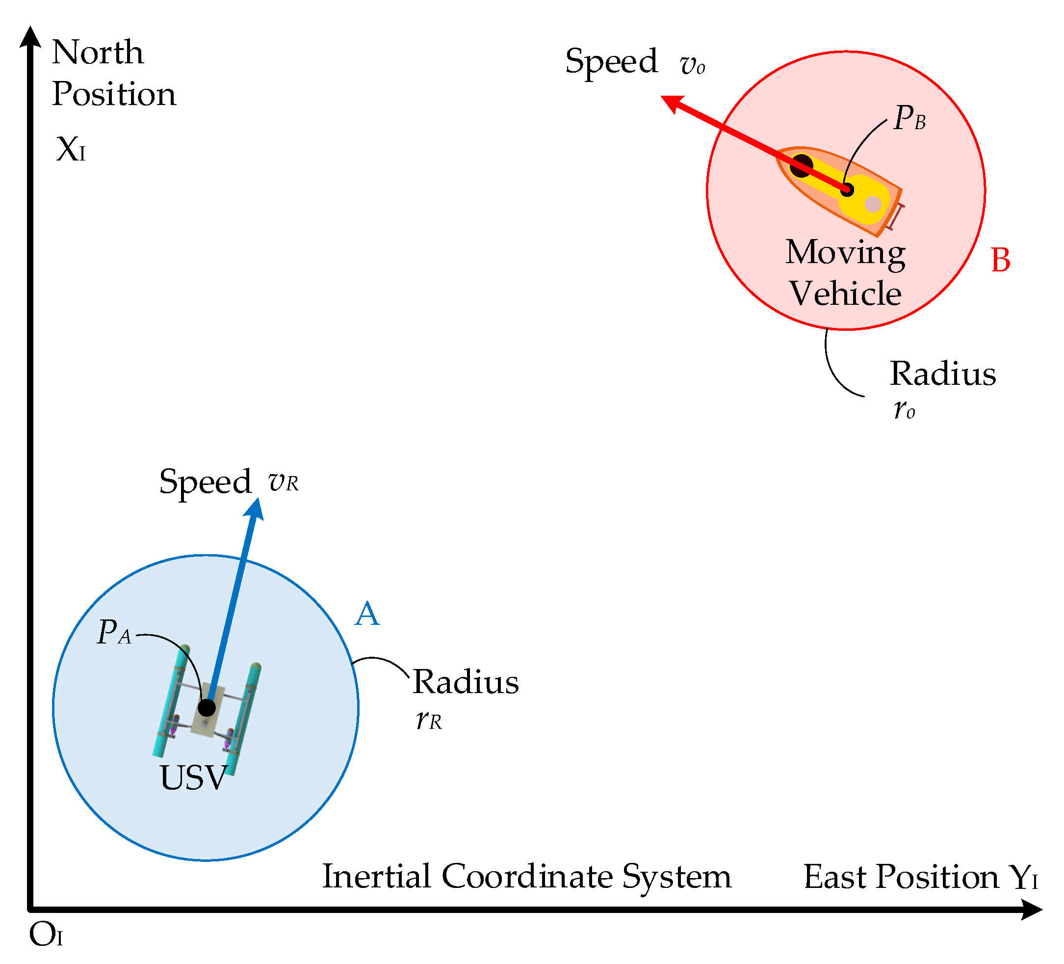
As shown in Figure 1, let A and B denote the circle configuration space with their centers and fixed at the middle of USV and the moving vehicle, respectively. The configuration radii of A and B are depicted by and , and the velocity vectors are represented by and , respectively. The bearing angle between the relative speed and position vector is written as
Hence, the DCPA and TCPA can be calculated as
where DCPA provides the direct collision probability. indicates that a collision is inevitable if two vehicles do not take any avoiding actions. Here, can be set to . When , there exists a possibility of collision. Here, is the preset secure collision-avoidance distance, and it can be set to several times that of . This means that the vehicle must take avoiding actions when . TCPA provides the potential collision probability. A larger TCPA indicates a lower collision probability. The negative TCPA with demonstrates that two vehicles are moving away from each other. To avoid a singularity of TCPA, a small minimum value can be set for .
The direct collision probability based on DCPA can be calculated as
where
The potential collision probability based on TCPA can be calculated as
The comprehensive collision probability can be designed as a combination of the direct collision probability and the potential collision probability, which gives
where and denote the corresponding weights.
3. TVO-Based Collision Avoidance
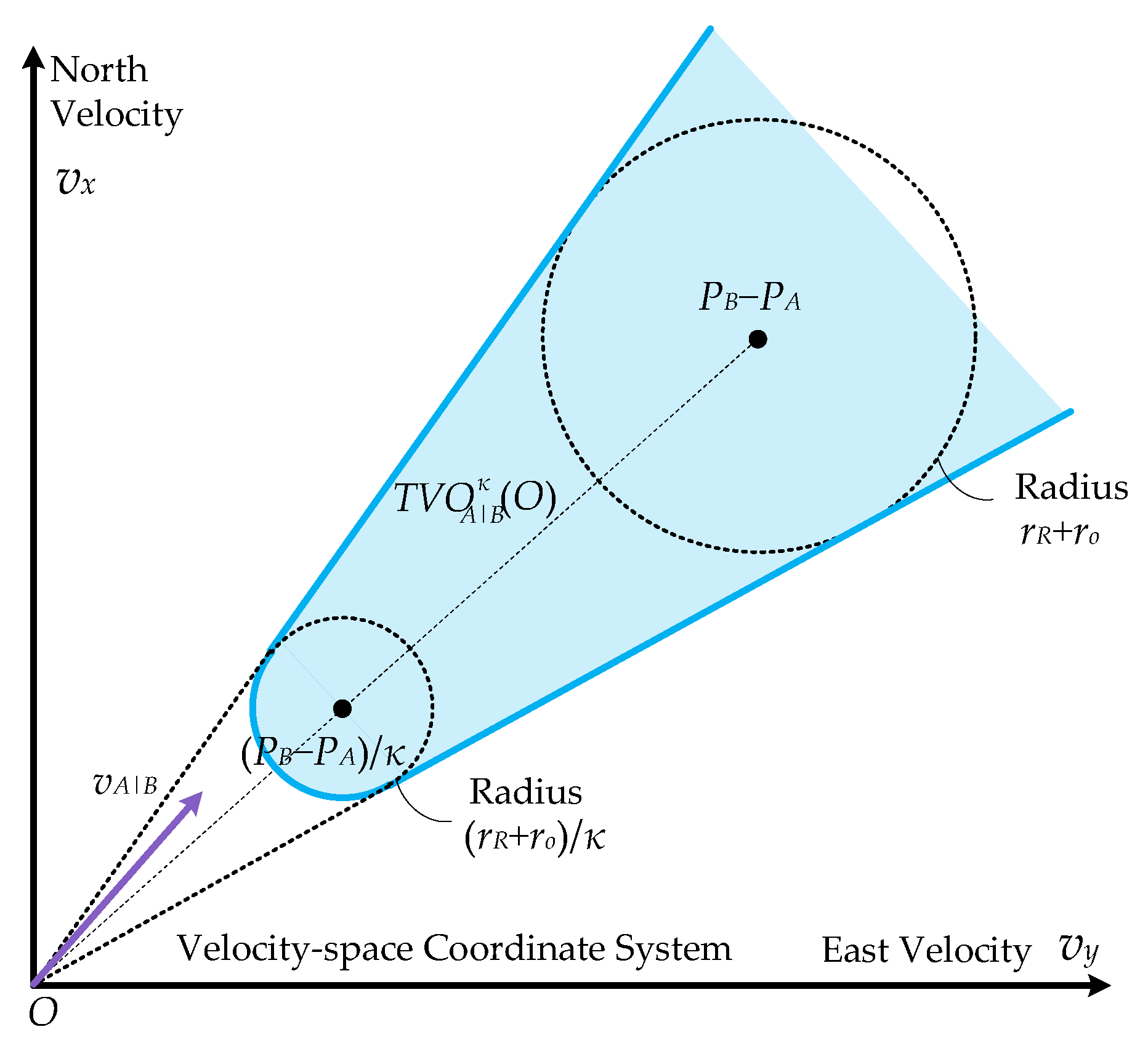
In a velocity space, as shown in Figure 2, let denote an open disc of radius centered at , which gives
According to [38], the TVO with its apex at the origin O of the velocity-space coordinate system is defined as
where is a preset collision-free time period associated with a small . If , a collision between two vehicles will occur at some moment before time , and vice versa. The conventional VO algorithm usually adopts zero time to collision (). This means the vehicle needs to immediately take avoiding actions once the VO algorithm is carried out. Sometimes, we do not expect to take avoiding actions when the distance between two vehicles is far enough away. Hence, a nonzero can be set to truncate the VO.
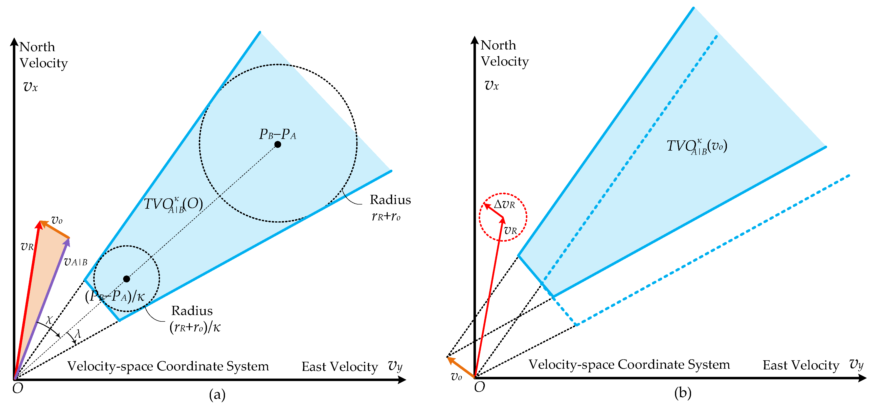
To avoid a collision between these two vehicles, as shown in Figure 3a, it follows that
where represents the change in the aforementioned bearing angle, and is the half cone angle. As shown in Figure 3b, a new TVO is defined by shifting the TVO in Figure 3a from its origin to the apex of the velocity of vehicle B. Notice that the arc boundary of in Figure 3a,b is simplified as a straight line. Given that the collision-free time along this line has a relatively small change, this approximation can facilitate the determination of USV velocity to avoid a collision.
4. Obstacle Expansion Induced by Motion Uncertainties and COLREGS Rules
4.1. COLREGS Rules
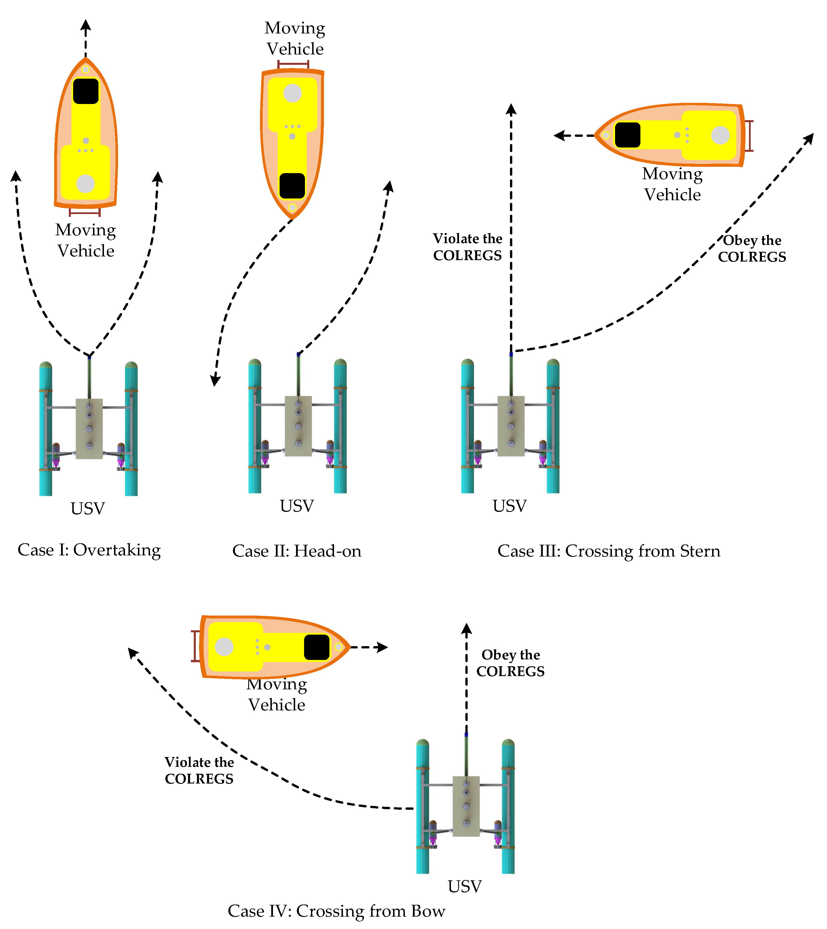
As shown in Figure 4, this paper will discuss three scenarios regulated by the COLREGS rules, i.e., overtaking, head-on, and crossing.
- Overtaking: The own ship should be taken as an overtaking ship when it comes up with another ship from a direction more than 22.5 degrees abaft its beam. The own ship can pass the moving ship on its port side or the starboard side.
- Head-on: When two head-on ships encounter each other on the reciprocal or nearly reciprocal courses, they should alter their courses to starboard such that each should pass on the port side of the other.
- Crossing: When two ships are crossing and have a collision risk, the ship with the other on its own starboard side should keep out of the way and shall, if the circumstances of the case admit, avoid crossing ahead of the other ship.
In Case IV of Figure 4, the COLREGS crossing rule requires that the moving vehicle should keep out of the way to avoid the USV. Considering that some commercial ships with larger sizes have insufficient maneuvering capabilities to actively avoid a USV with a small size, the USV should have a sense of confidence to determine whether to obey or violate the COLREGS rules in an emergency.
4.2. Obstacle Expansion Encouraged by COLREGS
To enhance the operating safety, we suggest that a velocity expansion of the moving vehicle can be designed as a monotone increasing function of the comprehensive collision probability, as shown in Figure 5. As depicted by Case III in Figure 4, the USV is encouraged to obey the COLREGS crossing rule from the stern of the target ship. Therefore, the following adaptive expansion strategy is developed to determine the expansion of the moving ship’s velocity
where denotes the maximum expansion of velocity magnitude, and dominates the decreasing rate. It is worth noting that the above expansion strategy (12) is not unique, and readers can design other kinds of reasonable adaptive laws to replace (12).
As depicted in Figure 5, therefore, a moving vehicle’s velocity considering the measurement uncertainty is formulated within the following range:
where is the parameter that considers the measurement uncertainty of the moving ship’s velocity .
To enhance the operating safety of Cases I and II in Figure 4, the expansion direction of the moving ship’s velocity is chosen to be clockwise. This means that the USV is encouraged to pass from the port side of the moving vehicle instead of its starboard side, which has a good agreement with COLREGS rules. An adaptive direction expansion of velocity is developed as
where b denotes a preset maximum bearing angle that is used to distinguish whether to enter a crossing scenario or not. represents the direction expansion of . is an introduced scaling gain. is a preset minimum value of the relative speed . demonstrates that the USV and the moving ship have almost the same velocity, i.e., . If the collision risk is high with , indicates that a larger direction expansion is generated, which does not encourage the USV to accompany the moving ship on its starboard side. For the overtaking and head-on scenarios, i.e., and , a fixed direction expansion is produced to encourage the USV to take a passing course from the port side of the moving ship. When two vehicles are moving away from each other, i.e., and , no direction expansion is needed.
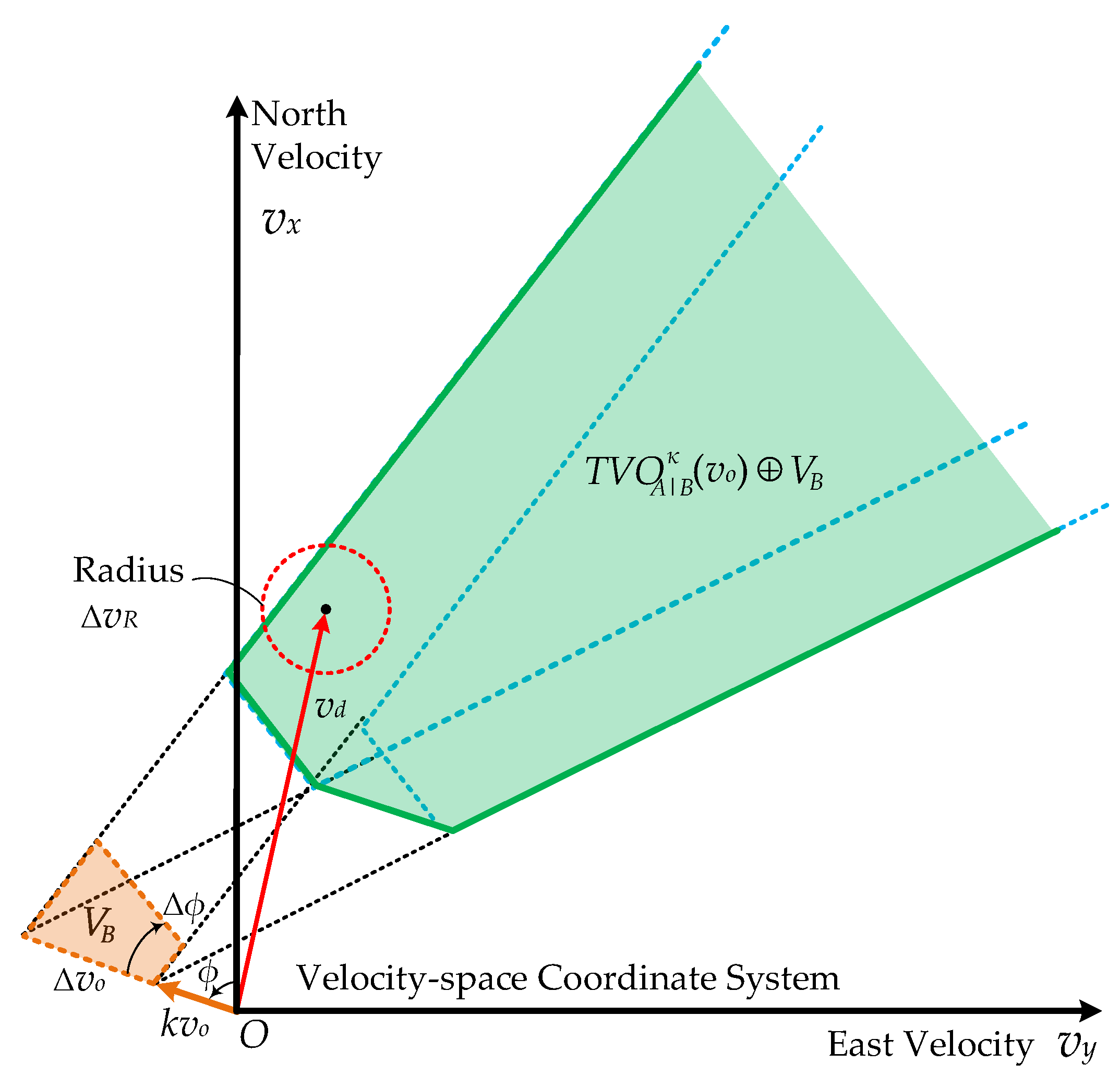
As shown in Figure 5, an adaptive expansion of velocity is formed as a set . By using the Minkowski sum operation between and , a new truncated velocity obstacle is established. Notice that the vehicle’s desired speed vector is generated online by the USV’s guidance system, and a minimum bias speed can be accordingly determined to avoid the velocity obstacle . Thus, the USV’s collision-free velocity is calculated as
which will be sent to the USV’s control system for realization. Detailed assignment for the desired speed is given in Section 5.
5. USV Control System Design
5.1. Mathematical Model for Marine Surface Vessels
Without considering the pitch, roll, and heave motions [42], a three-degree-of-freedom nonlinear model for marine surface vessels can be described as
where vector contains the north position x, east position y, and yaw heading in the inertial coordinate system; vector includes the surge velocity u, sway velocity , and yaw angular velocity r in the body-fixed coordinate system. Rotation matrix is expressed as
nonlinear term provides the Coriolis and centripetal surge and sway forces as well as yaw moment; mass matrix includes the rigid-body mass and the hydrodynamic added mass; nonlinear damping term covers the hydrodynamic damping force and moment; vector is the control input; vector contains the incremental disturbances. The formulations of these matrices can be found in [42,43].
Given that most USVs are underactuated, the sway motion cannot be directly controlled. In this context, expanding from (17) yields the following surge and yaw dynamic models
where and represent the surge mass and the yaw inertial moment, respectively. Nonlinear terms and lump all uncertainties together [44].
5.2. Desired Surge Speed and Yaw Heading Assignment
To accomplish multiple marine tasks, including path following, trajectory tracking, and formation control, the USV is required to follow a predefined trajectory or track a moving target that moves on the predefined trajectory [45,46,47,48,49,50,51]. This predefined trajectory is formed by several waypoints, and each segment can be formulated by a high-order polynomial as the function of a path parameter . Index j represents the jth segment. When and , the USV arrives at the first waypoint and the final waypoint, respectively. Detailed path formulation can be found in [45,49]. As shown in Figure 6, a right-hand moving coordinate system is established with its axis tangent to the path. Its origin moves along this trajectory and an optimal path parameter exists such that its axis can pass through the origin of the USV body-fixed coordinate system [49,52]. To obtain this optimal path parameter , numerical solutions or iteration mechanism methods can be adopted to figure it out. For the numerical solutions, readers can refer to [52]. For the iteration mechanism methods, detailed implementation processes and their summaries can be found in Section III of the research work [49]. To assign a desired yaw heading for the vehicle to track the trajectory, a line-of-sight (LOS) guidance system presented is presented as follows:
where denotes the rotated angle of the moving coordinate system; is the cross-track error; and represents the look-ahead distance.
Here, we do not consider the sideslip effect since the sideslip angle is relatively small in practice (typically lower than 5 degrees) [47,53]. Without considering collision avoidance, therefore, the desired speed vector in Equation (15) can be appropriately assigned as
where is a predefined surge velocity.
Then, the aforementioned collision-avoidance method in Section 4 is used to provide a collision-free vehicle speed , which yields
where and are the collision-free surge velocity and yaw heading, respectively. These two collision-free states act as reference inputs for the control system to realize, which will be presented in Section 5.4.
5.3. State Estimation by Using a Three-Order Differentiator
After obtaining a measured state signal by an onboard sensor or a desired state signal by the above guidance system, here denoted as , their higher-order derivatives are usually indispensable to the control system design. Generally, we can develop a filtering system or use a high-order differentiator to provide these higher-order states for the control implementation [54]. Some typical high-order differentiator designs can be found in [55,56,57,58,59,60]. Here, a three-order differentiator presented in [59] is introduced to provide the USV’s high-order states. Its discrete formulations can be expressed as follows:
where and . The sampling time is defined as . Notice that denotes an index of the present sampling time period . Hence, in this paper, and (if any) describe the corresponding information in the last and next sampling time periods. These three positive gains , , and should be selected to fulfill the Hurwitz requirement associated with a polynomial . As a consequence, , , and here are the filtered position, velocity, and acceleration, respectively.
5.4. SPAE Controller Design
In kinematics, the variations in position and velocity are not independent, and they are naturally produced via the integral process of acceleration. If the variations of position and velocity are constrained by a planned polynomial, the system’s convergence depends solely on the execution of the planned acceleration (the second-order derivative of the planned polynomial) [61]. In this subsection, the proposed SPAE controller consists of three parts: a planned polynomial to satisfy state constraints, an efficient estimation of uncertainty, and an algebraic control law design to carry out the planned acceleration. Notice that the proposed control framework is a digital implementation, which is widely adopted in practical applications.
Let and represent the surge velocity-track error and the yaw heading-track error, respectively. To generate the aforementioned planned accelerations for surge and yaw motions, two state-constrained online polynomial planning strategies are proposed as follows:
- First-order polynomial planning for surge velocity-track motion: for a given time period , a first-order polynomial can be uniquely determined by satisfying the speed-track constraints of the present velocity-track error at time and a zero velocity-track error at time . To execute the acceleration-track error by using the planned acceleration as a reference, i.e., , the surge acceleration can be planned aswhere is the planned surge acceleration for the surge control execution. The collision-free acceleration can be obtained by using the above differentiator with as the input.
- Third-order polynomial planning for yaw heading-track motion: for a given time period , a third-order polynomial planning can be uniquely determined by satisfying the yaw-track constraints of the present states at time and zero states at time . Here, can be assigned as the planned angular acceleration. To execute the angular acceleration-track error by using the planned angular acceleration as a reference, i.e., , the angular acceleration can be planned aswhere is the planned angular acceleration for the yaw control execution. Similarly, the collision-free angular acceleration can be obtained by using the above differentiator with as the input.
To accurately execute the planned surge acceleration (26) and the yaw angular acceleration (27), the discrete velocity-track and yaw-track control laws are presented as follows:
where and are the estimated mass and inertial moment, respectively. It is worth noting that the proposed control laws adopt the estimated uncertainty terms and in the last sampling time period since and have not been updated in the present sampling time period. Therefore, and will be updated for the control executions and in the next sampling time period.
By substituting the control laws (28) and (29) into the discrete dynamic equations of (18) and (19), respectively, the uncertainty terms used for the control executions and in the next sampling time period can be updated as
where and are two introduced positive gains. The feedback angular accelerations can also be obtained by using the above differentiator with the yaw measurement as the input. According to the USV kinematic Equation (16), the feedback surge accelerations can be obtained based on the filtered and .
5.5. System Convergence Analysis
5.5.1. Surge Velocity-Track Convergence
Considering that , substituting the control law (28) and the planned acceleration (26) into the discrete dynamic model of (18) gives
where is defined as a scale factor for the surge mass.
In the next sampling time period, we have
Considering that and , subtracting Equation (32) from Equation (33) yields
where contains the offsets of uncertainties and collision-avoidance acceleration in two nearby sampling time periods. With the decrease in the sampling loop period , the surge uncertainty error will gradually approach zero since and . Therefore, it is clear that the speed-track error system (34) converges in a finite time period.
5.5.2. Yaw Heading-Track Convergence
Considering that , substituting the yaw control law (29) and the planned angular acceleration (27) into the discrete model of (19) gives
where is defined as a scale factor for the yaw inertial moment.
Similarly, we have
where the yaw uncertainty error is defined as . If and , it is also not difficult to validate the convergence of the error system (36) since its left-hand formulation satisfies the Routh–Hurwitz criterion.
6. Main Results and Discussions
6.1. System Setup
The vehicle model used in simulations is an underactuated USV powered by two fixed thrusters at the stern. The inertial mass of this vehicle is 40 kg. Its inertial moment is 12.8 . Detailed descriptions of this USV can be found in [10,44,62]. Implementation processes of the proposed methods are summarized in a block diagram, as shown in Figure 7. Based on a number of simulations, the preset parameters for simulated validations were fine-tuned and are listed in Table 1.
6.2. USV Passive Collision Avoidance
This subsection presents the main results of the passive collision-avoidance scenario where only the USV takes action to avoid collision with other moving vehicles. All the vehicles are represented by configuration circles, and the graphical representation of each circle was recorded every 8 s with a gradient color. The initial configuration circles for all the vehicles are marked in red. When the USV arrives at the goal, the USV, vehicle B, vehicle C, and vehicle D are marked in blue, black, pink, and cyan, respectively.
Firstly, the head-on and overtaking scenarios were selected for simulated validations. As shown in the first plot of Figure 8, both the USV and the moving vehicle B were initially heading toward each other. After about 32 s, the USV altered its heading to the port side of vehicle B to avoid a collision, which obeys the COLREGS head-on rule. After 48 s, the USV returned to its initial path. As shown in the second and third plots of Figure 8, there are two different collision-avoidance actions when the USV overtook vehicle B. The USV speed was 0.5 m/s, and the speed of vehicle B was 0.16 m/s. The initial position of vehicle B was (0 m, 18 m), and the initial positions of USV were (−2 m, −15 m) and (−2 m, −5 m), respectively. When the USV was far away from vehicle B in the overtaking scenario (second plot), Equation (14) indicates that the clockwise orientation expansion of vehicle B was larger, thereby resulting in the overtaking on the port side of vehicle B. In the third plot, the USV had a sense of confidence to pass vehicle B’s starboard side. Notice that both overtaking actions obey the COLREGS rules.
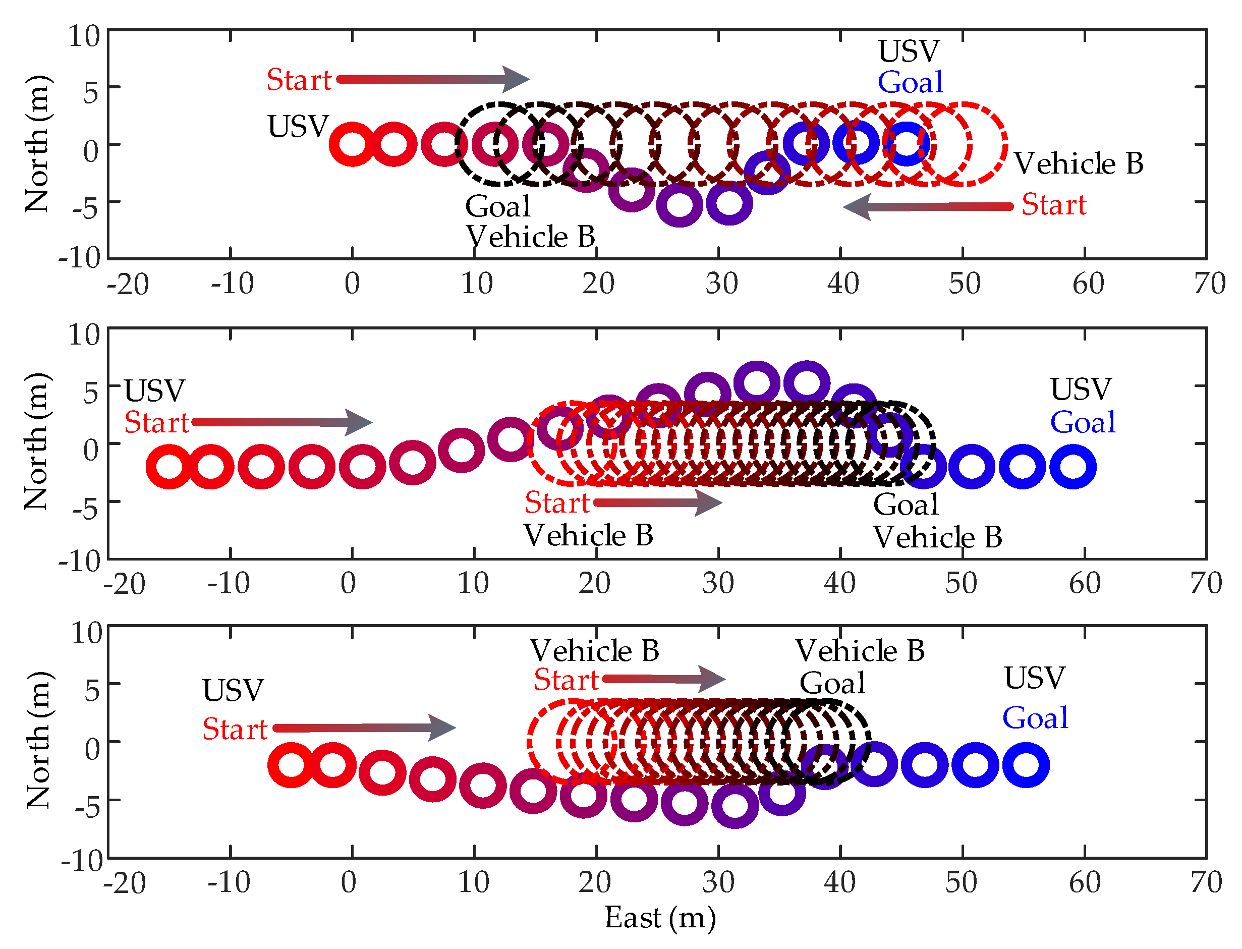
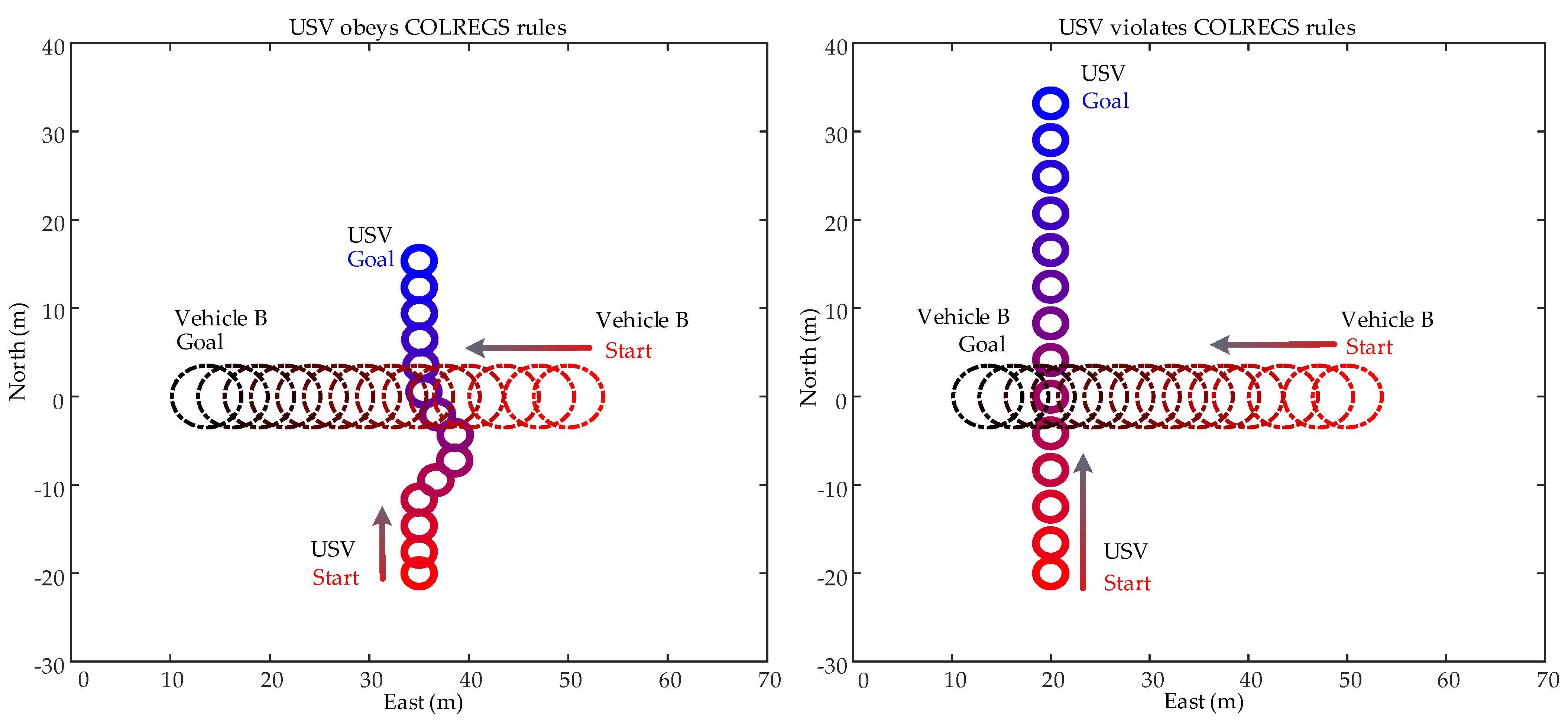
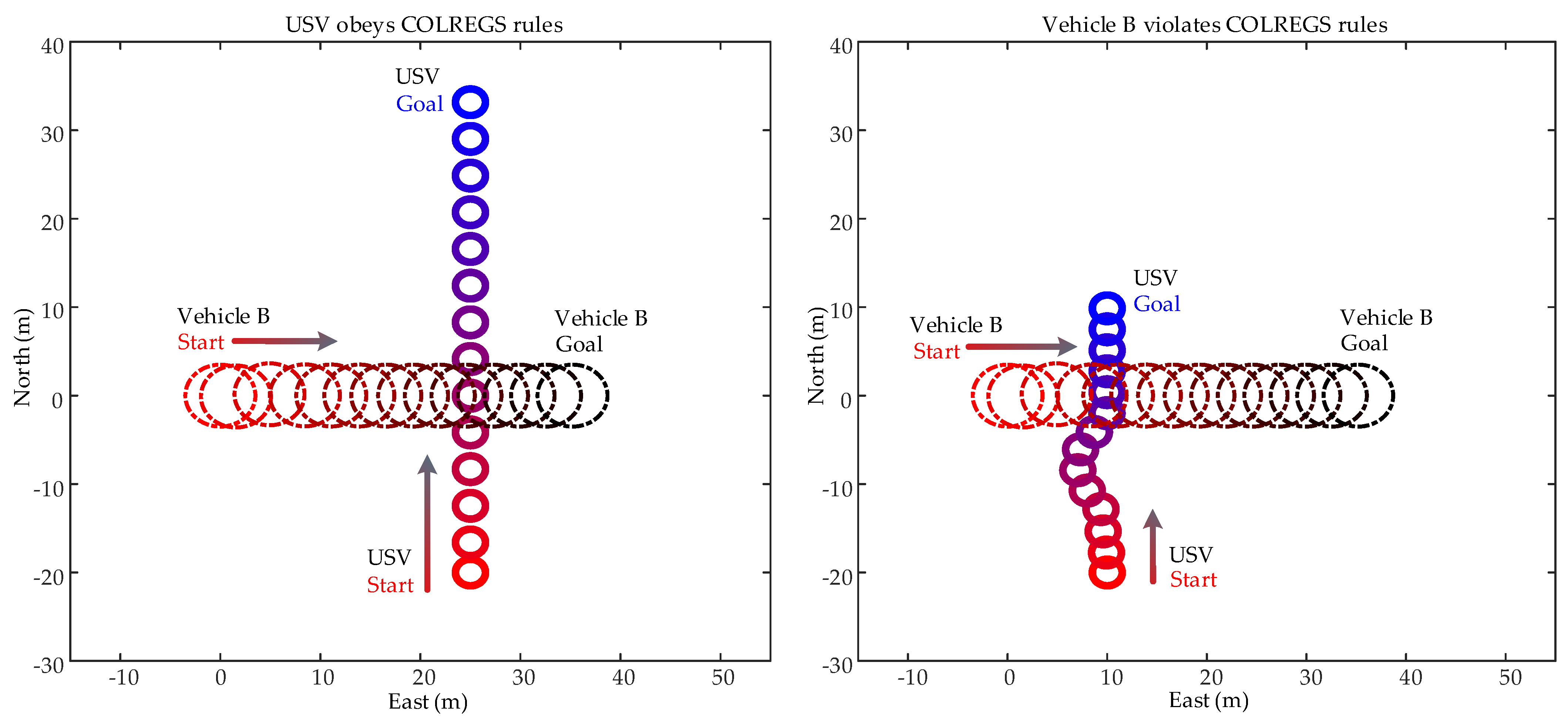
Secondly, different crossing scenarios were selected for simulated validations. As shown in Figure 9, the USV had the moving vehicle B on its own starboard side when the simulations started. Vehicle B started at position (0 m, 50 m) with a constant speed of 0.33 m/s. In the first plot of Figure 9, the USV started at position (−20 m, 35 m) with a lower speed of 0.37 m/s, and it took a collision-avoidance path from vehicle B’s stern, which obeys the COLREGS crossing rule. However, when the USV was far away from vehicle B and had a larger speed of 0.5 m/s, as shown in the second plot of Figure 9, it directly took the crossing action from vehicle B’s bow, which violated the COLREGS crossing rule. As shown in Figure 10, the USV had the moving vehicle B on its own port side when the simulations started. The difference is that vehicle B violated the COLREGS crossing rule in this case, which is expected to occur in reality. It can be observed that this situation can also be safely handled.
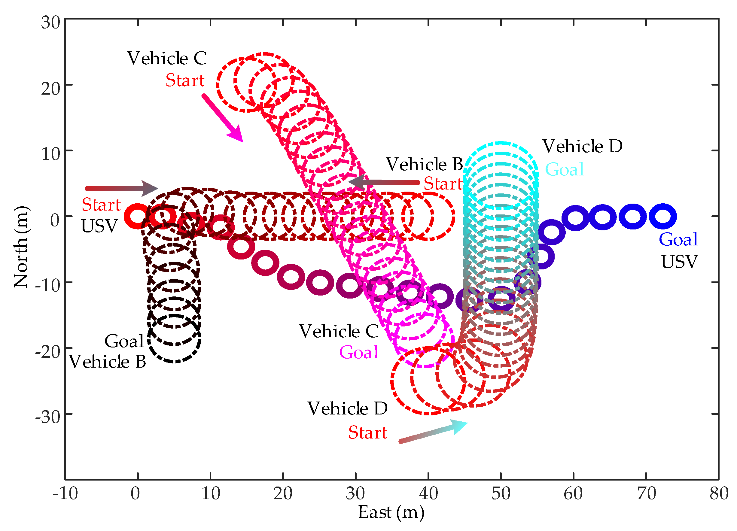
Then, the collision-avoidance scenarios with multiple vehicles were selected for simulated validations. As shown in Figure 11, the USV, vehicle B, vehicle C, and vehicle D started at positions (0 m, 0 m), (40 m, 0 m), (20 m, 15 m), and (−25 m, 40 m), respectively. At the beginning, there was a head-on situation between the USV and vehicle B. Then, the USV successfully took the crossing route from the bow of vehicle C and the stern of vehicle D one by one. It can be observed that the proposed real-time collision-avoidance method provided a reasonable balance between safety and compliance with COLREGS rules and had remarkable performances in passively avoiding other vehicles.
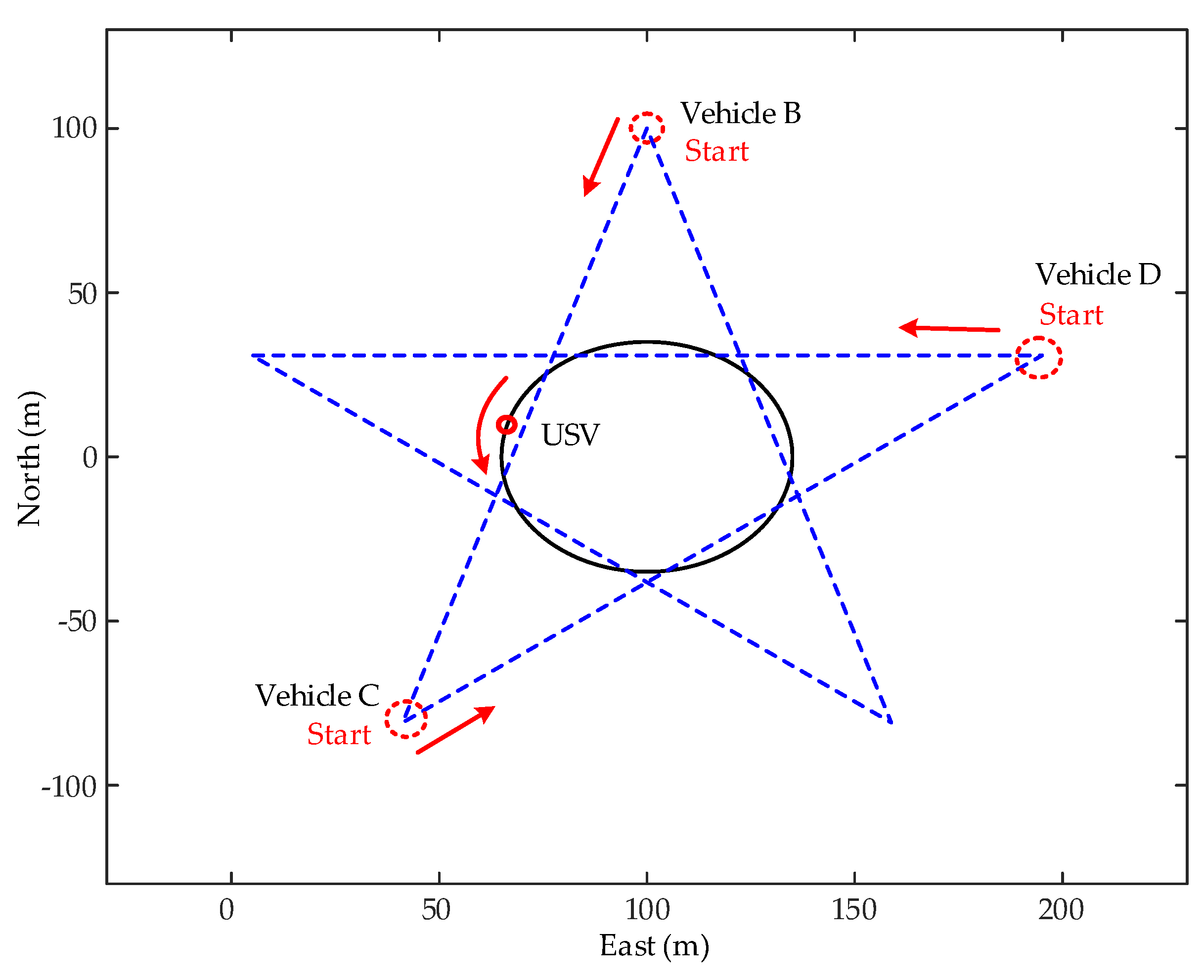
For comparative purposes, finally, the passive collision-avoidance scenario in Figure 12 was carried out. The closed-loop trajectories for Vehicles B, C, and D were the edges of a five-pointed star, and these vehicles started their positions from three different apexes. In particular, the velocities of Vehicles B, C, and D were set to time-varying sinusoidal functions with the same average speed of 0.5 m/s, the same period, and different phase angles. The USV moved along a circular trajectory in an anti-clockwise direction with a constant speed of 0.5 m/s. Comparisons among different methods were made and are listed in Table 2. We can observe that the USV with our proposed method successfully avoided all the obstacles. Instead of blindly obeying the COLREGS rules, the proposed method may violate these rules to safely and successfully avoid other vehicles compared to the other two methods.
6.3. Active Collision Avoidance among Multiple Vehicles
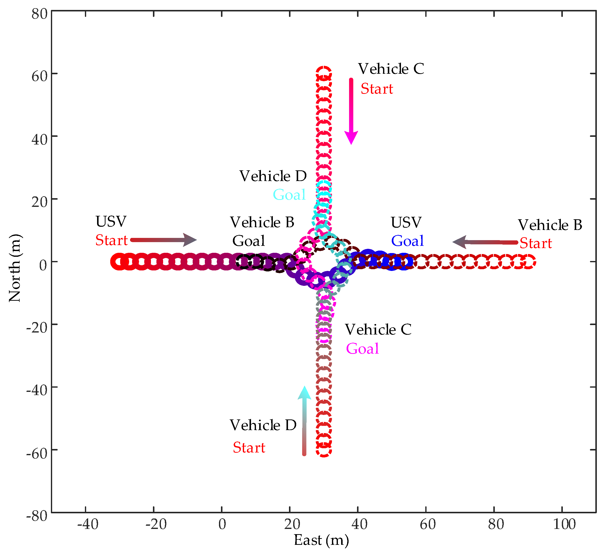
Unlike the aforementioned passive collision avoidance, the active situation allows other vehicles to adopt the same collision-avoidance method. The main results of active collision avoidance are presented in this subsection. The configuration radii for all the vehicles were set to 2 m. As shown in Figure 13, four vehicles started to move towards the same position (0 m, 30 m) from four different directions. It can be observed that these vehicles simultaneously altered their headings to the starboard side to avoid a collision, which is quite similar to entering and exiting the roundabout at the same time. As shown in Figure 14, the USV, vehicle B, vehicle C, and vehicle D started their positions at (0 m, 0 m), (40 m, 0 m), (20 m, 15 m), and (−25 m, 40 m), respectively. At the beginning, there was a head-on situation between the USV and vehicle B. Unlike the complex scenarios presented in Figure 12, it was safer when all vehicles took collision-avoidance actions. Moreover, the USV successfully took the crossing route from the bow of vehicle D, which violated the crossing rule of COLREGS. The main results of active collision avoidance also provide a reasonable balance between safety and compliance with COLREGS rules.
6.4. Simulated and Experimental Validations of the Proposed SPAE Controller
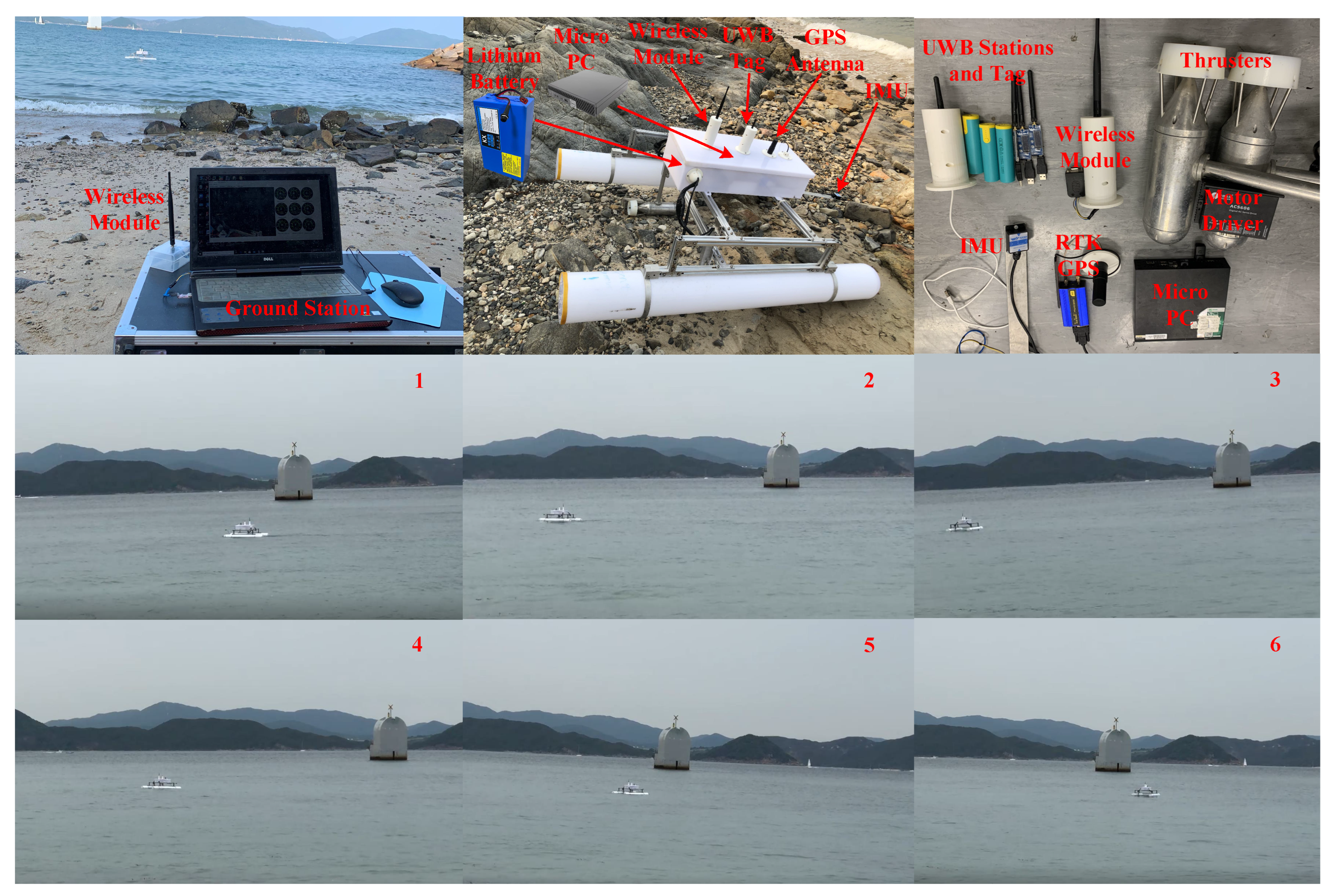
To validate the proposed SPAE controller experimentally, the passive crossing scenario shown in Figure 10 was selected as a collision-avoidance example and carried out to provide the collision-free desired heading and surge speed for the proposed controller to realize. The experiments were conducted at the offshore seaside of Hong Kong University of Science and Technology (HKUST), as shown in Figure 15. The experimental collision-free desired heading and surge speed were adopted for the simulated validations of the proposed SPAE controller. In particular, the nonlinear positioning control method presented in [44] was conducted to provide the estimated time-varying environmental disturbances that were considered in the simulations.
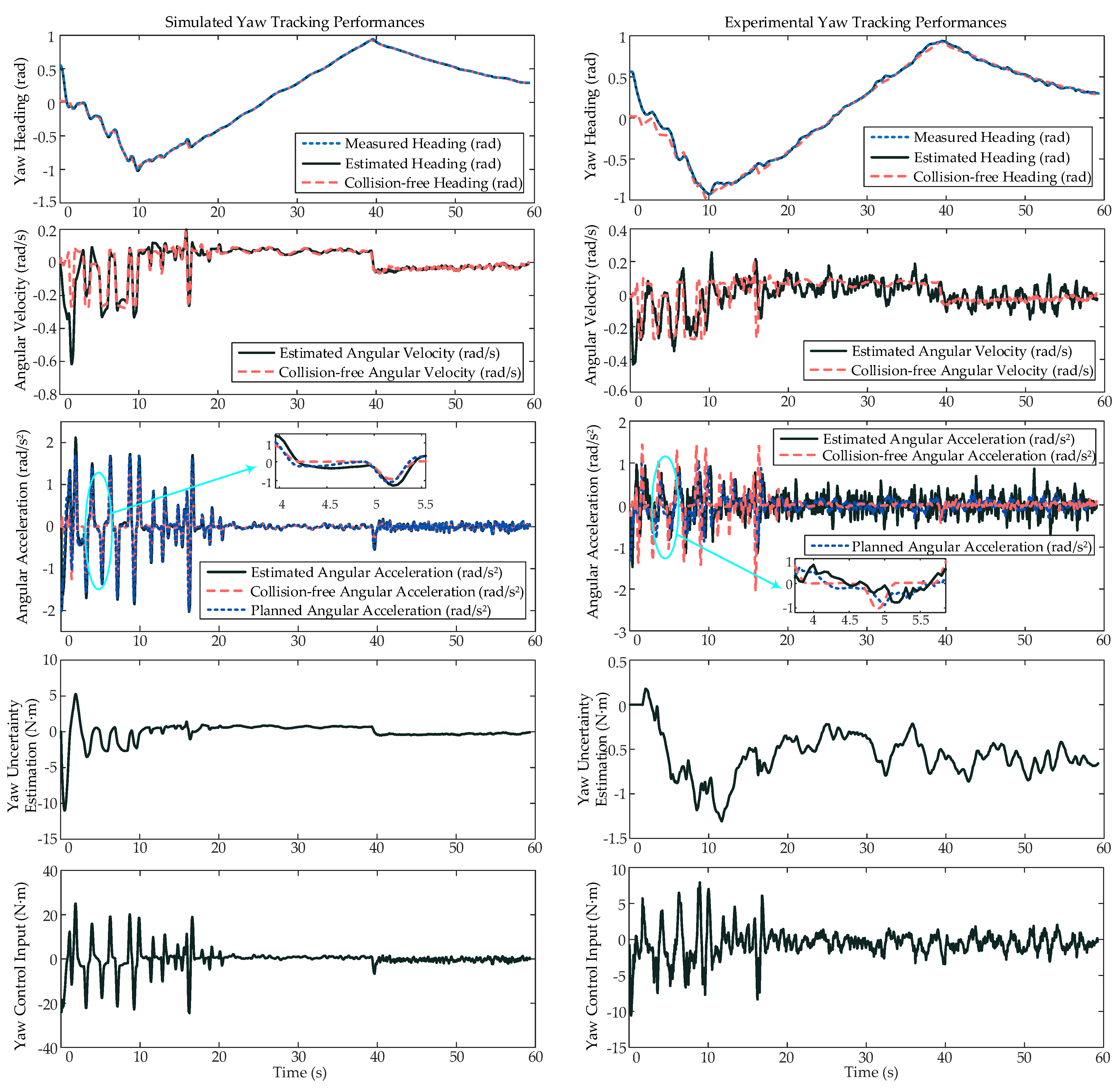
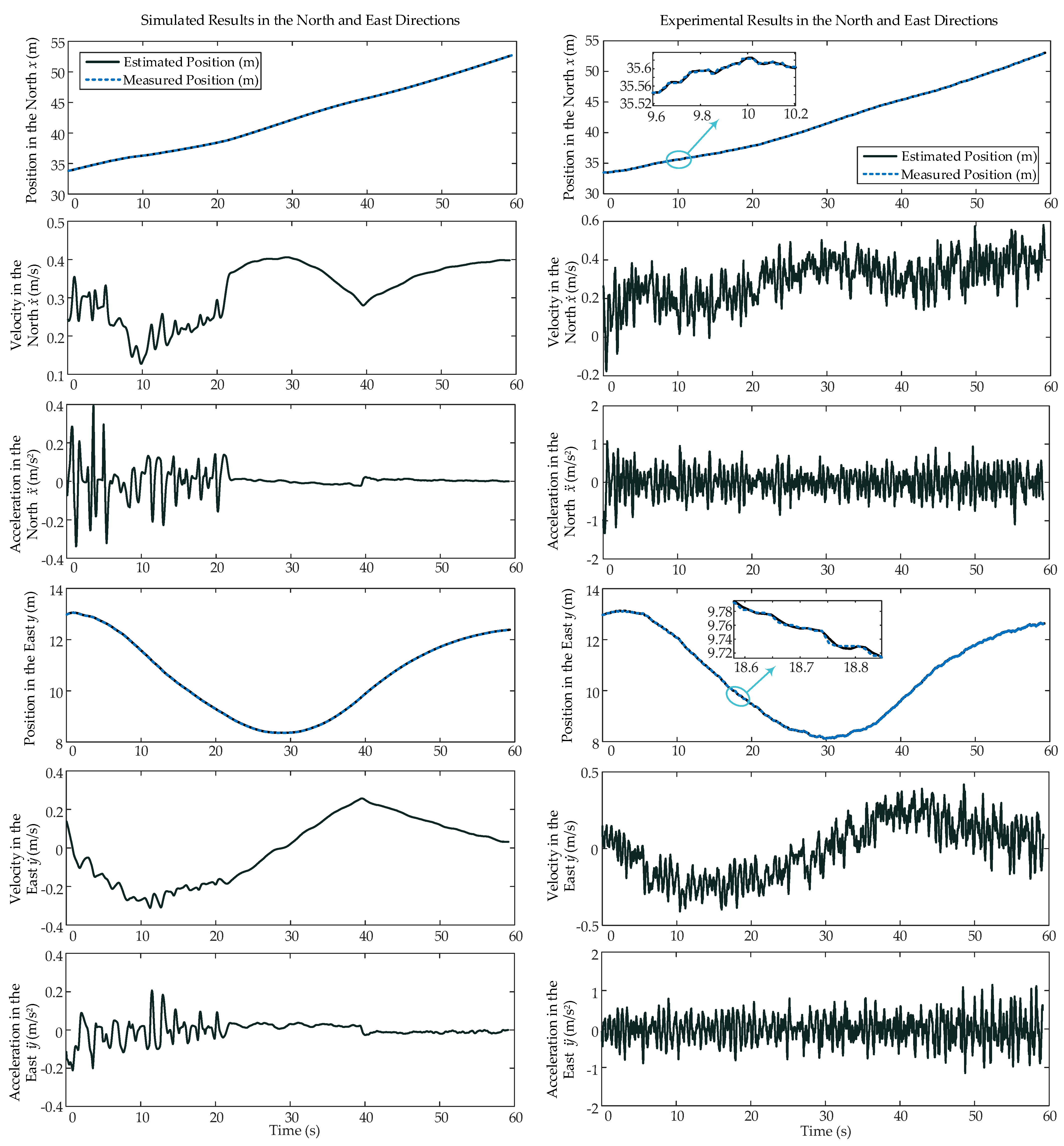
The simulated and experimental plane motions are shown in Figure 16. In this case, a virtual moving vehicle was created on the ocean surface. It had a constant moving forward speed of 0.4 m/s and came from the USV’s port side. The experimental horizontal trajectory demonstrated that the USV took a collision-avoidance action from the moving vehicle’s stern. The yaw-track heading errors and surge-track velocity errors are plotted in the right subplots of Figure 16. Simulated and experimental yaw-track results are shown in Figure 17. Before 18 seconds, we can observe that the vehicle yaw heading had chattering responses due to the switches between a potential collision and a collision-free situation. As demonstrated in Figure 5, the decreasing yaw heading indicated that the USV speed was within the TVO area such that an anticlockwise yaw rotation was needed to avoid the obstacle. Conversely, the increasing yaw heading indicated that the USV speed was out of the TVO area. Clockwise yaw rotation was taken to move closer to the preset path-following trajectory. The yaw-track heading error and its angular velocity error were used to calculate the planned angular acceleration (blue dashed line). The yaw uncertainty term was estimated by using the planned angular acceleration and the feedback-estimated angular acceleration (black solid line). With the yaw control inputs, we can observe that the feedback-estimated angular acceleration , the planned angular acceleration , and the collision-free angular acceleration (black solid line) had a good agreement with each other, especially in simulations. The north-east state estimations presented in Figure 18 were used to calculate the surge velocity and acceleration on the basis of USV’s kinematic Equation (16). In Figure 19, similarly, the surge-track velocity error was adopted to calculate the planned surge acceleration (blue dashed line). We can also observe that the feedback-estimated surge acceleration , the planned acceleration , and the collision-free acceleration (black solid line) had a good agreement with each other, especially in simulations. Overall, accurate yaw-track and surge-track control performances were obtained by using the proposed controller since system lower-order states are actually the integration of the system’s acceleration.
7. Conclusions
Firstly, this paper has developed an emergency collision-avoidance method for unmanned surface vehicles with the COLREGS rules flexibly obeyed. The proposed collision-avoidance method inherits the real-time reaction characteristics of the velocity obstacle (TVO) algorithm. Its main feature is to greatly encourage the USV to follow the COLREGS rules based on an expansion of a truncated velocity obstacle (TVO). From a security standpoint, it is not mandatory for the USV to obey the COLREGS rules when it has a high collision risk with other ships. With only the velocity uncertainty of the target ship considered in the VTO’s expansion, uniform collision avoidance tasks can be carried out regardless of the emergency level. In sum, the proposed algorithm can efficiently handle multiple obstacles by providing quantitative solutions in different scenarios, including passive and active avoiding actions.
With the collision-free yaw heading and surge velocity as an input, secondly, a discrete simultaneous planning and executing (SPAE) controller has been developed to promptly realize these assigned objectives. All selected error state constraints are satisfied via an online planned polynomial so that a planned acceleration can be promptly generated for control execution. Based on a well-estimated uncertainty term, the control law that is formulated as an algebraic formulation can accurately execute the system acceleration to track the planned acceleration, which ensures tracking performance. Only a control gain is introduced in the controller design, and there is no need to fine-tune this control gain. The developed control framework demonstrates that it is easy for readers to understand it and carry it out. The main results have shown remarkable collision-avoidance performance under both passive and active collision-avoidance modes. Both simulations and experiments have been carried out to verify the proposed controller design.
In collision risk assignment, the collision risk index (CRI) was calculated as the linear combination of the DCPS and TCPA according to the research work in this field. However, more factors may affect the calculation of CRI, such as a vehicle’s maneuvering capacity and the reliability of the perception system. For further investigation, it would be interesting to develop a collision-avoidance method that can take into account the maneuvering capacity of USV and the reliability of an onboard perception system.
Author Contributions
Conceptualization, Y.Q. and L.C.; methodology, Y.Q. and L.C.; software, Y.Q.; validation, Y.Q.; data curation, Y.Q.; writing—original draft preparation, Y.Q.; writing—review and editing, Y.Q. and L.C.; supervision, L.C.; project administration, L.C. All authors have read and agreed to the published version of the manuscript.
Funding
The research work was supported by the Research Grants Council of Hong Kong under project no. 16205919.
Institutional Review Board Statement
Not applicable.
Informed Consent Statement
Not applicable.
Data Availability Statement
Not applicable.
Acknowledgments
The authors would like to thank the editors and all reviewers for the comments and suggestions to improve the quality of this article.
Conflicts of Interest
The authors declare no conflict of interest.
References
- Campbell, S.; Naeem, W.; Irwin, G.W. A review on improving the autonomy of unmanned surface vehicles through intelligent collision avoidance manoeuvres. Annu. Rev. Control 2012, 36, 267–283. [Google Scholar] [CrossRef] [Green Version]
- Liu, Z.; Zhang, Y.; Yu, X.; Yuan, C. Unmanned surface vehicles: An overview of developments and challenges. Annu. Rev. Control 2016, 41, 71–93. [Google Scholar] [CrossRef]
- Qu, Y.; Xu, H.; Yu, W.; Feng, H.; Han, X. Inverse optimal control for speed-varying path following of marine vessels with actuator dynamics. J. Mar. Sci. Appl. 2017, 16, 225–236. [Google Scholar] [CrossRef]
- Vu, M.T.; Choi, H.S.; Kim, J.Y.; Tran, N.H. A study on an underwater tracked vehicle with a ladder trencher. Ocean Eng. 2016, 127, 90–102. [Google Scholar] [CrossRef]
- Vu, M.T.; Choi, H.S.; Nguyen, N.D.; Kim, S.K. Analytical design of an underwater construction robot on the slope with an up-cutting mode operation of a cutter bar. Appl. Ocean Res. 2019, 86, 289–309. [Google Scholar] [CrossRef]
- Zhang, W.; Shen, P.; Qi, H.; Zhang, Q.; Ma, T.; Li, Y. AUV path planning algorithm for terrain aided navigation. J. Mar. Sci. Eng. 2022, 10, 1393. [Google Scholar] [CrossRef]
- Zeng, X.; Xia, M.; Luo, Z.; Shang, J.; Xu, Y.; Yin, Q. Design and control of an Underwater Robot Based on Hybrid Propulsion of Quadrotor and Bionic Undulating Fin. J. Mar. Sci. Eng. 2022, 10, 1327. [Google Scholar] [CrossRef]
- Zhu, M.; Sun, W.; Wen, Y.; Huang, L. Extended state observer-based parameter identification of response model for autonomous vessels. J. Mar. Sci. Eng. 2022, 10, 1291. [Google Scholar] [CrossRef]
- Peng, Z.; Wang, D.; Chen, Z.; Hu, X.; Lan, W. Adaptive dynamic surface control for formations of autonomous surface vehicles with uncertain dynamics. IEEE Trans. Control Syst. Technol. 2012, 21, 513–520. [Google Scholar] [CrossRef]
- Qu, Y.; Cai, L. Nonlinear positioning control for underactuated unmanned surface vehicles in the presence of environmental disturbances. IEEE/ASME Trans. Mechatronics 2022, 27, 1–11. [Google Scholar] [CrossRef]
- Sarda, E.I.; Qu, H.; Bertaska, I.R.; von Ellenrieder, K.D. Station-keeping control of an unmanned surface vehicle exposed to current and wind disturbances. Ocean Eng. 2016, 127, 305–324. [Google Scholar] [CrossRef] [Green Version]
- Caceres-Cruz, J.; Arias, P.; Guimarans, D.; Riera, D.; Juan, A.A. Rich vehicle routing problem: Survey. ACM Comput. Surv. 2014, 47, 32. [Google Scholar] [CrossRef]
- Ayawli, B.B.K.; Chellali, R.; Appiah, A.Y.; Kyeremeh, F. An overview of nature-inspired, conventional, and hybrid methods of autonomous vehicle path planning. J. Adv. Transp. 2018, 2018, 8269698. [Google Scholar] [CrossRef]
- Huang, S.; Teo, R.S.H.; Tan, K.K. Collision avoidance of multi unmanned aerial vehicles: A review. Annu. Rev. Control 2019, 48, 147–164. [Google Scholar] [CrossRef]
- Yasin, J.N.; Mohamed, S.A.; Haghbayan, M.H.; Heikkonen, J.; Tenhunen, H.; Plosila, J. Unmanned aerial vehicles (uavs): Collision avoidance systems and approaches. IEEE Access 2020, 8, 105139–105155. [Google Scholar] [CrossRef]
- Ozturk, U.; Cicek, K. Individual collision risk assessment in ship navigation: A systematic literature review. Ocean Eng. 2019, 180, 130–143. [Google Scholar] [CrossRef]
- Huang, Y.; Chen, L.; Chen, P.; Negenborn, R.R.; van Gelder, P.H.A.J.M. Ship collision avoidance methods: State-of-the-art. Saf. Sci. 2020, 121, 451–473. [Google Scholar] [CrossRef]
- Akdağ, M.; Solnør, P.; Johansen, T.A. Collaborative collision avoidance for Maritime Autonomous Surface Ships: A review. Ocean Eng. 2022, 250, 110920. [Google Scholar] [CrossRef]
- Yang, Z.; Li, Y.; Wang, B.; Ding, S.; Jiang, P. A lightweight sea surface object detection network for unmanned surface vehicles. J. Mar. Sci. Eng. 2022, 10, 965. [Google Scholar] [CrossRef]
- Shi, J.; Liu, Z. Track pairs collision detection with applications to ship collision risk assessment. J. Mar. Sci. Eng. 2022, 10, 216. [Google Scholar] [CrossRef]
- Song, L.; Chen, H.; Xiong, W.; Zaopeng, D.; Mao, P.; Xiang, Z.; Hu, K. Method of emergency collision avoidance for unmanned surface vehicle (USV) based on motion ability database. Pol. Marit. Res. 2019, 26, 55–67. [Google Scholar] [CrossRef] [Green Version]
- Li, J.; Zhang, G.; Liu, C.; Zhang, W. COLREGs-constrained adaptive fuzzy event-triggered control for underactuated surface vessels with the actuator failures. IEEE Trans. Fuzzy Syst. 2020, 29, 3822–3832. [Google Scholar] [CrossRef]
- Bakdi, A.; Vanem, E. Fullest COLREGs evaluation using fuzzy logic for collaborative decision-making analysis of autonomous ships in complex situations. IEEE Trans. Intell. Transp. Syst. 2022, 23, 18433–18445. [Google Scholar] [CrossRef]
- Lyu, H.; Yin, Y. COLREGS-constrained real-time path planning for autonomous ships using modified artificial potential fields. J. Navig. 2019, 72, 588–608. [Google Scholar] [CrossRef]
- Zhu, Z.; Lyu, H.; Zhang, J.; Yin, Y. An efficient ship automatic collision avoidance method based on modified artificial potential field. J. Mar. Sci. Eng. 2021, 10, 3. [Google Scholar] [CrossRef]
- Tan, G.; Zhuang, J.; Zou, J.; Wan, L.; Sun, Z. Artificial potential field-based swarm finding of the unmanned surface vehicles in the dynamic ocean environment. Int. J. Adv. Robot. Syst. 2020, 17, 1729881420925309. [Google Scholar] [CrossRef]
- Colito, J. Autonomous mission planning and execution for unmanned surface vehicles in compliance with the marine rules of the road. Master’s Thesis, University of Washington, Seattle, WA, USA, 2007. [Google Scholar]
- Zhao, L.; Roh, M.I. COLREGs-compliant multiship collision avoidance based on deep reinforcement learning. Ocean Eng. 2019, 191, 106436. [Google Scholar] [CrossRef]
- Xu, X.; Cai, P.; Ahmed, Z.; Yellapu, V.S.; Zhang, W. Path planning and dynamic collision avoidance algorithm under COLREGs via deep reinforcement learning. Neurocomputing 2022, 468, 181–197. [Google Scholar] [CrossRef]
- Xu, X.; Lu, Y.; Liu, X.; Zhang, W. Intelligent collision avoidance algorithms for USVs via deep reinforcement learning under COLREGs. Ocean Eng. 2020, 217, 107704. [Google Scholar] [CrossRef]
- Li, L.; Wu, D.; Huang, Y.; Yuan, Z.M. A path planning strategy unified with a COLREGS collision avoidance function based on deep reinforcement learning and artificial potential field. Appl. Ocean Res. 2021, 113, 102759. [Google Scholar] [CrossRef]
- Xu, Q.; Yang, Y.; Zhang, C.; Zhang, L. Deep convolutional neural network-based autonomous marine vehicle maneuver. Int. J. Fuzzy Syst. 2018, 20, 687–699. [Google Scholar] [CrossRef]
- Xie, S.; Garofano, V.; Chu, X.; Negenborn, R.R. Model predictive ship collision avoidance based on Q-learning beetle swarm antenna search and neural networks. Ocean Eng. 2019, 193, 106609. [Google Scholar] [CrossRef]
- Song, A.L.; Su, B.Y.; Dong, C.Z.; Shen, D.W.; Xiang, E.Z.; Mao, F.P. A two-level dynamic obstacle avoidance algorithm for unmanned surface vehicles. Ocean Eng. 2018, 170, 351–360. [Google Scholar] [CrossRef]
- Song, L.; Chen, Z.; Zaopeng, D.; Xiang, Z.; Mao, Y.; Su, Y.; Hu, K. Collision avoidance planning for unmanned surface vehicle based on eccentric expansion. Int. J. Adv. Robot. Syst. 2019, 16, 172988141985194. [Google Scholar] [CrossRef]
- Fiorini, P.; Shiller, Z. Motion planning in dynamic environments using velocity obstacles. Int. J. Robot. Res. 1998, 17, 760–772. [Google Scholar] [CrossRef]
- Snape, J.; Guy, S.J.; Vembar, D.; Lake, A.; Lin, M.C.; Manocha, D. Reciprocal collision avoidance and navigation for video games. In Proceedings of the Game Developers Conference, San Francisco, CA, USA, 5–9 March 2012; Volume 1. [Google Scholar]
- Berg, J.v.d.; Guy, S.J.; Lin, M.; Manocha, D. Reciprocal n-body collision avoidance. In Robotics Research; Springer: Berlin/Heidelberg, Germany, 2011; pp. 3–19. [Google Scholar]
- Kuwata, Y.; Wolf, M.T.; Zarzhitsky, D.; Huntsberger, T.L. Safe maritime autonomous navigation with OLREGS, using velocity obstacles. IEEE J. Ocean. Eng. 2014, 39, 110–119. [Google Scholar] [CrossRef]
- Zhao, Y.; Li, W.; Shi, P. A real-time collision avoidance learning system for unmanned surface vessels. Neurocomputing 2016, 182, 255–266. [Google Scholar] [CrossRef]
- Huang, Y.; Chen, L.; van Gelder, P.H.A.J.M. Generalized velocity obstacle algorithm for preventing ship collisions at sea. Ocean Eng. 2019, 173, 142–156. [Google Scholar] [CrossRef]
- Fossen, T.I. Handbook of Marine Craft Hydrodynamics and Motion Control; John Wiley & Sons: Hoboken, NJ, USA, 2011. [Google Scholar]
- Skjetne, R.; Smogeli, ØN.; Fossen, T.I. A nonlinear ship manoeuvering model: Identification and adaptive control with experiments for a model ship. Model. Identif. Control 2004, 25, 3–27. [Google Scholar] [CrossRef] [Green Version]
- Qu, Y.; Cai, L. Nonlinear station keeping control for underactuated unmanned surface vehicles to resist environmental disturbances. Ocean Eng. 2022, 246, 110603. [Google Scholar] [CrossRef]
- Skjetne, R. The maneuvering problem. Ph.D. Thesis, Norwegian University of Science and Technology, Trondheim, Norway, 2005. [Google Scholar]
- Fossen, T.I.; Pettersen, K.Y. On uniform semiglobal exponential stability (USGES) of proportional line-of-sight guidance laws. Automatica 2014, 50, 2912–2917. [Google Scholar] [CrossRef] [Green Version]
- Fossen, T.I.; Pettersen, K.Y.; Galeazzi, R. Line-of-sight path following for Dubins paths with adaptive sideslip compensation of drift forces. IEEE Trans. Control Syst. Technol. 2015, 23, 820–827. [Google Scholar] [CrossRef] [Green Version]
- Caharija, W.; Pettersen, K.Y.; Bibuli, M.; Calado, P.; Zereik, E.; Braga, J.; Gravdahl, J.T.; Sørensen, A.J.; Milovanović, M.; Bruzzone, G. Integral line-of-sight guidance and control of underactuated marine vehicles: Theory, simulations, and experiments. IEEE Trans. Control Syst. Technol. 2016, 24, 1623–1642. [Google Scholar] [CrossRef] [Green Version]
- Qu, Y.; Cai, L.; Xu, H. Curved path following for unmanned surface vehicles with heading amendment. IEEE Trans. Syst. Man, Cybern. Syst. 2021, 51, 4183–4192. [Google Scholar] [CrossRef]
- Singh, Y.; Sharma, S.; Sutton, R.; Hatton, D.; Khan, A. A constrained A* approach towards optimal path planning for an unmanned surface vehicle in a maritime environment containing dynamic obstacles and ocean currents. Ocean Eng. 2018, 169, 187–201. [Google Scholar] [CrossRef] [Green Version]
- Singh, Y.; Bibuli, M.; Zereik, E.; Sharma, S.; Khan, A.; Sutton, R. A novel double layered hybrid multi-robot framework for guidance and navigation of unmanned surface vehicles in a practical maritime environment. J. Mar. Sci. Eng. 2020, 8, 624. [Google Scholar] [CrossRef]
- Lekkas, A.M.; Fossen, T.I. Integral LOS path following for curved paths based on a monotone cubic hermite spline parametrization. IEEE Trans. Control Syst. Technol. 2014, 22, 2287–2301. [Google Scholar] [CrossRef]
- Liu, L.; Wang, D.; Peng, Z. ESO-based line-of-sight guidance law for path following of underactuated marine surface vehicles with exact sideslip compensation. IEEE J. Ocean. Eng. 2017, 42, 477–487. [Google Scholar] [CrossRef]
- Qu, Y.; Cai, L. An adaptive delay-compensated filtering system and the application to path following control for unmanned surface vehicles. ISA Trans. 2022; 1–13, in press. [Google Scholar] [CrossRef]
- Levant, A.; Livne, M.; Yu, X. Sliding-mode-based differentiation and its application. IFAC-PapersOnLine 2017, 50, 1699–1704. [Google Scholar] [CrossRef]
- Levant, A.; Yu, X. Sliding-mode-based differentiation and filtering. IEEE Trans. Autom. Control 2018, 63, 3061–3067. [Google Scholar] [CrossRef]
- Wang, X.; Chen, Z.; Yang, G. Finite-time-convergent differentiator based on singular perturbation technique. IEEE Trans. Autom. Control 2007, 52, 1731–1737. [Google Scholar] [CrossRef]
- Wang, X.; Lin, H. Design and frequency analysis of continuous finite-time-convergent differentiator. Aerosp. Sci. Technol. 2012, 18, 69–78. [Google Scholar] [CrossRef] [Green Version]
- Wang, X.; Shirinzadeh, B. High-order nonlinear differentiator and application to aircraft control. Mech. Syst. Signal Process. 2014, 46, 227–252. [Google Scholar] [CrossRef]
- Wang, X.; Cai, L. Aircraft navigation based on differentiation-integration observer. Aerosp. Sci. Technol. 2017, 68, 109–122. [Google Scholar] [CrossRef]
- Chai, Y.; Cai, L. Realization of reachability for the control of a class of nonlinear systems. IEEE Trans. Autom. Control 2019, 65, 1073–1088. [Google Scholar] [CrossRef]
- Yang, Q.; Cai, L. State-dependent finite-time controller design and its application to positioning control task for underactuated unmanned surface vehicles. Ocean Eng. 2023, 267, 113311. [Google Scholar] [CrossRef]
Figure 1.
The configuration of a USV (vehicle A) and a moving vehicle (vehicle B). Their configuration radii are denoted by and , respectively.
Figure 1.
The configuration of a USV (vehicle A) and a moving vehicle (vehicle B). Their configuration radii are denoted by and , respectively.

Figure 2.
The velocity obstacle (shaded area) is geometrically represented as a truncated cone with its apex at the origin of the velocity-space coordinate system. The center line of this truncated cone passes through two circle centers, i.e., and . Parameter is a preset collision-free time period, which determines the amount of truncation.

Figure 3.
(a) The approximation of velocity obstacle uses a line to replace the arc, which can simplify the collision-free solutions. The cone’s apex at the origin indicates that the collision-avoidance solution is the relative velocity . (b) The cone’s apex of VTO has been shifted from origin O to the tip of velocity . In this case, the USV velocity will be the collision-avoidance solution.

Figure 4.
Avoidance regulations for marine surface vehicles, where Cases I and II obey the COLREGS. Cases III and IV show the hybrid situations. It is worth noting that Cases I and II can be handled by a direction’s expansion of the moving ship speed, see Equation (14). Although the COLREGS rules require that the own ship should stand on its course when it is on the starboard of the target ship, the practical problem is that some commercial ships may not obey the COLREGS in Case IV since USVs usually have small vehicle size and are difficult for other ships to detect. Hence, the USV can violate the COLREGS unless it is safe enough to stand on its course. Notice that Case III and IV can be handled by the magnitude expansion of the moving ship speed; see Equation (12).

Figure 5.
Collision-free graphical representation to avoid the velocity obstacle that considers the velocity expansion of the moving vehicle.
Figure 5.
Collision-free graphical representation to avoid the velocity obstacle that considers the velocity expansion of the moving vehicle.

Figure 6.
USV heading assignment based on a LOS guidance system.

Figure 7.
The proposed collision-avoidance flow diagram considering the COLREGS regulations.

Figure 8.
Passive head-on and overtaking scenarios.

Figure 9.
Passive crossing scenario when the USV has the moving vehicle on its own starboard.

Figure 10.
Passive crossing scenario when the USV has the moving vehicle on its own port side.

Figure 11.
Passive collision avoidance when the USV encounters multiple vehicles.

Figure 12.
Passive collision avoidance among multiple vehicles with closed-loop trajectories.

Figure 13.
Active crossing scenario when each one has other vehicles on its port, starboard, and head-on sides.
Figure 13.
Active crossing scenario when each one has other vehicles on its port, starboard, and head-on sides.

Figure 14.
Active collision avoidance with multiple vehicles.

Figure 15.
The underactuated USV prototype used for the experimental validations of the proposed SPAE controller. Particularly, the lower six figures are the selected photographs of a passive crossing scenario from the beginning to the end.
Figure 15.
The underactuated USV prototype used for the experimental validations of the proposed SPAE controller. Particularly, the lower six figures are the selected photographs of a passive crossing scenario from the beginning to the end.

Figure 16.
Simulated and experimental collision-avoidance motions, the corresponding yaw-track heading errors, and the surge-track velocity errors.
Figure 16.
Simulated and experimental collision-avoidance motions, the corresponding yaw-track heading errors, and the surge-track velocity errors.

Figure 17.
Proposed simulated and experimental yaw control executions to track the collision-free yaw heading.
Figure 17.
Proposed simulated and experimental yaw control executions to track the collision-free yaw heading.

Figure 18.
Simulated and experimental north-east state estimations based on the position measurements.
Figure 18.
Simulated and experimental north-east state estimations based on the position measurements.

Figure 19.
Proposed simulated and experimental surge control executions to track the collision-free surge velocity.
Figure 19.
Proposed simulated and experimental surge control executions to track the collision-free surge velocity.


Table 1.
Preset relevant parameters.
| Items | Specifications | Values |
|---|---|---|
| Truncated value | 20 | |
| USV configuration radius | 2 (m) | |
| Configuration radius of moving vehicles | 2, 3.5, 4.5, and 5.5 (m) | |
| Secure encounter distance | (m) | |
| The reaction distance to avoid obstacle | (m) | |
| Maximum expansion of velocity magnitude | ||
| Gain of velocity measurement uncertainty | ||
| Expansion rate of magnitude | ||
| b | Maximum bearing angle | |
| c | Minimum relative speed | |
| Maximum expansion of orientation | ||
| Scaling gain of orientation | ||
| Differentiator parameter | ||
| Differentiator parameter | ||
| Differentiator parameter | ||
| Differentiator parameter | ||
| Differentiator parameter | ||
| Surge planning time period | s | |
| Surge uncertainty estimation gain | ||
| Yaw planning time period | s | |
| Yaw uncertainty estimation gain |
Table 2.
Comparisons among different methods in passive collision avoidance with multiple vehicles.
| Comparative | Indexes | |||
|---|---|---|---|---|
| Methods | Number of | Number of | Number of | Successful |
| Encounter | Collision | Violated Rules | Percentage | |
| Velocity Obstacle (VO) | 100 | 4 | 18 | 96% |
| VO with COLREGS Blindly Obeyed | 100 | 2 | 0 | 98% |
| Proposed Method | 100 | 0 | 5 | 100% |
Publisher’s Note: MDPI stays neutral with regard to jurisdictional claims in published maps and institutional affiliations. |
© 2022 by the authors. Licensee MDPI, Basel, Switzerland. This article is an open access article distributed under the terms and conditions of the Creative Commons Attribution (CC BY) license (https://creativecommons.org/licenses/by/4.0/).
Share and Cite
MDPI and ACS Style
Qu, Y.; Cai, L. Real-Time Emergency Collision Avoidance for Unmanned Surface Vehicles with COLREGS Flexibly Obeyed. J. Mar. Sci. Eng. 2022, 10, 2025. https://doi.org/10.3390/jmse10122025
AMA Style
Qu Y, Cai L. Real-Time Emergency Collision Avoidance for Unmanned Surface Vehicles with COLREGS Flexibly Obeyed. Journal of Marine Science and Engineering. 2022; 10(12):2025. https://doi.org/10.3390/jmse10122025
Chicago/Turabian StyleQu, Yang, and Lilong Cai. 2022. "Real-Time Emergency Collision Avoidance for Unmanned Surface Vehicles with COLREGS Flexibly Obeyed" Journal of Marine Science and Engineering 10, no. 12: 2025. https://doi.org/10.3390/jmse10122025
Note that from the first issue of 2016, this journal uses article numbers instead of page numbers. See further details here.