Distribution Patterns of Odonate Assemblages in Relation to Environmental Variables in Streams of South Korea

Abstract

Odonata species are sensitive to environmental changes, particularly those caused by humans, and provide valuable ecosystem services as intermediate predators in food webs. We aimed: (i) to investigate the distribution patterns of Odonata in streams on a nationwide scale across South Korea; (ii) to evaluate the relationships between the distribution patterns of odonates and their environmental conditions; and (iii) to identify indicator species and the most significant environmental factors affecting their distributions. Samples were collected from 965 sampling sites in streams across South Korea. We also measured 34 environmental variables grouped into six categories: geography, meteorology, land use, substrate composition, hydrology, and physicochemistry. A total of 83 taxa belonging to 10 families of Odonata were recorded in the dataset. Among them, eight species displayed high abundances and incidences. Self-organizing map (SOM) classified sampling sites into seven clusters (A–G) which could be divided into two distinct groups (A–C and D–G) according to the similarities of their odonate assemblages. Clusters A–C were characterized by members of the suborder Anisoptera, whereas clusters D–G were characterized by the suborder Zygoptera. Non-metric multidimensional scaling (NMDS) identified forest (%), altitude, and cobble (%) in substrata as the most influential environmental factors determining odonate assemblage compositions. Our results emphasize the importance of habitat heterogeneity by demonstrating its effect on odonate assemblages.

1. Introduction

The distribution and abundance of organisms are governed by various environmental conditions [1], and thus, biodiversity is closely related to habitat heterogeneity as determined by these highly variable environmental factors [2]. The order Odonata includes both dragonflies and damselflies and is widely distributed across much of the world, being found in habitats ranging from the alpine mountains to tropical rainforests. Similarly, larval odonates are known to inhabit diverse environments including temporary and permanent water bodies in freshwater ecosystems [3]. Despite the wide habitat range of the members of Odonata, individual species can be clearly distinguished by their habitat preferences with most species being incredibly sensitive to environmental changes, particularly those caused by human activity [4]. Because of this sensitivity, odonates are commonly used as indicators of habitat disturbance [5,6,7]. In addition, they act as intermediate predators, connecting invertebrates and vertebrates in local ecosystem food webs [8], and providing a valuable ecosystem service by feeding on many insect pests [9]. Foote and Hornung [10] suggested that the diversity and abundance of larval odonates in ecosystems are highly representative of the diversity and abundance of local macroinvertebrates as a whole.

The distribution patterns of odonate assemblages are affected by various habitat characteristics. Changes in odonate biodiversity are directly related to urbanization and pollutant concentrations in water [11], and both landscape patterns and water body types can have strong effects on the structure of the Odonata communities [12]. Hofmann and Mason [13] found that larval odonates are directly affected by microhabitat conditions such as water velocity and biochemical oxygen demand, whereas adults are typically affected by larger-scale habitat characteristics, such as variation in land use and riparian vegetation. Similarly, Osborn and Samways [5] demonstrated that sunlight (primary production) and vegetation gradients were important in determining the patterns of adult dragonfly assemblages.

Although the distribution patterns of Odonata have been well studied in relation to their associated habitat conditions, most studies have been conducted only at local or regional scales [14,15], and few studies have investigated Odonata distribution patterns at larger scales, particularly in Asia, and more specifically in Korea. In South Korea, there are three endemic species (Anisogomphus coreanus, Asiagomphus melanopsoides, and Nihonogomphus minor) and three endangered species (Nannophya pygmaea, Macromia daimoji, and Libellula angelina) among the 102 recorded species of Odonata [16]. Odonata was mentioned as part of benthic macroinvertebrates in large-scale studies [17,18]. However, few studies have focused on investigating the distribution patterns of Odonata and the relationship between their occurrence patterns and variations in environmental conditions in aquatic ecosystems. Therefore, in this study, we aimed: (i) to investigate the distribution patterns of Odonata in streams across South Korea; (ii) to evaluate the relationship between the distribution patterns of Odonata and environmental conditions; and (iii) to identify indicator species and the most significant environmental factors that affect the distributions of these species.

2. Materials and Methods

2.1. Ecological Data

Data on odonate assemblages was obtained from the database of the National Aquatic Ecological Monitoring Program (NAEMP) maintained by the Ministry of Environment and the National Institute of Environmental Research, Korea. Benthic macroinvertebrates have been sampled at 1158 sites in South Korea during spring and autumn of every year since 2008, including the streams and rivers of the five major river catchments (Han, Nakdong, Geum, Seomjin, and Yeongsan) and the Jeju stream system. A Surber net (30 cm × 30 cm, 1 mm mesh size) was used for three replicate samplings of aquatic insects at each sampling site according to NAEMP protocol [19]. Samples were fixed with 95% alcohol and most specimens were identified to the species level [20]. The three replicate samples were pooled and used to calculate the number of individuals per square meter.

From the database, we extracted data on odonate assemblages consisting of samples from 965 sites taken from 2009 to 2016, and used the average abundance values for each taxon in our analysis. The 965 sampling sites were evenly distributed throughout Korea (358, 259, 167, 107, and 72 sites in the Han, Nakdong, Geum, and Seomjin river catchments and the 2 Jeju Island sites, respectively) (Figure 1). The Han River (stream length: 8581 km, catchment area: 31,648 km²), located in the northern part of South Korea, has the largest catchment area among the five major catchments [21], and the Nakdong River (stream length: 9621 km and catchment area: 29,987 km²), located in the south eastern part of South Korea, has the second largest catchment area. The Geum River (stream length: 6126 km and catchment area: 15,959 km²) is located in the mid-west of South Korea at a relatively low altitude. The Yeongsan (stream length: 1274 km and catchment area: 5912 km²) and Seomjin (stream length: 2633 km and catchment area: 6588 km².) Rivers are located in southwestern Korea. Jeju Island (stream length: 605 km and catchment area: 966 km²) is home to several small temporary stream systems [22].

We measured 34 environmental variables at each site, which were grouped into six categories: geography, meteorology, land use, substrate composition, hydrology, and physicochemistry (

Table 1. Environmental characteristics of study areas.

Category	Variable (Unit)	Abbreviation	Mean	SE *	Range
Geography	Stream order	Sord	5.0	0.05	1.0–9.0
	Altitude (m)		109.8	3.67	0.0–680.4
	Slope (°)		1.3	0.14	0.0–38.8
Meteorology	Total annual precipitation (mm)	Precipitation	1242.4	3.64	955.7–1773.9
	Annual average temperature (°C)	Tavg	11.1	0.05	5.7–15.4
	Maximum temperature in July (°C)	Tmax	27.5	0.04	23.1–29.1
	Minimum temperature in January (°C)	Tmin	–8.2	0.09	–14.3–3.1
Land use	Urban (%)		12.2	0.56	0.0–93.4
	Forest (%)		40.8	0.91	0.0–100.0
	Agricultural land (%)	Agriculture	32.2	0.71	0.0–94.9
	Grassland (%)		4.1	0.15	0.0–36.2
	Wetland (%)		2.7	0.10	0.0–28.1
	Bareland (%)		3.3	0.15	0.0–50.5
	Waterside (%)		4.8	0.23	0.0–99.5
Substrate composition **	Silt (%)		11.3	0.60	0.0–100.0
	Fine sand (%)	Fsand	23.1	0.55	0.0–91.9
	Coarse sand (%)	Csand	18.9	0.26	0.0–65.0
	Gravel (%)		21.2	0.32	0.0–65.0
	Cobble (%)		17.8	0.35	0.0–50.0
	Boulder (%)		7.6	0.31	0.0–60.0
Hydrology	Water width (m)	Width	57.0	3.03	1.0–1400.0
	Water depth (cm)	Depth	30.7	0.45	9.9–149.2
	Current velocity (cm/s)	Velocity	32.0	0.73	0.0–106.6
	Percentage of riffle (%)	Riffle	19.5	0.62	0.0–100.0
	Percentage of run (%)	Run	58.8	0.98	0.0–100.0
	Percentage of pool (%)	Pool	21.8	0.93	0.0–100.0
Physiochemistry	Dissolve oxygen (mg/L)	DO	8.8	0.04	3.2–12.9
(Water quality)	Biochemical oxygen demand (mg/L)	BOD	1.9	0.04	0.6–10.8
	Total Nitrogen (mg/L)	TN	2.6	0.04	0.7–10.8
	Total Phosphate (mg/L)	TP	0.1	0.00	0.0–1.1
	Chlorophyll-a (μg/m2)	Chl-a	3.6	0.17	0.6–90.1
	pH		7.8	0.01	6.3–9.2
	Electric conductivity (μS/cm)	Conductivity	224.6	6.74	22.0–2626.0
	Turbidity (NTU)		12.0	0.45	0.0–94.3

* SE: Standard error; ** Silt: <0.0625 mm; Fine sand: 0.0625–2 mm; Coarse sand: 2–16 mm; Gravel: 16–64 mm; Cobble: 64–256 mm; Boulder: >256 mm.

). Variables classified into the geography, meteorology, and land use categories were extracted from a digital map using ArcGIS [23]. Land use (split into forest, urban, agriculture, grassland, wetland, bareland, and waterside and represented as percentages) within a 1 km-radius circle in the center of the sampling sites was measured from a digital map in ArcGIS [18]. Substrate composition, hydrological variables, and some of the physicochemical variables (e.g., dissolved oxygen (DO), pH, and electrical conductivity) were measured in the field. Water samples were transported in an ice box to the laboratory where measures of biochemical oxygen demand (BOD), total nitrogen (TN), total phosphate (TP), chlorophyll-a (Chl-a), and turbidity were taken according to the APHA method [24]. Substrate composition (in terms of size) was determined according to the methods of Cummins and Lauff [25]. We excluded outlier values during data preprocessing prior to analysis.

2.2. Data Analysis

Data analysis was conducted in four steps. First, community indices such as species richness, abundance, Shannon’s diversity index and evenness were calculated. We also analyzed the relationships between taxon abundance and taxon incidence (i.e., the number of sites in which a taxon was observed) using quadratic regression analysis. Species rank-abundance curves were used to represent relative species abundances. Second, we characterized the distribution patterns of the odonate assemblages based on their similarities, using the learning process of a Self-Organizing Map (SOM) [26], which is an unsupervised artificial neural network. SOM consists of input and output layers that are connected by weight vectors. When input data (the odonate assemblages investigated in this study) are fed into the input layer, weighted values are produced. In the output layer, sampling sites are ordinated on the map based on similarities between their species compositions [17,27]. We excluded species that were observed at only one site from the multivariate analysis. The abundances of each species were log transformed using a natural logarithm to reduce variation in species abundances. A value of one was added to the abundance values prior to transformation (i.e., log(abundance + 1)). We used 150 (N = 10 × 15) SOM output units based on the function 5×$\sqrt{\mathrm{number}\mathrm{of}\mathrm{samples}}$ [28,29]. After the classification of sampling sites using SOM, we further classified the SOM output units using their weight vectors based on a hierarchical cluster analysis using the Ward linkage method and the Bray–Curtis distance measure. SOM is known for its use in the visualization and abstraction of ecological data, and SOM weighted values effectively reflect the assemblage structures of sampling sites in each node [1,30].

We compared the community indices (species richness, abundance, Shannon’s diversity index, and evenness) and environmental variables of clusters (as defined by SOM) using Kruskal–Wallis test. Evenness and the Shannon’s diversity index were calculated for 746 sampling sites (excluding 221 sampling sites that contained only one species). Dunn’s multiple comparisons test was used as a post hoc test if the results of the Kruskal–Wallis test showed significant differences among clusters.

Third, we defined indicator species in each cluster using an indicator species analysis [31]. The indicator value (IndVal) indicates the association between a species and a site cluster [32]. It is defined as the product of the relative abundance and incidence relative observed frequency for each species in each cluster. The IndVal was calculated as follows:

$$A_{ij}=N_{individua{l}_{ij}}/N_{individua{l}_i}\left(\mathrm{Relative}\mathrm{abundance}\mathrm{of}\mathrm{each}\mathrm{cluster}\right)$$

$$B_{ij}=N_{sit{e}_{ij}}/N_{sit{e}_j}\left(\mathrm{Relative}\mathrm{observed}\mathrm{frequency}\mathrm{of}\mathrm{each}\mathrm{cluster}\right)$$

$$IndVa{l}_{ij}=A_{ij}\times B_{ij}\times 100\left(\mathrm{Indicator}\mathrm{value}\mathrm{of}\mathrm{each}\mathrm{species}\mathrm{in}\mathrm{each}\mathrm{cluster}\right)$$

$$IndVa{l}_i=\max \left[IndVa{l}_{ij}\right]\left(\mathrm{Maximum}\mathrm{value}\mathrm{of}\mathrm{indicator}\mathrm{value}\mathrm{in}\mathrm{each}\mathrm{species}\right)$$

$$(i:\mathrm{Species},j:\mathrm{Cluster})$$

In the actual calculations, the square root of IndVal was used. If the largest $\sqrt{IndVal}$ value for a given species was greater than 5% of the second highest value for that species, the species was designated as an indicator species of the cluster showing the largest $\sqrt{IndVal}$ value [32]. Indicator species analysis used only taxa that were observed in more than five sampling sites (0.5% of all sites).

Finally, we characterized the relationship between odonate assemblages and environmental variables using non-metric multidimensional scaling (NMDS) [33]. We opted to use the weight vectors from the SOM analysis and virtual odonate assemblages rather than raw abundance data, because SOM reduces the dimensions of large datasets, removes noise, and produces smoothing effects [1]. After the ordination of NMDS, community indices and environmental variables were represented in biplots based on the correlation coefficients between their values and the coordinates of the virtual assemblages in the NMDS axes.

To evaluate differences in the habitats of the selected indicator species, we chose two environmental variables in each environmental category based on the coefficient of determination ($r^2$) in NMDS. We used indicator species that were observed at more than 200 sampling sites. The preferences of each indicator species for specific environmental variables were evaluated using Kruskal–Wallis test. Dunn’s multiple comparisons test was used as the post hoc test when Kruskal–Wallis test results showed significant differences among indicator species preferences.

All analyses were done in R (https://www.r-project.org/) using packages “stats” [34] for quadratic regression analysis and Kruskal–Wallis test, “PMCMR” [35] for Dunn’s multiple comparisons test, “kohonen” [36] for SOM, “vegan” [37] for cluster analysis and NMDS, and “indicspecies” [32] for indicator species analysis.

3. Results

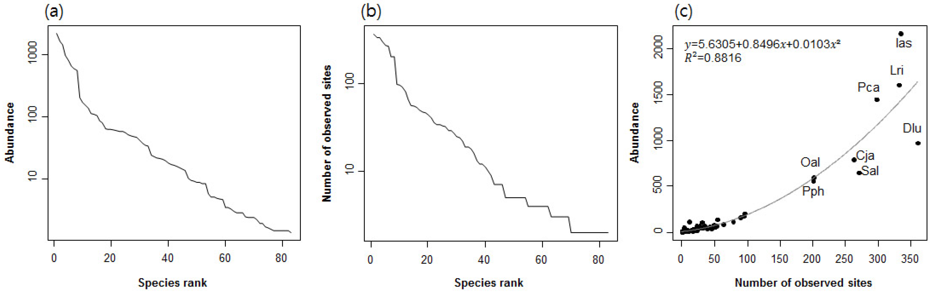
3.1. Distribution Patterns of Species

Our dataset consisted of 965 sampling sites, in which a total of 83 odonatan taxa belonging to 10 families were recorded. Nineteen taxa belonged to the suborder Zygoptera and 64 taxa to the suborder Anisoptera. Abundance and incidence both decreased logarithmically as species rank increased (Figure 2a,b). There were abrupt changes in both the abundance and incidence between species ranks 8 and 9, suggesting that there were eight distinctly dominant species. The abundances of species exponentially increased as their incidence increased ($R^2$ = 0.882) (Figure 2c). Only eight species, namely Davidius lunatus, Ischnura asiatica, Lamelligomphus ringens, Paracercion calamorum, Sieboldius albardae, Calopteryx japonica, Orthetrum albistylum, and Platycnemis phillopoda, were observed in numbers greater than 500 individuals at more than 200 sampling sites, while most species were present in numbers less than 250 individuals and were found at fewer than 100 sampling sites. I. asiatica was the most abundant species (2162 individuals), followed by L. ringens (1603 individuals) and P. calamorum (1446 individuals). D. lunatus was the most widespread species, having the highest incidence (being recorded at 361 sites), followed by I. asiatica (334 sites) and L. ringens (332 sites).

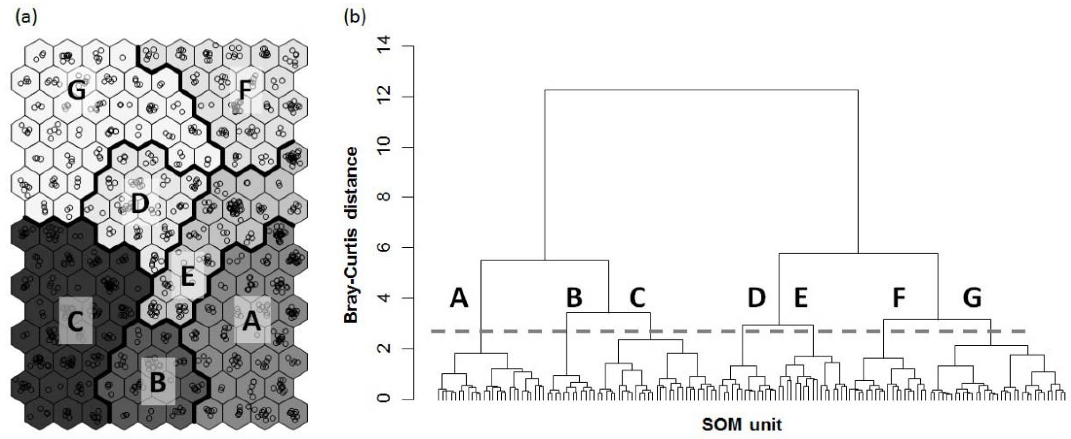
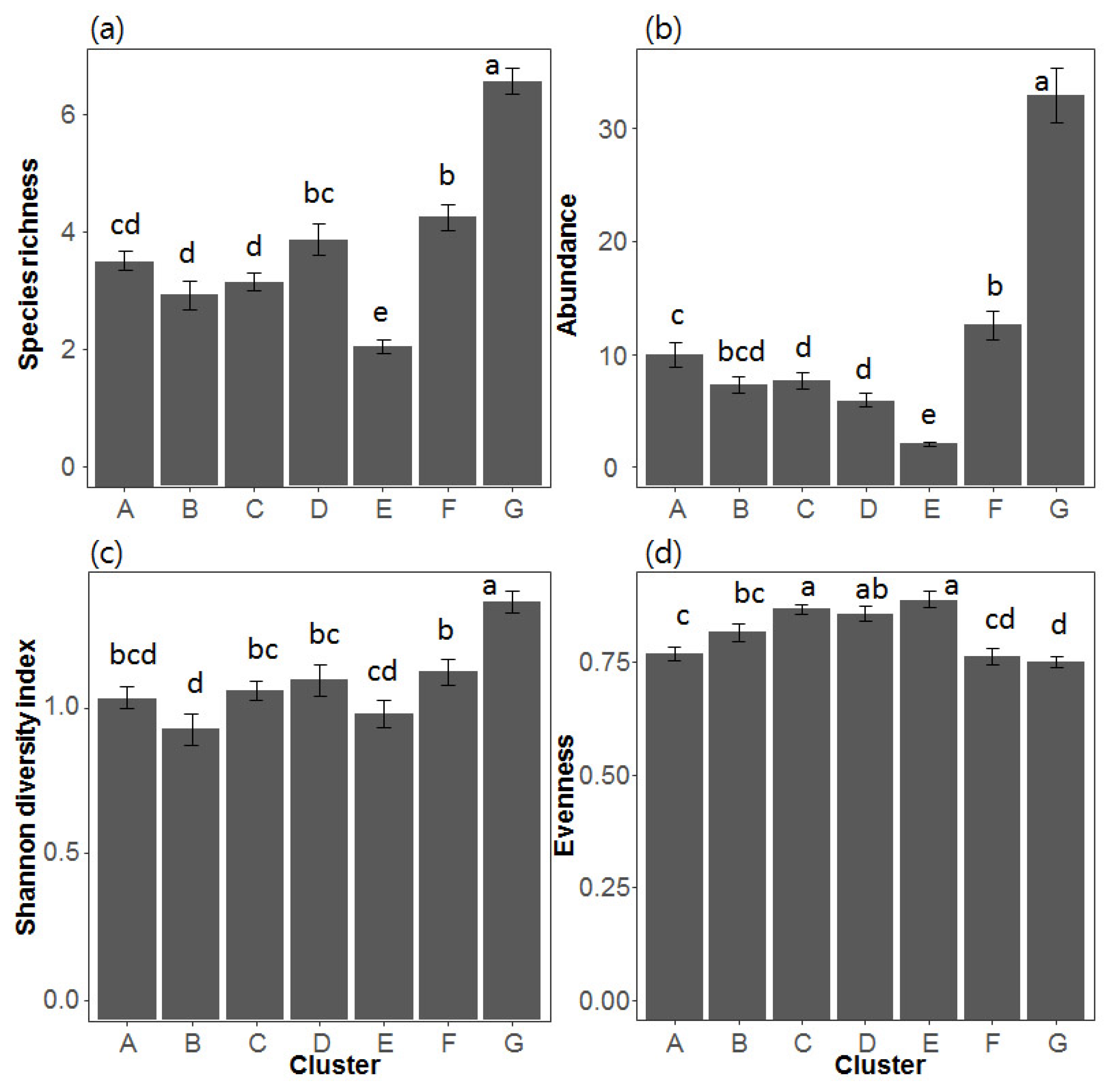
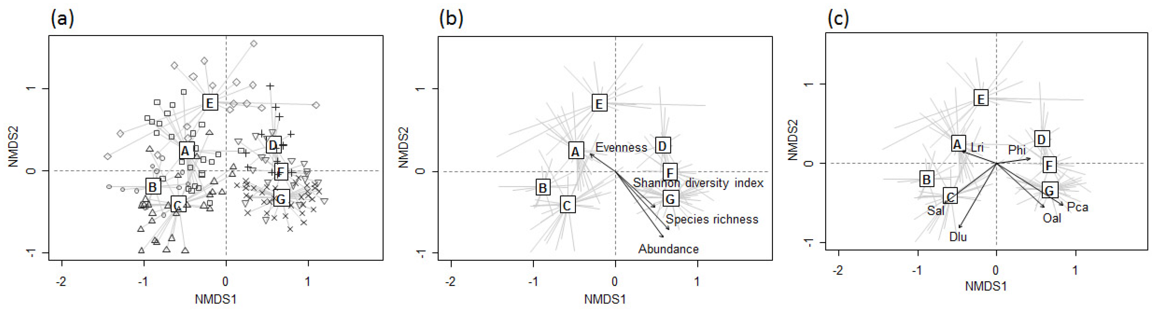
3.2. Patterns in Odonate Assemblages

The SOM projected 965 sampling sites containing 69 taxa onto the SOM output units, according to the observed similarities in odonate assemblages (Figure 3a). SOM output units were split into seven clusters (A–G) based on the dendrogram generated by hierarchical cluster analysis (Figure 3b). These clusters were further divided into two groups (A–C and D–G). Clusters A–C (located on the lower part of the SOM map) were characterized by species of the suborder Anisoptera, whereas clusters D–G (located in the upper part of the SOM map) were characterized by species of the suborder Zygoptera. L. ringens, S. albardae, and D. lunatus were dominant in clusters A, B, and C, respectively. In cluster D, P. calamorum was dominant, and C. atrata, which was the ninth-most dominant species at the nationwide scale, was dominant in cluster E. I. asiatica was dominant in both clusters F and G.

Indicator species were defined in each cluster based on their IndVal (

Table 2. Indicator species of each cluster based on the IndVal.

Suborder	Family	Species	Frequency	Cluster	Stat *	p-Value
Anisoptera	Gomphidae	Lamelligomphus ringens	332	A	0.789	<0.001
Anisoptera	Gomphidae	Ophiogomphus obscura	64	A	0.332	<0.001
Anisoptera	Gomphidae	Sieboldius albardae	271	B	0.791	<0.001
Anisoptera	Corduliidae	Macromia amphigena	54	B	0.246	0.003
Anisoptera	Gomphidae	Davidius lunatus	361	C	0.692	<0.001
Zygoptera	Coenagrionidae	Paracercion hieroglyphicum	33	D	0.259	<0.001
Anisoptera	Corduliidae	Macromia manchuria	43	D	0.219	0.003
Zygoptera	Lestidae	Lestes sponsa	6	D	0.135	0.044
Anisoptera	Libellulidae	Orthetrum albistylum	202	F	0.446	<0.001
Anisoptera	Libellulidae	Pantala flavescens	23	F	0.224	0.003
Anisoptera	Libellulidae	Sympetrum parvulum	6	F	0.198	<0.001
Anisoptera	Libellulidae	Sympetrum kunckeli	11	F	0.139	0.046
Zygoptera	Coenagrionidae	Paracercion calamorum	298	G	0.684	<0.001
Zygoptera	Coenagrionidae	Ischnura asiatica	334	G	0.661	<0.001
Zygoptera	Calopterygidae	Calopteryx japonica	263	G	0.548	<0.001
Zygoptera	Platycnemididae	Platycnemis phillopoda	201	G	0.452	<0.001
Anisoptera	Aeshnidae	Anax parthenope	79	G	0.431	<0.001
Zygoptera	Platycnemididae	Copera annulata	95	G	0.387	<0.001
Anisoptera	Libellulidae	Deielia phaon	49	G	0.344	<0.001
Anisoptera	Libellulidae	Crocothemis servilia	90	G	0.32	<0.001
Anisoptera	Libellulidae	Libellula quadrimaculata	28	G	0.261	<0.001
Zygoptera	Coenagrionidae	Enallagma cyathigerum	33	G	0.241	0.002
Zygoptera	Calopterygidae	Atrocalopteryx atrata	96	G	0.219	0.029
Anisoptera	Aeshnidae	Anax nigrofasciatus	15	G	0.210	0.003
Anisoptera	Gomphidae	Shaogomphus postocularis	32	G	0.200	0.009
Anisoptera	Libellulidae	Orthetrum lineostigma	39	G	0.180	0.024
Anisoptera	Corduliidae	Epitheca marginata	21	G	0.165	0.021

* Stat: statistical value of IndVal in square root.

). The number of indicator species varied between 1 and 15, among the clusters, and cluster E contained no indicator species whatsoever. Clusters A and B contained two indicators species. L. ringens (IndVal statistic = 0.789, p < 0.001) in A and S. albardae (IndVal statistic = 0.791, p < 0.001) in B were indicative species. D. lunatus (IndVal statistic = 0.692, p < 0.001) characterized cluster C, and Paracercion hieroglyphicum (IndVal statistic = 0.259, p < 0.001) characterized cluster D with the highest statistical value among the three total indicator species. Orthetrum albistylum (IndVal statistic = 0.446, p < 0.001) was the most indicative among the four indicator species in cluster F. Eighteen indicator species were present in cluster G, and four species among them were dominant on the nationwide scale. All eight dominant species on the nationwide scale were designated as indicator species.

Community indices were higher in clusters in the upper parts of the SOM map (clusters D–G), and all indices, except evenness, were significantly higher in cluster G, when compared with other clusters (Figure 4). Evenness was significantly lower in cluster G relative to the other clusters. The virtual odonate assemblages split into 150 SOM units were ordinated on the first two axes of the NMDS, reflecting the different clusters produced by the SOM (Figure 5a). SOM units placed in different clusters are indicated by different letters. Community indices and indicator species suitably reflected the differences among clusters (Figure 5b,c).

3.3. Differences in Environmental Variables among Different Assemblage Patterns

NMDS ordination characterized differences in the environmental variables that were divided into six categories. Among the geographical variables, altitude was the most correlated with the NMDS axes ($r^2$ = 0.577, p < 0.01) (Figure 6). Minimum temperature in January was the most contributing variable ($r^2$ = 0.536, p < 0.01) among all meteorological variables, followed by annual average temperature ($r^2$ = 0.485, p < 0.01). In the land use category, the proportion of forest was the most determinant ($r^2$ = 0.631, p < 0.01), followed by the proportion of agricultural land area ($r^2$ = 0.3822, p < 0.01). Considering substrate composition, the proportion of cobble ($r^2$ = 0.565, p < 0.01) had the highest relationship with the NMDS ordination axes, followed by that of silt ($r^2$ = 0.561, p < 0.01). Among the hydrological variables, the proportion of riffle was the most correlated ($r^2$ = 0.425, p < 0.01), and, among the physicochemical variables, BOD displayed the strongest relationship with the NMDS axes ($r^2$ = 0.479, p < 0.01), followed by chlorophyll-a ($r^2$ = 0.369, p < 0.01).

Environmental factors that were deemed important determinants of odonate assemblage patterns by the NMDS analysis were selected for analysis of their magnitudes across SOM clusters (Figure 7). Among geographical variables, altitude and stream order were selected and were highest in clusters B and C and lowest in clusters D, F and G (Dunn test, p < 0.05). Among the meteorological variables, minimum temperature in January and average temperature were selected, and were found to be significantly higher in clusters F and G than in clusters A, B and C (Dunn test, p < 0.05). Among the land use variables, forest (%) was the highest in cluster B but the lowest in cluster F (Dunn test, p < 0.05). When agriculture (%) was high, forest (%) was frequently low, suggesting some kind of inverse relationship between the two. Among substrate composition, cobble (%) was the highest in cluster C and the lowest in clusters D, F and G. Silt (%) was negatively related to cobble (%). Among the hydrological variables, riffle (%) was the highest in cluster C and current velocity was commonly associated with riffle (%) (Dunn test, p < 0.05). Among the physicochemical variables, BOD and chlorophyll-a exhibited similar patterns, being the highest in clusters D–G and the lowest in clusters A–C (Dunn test, p < 0.05). Altitude, forest (%), cobble (%), riffle (%), and current velocity were higher in clusters A–C located in the lower parts of SOM map than in clusters D–G, which were located in the upper parts. Conversely, minimum temperature in January, annual average temperature, agriculture (%), silt (%), BOD, and chlorophyll-a were lower in clusters A–C than in clusters D–G. BOD and silt (%) were significantly lower at higher altitudes, and higher when land area was low.

We selected eight dominant indicator species, which showed high abundances and incidences (observed at more than 200 sampling sites) (Figure 2c and Table 2) to evaluate any differences in their environmental conditions (

Table 3. Differences (mean $\pm$SE) of environmental variables among selected indicator species in each cluster. Different letters present significant differences between species based on Dunn’s multiple comparison test (p < 0.05). We selected eight dominant indicator species which showed occurrence frequency which were observed at more than 200 sampling sites, as shown Figure 2c.

Cluster	Species	Environmental Variables
		Altitude (m)	Temperature (°C) *	Forest (%)	Cobble (%)	Riffle (%)	BOD (mg/L)
A	Lamelligomphus ringens	110.0 (4.3) b	−8.9 (0.1) c	44.2 (1.2) b	21.0 (0.5) b	20.6 (0.8) a	1.5 (0.0) c
B	Sieboldius albardae	147.2 (6.4) a	−9.3 (0.2) c	58.8 (1.5) a	23.4 (0.5) a	24.6 (1.2) a	1.2 (0.0) e
C	Davidius lunatus	150.8 (7.4) b	−9.0 (0.1) c	55.4 (1.4) a	21.7 (0.5) b	25.2 (1.0) a	1.4 (0.0) d
F	Orthetrum albistylum	50.9 (3.2) d	−6.9 (0.2) a	31.0 (1.7) d,e	11.7 (0.7) d	11.6 (1.1) c	2.4 (0.1) a
G	Paracercion calamorum	61.9 (3.9) d	−6.9 (0.1) a	32.7 (1.4) d	12.7 (0.6) d	11.4 (0.9) c	2.2 (0.1) b
G	Ischnura asiatica	54.0 (3.0) d	−6.7 (0.1) a	28.0 (1.3) e	12.0 (0.5) d	12.9 (1.0) c	2.4 (0.1) a
G	Calopteryx japonica	90.9 (4.8) c	−7.7 (0.2) b	38.9 (1.5) c	17.3 (0.6) c	18.3 (1.0) b	1.6 (0.1) c
G	Platycnemis phillopoda	62.2 (4.6) d	−7.2 (0.1) a	33.1 (1.7) d,e	12.2 (0.7) d	11.4 (1.1) c	2.3 (0.1) a,b

* Minimum temperature in January.

). Among the eight dominant species, one indicator species in each of the clusters A, B, C, and F were chosen, and four indicator species in cluster G were selected. Species S. albardae in cluster B was characterized by high-altitudes, whereas species O. albistylum in cluster F, and P. calamorum, Ichnura asiatica, and P. phillopoda in cluster G were more commonly observed in low-altitude areas. L. ringens in cluster A and D. lunatus in cluster C inhabited habitats with similar environmental conditions to S. albardae, but usually at slightly lower altitudes. No dominant indicator species were used in clusters D and E.

4. Discussion

Our dataset contains 83 recorded odonatan species from streams and rivers. Among them, eight species, namely Davidius lunatus, Ischnura asiatica, Lamelligomphus ringens, Paracercion calamorum, Sieboldius albardae, Calopteryx japonica, Orthetrum albistylum, and Platycnemis phillopoda, were dominant with very high incidences (Figure 2). These species were also selected as indicator species. Clusters A–C were dominated by Anisopterans, whereas clusters D–G were characterized by Zygopterans. The differential dominance of these indicator species was mainly due to differences in species habitat preferences as well as differences in their biological and ecological characteristics. For example, Zygopterans typically prefer habitats with a deep and constant water level (e.g., downstream areas) and are weaker fliers over longer distances, whereas Anisopterans primarily inhabit upstream habitats close to forested areas [5].

The distributions of larval odonates is influenced by various scaled environmental factors from microhabitat conditions including water quality and substrate composition to landscape and climate characteristics. For example, NMDS revealed that the altitude, forest ratio (%) in the riparian area, and cobble ratio (%) in substrate composition were the most important environmental factors contributing to differences in odonate assemblage compositions in Korea. Forestation in the riparian area provides important refugia for odonates, allowing them to hide from predators and more effectively hunt prey [38]. The composition of forests and seasonal differences in upstream habitats also affects the structure of benthic macroinvertebrate assemblages including the compositions of odonate assemblages [39,40]. For instance, decreases in canopy cover results in increased sunlight penetration, warmer temperatures, and altered vegetation structure, which can all influence the distribution range, growth rate, and behavior of odonatan species [41]. The presence of vegetation is especially important to some odonatan species such as C. japonica [2,42], although most species are not strictly associated with any particular riparian macrophyte [43]. For example, C. japonica uses macrophytes as both refugia [16] and in their spawning [44]. Calopteryx sp. prefers large substrates when vegetation is sparse, and the influence of substrate size decreases gradually as vegetation density increases [13,45]. Paracercion hieroglyphicum characterized cluster D and is found in lentic waters with rich riparian vegetation [44]. Sampling sites in cluster D were mostly downstream sites with open canopies and high chlorophyll-a concentrations, suggesting that high sunlight penetration unites assemblages in cluster D. Paracercion requires more sunlight than Anisopteran species such as O. albistylum [46,47] as higher temperatures facilitate flight and mating in Zygopteran species. Geographical separation (e.g., habitat fragmentation) is also an important determinant of species distributions [40].

Altitude and the ratio of cobble to silt in substrata were also important in determining odonate assemblage structures in NMDS. Although odonate species are generally known as taxa adapted to warm temperatures and lowland habitats [48], the species D. lunatus and S. albardae are characteristic of the least disturbed areas and are dominant and representative indicator species in mountainous areas (clusters B and C in Figure 7). Similarly, Harabiš and Dolný [49] reported that altitudinal ranges are associated with dragonfly distributions. Sampling sites in cluster F were mostly from agricultural and urban land areas with low canopy coverage and high turbidity. These environmental characteristics were well characterized by the indicator species O. albistylum which is a tactile predator [50] and is tolerant to physicochemical pollution [44]. As they are more competitive than visual predators in turbid environments, they may dominate in these sampling sites. Substrate size is strongly related to habitat condition, influencing organisms’ life cycles and behavior. Many species in Gomphidae are lithophilous and live in association with stony substrata within the lotic habitats. Meanwhile, species such as L. ringens, an indicator species in cluster A, preferred finer substrate sizes as they burrow into the substrate to hide from predators [16]. Our study also showed that cluster G was characterized by silty substrata, as indicated by the identification of the silt-preferring Calopteryx sp. which needs vegetation as an indicator species [9,45].

5. Conclusions

Our research investigated the distribution patterns of odonate species in streams and factors influential in the determination of odonate assemblage compositions on a nationwide scale in South Korea. A total of 83 odonatan taxa belonging to 10 families were recorded in our dataset consisted of 965 sampling sites. Among them, eight species, Davidius lunatus, Ischnura asiatica, Lamelligomphus ringens, Paracercion calamorum, Sieboldius albardae, Calopteryx japonica, Orthetrum albistylum, and Platycnemis phillopoda, displayed distinctly high abundance and incidence. The abundances of species exponentially increased as their incidence increased. Sampling sites were classified into seven different clusters based on differences in odonate assemblage compositions and environmental conditions based on SOM and cluster analysis. Sampling sites were clearly differentiated between being dominated by members of the suborder Anisoptera or the suborder Zygoptera. Among the eight dominant species, S. albardae in cluster B was characterized by high-altitudes, whereas O. albistylum in cluster F, and P. calamorum, Ichnura asiatica, and P. phillopoda in cluster G were more commonly observed in low-altitude areas. L. ringens in cluster A and D. lunatus in cluster C inhabited habitats with similar environmental conditions to S. albardae, but usually at slightly lower altitudes. Indicator species in each cluster had different habitat preferences. Particularly, differences of altitude, forest (%), and cobble (%) in substrata were mainly responsible for variation in assemblage compositions and the determination of indicator species. Finally, our results showed the importance of habitat heterogeneity by demonstrating its effect on odonate assemblage patterns.

References

1. Park, Y.-S.; Céréghino, R.; Compin, A.; Lek, S. Applications of artificial neural networks for patterning and predicting aquatic insect species richness in running waters. Ecol. Model. 2003, 160, 265–280. [Google Scholar] [CrossRef]
2. Goertzen, D.; Suhling, F. Promoting dragonfly diversity in cities: Major determinants and implications for urban pond design. J. Insect Conserv. 2013, 17, 399–409. [Google Scholar] [CrossRef]
3. Corbet, P.S. Dragonflies: Behavior and Ecology of Odonata; Comstock Pub. Associates: Ithaca, NY, USA, 1999; ISBN 978-0-8014-2592-9. [Google Scholar]
4. Kalkman, V.J.; Clausnitzer, V.; Dijkstra, K.-D.B.; Orr, A.G.; Paulson, D.R.; van Tol, J. Global diversity of dragonflies (Odonata) in freshwater. In Freshwater Animal Diversity Assessment; Balian, E.V., Lévêque, C., Segers, H., Martens, K., Eds.; Developments in Hydrobiology, Springer Netherlands: Dordrecht, The Netherlands, 2008; pp. 351–363. ISBN 978-1-4020-8259-7. [Google Scholar]
5. Osborn, R.; Samways, M.J. Determinants of adult dragonfly assemblage patterns at new ponds in South Africa. Odonatologica 1996, 25, 49–58. [Google Scholar]
6. Kutcher, T.E.; Bried, J.T. Adult Odonata conservatism as an indicator of freshwater wetland condition. Ecol. Indic. 2014, 38, 31–39. [Google Scholar] [CrossRef]
7. Hassall, C. Odonata as candidate macroecological barometers for global climate change. Freshw. Sci. 2015, 34, 1040–1049. [Google Scholar] [CrossRef]
8. Jonsson, M.; Johansson, F.; Karlsson, C.; Brodin, T. Intermediate predator impact on consumers weakens with increasing predator diversity in the presence of a top-predator. Acta Oecol. Int. J. Ecol. 2007, 31, 79–85. [Google Scholar] [CrossRef]
9. Brooks, S. Field Guide to the Dragonflies and Damselfies of Great Britain and Ireland; Bloomsbury Publishing Inc.: New York, NY, USA, 2018; ISBN 978-1-4729-6453-3. [Google Scholar]
10. Foote, A.L.; Hornung, C.L.R. Odonates as biological indicators of grazing effects on Canadian prairie wetlands. Ecol. Entomol. 2005, 30, 273–283. [Google Scholar] [CrossRef]
11. Villalobos-Jimenez, G.; Dunn, A.; Hassall, C. Dragonflies and damselflies (Odonata) in urban ecosystems: A review. Eur. J. Entomol. 2016, 113, 217–232. [Google Scholar] [CrossRef] [Green Version]
12. Renner, S.; Périco, E.; Dalzochio, M.S.; Sahlén, G. Water body type and land cover shape the dragonfly communities (Odonata) in the Pampa biome, Rio Grande do Sul, Brazil. J. Insect Conserv. 2018, 22, 113–125. [Google Scholar] [CrossRef]
13. Hofmann, T.A.; Mason, C.F. Habitat characteristics and the distribution of Odonata in a lowland river catchment in eastern England. Hydrobiologia 2005, 539, 137–147. [Google Scholar] [CrossRef]
14. Sahlén, G.; Ekestubbe, K. Identification of dragonflies (Odonata) as indicators of general species richness in boreal forest lakes. Biodivers. Conserv. 2001, 10, 673–690. [Google Scholar] [CrossRef]
15. Ruggiero, A.; Céréghino, R.; Figuerola, J.; Marty, P.; Angélibert, S. Farm ponds make a contribution to the biodiversity of aquatic insects in a French agricultural landscape. C. R. Biol. 2008, 331, 298–308. [Google Scholar] [CrossRef] [PubMed]
16. Jung, K. Odonata Larvae of Korea; Nature & Ecology: Seoul, Korea, 2012; ISBN 978-89-962995-6-1. (In Korean) [Google Scholar]
17. Park, Y.-S.; Song, M.-Y.; Park, Y.-C.; Oh, K.-H.; Cho, E.; Chon, T.-S. Community patterns of benthic macroinvertebrates collected on the national scale in Korea. Ecol. Model. 2007, 203, 26–33. [Google Scholar] [CrossRef]
18. Li, F.; Chung, N.; Bae, M.-J.; Kwon, Y.-S.; Park, Y.-S. Relationships between stream macroinvertebrates and environmental variables at multiple spatial scales. Freshw. Biol. 2012, 57, 2107–2124. [Google Scholar] [CrossRef]
19. Ministry of Environment (MOE), National Institute of Environmental Research (NIER). Survey and Evaluation Method for River and Stream Ecosystem Health Assessment; MOE, NIER: Incheon, Korea, 2015. (In Korean) [Google Scholar]
20. Bae, M.-J.; Kwon, Y.; Hwang, S.-J.; Chon, T.-S.; Yang, H.-J.; Kwak, I.-S.; Park, J.-H.; Ham, S.-A.; Park, Y.-S. Relationships between three major stream assemblages and their environmental factors in multiple spatial scales. Ann. Limnol. Int. J. Limnol. 2011, 47, S91–S105. [Google Scholar] [CrossRef] [Green Version]
21. Ministry of Land, Infrastructure and Transport (MOLIT), Han River Flood Control Office (HRFCO). List of Rivers of South Korea; MOLIT: Sejong, Korea, 2013. (In Korean) [Google Scholar]
22. Jeju Development Institute. The Hydrologic and Water Quality Characteristics Analysis for the Streamwater Application in Jeju Island; Jeju Development Institute: Jeju, Korea, 2009. (In Korean) [Google Scholar]
23. Environmental Systems Research Incorporated (ESRI). ArcGIS 10.1; Environmental Systems Research Incorporated: Redlands, CA, USA, 2013. [Google Scholar]
24. American Public Health Association. Standard Methods for the Examination of Water and Wastewater; American Public Health Association/American Water Works Association/Water Environment Federation: Washington, DC, USA, 2005. [Google Scholar]
25. Cummins, K.W.; Lauff, G.H. The influence of substrate particle size on the microdistribution of stream macrobenthos. Hydrobiologia 1969, 34, 145–181. [Google Scholar] [CrossRef]
26. Kohonen, T. Self-organized formation of topologically correct feature maps. Biol. Cybern. 1982, 43, 59–69. [Google Scholar] [CrossRef]
27. Park, Y.-S.; Kwon, Y.-S.; Hwang, S.-J.; Park, S. Characterizing effects of landscape and morphometric factors on water quality of reservoirs using a self-organizing map. Environ. Model. Softw. 2014, 55, 214–221. [Google Scholar] [CrossRef]
28. Céréghino, R.; Park, Y.-S. Review of the Self-Organizing Map (SOM) approach in water resources: Commentary. Environ. Model. Softw. 2009, 24, 945–947. [Google Scholar] [CrossRef]
29. Vesanto, J. Neural Network Tool for Data Mining: SOM Toolbox. In Proceedings of the TOOLMET 2000—3rd International Symbosium on Tool Environments and Development Methods for Intelligent Systems, Oulu, Finland, 13–14 April 2000; pp. 152–169. [Google Scholar]
30. Park, Y.-S.; Tison, J.; Lek, S.; Giraudel, J.-L.; Coste, M.; Delmas, F. Application of a self-organizing map to select representative species in multivariate analysis: A case study determining diatom distribution patterns across France. Ecol. Inform. 2006, 1, 247–257. [Google Scholar] [CrossRef]
31. Dufrene, M.; Legendre, P. Species Assemblages and Indicator Species: The Need for a Flexible Asymmetrical Approach. Ecol. Monogr. 1997, 67, 345–366. [Google Scholar] [CrossRef]
32. De Cáceres, M.D.; Jansen, F. Indicspecies: Relationship between Species and Groups of Sites. R Package Version 1.7.6. Available online: https://cran.r-project.org/web/packages/indicspecies/ (accessed on 24 October 2018).
33. Shepard, R.N. The analysis of proximities: Multidimensional scaling with an unknown distance function. II. Psychometrika 1962, 27, 219–246. [Google Scholar] [CrossRef]
34. R Development Core Team. R: A Language and Environment for Statistical Computing; R Foundation for Statistical Computing: Vienna, Austria, 2011; Available online: http://www.R-project.org (accessed on 6 September 2017).
35. Pohlert, T. PMCMR: Calculate Pairwise Multiple Comparisons of Mean Rank Sums. R Package Version 4.3. Available online: https://CRAN.R-project.org/package=PMCMR (accessed on 24 October 2018).
36. Wehrens, R.; Kruisselbrink, J. kohonen: Supervised and Unsupervised Self-Organising Maps. R Package Version 3.0.6. Available online: https://CRAN.R-project.org/package=kohonen (accessed on 24 October 2018).
37. Oksanen, J.; Blanchet, F.G.; Friendly, M.; Kindt, R.; Legendre, P.; McGlinn, D.; Minchin, P.R.; O’Hara, R.B.; Simpson, G.L.; Solymos, P.; et al. Vegan: Community Ecology Package. R Package Version 2.5-2. Available online: https://CRAN.R-project.org/package=vegan (accessed on 24 October 2018).
38. Clausnitzer, V.; Kalkman, V.J.; Ram, M.; Collen, B.; Baillie, J.E.M.; Bedjanič, M.; Darwall, W.R.T.; Dijkstra, K.-D.B.; Dow, R.; Hawking, J.; et al. Odonata enter the biodiversity crisis debate: The first global assessment of an insect group. Biol. Conserv. 2009, 142, 1864–1869. [Google Scholar] [CrossRef]
39. Bae, M.-J.; Chun, J.; Chon, T.-S.; Park, Y.-S.; Bae, M.-J.; Chun, J.H.; Chon, T.-S.; Park, Y.-S. Spatio-Temporal Variability in Benthic Macroinvertebrate Communities in Headwater Streams in South Korea. Water 2016, 8, 99. [Google Scholar] [CrossRef]
40. Lee, D.-Y.; Bae, M.-J.; Kwon, Y.-S.; Park, C.-W.; Yang, H.M.; Shin, Y.; Kwon, T.-S.; Park, Y.-S. Characteristics of Spatiotemporal Patterns in Benthic Macroinvertebrate Communities in Two Adjacent Headwater Streams. Korean J. Ecol. Environ. 2018, 51, 192–203. [Google Scholar] [CrossRef]
41. Suh, A.N.; Samways, M.J. Significance of temporal changes when designing a reservoir for conservation of dragonfly diversity. Biodivers. Conserv. 2005, 14, 165–178. [Google Scholar] [CrossRef]
42. Van de Meutter, F.; Meester, L.D.; Stoks, R. Water turbidity affects predator–prey interactions in a fish–damselfly system. Oecologia 2005, 144, 327–336. [Google Scholar] [CrossRef] [PubMed]
43. Lombardo, P. Predation by Enallagma nymphs (Odonata, Zygoptera) under different conditions of spatial heterogeneity. Hydrobiologia 1997, 356, 1–9. [Google Scholar] [CrossRef]
44. Jung, K. Odonata of Korea; Ilgongyuksa: Seoul, Korea, 2007; ISBN 978-89-958060-3-6. (In Korean) [Google Scholar]
45. Ward, L.; Mill, P.J. Substrate selection in larval Calopteryx splendens (Harris) (Zygoptera: Calopterygidae). Odonatologica 2008, 37, 69–77. [Google Scholar]
46. Samejima, Y.; Tsubaki, Y. Body temperature and body size affect flight performance in a damselfly. Behav. Ecol. Sociobiol. 2010, 64, 685–692. [Google Scholar] [CrossRef]
47. Tsubaki, Y.; Samejima, Y.; Siva-Jothy, M.T. Damselfly females prefer hot males: Higher courtship success in males in sunspots. Behav. Ecol. Sociobiol. 2010, 64, 1547–1554. [Google Scholar] [CrossRef]
48. Kalcounis-Rueppell, M.C.; Payne, V.H.; Huff, S.R.; Boyko, A.L. Effects of wastewater treatment plant effluent on bat foraging ecology in an urban stream system. Biol. Conserv. 2007, 138, 120–130. [Google Scholar] [CrossRef]
49. Harabis, F.; Dolny, A. Ecological factors determining the density-distribution of Central European dragonflies (Odonata). Eur. J. Entomol. 2010, 107, 571–577. [Google Scholar] [CrossRef] [Green Version]
50. Sahlén, G.; Haase, S.; Suhling, F. Morphology of dragonfly larvae along a habitat gradient: Interactions with feeding behaviour and growth (Odonata: Libellulidae). Int. J. Odonatol. 2008, 11, 225–240. [Google Scholar] [CrossRef]
Figure 1. (a) Location of sampling sites; and (b) altitudinal map of South Korea.
Insects 09 00152 g001
Figure 2. (a) Species rank-abundance curve; (b) species rank-incidence curve; and (c) relationship between species abundance and incidence. Three letters in Figure 2c are abbreviations for the eight dominant species: Ias, Ischnura asiatica; Lri, Lamelligomphus ringens; Dlu, Davidius lunatus; Pca, Paracercion calamorum; Sal, Sieboldius albardae; Cja, Calopteryx japonica; Oal, Orthetrum albistylum; Pph, Platycnemis phillopoda.
Insects 09 00152 g002
Figure 3. (a) Classification of sampling sites using a Self-organizing map (SOM); and (b) classification of SOM units based on the dendrogram of hierarchical cluster analysis with Ward linkage methods using Bray–Curtis distances. Weight vectors of SOM units were used in the hierarchical cluster analysis.
Insects 09 00152 g003
Figure 4. Differences in community indices: (a) species richness (number of species); (b) abundance (number of individuals); (c) Shannon diversity index; and (d) evenness. Different letters represent significant differences between clusters based on Dunn’s multiple comparisons test (p < 0.05). Error bars indicate standard errors.
Insects 09 00152 g004
Figure 5. (a) The NMDS ordination of odonate assemblages based on the weight vectors of SOM units (stress value: 0.203); (b) biplots with community indices; and (c) the most significant indicator species in each cluster. Abbreviations for indicator species are given in Table 2.
Insects 09 00152 g005
Figure 6. Biplots of environmental variables in six different categories of NMDS ordination: (a) Geography; (b) meteorology; (c) land use; (d) substrate composition; (e) hydrology; and (f) physicochemical water quality. Abbreviations for the variables are given in Table 1.
Insects 09 00152 g006
Figure 7. Differences in environmental variables in the seven different clusters. Different letters represent significant differences among clusters based on Dunn’s multiple comparisons tests (p < 0.05). Error bar represents the standard error in each cluster.
Insects 09 00152 g007