Collecting Labels for Rare Anomalies via Direct Human Feedback—An Industrial Application Study


1
Department of Electrical Engineering and Computer Science, University of Siegen, 57068 Siegen, Germany
2
Corporate Research, Robert Bosch GmbH, 71272 Renningen, Germany
*
Author to whom correspondence should be addressed.
Informatics 2019, 6(3), 38; https://doi.org/10.3390/informatics6030038
Submission received: 29 July 2019
/
Revised: 23 August 2019
/
Accepted: 29 August 2019
/
Published: 2 September 2019
Abstract
:Many systems rely on the expertise from human operators, who have acquired their knowledge through practical experience over the course of many years. For the detection of anomalies in industrial settings, sensor units have been introduced to predict and classify such anomalous events, but these critically rely on annotated data for training. Lengthy data collection campaigns are needed, which tend to be combined with domain expert annotations of the data afterwards, resulting in costly and slow process. This work presents an alternative by studying live annotation of rare anomalous events in sensor streams in a real-world manufacturing setting by experienced human operators that can also observe the machinery itself. A prototype for visualization and in situ annotation of sensor signals is developed with embedded unsupervised anomaly detection algorithms to propose signals for annotation and which allows the operators to give feedback on the detection and classify anomalous events. This prototype allowed assembling a corpus of several weeks of sensor data measured in a real manufacturing surrounding and was annotated by domain experts as an evaluation basis for this study. The evaluation of live annotations reveals high user motivation after getting accustomed to the labeling prototype. After this initial period, clear anomalies with characteristic signal patterns are detected reliably in visualized envelope signals. More subtle signal deviations were less likely to be confirmed an anomaly due to either an insufficient visibility in envelope signals or the absence of characteristic signal patterns.
1. Introduction
Collecting labels for rare anomalous events is notoriously difficult. Often, frequent spurious signal outliers dominate seemingly detected anomalies and shadow the few, real anomalies. This is even more difficult when anomalies are characterized by more subtle signal deviations than these spurious signal outliers. Depending on the chosen anomaly detection algorithm, this dominance of spurious outliers typically results in either a high false positive rate (FPR) or false negative rate (FNR). This is even more the case for purely unsupervised models.
While a large amount of studies on collecting rare event labels in medical or social applications exists, this study is concerned with industrial manufacturing surroundings. In the chosen machine tool monitoring application, spurious outliers are given by frequent process adaptations while real anomalies are typically rare. The reason for the latter is that machines in a real-world production surrounding are typically used for processing the same type of workpiece over a long period of time, spanning several months to years. Thus, robust process parameter settings are known due to the well-understood machine behavior for this exact workpiece type, which in turn results in anomalies appearing only rarely.
In order to train anomaly detection models for a subset of specific known anomalies (e.g., imbalance, belt tension, and wear of ball screw drives or spindles), we can intentionally choose insensible process parameters to provoke these types of anomalies. Then, dedicated measurement campaigns for these anomaly types allow for studying how these types of anomalies manifest regarding change of signal behavior. This approach comes with short measurement campaigns (as the precious anomalous labels can be provoked intentionally) and, thus, only a small amount of additional costs due to loss of production time. Furthermore, we obtain high-quality ground truth labels for these anomalies as we control the anomaly-causing machine parameters. However, several drawbacks arise:
- Provoking anomalies is still expensive, as retooling the machine for these provocations is time consuming. Furthermore, precious production time is lost as the anomalously processed workpieces cannot be used after the experiment. Thus, annotating data sets with anomaly labels via dedicated measurement campaigns always comes with a trade-off: The higher the amount of labeled data the better the performance of (semi-)supervised anomaly classifiers but also the higher the loss in production time and thus increase in costs. The availability of annotated datasets that also tend to be limited in size and the inherent cost/accuracy trade-off are well-known problems in industrial manufacturing applications and have led to domain-specific approaches optimizing the predictive quality with the given data sets of limited size [1].
- Many anomalies cannot be provoked intentionally, either due to unknown cause–effect relations of these anomalies or due to severe risks of long-term machine part damages.
- If anomalies can be provoked intentionally, the anomalies do not emerge in a natural way. As it is often nontrivial to distinguish between cause and effect in the signal behavior, it is unclear whether the studied abnormal behavior will generalize to real-world anomalies.
- Finally, only anomaly types known in advance can be provoked.
Thus, collecting data and corresponding annotations “in the wild” has the potential to yield more realistic labels. Typically, these measurement campaigns are combined with retrospective annotation of signals by domain experts. This retrospective annotation by domain expert results in high costs for rare anomaly scenarios, especially when the data is not pre-filtered regarding its preciousness (as a high fraction of measured data will not be illustrating anomalous machine behavior). Furthermore, the context knowledge about machine behavior during data collection is lost.
We propose a third alternative approach by prompting anomalous events to the machine operators for label feedback directly during everyday processing of workpieces. Prompting only suspicious signals for annotation reduces the labeling effort while live annotation minimizes the additional time effort induced by signal annotation. Thus, live annotation allows collecting anomaly labels in the wild for low costs, as we do not have to rely on separate measurement campaigns but can collect data during normal operation of the machine tools. Furthermore, the possibility to visually inspect the machine gives the machine operators valuable, additional information during live annotation of the collected data. Limitations to this approach might be given by the necessity of giving timely feedback to proposed anomalies (i.e., reduced label quality by time pressure).
For our experiments, we equipped a grinding machine in a real-world production surrounded with multiple microelectromechanical systems (MEMS) vibration sensors for long-term measurements. Additionally, we developed and integrated both hardware and software of a labeling prototype, including the design of a suitable graphical user interface (GUI), for in situ annotation of sensor signals. We developed this new prototype instead of relying on smartphone- or tablet-based human–machine interfaces in order to fulfill requirements regarding the harsh industrial environment. Additionally, smartphones do not allow for a sufficiently large and detailed visualization of the sensor signals, which is crucial for providing machine operators with the necessary information for reliable live annotation (cf. Section 6.2.2, Section 6.2.4, and Section 6.2.5). The physical prototype device was attached to the outside of the machine and connected to these sensors (cf. Figure 1).
Potential abnormal events are detected by a generic unsupervised anomaly detection model. The unsupervised anomaly detection model can then raise an alarm (both acoustically and by activation of a flash light) to trigger feedback of the human machine operator to the proposed anomaly. The visualization of sensor signals at the prototype comes with a GUI which guides the labeling process and additionally allows for user-initiated labeling of anomalies and process adaptations. Thus, we aim to achieve a large-scale data set of several weeks of sensor signals and related in-the-wild labels annotated by domain experts directly in the setting they were recorded. Training (semi-)supervised extensions of the unsupervised anomaly detection model by incorporating these live annotations will be part of future work.
The major challenge of our approach from an algorithmic point of view lies in the choice of an appropriate generic anomaly detection model. Guided by theoretically formulated constraints given by the embedded nature of our system, the characteristics of our data, and the behavior of machine operators, we perform tests on a labeled subset of our data for an initial choice of anomaly detection model. The best-performing algorithm is then chosen for deployment on our demonstrator system.
From a human–machine interface point of view, estimating reliability both of anomaly propositions of the chosen anomaly detection model and of human label feedback is challenging due to the fact that, for most of our data, no ground truth labels exist. Furthermore, we cannot rely on comparison of labels from multiple annotators as typical crowd labeling methods do because label feedback is collected from a single annotator (i.e., the current machine operator). We introduce several assumptions both on label reliability and annotator motivation and validate them relying on the amount and distribution of label mismatch between anomaly propositions and online label feedback, labeling behavior of different annotators (inter-annotator agreement) during a second retrospective signal annotation phase, and temporal evolution of labeling behavior of annotators. Furthermore, we investigate the influence of certainty of the anomaly detection algorithm of its anomaly propositions (measured in height of anomaly scores), the familiarity of machine operators with the labeling user interface, and other measures regarding user motivation on the reliability of online label feedback.
In summary, the main questions that we aim to address in this study are as follows:
- Can we collect high-quality but low-cost labels for machine tool anomalies from machine operators’ online label feedback to anomalies proposed by a generic unsupervised anomaly detection algorithm?
- Can we develop a sensible and understandable human–machine interface for the online labeling prototype by taking the end users’ (i.e., machine operators’) opinion into account during the design process?
- Can simple anomaly detection models respecting hardware constraints of our embedded labeling prototype yield sensible anomaly propositions?
- How does the reliability of label feedback depend on the type of anomaly, the kind of signal visualization, and the clarity of proposed anomalies (measured in height of anomaly scores)?
- How can we measure reliability of the annotators’ label feedback sensibly without access to ground truth labels for most of the data and with label feedback from only one annotator at a time (i.e., the current operator of the machine tool)?
The main contributions of this study are as follows:
- We conduct a study exploring how to incorporate domain expert knowledge for online annotation of abnormal rare events in industrial scenarios. To the best of our knowledge, no comparable study exists.
- Other than in the frequent studies on labeling in medical and social applications, we collect labels not via a smartphone-based human–machine interface but via a self-developed visualization and labeling prototype tailor-made for harsh industrial environments.
- We share insights from the process of designing the visualization and labeling interface gathered by exchange with industrial end users (i.e., machine operators).
- We propose measures to judge the quality of anomaly propositions and online label feedback in a scenario where neither ground truth labels are accessible nor comparison of labels of multiple annotators is an option. We evaluate these assumptions on a large corpus (123,942 signals) of real-world industrial data and labels which we collected throughout several weeks.
- Furthermore, we describe which types of anomalies can be labeled reliably with the proposed visualization and labeling prototype and identify influential factors on annotation reliability.
In the remainder of the paper, we first discuss related work on anomaly detection models (Section 2.1) and methods for the evaluation of human annotations (Section 2.2). Then, we introduce several assumptions for the evaluation of quality of the human label feedback provided by the proposed live and in situ annotation approach (Section 3). These assumptions address the challenges of rating label feedback quality without being provided ground truth labels or more than one online annotation per signal. Afterwards, we describe details about the setup for data measurement (Section 4) as well as the design process and functionality of the proposed labeling prototype (Section 5). Then, we state results for the experiments conducted in order to select an appropriate anomaly proposing model (Section 6.1) and in order to rate the quality of labels collected via the proposed live annotation approach (Section 6.2). The latter evaluation of live annotations is guided by the assumptions formulated in Section 3. In Section 7, finally, we summarize the results and critically discuss the strengths and weaknesses of our approach as well as the feasibility to generalize the approach to other application domains.
2. Related Work
2.1. Anomaly Detection
In Reference [2], Chandola et al. distinguished different types of anomalies regarding their relation to the rest of the data. In this study, the focus will be on collective anomalies. This type of anomaly has been characterized by a collection of signal samples being interpreted as anomalous behavior and opposed to point anomalies, which manifest in single outlying signal samples. Furthermore, anomalies considered in this study manifest as contextual anomalies, where the context of signal samples (e.g., relative position in the signal) is relevant for an outlying segment of data being labeled anomalous.
For this intersection of collective and contextual anomalies, a large corpus of potential anomaly detection models can be considered. These models can be distinguished based on the representation of the data used as input for the model:
- One-dimensional representation: Anomaly detection models rely on the data being given as one-dimensional vectors. These vectors can be given as either raw signals or a transformation of the data to another, one-dimensional representation. Popular transformations are envelope signals [3], wavelet-based representations [4], or other spectral transformations based on singular value decompositions [5].
- Multidimensional representations: These representations emerge when the sensor data are projected to a dual space by extraction of features. When aiming for a generic anomaly detection model, the major challenge is given by the choice of a generic but expressive set of features [6]. Among popular choices are statistical measures and wavelet-based features [7] or filter bank features (e.g., Mel-frequency cepstral coefficient (MFCC) features) [8]. The latter yield similar information to anomaly detection approaches based on time-frequency distributions (TFDs).
- TFD representations: Recently, different powerful deep learning approaches capable of learning the latent representations of the underlying, data-generating process from two-dimensional data have been introduced (with a focus on two-dimensional representations, typically images). Among these, deep generative models like variational autoencoders (VAEs) [9], generative adversial networks (GANs) [10], auto-regressive generative models like PixelRNN/CNN [11], and non-autoregressive flow-based models [12,13,14] supersede earlier autoencoder (AE) approaches [15,16,17] which come with a compressed latent representation of the data but without the possibility of generating samples from the latent representation. It is this ability to sample from the generative process of the data which seems to allow deep generative models to capture details of the data flexibly without any access to labels.
In this study, we will focus on one-dimensional representations due to the problems involved with finding a generic feature set for multidimensional feature space approaches.
2.1.1. Methods Based on One-Dimensional Representations
Approaches of direct clustering and classification of one-dimensional time series representations rely on the computation of pairwise time series distance measures. The most common measures are Euclidean distance (ED) and dynamic time warping (DTW) distance [18] as well as its extensions (soft-DTW (SDTW) [19], DTW barycenter averaging (DBA) [20], etc.). While Euclidean distances are calculated directly based on the samples at corresponding signal locations, DTW-related measures come with an additional, preceding step for optimal alignment of signals via nonlinear warping of the time series. This flexibility allows comparison of signals with different lengths or non-uniformly affine transformed signals.
For classification, k-nearest neighbors (kNN) and especially 1NN have evolved as a common baseline [19]. Multiple evaluations have shown that 1NN is hard to beat in time series classification, especially when combined with the DTW measure [21,22]. For large training data sets, it has been shown that the predictive quality with Euclidean distance assimilates to that of elastic measures such as DTW [23]. Unfortunately, kNN suffers from high memory costs and long prediction times as all training examples have to be stored (both for training set size N and signal length T in a naive implementation). To make a prediction on a new time series, the DTW measure has to be computed for all these training examples, resulting in high computational demands and long prediction times. In Reference [24], nearest centroid (NC) combined with DBA has been shown to be competitive with kNN at a much smaller computational cost (i.e., prediction time) and reduced memory space demand across multiple data sets. This has been confirmed in Reference [19] for barycenter averaging with the Soft-DTW measure. The NC methods rely on each anomaly class being sufficiently representable by a single centroid.
Time series clustering methods group training time series into a number of (typically prespecified) clusters. A popular choice in time series analysis is k-means, being the only clustering algorithm scaling linearly with data set size [6]. Here, DTW-based elastic measures might again be used to find the barycenter best representing the centroids of k-means clusters [19]. A computationally efficient alternative is k-medoids, which selects centroids from the set of training data examples, i.e., spares the step of learning centroids from training data samples [25]. Among more advanced clustering approaches, hierarchical clustering approaches like DBSCAN [26] and its variants OPTICS [27] or HDBSCAN [28] are popular choices. They come without (parametric) constraints on cluster forms but find clusters in dense regions of data points. Complementary, subspace clustering techniques like SSC [29] or FSC [30] have superseded traditional clustering techniques by finding a descriptive subspace of the time series data parallel to clustering and are thus more immune to the curse of dimensionality inherent to all time series methods. For a more extensive overview of time series clustering approaches, we refer to the surveys in References [31,32].
Finally, multiple deep learning techniques have started conquering the field on time series methods. Typically approaches based on recurrent neural networks (RNNs) have dominated [33,34], while other approaches based on VAEs [35] or convolutional neural networks (CNNs) [34,36] have only most recently started to appear.
2.1.2. Multidimensional Representation-Based Methods
Feature space methods yield a powerful way to reduce the information given by raw samples in sensor signals. As mentioned above, these approaches come with the challenge of identifying a sensible set of features when we aim for a generic anomaly detection: For a generic anomaly detection, it is typically infeasible to specify the most relevant features a priori. Thus, a potentially large set of features has to be computed. As discussed in Reference [37], high-dimensional feature spaces result in increasing distances between all data points, which makes common approaches of finding anomalies by large distances to normal data points or in regions with a small density of data points increasingly less appropriate. This is known as the curse of dimensionality and has been described first in Reference [38] for applications of high dimensional outlier detection. Thus, feature space approaches in anomaly detection have to come with an implicit or explicit feature selection (e.g., decision tree-based approaches) or dimensionality reduction (e.g., subspace methods) or have to be robust to irrelevant features and the high dimensionality of the feature space (e.g., robust covariance estimators [39]). The challenge of defining the most relevant features a priori for feature space-based methods might alternatively be circumvented by relying on feature learning techniques. Apart from sparse dictionary techniques like nonnegative matrix factorization (NMF), neural network-based methods have dominated the field of feature learning. Despite their dominance in image classification, their application in (time series) anomaly detection fields is rather seldom.
Purely unsupervised, multidimensional anomaly detection approaches model anomalies as outlying points from dense regions of data points [40]. Dense normal regions have been identified either by model-based approaches like one-class classifiers [41,42,43] and probabilistic models [39] or proximity-based approaches. The latter group of algorithms can be further distinguished into distance-based methods (often kNN-based approaches like ODIN [44]) and density-based approaches like LOF [45] and its extensions [46,47,48]. Other popular proximity-based approaches are INFLO [49], LoOP [50], LDOF [51], LDF [52], and KDEOS [53]. More advanced, hierarchical density-based approaches have been introduced by DBSCAN [26] and its extensions like OPTICS [27] or HDBSCAN [28].
Many of the former methods have relied on data being given as complete batch, i.e., data have been considered in an offline classification scenario. Recently, the streaming data scenario (i.e., online classification) has received more attention triggered by the position papers of Aggarwal [54] and Zimek [55]. Dominant techniques have relied on ensemble methods based on the early success of isolation forests [56] and the theoretical analysis of anomaly ensembles in Reference [57]. Recent work on outlier ensembles in streaming data scenarios has been listed in Reference [58] and given by the subsampling techniques in Reference [59], ensembles of randomized space trees [60] or half-space trees [61], selective [62] and sequential [63] anomaly ensembles, histogram-based ensembles like LODA [64], and subspace hashing ensembles like RS-Hash [65] or xStream [58].
2.1.3. Two-Dimensional Representation-Based Methods
In general, two-dimensional representations like TFDs open up perspectives for making use of the numerous methods applied in image processing, among which deep learning approaches have dominated in recent years (cf. Section 2.1). In a follow-up study, we will focus on finding more elaborate and (semi-)supervised anomaly detection methods, including deep learning approaches from the image processing domain. In this study, we will focus on finding and describing ways to collect live annotations via simple anomaly detection models. This will allow us to provide large labeled data sets necessary for these methods considered in the follow-up study.
2.2. Label Evaluation
Classical measures for comparison of two sets of labels are given by precision, recall, and F1 scores. Additionally, the most prominent measures for outlier detection are given by the area under curve (AUC) score for the receiver operating characteristic (ROC) curve and the precision@k measure [66].
All of these measures rely on being given ground truth labels for estimating predictive quality. Despite small subsets of the sensor data labeled by domain experts, we do not have access to such ground truth labels. Additionally, both online annotation of data directly during recording at the machine via the labeling prototype and retrospective annotation to a later point of time (i.e., by being shown only the signals but not having the direct context of when these signals were recorded) can introduce uncertainty into the process of human labeling. Thus, it is a priori not trivial to decide which labels should be considered more reliable: labels proposed by the anomaly detection algorithm, online label feedback by the human annotator, or label feedback during a second retrospective labeling period.
2.2.1. Label Comparison without Knowing a Ground Truth
A vast amount of literature on estimating or improving reliability of human annotations exists. Among the most typical application fields are medical applications like smoking detection [67], sleep detection [68], or affect recognition [69] and the large field of activity recognition [70,71]. While earlier work has focused on collecting labels from diaries filled out by study participants, smartphone apps have taken over the field of human annotation [72,73,74,75]. The main advantage of collecting labels via smart phones is timely labeling triggered by events (e.g., from sensor data) paired with visualization of context data in order to give the user a sensible amount of information during annotation. We built on these strengths by a similar approach relying on our visualization and labeling prototype.
Much of the work on collecting human annotations has focused on active learning scenarios, which prompt the user for annotation only for the data being considered most valuable [37]. High value can be defined, among other strategies, by high uncertainty of the predictive model regarding classification of the given data (which is referred to as uncertainty sampling [76]) or by the scarcity of assumed labels (i.e., rare labels are more valuable). The latter strategy is related to our scenario of detecting rare, abnormal events, where the idea is to get annotator’s feedback for the seldom abnormal events proposed by the anomaly detection model.
As human annotations are known to be noisy, many of the above approaches try to estimate reliability of the label feedback. When no ground truth labels are present, the most typical strategy has been to rate reliability by inter-annotator agreement. Despite several proposed statistical measures [77], approaches have leveraged label proportions [78], Bayesian nonparametric estimators [79], or adversial models [80] for estimating label reliability from inter-annotator agreement. Several approaches like those proposed in Reference [81,82,83] have explicitly estimated user-specific reliability models or have tried to improve the annotation quality by imposing additional assumptions on the characteristics of labels (e.g., correlations between adjacent labels [67,68]).
Due to the lack of a reliable ground truth and the fact that we have access to only one human annotator per online annotated sensor signal, we have to specify alternative assumptions for measuring the quality of human online annotations (cf. Section 3).
2.2.2. Online Annotation by Human Users
Online annotation of sensor signals in industrial manufacturing surroundings has so far not been considered in the research community to best of our knowledge. For discussion of state-of-the-art online annotation methods in this section, we thus consider other application fields.
In Reference [84], the authors have proposed a procedure for the synchronization of wearable accelerometers and video cameras for automatic ground truth annotation of acceleration sensor signals. This has allowed them to estimate time delays between these two sensor modalities with a minimal level of user interaction and to thus improve the annotation of acceleration sensor signals via video footage consideration.
The basic idea of annotating hard-to-interpret raw (acceleration) sensor signals by considering human-interpretable meta information (video footage) is similar to our idea of online label feedback in that we assume using direct, human-interpretable context/meta information (e.g., being able to view and hear the processing of workpieces) while being given sensor signals for review might be crucial for good annotation results.
The authors of Reference [85] have proposed an online active learning framework to collect user-provided annotations, as opposed to the typical retrospective analysis of video footage used in human activity recognition (HAR). The user has only been prompted highly critical annotations, which is similar to our approach of prompting only anomalous signals for online annotator feedback.
In concordance with their results, they have claimed that users of activity recognition systems themselves are (often neglected) sources of ground truth labels. This makes sense for the field of activity recognition, where users have a good knowledge of their own activities. For our application, it is less clear in advance if human annotators (i.e., machine operators) have a good knowledge of the current machine behavior such that they are reliable annotation sources and their labels can be considered as ground truth. Furthermore, we assume reliability of annotator feedback to be highly dependent on the anomaly class: Anomalies resulting in clear signal deviations with a well-known, characteristic pattern are assumed to be labeled more reliably.
In Reference [86], Schroeder et al. performed an analysis of existing live annotation systems and then suggested an online annotation system based on their findings about basic requirements for annotation systems. This online annotation system can be generated automatically based on a database schema. Additionally, their setup has allowed for the inclusion of annotation constraints, which can be used for causal correction of given annotations.
Although their study has focused more on the setup of an online annotation system than evaluation of actual online annotation results, their findings might be used for our annotation task in order to create a more tailor-made annotation user interface.
In Reference [87], Miu et al. assumed the existence of a fixed, limited budget of annotations a user is willing to provide and discussed different strategies for best spending this budget. This is related to our assumptions (cf. Section 3) that the quality of human annotations will rely both on the quality of anomaly propositions by the anomaly detection model (e.g., small false positive (FP) rate) and (visual) clarity of anomalies prompted to the user for annotation (e.g., height of anomaly scores).
In Reference [88], the authors proposed a technique for online activity discovery based on clustering assumptions of labels in successive signal windows. Although their approach is memory efficient and has constant time complexity, it is not applicable in our scenario due to the fact that reoccurring activities have lead each time to a newly created cluster segment with the methods introduced in Reference [88]. This does not allow to model normal behavior as a single class in reoccurring cluster segments and to distinguish it from other, abnormal signal classes. This is crucial for our approach relying on prompting only outliers from this single normal signal class for user annotation. Still, their approach is complementary to anomaly detection models and could in combination with them lead to better choices of prompted signals, for example, when abnormality of signals can be defined respective to other signals in their neighborhood (i.e., cluster segments).
In Reference [84,85,86], the authors have shown that online annotation by user feedback can yield comparable or better results to retrospective annotation (e.g., via video footage), even when a fixed budget of annotations is considered [87]. This makes sense for the typically considered task of human activity recognition, where the user is an expert for his own activities. For our task of detection of different types of machine health anomalies, it is a priori less clear if and for which anomaly classes the human annotators (i.e., machine operators) can be considered experts yielding a reliable ground truth labeling.
3. Assumptions
In this section, we will discuss the assumptions on evaluation of online label feedback which were introduced with our work.
3.1. Assumptions on Measures for Quality of Human Label Feedback
As mentioned in Section 2.2.1, we are confronted with the challenge of rating label reliability without access to ground truth labels. Additionally, we receive only one label feedback per proposed signal (assigned by the single current machine operator), which makes rating reliability of online label feedback via inter-annotator agreement impossible. We thus impose alternative strategies and assumptions for rating reliability of online label feedback:
- Assumption 1: We assume reliable online annotations coincide with a low mismatch between anomaly propositions of the anomaly detection model and online annotator feedback (i.e., a high confirmation rate). The amount of confirmed anomalies per class yields information about which types of anomalies can be well identified by the human annotators: We assume frequently labeled anomaly types to be the ones which are identifiable well from the sensor signals visualized with our labeling prototype, as a characteristic signal pattern seems to be observable for the machine operators.
- Furthermore, we assume the confirmation rate of online label feedback to be dependent on anomaly scores and time of proposing signals for annotation.
- -
- Often, anomaly detection models are capable of stating a degree of abnormality of a signal under review compared to the learned normal state. For example, time series models compute distance measures between signals under review and the normal training data (kNN models) or a compressed template of these normal data (NC models) during prediction. These distance measures can be interpreted as anomaly scores. We assume reliable label feedback to coincide with high anomaly scores assigned by the unsupervised anomaly proposing anomaly detection model (Assumption 2a): High anomaly scores are assigned to signals under review clearly deviating from normal behavior. Such clearly deviating signals are more easily identifiable as anomalies and thus assumed to be labeled more reliably.
- -
- Assumption 2b: Additionally, we assume a higher degree of confirmative label feedback for days where visually confirmed anomalies (i.e., due to machine inspection by the operators) are observed. On the other hand, if anomaly propositions for clearly outlying signals are rejected although anomalous machine behavior was confirmed by machine inspection, we assume small reliability of this label feedback.
- For a high mismatch between anomaly proposition and online label feedback, it is hard to decide whether proposition or feedback is more trustworthy. In order to still be able to assess reliability of online label feedback, we introduce a second period of retrospective signal annotation: Signals proposed as anomalous to the machine operators during online annotation are stored for a second review. Multiple annotators are then asked to inspect these signals again retrospectively. Comparison of online label feedback with this second set of retrospective labels allows us to rate the following:
- -
- Inter-annotator agreement (i.e., consistency between retrospective labels of multiple annotators). We assume reliable retrospective labels to coincide with a high inter-annotator agreement (Assumption 3a).
- -
- Intra-annotator agreement (i.e., consistency of annotations between first (online) and second (retrospective) labeling period). In order to make the single online label feedback comparable with multiple retrospective labels, we compute the mode (i.e., majority vote) of the multiple retrospective labels per proposed signal. We assume reliable online label feedback to coincide with a high intra-annotator agreement between online label feedback and these modes (Assumption 3b). A subject-specific annotator agreement cannot be computed, as we do not have access to shift plans (due to local data protection laws).
- For a better understanding, different scenarios of inter- and intra-annotator agreement are visualized in Figure 2. Here, retrospective annotators 1 to 5 are shown the signals proposed as anomalous during online annotation (bottom row) for a second review. We can judge inter-annotator agreement from these 5 annotations per proposed signal. The majority vote found from these 5 annotations per signal is depicted in row 6 and allows for comparison of retrospective annotations to the online annotations in row 7. This in turn allows for specifying an intra-annotator agreement, i.e., consistency between both labeling periods for each signal proposed as anomalous.
- Finally, we relate high label reliability to high annotator motivation. Annotator motivation, on the other hand, is estimated by the assumptions stated in the next section.
3.2. Assumptions on Measures for Annotator Motivation
We assume high annotator motivation for the following:
- A high reaction rate during online annotation to labels proposed by the anomaly detection algorithm. This is measured by the ratio of anomaly propositions that the annotator reacted to by either confirming an anomaly or rejecting the proposed label (i.e., by assigning a “Normal” label). Furthermore, an intentional skipping of the current anomaly proposition by pressing the “Don’t know/Skip” button (for specification of uncertainty) on our labeling prototype (cf. Figure 4) is rated as a reaction (Assumption 4a).
- A small reaction latency during online annotation to labels proposed by the anomaly detection algorithm (Assumption 4b).
- A high degree of user-initiated actions for days with visually confirmed anomalies, as we assume a higher necessity of process adaptations after confirmed anomalies and higher necessity of reporting anomalies missed by the anomaly detection model at clusters of abnormal machine behavior (Assumption 5). This degree can be measured by the number of clicks of any of the buttons for user-initiated actions on our visualization and labeling prototype (cf. Figure 4a and buttons “Report anomaly”, “Report process adaptation”, and “Start learning”).
4. Measurement Setup
In this section, we give information about the measurement setup. This includes both a brief introduction to basic steps of (centerless external cylindrical) grinding and specifications about the used sensors and sensor positions. All data were collected from the centerless external cylindrical grinding machine illustrated in Figure 1 which was equipped with our labeling prototype.
4.1. Centerless External Cylindrical Grinding
The general arrangement of the most important centerless external cylindrical (CEC) grinding machine parts is depicted in Figure 3a. The workpiece is situated between the grinding wheel and control wheel on the workpiece support. The grinding wheel approaches the workpiece and starts the machining of the workpiece. Workpiece support and control wheel decelerate the workpiece. This difference in velocity of the grinding wheel and control wheel applies a force to the workpiece which induces material removal.
4.2. Sensor Specifications
This study’s data were recorded using MEMS vibration sensors. The vibration sensors have a single degree of freedom and sample at a rate of 62.5 kHz. For the measurement of process-related anomalies, the workpiece support proved to be a suitable sensor mounting position (cf. Figure 3a). The grinding machine in this study was rather complex and encompassed three workpiece supports. These allowed for three subsequent processing steps and thus machining of geometrically complex workpieces.
An overview of the measurement setup for the specific CEC grinding machine used for data collection in this study is illustrated in Figure 3b. The grinding process at this machine involves three workpiece supports. These are depicted in white, with workpieces depicted in gray. Grinding wheels and control wheels associated to the three successive processing steps are shown in red and blue, respectively. The successive processing of the workpieces starts on the bottom workpiece support, proceeds to the middle workpiece support, and is finished on the top workpiece support. This processing order of the workpieces is indicated by the direction of the arrows. Each workpiece support is equipped with a sensor (green). The bottom sensor was named OP1, the middle sensor was named OP2, and the top sensor was named OP3. The most relevant sensor positions for anomaly detection are OP1 and OP2, where most of the material removal from the workpiece happens. Each sensor is connected to an embedded PC (gray) acting as gateway system for local preprocessing and data handling. The gateway systems are in turn connected to our labeling prototype.
5. Description of the Visualization and Labeling Prototype
In order to understand the design considerations of our labeling prototype, we will describe the characteristics of the labeling surrounding and how we addressed these during the design of the visualization and labeling prototype in this section. Furthermore, we sketch the intended use of the labeling prototype.
5.1. Design Process of The Labeling Prototype
Design considerations of the labeling tool were deducted from the typical working conditions on the factory floor. The grinding machine used for data collection in this study is situated between multiple other machine tools on a real-world factory floor. The characteristics of the industrial surrounding and the design considerations with which we want to address these characteristics can be summarized as follows:
- First, general impressions of the surrounding included its loudness and the necessity of the machine operator to be capable of handling multiple tasks in parallel.
- In order to draw the attention of the machine operator to the labeling prototype display while being involved with other tasks, we triggered an alarm flash light and red coloring of proposed abnormal signals. Furthermore, an acoustic alarm signal was activated. This alarm signal had to be rather loud due to the noisy surrounding of the machine.
- To address the expected uncertainty in the operators’ annotation process which occurred due to handling multiple tasks in parallel, we included an opportunity to skip the labeling when uncertain (buttons “Don’t know/skip” on screens in Figure 4). Additionally, we allowed switching between the successive labeling screens manually to review the visualized signals again during the labeling process (buttons “Back to last screen” on screens in Figure 4). Finally, void class buttons (“Other anomaly” and “Other process adaptation”) allowed expressing uncertainty about the class of anomaly/process adaptation or giving a label for an anomaly/process adaptation which was not listed among the label choices.
Additionally, the end users of our labeling prototype were included at multiple stages of the design process in order to allow for a design of the labeling prototype guided by optimal user experience. The end users are the machine operators of the grinding machine in this measurement and the machine adjusters. The team of machine operators is working in shifts such that the grinding machine is operated by a single machine operator at a time. The team is led by two machine adjusters that plan larger process adaptations in detailed discussion with the machine operators. Thus, both machine operators and adjusters have in-detail knowledge about the production process at this machine and can be considered domain experts. They were involved in the design process in the following manner:
- In order to define an initial version of the labeling prototype screen design, we had a first meeting with the machine adjuster. In this meeting, we proposed and adapted a first version of the labeling prototype design. Additionally, we discussed the most accustomed way for presentation of sensor data: Industrially established solutions typically depict the envelope signals rather than the raw sensor data, TFD representations or feature scores. We thus chose the similar, well-known form of signal representation. Finally, we discussed the most frequent anomaly types and process adaptations to be included as dedicated class label buttons (screens 3 and 4 in Figure 4).
- After implementation of the labeling GUI from the adapted design of the initial meeting, we discussed the user experience of the proposed labeling GUI in a second meeting with the machine adjuster. This involved a live demo of the suggested labeling GUI in order to illustrate the intended use of the labeling prototype and resulted in a second rework of the labeling prototype.
- After this second rework of the labeling prototype, a meeting was arranged including both the machine adjusters and all machine operators. This meeting included a live demo of the labeling prototype directly at the grinding machine targeted in this study and a discussion of the terms chosen for the labeling buttons on screen 3 and 4 depicted in Figure 4. Additionally, an open interview gave the opportunity to discuss other ideas or concerns regarding the design or use of the labeling prototype.
- In order to address remaining uncertainties about the intended use of the labeling prototype after deployment on the demonstrator, we have written a short instruction manual which was attached next to the labeling prototype at the machine.
The final visualization and labeling prototype is shown in Figure 4. Background colors of the screens were changed to white (black on the original screens, cf. Figure 1) for better perceptibility of visual details. The terms stated on the screens were translated verbatim to English in these figures for convenience of the reader. Apart from the translated terms and the change in colors, the screens depicted in Figure 4 are identical to the original screens. The GUI with original background colors, language descriptions, and institution logos can be found in the Appendix A (Figure A1).
To the best of our knowledge, no previous work has focused on collecting signal annotations via direct human feedback in industrial applications like described here. Furthermore, the human–machine interface we use is different from typical off-the-shelf devices and involves different design implications, which are described here for the first time.
5.2. Functionality of the Labeling Prototype
In this section, we want to give a brief overview of the intended use of the labeling prototype. The default screen as depicted in Figure 4a illustrates the sensor signals. As mentioned in the former section, rather than raw signal samples, we chose to depict envelope signals as the signal representation which is most accustomed to machine operators.
When the anomaly detection algorithm detects an anomalous signal behavior, an alarm is generated: The signal is colored in red; furthermore, both an acoustic alarm and a flash light are activated and the anomaly counter to the right of the alarm-causing signal is incremented. By pressing this counter button, the user is guided to the second screen (cf. Figure 4b). On this second screen, the user can review the alarm-causing signal and the signals of the other sensors by switching between the tab buttons “OP1”, “OP2”, and “OP3”. If the signal is considered normal, the user can return to screen 1 by pressing the button “Normal”. If the signal is considered abnormal, the user should press the button “Not normal” and will be guided to screen 3 (cf. Figure 4c) to specify the type of anomaly.
On screen 3 then, the user is prompted a choice of the most typical anomaly types. A button “Other anomaly” allows to specify that either the anomaly type is not listed or that only vague knowledge exists that the signal is anomalous but that the type of anomaly is unknown. This button might, for example, be pressed in case of a common form of envelope signal that is known by the operator to typically appear before certain machine anomalies or by clear signal deviations with an unfamiliar signal pattern. By pressing the button “Back to last screen” the user can return to screen 2 for reconsidering the potentially abnormal signal under review. By pressing the button “Process adaptation”, the user is guided to screen 4 (cf. Figure 4d), where the signal under review can be labeled as showing a process adaptation. The reason for this is that a generic, unsupervised anomaly detection model can typically not distinguish between signal outliers due to a real anomaly or major process adaptations and might report both as a potential anomaly. On screen 4, the user is again prompted with a selection of most typical process adaptations and the possibility to specify “Other process adaptation” if the type of process adaptation is not listed.
On each screen, the user has the possibility to abort the labeling process by pressing the “Don’t know/skip” button. This allows them to return to the default screen (screen 1) when uncertain about the current annotation. We assume higher-quality labels because these buttons allow for the expression of annotator uncertainty.
On screen 1, the user is given three more buttons for self-initiated activities. “Report anomaly” allows the user to specify an abnormal signal not reported by the anomaly detection models. These false negatives are the most precious anomalies, as they are the ones that could not be detected by the anomaly detection algorithms. The button “Report process adaptation” allows reporting process adaptations, which both gives useful meta-information for later signal review by the data analyst and allows learning distinguishing between signal outliers due to (normal) process adaptations and anomalies. The button “Start learning” finally allows initiating a relearning of the anomaly detection model. This button should be considered after major process adaptations or when the learning process was initiated during abnormal signal behavior, as then the learned normal machine behavior is not represented well and will consequently result in frequent false positives. The state of learning is depicted by a counter in the upper left corner of screen 1, which allows the user to consider relearning (i.e., if abnormal events occurred during learning) and, in general, makes the state of learning apparent to the user.
6. Experiments
This section presents experiments conducted both for the initial choice of an anomaly detection model and for evaluations regarding the assumptions imposed on label quality and annotator motivation in Section 3.1.
6.1. Selection of a Generic Unsupervised Anomaly Detection Algorithm
A sensible choice of anomaly proposing algorithm (i.e., anomaly detection model) had to be found among the rich potential choice of models introduced in Section 2.1 for deployment on the labeling prototype. The unsupervised anomaly detection model of choice should both fulfill requirements regarding predictive quality and address the computational constraints (restricted memory space and real-time predictions) arising from the embedded nature of our custom-built, deployed labeling prototype.
6.1.1. Evaluation Data
For selection of a suitable anomaly detection algorithm, the challenge is how to measure predictive quality of models without reliable ground truth labels for the data. In fact, the very motivation of installing the visualization and labeling prototype at the grinding machine observed in this study was that critical process problems occur at this machine but the cause of them remains widely unknown.
The data sets chosen for estimation of predictive quality of anomaly detection candidates (data sets DS1 and DS2) were recorded at two successive days with visually confirmed machine damages: Multiple successive workpieces were processed with a nonoptimal interaction between the grinding and control wheels (“whirr”), which resulted in damage of the grinding wheel. Whirring of workpieces is typically caused by the workpiece not being decelerated properly by the control wheel. A whirring workpiece is then accelerated to the speed of the grinding wheel and ejected from the workpiece support, flying through the machine housing—thus the term whirr.
These data were recorded during initial test measurements at the same grinding machine used in this study prior to the online annotation experiments involved with this study. The visual confirmation of machine damages allowed for a labeling of whirr anomalies and grinding wheel damages in discussion with the domain experts and can thus be interpreted as ground truth labels. DS1 (3301 data records, 293 anomalies) includes a higher proportion of anomalies than DS2 (3692 data records, 22 anomalies). Thus, predictive results for DS1 were assumed more informative regarding the choice of an appropriate anomaly detection algorithm.
Exemplary signal envelopes for the different classes present in data sets DS1 and DS2 are illustrated in Figure 5. An exemplary normal signal of sensor OP1 is depicted in Figure 5a. The most severe class of anomaly at the considered grinding machine was whirring of workpieces; an exemplary signal is depicted in Figure 5c. As mentioned above, whirring workpieces can result in severe damage of machine parts, especially of the grinding wheel and the control wheel. An exemplary signal of a visually confirmed damage in the grinding wheel due to multiple successive whirring workpieces is illustrated in Figure 5d. Warm-up signals as depicted in Figure 5b can be observed typically after machine parts change due to detected anomalies and when the machine is started after a longer downtime. Warm-up is the most frequent type of process adaptation in our data. In order to create a binary classification scenario, labels for all anomaly classes were merged into a single anomalous label class.
6.1.2. Anomaly Detection Models and Features
Additional to comparisons of predictive quality of anomaly detection model candidates on labeled data sets DS1 and DS2, the following requirements for the choice of an anomaly detection algorithm can be formulated due to the constraints imposed by data structure and embedded nature of our deployed labeling prototype:
- The algorithm is not provided with any labels during our live annotation experiments and should thus allow for completely unsupervised learning. Incorporating label feedback for an improved anomaly detection will be part of a follow-up study.
- Due to the embedded nature, the algorithms should allow for fast predictions (due to real-time constraints) and have low memory occupation (embedded system with restricted memory space).
- Frequent process adaptations necessitate either fast relearning or fast transfer learning capabilities of the models in order to retain an appropriate representation of the normal state.
In Table 1 and Table 2, the results for comparison of different anomaly detection models on data sets DS1 and DS2 both regarding predictive quality (precision, recall, and F1 scores) and predictive cost (training time, prediction time, and memory occupation) are stated. The predictive measures are stated as class-weighted scores, i.e., class imbalance is taken into account. Memory occupation is stated in kilo bytes, training time is in seconds, and prediction time is in milliseconds. All experiments were evaluated on an Intel Core i7-6700 with 3.4 GHz without any optimization of code or parallelization. The upper part of the tables are occupied by methods relying on one-dimensional data representations (i.e., signal envelopes), and the lower parts are occupied by methods relying on multidimensional (i.e., feature space) representations. For feature space methods, we made use of the implementations of scikit-learn [89] and PyOD [90] where available. PyOD and scikit-learn implementations are publicly available via the URL addresses stated in the related references of the bibliography.
Most anomaly detection algorithms stated here rely on an assumption of the outlier fraction. We provided the real outlier fraction, which we computed from DS1 and DS2 ground truth labels. For Half Space Trees (HSTrees), we used 100 estimators with a maximum depth of 10. For xStream, we used 50 half-space chains with a depth of 15 and 100 hash-functions. All other parameters were chosen as the default values provided with the scikit-learn and PyOD implementations. For SDTW, we chose as proposed in Reference [19] due to their observation that DTW (which can be recovered by setting ) or soft-DTW with low values can get stuck in nonoptimal local minima.
The NC methods come with the necessity to specify a decision threshold between normal and abnormal behavior. We specified this value based on the Euclidean distances of envelope signals observed during training: First, a normal centroid was computed from training examples by Euclidean averaging of training envelope signals [19]. The anomaly detection threshold was then chosen as the mean plus times the standard deviations of Euclidean distances of these training examples to the normal centroid. During prediction, we computed Euclidean distances to the trained normal centroid and compared them to this threshold value in order to predict whether the current test envelope signal is normal or abnormal. As of now, these Euclidean distances of test envelope signals to the trained normal centroid will be referred to as “anomaly scores”. The normal centroid is kept up to date to the latest normal data by weighted averaging with the incoming envelope signals classified as normal. Optionally, envelope signals can be aligned via cross correlation before computation of the ED measure. Signal alignment yields translation invariance of envelope signals.
As mentioned in the related work section, multidimensional anomaly detection methods introduce the additional challenge to find a generic, expressive set of features. We chose a set of features consisting of a combination of statistical features and wavelet-based features, as these are both generic and prominent in many machine health monitoring applications [7]. Statistical time domain features were composed of the first four central moments (mean, standard deviation, skewness, and kurtosis). Wavelet-based frequency domain features were computed by a simple discrete wavelet transform for a db4 wavelet family base and a decomposition level of 8. This resulted in a 13-dimensional feature vector per signal.
6.1.3. Results
The results in Table 1 and Table 2 illustrate—in accordance with literature on time series classification (TSC)—that supervised 1NN and unsupervised anomaly detection methods based on one-dimensional signal representations in general (i.e., NC methods in this study) were highly expressive. Here, 1NN was included as only supervised anomaly detection model in order to establish an upper bound on predictive performance when algorithms are provided with complete label information; all other methods in this comparison of anomaly detection models are unsupervised. Comparison to 1NN allows then to judge how well unsupervised methods can identify the underlying normal state of the data in relation to supervised methods.
NC methods illustrated excellent predictive performance for both data sets DS1 and DS2. In our case, the ED measure was competitive to DTW and SDTW while resulting in faster training/prediction as stated in Table 1 and Table 2. NC models combined with ED measures (NC (ED)) performed especially well when signals were aligned to the normal centroid via cross correlation before computation of the ED measure (NC (ED+TI)). The reason for this is the nature of our data: Applying the same processing steps to each workpiece results in a highly similar envelope signal for each (normally) processed workpiece and thus is in no need to warp signals before computation of distance measures as done via DTW. Signal alignment via cross correlation, however, yields a computationally efficient translation invariance of signals, which takes typical process adaptations (like changing the point in time of initial contact between the grinding wheel and workpiece) into account. This in turn results in these signals during process adaptations not being falsely proposed as anomalies, thus reducing the false positive rate.
For 1NN and NC anomaly detectors, we used envelope signals as signal representation as outlined in Section 6.1.2. The high-quality predictive results confirm that envelope signals expose enough information for detection of the present anomaly types. The latter is in accordance with the observation of experienced machine operators’ behavior that can estimate nonoptimal machine behavior for many anomaly classes from the typical envelope signals displayed for commercially available industrial sensors.
While anomaly detection methods based on envelope signals performed well on both data sets, basic feature space methods failed to capture normal behavior especially for DS1. The reason for this is assumed to be given by the more complex anomalies present in DS1 than in DS2. Among feature space methods, only more advanced methods like HDBSCAN and streaming feature ensemble methods (LODA, HSTrees, RSForest, RSHash, and xStream) illustrated a reasonable predictive quality. Nonetheless, these methods yielded worse predictive quality while occupying more memory and/or revealing longer prediction times than NC methods.
In summary, we found time series distance methods (1NN, nearest centroid) to be best suited for our data. Additionally, they come with a minimal configuration effort unlike feature space methods that necessitate a selection of the most appropriate features. However, there is no guarantee that these models’ good performance observed with our data will generalize to other application domains or data characteristics. Thus, we argue that the named time series distance models are closest to minimal configuration models but that finding an optimal model still involves adjusting certain model parameters or feature choices. The generalizability of the live annotation approach thus depends highly on the ease of choosing an appropriate anomaly detection model, which might limit the applicability of live annotation for application domains where time series distance models do not prove appropriate and a generic set of suitable features cannot be identified.
6.1.4. Choice of Unsupervised Anomaly Detection Model for Deployment
In accordance with the requirements for an anomaly detection algorithm formulated at the beginning of Section 6.1.2, we thus chose to deploy NC combined with the ED measure and signal alignment (NC (ED+TI)) due to its excellent performance on data sets DS1 and DS2, the small and constant memory requirements, as well as fast (re-)training and prediction times. Furthermore, this model states an intuitive, sequence-level anomaly score as described above, which we will make use of in the following section on label evaluation results.
In order to allow for quick reaction in case of whirring workpieces, we additionally deployed a simple threshold heuristic which yielded an alarm signal when a prespecified signal amplitude threshold was exceeded. This allowed generating timely warnings not only on the level of complete signals (as via the decision threshold of the NC model) but also for each signal envelope sample. Furthermore, this amplitude threshold heuristic allowed for alarms during relearning of the NC model. The live annotation approach based on evaluation of envelope signals via either of these models (NC model, threshold heuristic) is visually summarized in Figure 6.
Thus, the threshold heuristic was implemented mainly to allow for timely alarms of safety-critical whirring workpieces, even when the NC model was not available (i.e, during (re-)learning). However, parallel anomaly detection by both models additionally allowed us to compare the simple threshold heuristic with the more advanced NC model (having the potential to detect both sequence level and local anomalies by taking signal forms into account). For whirr anomalies with their characteristic and well-understood high-amplitude peak pattern (cf. Figure 5c), we assumed a good detection rate with the threshold heuristic. For subtle anomalies, however, we assumed a better detection rate with the NC model. Furthermore, we assumed a smaller FP rate for the simple threshold heuristic, as it will only generate alarms for characteristic high-energy peak patterns (i.e., whirring workpieces), while the NC model will also generate alarms for other, more subtle anomalies (e.g., manifesting in small amplitude deviations in multiple signal locations or across complete signals). These subtle anomalies were assumed to be visually harder to identify by the machine operators, thus yielding a higher FP rate for the NC model. In general, among the most interesting questions regarding online signal annotation via direct human feedback were the following:
- Can online annotations yield reliable signal labels (in comparison to retrospective annotations)?
- Which types of anomalies can a human annotator detect by reviewing sensor signal envelopes (both during online annotation and retrospective annotation)?
- Can human operators identify subtle anomalies proposed by the NC model?
- On which factors does the reliability of label feedback depend?
These questions are addressed in the following section.
6.2. Label Evaluation
As mentioned in Section 6.1.4, the NC (ED+TI) anomaly detection model and the threshold heuristic were deployed on our visualization and labeling prototype in order to allow for online proposition of potential abnormal signals from sensors OP1, OP2, and OP3. Thus, our experiments in Section 6.1 focused on a comparison of multiple unsupervised anomaly detection models offline on data sets DS1 and DS2 in order to identify the best choice of anomaly proposing model for deployment on the labeling prototype. In this section, we evaluate the quality both of these anomaly propositions and online label feedback by machine operators based on the assumptions made in Section 3 during the process of recording this additional, third data set DS3. In order to validate our assumptions on the DS3 data corpus, we compare annotations obtained during this (first) online label feedback to annotations obtained during a (second) retrospective label feedback where possible.
During retrospective annotation, we had access to labels from multiple annotators per each proposed signal as mentioned in Section 3. The machine operators agreed to give these second retrospective annotations for a reasonable amount of DS3 signals. We chose the subset of anomaly propositions between 12th and 24th of April for a second retrospective annotation, as these data comprise the most interesting signals (introduction of the labeling prototype, confirmed anomalies around the 16th of April). In order to make the retrospective labels comparable to the single online label, we consider the mode (i.e., majority vote) of retrospective labels in Figure 7b, Figure 8b, and Figure 12.
6.2.1. Assumption 1 (Amount and Distribution of Label Feedback)
In Figure 7, the class distribution of anomalies confirmed (true positives) and rejected (false positives) by annotators are stated for both label-proposing algorithms, the NC model, and the threshold heuristic. The results are stated separately for online label feedback (Figure 7a) and the second retrospective label feedback (Figure 7b). Signals proposed as anomaly but not reacted to during online annotation are thus not displayed in Figure 7a. For retrospective annotation results illustrated in Figure 7b, however, every anomaly proposition was either confirmed, rejected, or labeled with “Don’t know” by the annotators.
For online labeling, the threshold heuristic resulted in a smaller degree of false positives than the NC model and less uncertain labels (“Don’t know”). Furthermore, clear anomaly types like “Whirr” and “Grinding wheel anomaly” were best identified by the threshold heuristic. Other confirmed anomalies were labeled as unknown types of anomaly (“Other anomalies”) and typically identified in reaction to anomaly propositions of the NC model. We assume that annotators recognized these signals being outliers but were uncertain about the cause and type of these anomalies due to a more subtle deviation across larger parts of the signal than for characteristic “Whirr” and “Grinding wheel anomaly” patterns.
For retrospective labeling, we observe different results (cf. Figure 7b): Signals labeled as “Don’t know” during online annotation (cf. Figure 7a) were typically labeled either “Normal” or given an anomaly label (“Whirr”, “Misplaced workpiece” or “Other anomaly”) (cf. Figure 10 for a qualitative comparison and Figure 12 for a quantitative evaluation). We assume that the possibility to review signals without time pressure and without the necessity to handle other tasks in parallel encouraged the annotators to take more time during annotation, whereas the daily routine while working at the grinding machine necessitated a more timely reaction to proposed labels. The main difference between online and retrospective labeling was thus found in the redistribution of uncertain labels to more confidence in clearer decisions about the signal being normal or abnormal.
6.2.2. Assumption 2a (Dependency of Label Feedback on Anomaly Scores)
In the former subsection, we described a high proportion of the online confirmed threshold model anomaly propositions being of clear anomaly types (“Whirr” and “Grinding wheel anomaly”). Additionally, we observe a dependency of online confirmation of NC anomaly propositions on the height of NC anomaly scores (cf. Figure 8) and the time of anomaly proposition (cf. Figure 9).
For anomaly propositions by the NC model, high anomaly scores coincide with high distances between the signal under review and the learned normal centroid. Anomaly scores are thus a measure for the clarity of deviation of a signal under review from the learned normal centroid of the NC model. As we assume more clearly deviating signals proposed as anomalous to be confirmed an anomaly more frequently, we expect higher accordance between label propositions and label feedback (i.e., both labeled abnormal) and thus higher metric scores for increasing anomaly scores.
In Figure 8, precision and F1 scores between NC anomaly proposition and label feedback are illustrated across the height of anomaly scores. Precision and F1 scores were computed for binary labels (i.e., all anomaly types are considered a single anomaly class), as the NC model only proposes binary labels (normal vs. abnormal signal). Annotator label feedback was considered as ground truth and anomaly propositions as predicted labels. NC anomaly propositions with label feedback “Don’t know” were not considered for computation of the metric scores, as they cannot be assigned either of these binary labels. Anomaly propositions by the threshold model were also not considered in this figure as they come without an intrinsic anomaly score: Neither height nor width nor position of high-amplitude peaks alone seem to be sole reasons for human annotators to confirm a “Whirr” anomaly (cf. Section 6.2.5) and thus do not qualify as anomaly scores. NC anomaly detection on the other hand yields a built-in anomaly score based on the distance of test signals to the learned normal centroid, which is additionally related to the visually observable degree of outlierness of a test signal.
The data considered for computation of the metric scores in Figure 8 consists of triplets. Going from left to right in Figure 8a,b, we successively drop the triplet with lowest anomaly score from the current set of triplets and compute F1 score and precision score (between label proposition and label feedback) for the remaining triplets. Thus, the amount of data considered for computation of both metric scores decreases from left to right: While the leftmost plotted point considers all triplets, the rightmost point considers only a single label feedback (i.e., the one with the highest anomaly score). For a perfect dependency between the likelihood of confirmation of anomaly propositions and height of NC anomaly score, we would expect a monotonic increase of metric scores from left to right.
For online label feedback, both F1 scores and precision scores increase almost monotonically from left to right and thus with the height of anomaly scores assigned by the NC model. We interpret this as a confirmation of Assumption 2a, that clearer types of anomalies can be detected more reliably by human annotators. For retrospective labeling, we observed a similar dependency of metric scores on the height of NC anomaly scores (cf. Figure 8b) when we consider a comparable range of anomaly scores as in Figure 8a (anomaly scores between 4 and 13). However, the two rightmost data points in Figure 8b which illustrate the highest anomaly scores show a sudden decrease in metric scores. The triplets responsible for these two plotted points were not considered in Figure 8a, as they were labeled “Don’t know” online and could thus not be judged either as confirmed or rejected anomaly. Thus, we do not find a similarly clear dependency between the likelihood of anomaly confirmation and height of NC anomaly scores during retrospective annotation as observed for the online label feedback.
6.2.3. Assumption 2b (Dependency of Online Label Feedback on Time)
When we illustrate anomaly propositions and online label feedback across time, we observe a temporal dependency of both anomaly propositions and label feedback (cf. Figure 9). Firstly, both anomaly propositions and label feedback cluster at certain days. This is most obviously the case for April 16th and the surrounding days. Annotators confirmed anomaly propositions with “Whirr” and “Grinding wheel anomaly” label feedback during the online annotation. Visual inspection of the machine validated the annotators’ label feedback: Multiple successive whirring workpieces damaged the grinding wheel and finally resulted in a change of the grinding wheel. Thus, label feedback at these days can be interpreted as reliable. Furthermore, it is the possibility to consider context information given by the ability to visually inspect the machine during live annotation which allows for gathering reliable labels of the earliest beginning of grinding machine damages (i.e., the multiple successive whirring workpieces resulting in increasing damages at the grinding wheel surface). This context information cannot be accessed with the common retrospective annotation approaches, where anomalies have to be judged solely relying on the information given by review of sensor signals (as additional information like optical measurements are not available in our scenario). As an additional benefit, being able to detect the earliest beginnings of damages in the grinding wheel surface (due to alarm generation for whirring workpieces) allows for the adaptation process parameters before more severe damages in the grinding wheel damage would necessitate a change of the grinding wheel.
Secondly, we observe an exceptionally high amount of rejected anomaly propositions and no uncertain labels (“Don’t know”) at all on the day of introducing the labeling prototype (April 12th). While the amount of uncertain labels increases across time, the amount of label rejections decreases. We assume that anomaly rejections were more often replaced by “Don’t know” labels due to an increased trust of human annotators in anomaly propositions of the labeling prototype, i.e., small signal deviations were more often rated as potentially abnormal than clearly rejected. Furthermore, the human annotators might have learned new characteristic patterns for signals formerly considered normal due to the anomaly propositions for subtle signal deviations since introduction of the labeling prototype. We consider these effects as a “calibration” phase of human annotators having to get accustomed with the labeling prototype before being able to give reliable online label feedback.
6.2.4. Assumption 3a (Inter-Annotator Agreement between Multiple Retrospective Annotators)
In addition to assuming high label reliability for visual clear signal deviations (i.e., high anomaly scores) and days of visually confirmed machine damages, we assumed high label reliability to coincide with a high amount of inter- and intra-annotator agreement in Section 3.2. The results both for inter-annotator agreement (among multiple annotators during retrospective labeling) and intra-annotator agreement (between online label feedback and retrospective labels) are illustrated qualitatively for each anomaly proposition of either the NC model or the threshold heuristic in Figure 10. This qualitative evaluation allows judging both class-specific and annotator-specific differences of annotation agreement. Colors encode the class of annotator feedback. Rows 1 to 3 illustrate retrospective labels of multiple annotators. Row 4 depicts the majority vote among these annotators (i.e., mode of rows 1 to 3 per each column). Online label feedback is illustrated in the last row (row 5). Examples of samples with high and low inter-annotator agreement during retrospective labeling are depicted in Figure 11.
Figure 10 confirms a high inter-annotator agreement during retrospective labeling in general and thus validates interpreting retrospective labels as ground truth labels. The examples with low inter-annotator agreement depicted in Figure 11b,e visually confirm the subtlety of signal deviations in comparison to the depicted normal envelopes in Figure 11a,d. Examples for high inter-annotator agreement as depicted in Figure 11c,f on the other hand illustrate clear anomalous “Whirr” patterns. This confirms the findings of Section 6.2.1 that clear anomalies with well-known characteristics (e.g., whirring workpieces) are identified more reliably.
6.2.5. Assumption 3b (Intra-Annotator Agreement between Online Label Feedback and the Mode of Retrospective Annotations)
Figure 12 summarizes the mismatch between online label feedback and the mode of retrospective labels (i.e., row 4 in Figure 10) as confusion matrix in a multiclass setting. This illustration allows to observe class-specific annotation differences quantitatively, while the annotator-specific information from Figure 10 is lost. As in the above, we interpreted high annotation agreement to coincide with high annotation reliability.
When comparing online and retrospective labels, we observe class-specific differences. Signals labeled as “Whirr” during online labeling were confirmed during retrospective labeling or labeled “Don’t know”. These “Don’t know” labels were given for signals with a characteristic high-amplitude peak but at an untypical position (second 9) in the signal. Thus, both a typical position (seconds 3–5 for sensor OP2 and seconds 7–8 for sensor OP1 as depicted in Figure 11c,f) and a certain minimum height of high-amplitude peaks seemed to have been internalized by the operators as necessary conditions to classify a signal as “Whirr”.
Signals labeled as “Grinding wheel anomaly” during online annotation were labeled as “Whirr” by all retrospective annotators. This might be due to the fact that grinding wheel damages as observed at the 16th of April typically result from multiple successive whirring workpieces. Thus, a smooth transition between signal patterns from “Whirr” to “Grinding wheel anomaly” exists. This finding illustrates that context information during (online) annotation was necessary to detect the (visually confirmed) grinding wheel damages.
Signals labeled “Don’t know” or “Normal” during online annotation were, in most cases, also given either of these two labels during retrospective annotation or labeled as “Whirr”. For these two classes, we observe the highest mismatch of online and retrospective labels (i.e., lowest intra-annotator agreement). The reason for this might be a limited visualization of signals on the labeling prototype and the necessity to annotate timely and quick during online annotation.
Signals labeled “Other anomaly” during online annotation were either confirmed as “Other anomaly” or rejected as “Normal”. One of the signals labeled “Other anomaly” during online label feedback was more clearly specified to be illustrating a wrong type of workpiece being processed by the grinding machine by one of the annotators. As this label was not provided among the class buttons during online annotation (cf. Figure 4c), the annotator labeled it as “Other anomaly” during retrospective labeling but left a note specifying the more detailed anomaly class specification. This note also specified that the wrong type of workpiece was identified due to a shorter signal with a characteristic pattern in the end of the signal. Thus, this more specific annotation as a wrong type of workpiece is assumed to be given due to having more time for the signal reviewing and annotation in order to identify this subtle but seemingly characteristic signal pattern.
In summary, the major findings on label reliability are as follows:
- Dependency of online label feedback on types of anomaly (Assumption 1): Clear anomaly types (whirring workpieces, grinding wheel damages) were more often confirmed and typically proposed by the threshold model, whereas other subtle anomalies were confirmed more seldom in general and typically proposed by the NC model (cf. Figure 7).
- Dependency of label feedback on height of anomaly scores (Assumption 2a): Higher anomaly scores for anomaly propositions of the NC model resulted in higher precision and F1 scores (cf. Figure 8). We interpret this to be due to clearer signal deviations that were better observable by the human operator, resulting in more certain and thus reliable online label feedback. This dependency was more clearly observable for live annotations than for retrospective annotations.
- Dependency of online label feedback on time (cf. Assumption 2b): High amounts both of anomaly propositions and online label feedback clustered at days of visually confirmed machine damages (cf. Figure 9). This verifies the sensibility of anomaly propositions and reliability of online label feedback at these days. Furthermore, we observed a “calibration” phase of users getting accustomed with the labeling prototype where the labeling behavior of users changed from tending to reject anomaly propositions to reacting with labeling signals as uncertain (“Don’t know”). We interpret this latter finding as increased trust of human annotators in anomaly propositions prompted via the labeling prototype.
- Reliability of retrospective annotations (Assumption 3a): Retrospective annotations illustrated high inter-annotator agreement especially for the class “Whirr” (cf. Figure 10). This confirms high reliability of retrospective labels especially for this anomaly class. Furthermore, signal examples illustrated in Figure 11 visually confirm that signals with high inter-annotator agreement were clearly identifiable as signal outliers and depict a typical “Whirr” signal pattern. On the other hand, examples with low inter-annotator agreement were characterized by more subtle deviations.
- Reliability of online annotator feedback (cf. Assumption 3b): Similarly, online label feedback showed a high agreement with retrospective labels for the visually clearly identifiable signal deviations of class “Whirr” (cf. Figure 10 and Figure 12). More subtle and uncertain signal outliers were more likely to be labeled an anomaly during retrospective labeling (cf. Figure 7b and Figure 10). We thus interpret this clear type of “Whirr” anomalies to be labeled most reliably during online annotation.
Additional to assumptions on annotation reliability (Assumptions 1 to 3) we made assumptions on user motivation (Assumptions 4 to 5).
6.2.6. Assumptions 4a and 4b (Reaction Rate and Reaction Latency during Online Label Feedback)
We assumed high user motivation to coincide with a high reaction rate to anomaly propositions (Assumption 4a) and small reaction latencies of feedback to anomaly propositions (Assumption 4b). Here, reaction is defined by any feedback by the operator (confirmation, rejection, or label “Don’t know”). Figure 13 states reaction rates for both the threshold heuristic and the NC model and illustrates the distribution of observed reaction latencies. Latencies were measured in signals, i.e., a latency of 0 signals represents direct annotator feedback. Reaction rates were measured by the fraction of anomaly propositions which the machine operator reacted to. Both models show a similarly small reaction latency with direct feedback given to most anomaly propositions. For the NC model, we omitted a single outlying bin at a reaction latency of 177 signals due to reasons of visualization of the histogram. These 177 successive NC anomaly propositions with high-latency feedback were prompted on April 23rd and 24th and were characterized by occurring as burst of small anomaly scores (i.e., visually subtle signal deviations). We assume that missing feedback for these successive propositions is due to thorough reviewing of subtle signal deviations throughout these episodes of anomaly propositions, i.e., the reviewing spanned multiple of these successive anomaly propositions. When we omit this single outlying latency value of 177 signals, the NC reaction rate computes to 0.508. When we consider the outlying latency value, we compute an NC reaction rate of only 0.127 (cf. Figure 13b). In both cases, the reaction rate of the NC is smaller compared to the threshold heuristic (0.730, cf. Figure 13b). We relate this again to the visual clarity of “Whirr” and “Grinding wheel anomaly” patterns in the signals proposed by the threshold heuristic.
6.2.7. Assumption 5 (Dependency of User-Initiated Actions on Time)
Finally, Figure 14 illustrates the amount of user-initiated actions during online annotation and its change across time. Similar to Figure 9, we observe a clustering of user-initiated annotations and relearnings close to the visually confirmed grinding wheel damage at April 16th. We interpret this as a sign of high user motivation, as the amount of user-initiated activity increases when necessary, i.e., for high densities of real anomalies and resulting process adaptations.
In summary, the major findings on user motivation are as follows:
- Relation between user motivation and user reaction latency/rate (Assumptions 4a and 4b): Reaction latencies for online label feedback were small for both anomaly proposing models (Figure 13), which we interpret as a sign of high user motivation. The smaller reaction rate to NC anomaly propositions might be related to the more thorough reviewing of subtle signal deviations which characterized many of the NC anomaly propositions.
- Relation between user motivation and time (Assumption 5): We observed user-initiated actions only during days of visually confirmed machine damages (i.e., grinding wheel damage on April 16th) (Figure 14) and changes of machine parts (i.e., change of grinding wheel on April 16th). We interpret this as a sign of high user motivation to annotate signals.
7. Conclusions
In this study, we suggested an alternative approach to retrospective annotation of sensor streams in industrial scenarios. Retrospective annotations cause high costs (due to the additional time spent by domain experts for signal annotation) and allow only a small amount of context information to be considered during annotation (neither workpieces nor machine tools are accessible for visual inspection). On the other hand, our direct and in situ live annotation approach enables highly reduced annotation cost (in-parallel annotation of signals at recording time by domain experts) while exposing a higher amount of meta information during annotation (possibility to assess both machine tool and workpieces visually). The drawback of live annotation however is the reduced time for annotation.
The goal of this work was to study if and for which types of anomalies live and in situ annotation proves superior to retrospective annotation by the same group of domain experts (machine adjusters and machine operators). This was assessed via comparison of live annotations (i.e., machine operator’s feedback to anomaly propositions) and retrospective annotations (by multiple domain experts) gathered in real-world industrial manufacturing environments. Additional to estimating reliability of live annotations, we aimed to identify influential factors on reliability of live annotations. These influential factors were summarized in multiple assumptions and tested on validity with the data collected in this study.
For data collection, we equipped a grinding machine in a real-world manufacturing setting with vibration sensors for long-term measurements. Additionally, we developed both hardware and software of a prototypical system for visualization and in situ annotation of sensor signals. The development process included the design of a suitable GUI for in situ signal annotation, which was guided by end user experience at several steps of the design process. Generic unsupervised anomaly detection algorithms were deployed on the labeling prototype to propose signals for annotation. Operators of the grinding machines reacted to these anomaly propositions with in situ label feedback. This online annotation approach allowed us to assemble a large corpus of real-world manufacturing sensor data (123,942 signals) with domain expert annotations for three different anomaly types. In a follow-up study, we will study how we can use these live annotated data sets to train (semi-)supervised anomaly detection and classification models.
As expected, a simple threshold heuristic on signal amplitude found the most typical and severe type of anomaly present at the grinding machine in this study (whirring workpieces) reliably, as it is tailor-made for its exact type of manifestation in the signals (high-amplitude peaks). Furthermore, anomalies caused by multiple successive whirring workpieces (grinding wheel damages) were detected reliably online as confirmed by visual machine inspections. However, many of the signals proposed as anomalous by the threshold model were rejected (FPs) or labeled with uncertainty regarding the presence of an anomaly (label “Don’t know”). We assume this is due to operators judging signal examples as “Whirr” not only dependent on the presence but also a certain minimum height and expected position of high-amplitude peaks (cf. Section 6.2.5).
The Nearest Centroid (NC) model was implemented in order to find other more subtle types of anomalies with less characteristic patterns than “Whirr” anomalies by means of a sequence-level Euclidean distance measure. A small amount of anomaly propositions was confirmed online with the label “Other anomaly”. Most signals proposed as potential anomalies however were labeled as normal (FPs) or uncertain (“Don’t know”). The likelihood of a proposed signal to be confirmed as anomaly increased with the height of the NC anomaly score, i.e., the clarity of its signal deviation. All of the above illustrates that it is hard for operators to specify types of subtle anomalies without having internalized a characteristic pattern of manifestation in signals. We assume that operators can learn such characteristic patterns over time by being shown multiple examples of these subtle anomalies (as our visualization and labeling prototype does). However, a more appropriate form of signal representation by TFDs or feature scores might be necessary in order to represent signals in a form where these subtle anomaly types manifest more clearly and in characteristic identifiable patterns.
Both the amount of anomaly confirmations and user-initiated actions (reporting anomalies and process adaptations, triggering re-learning of the anomaly detections models after process adaptations) during online annotation clustered with days of visually confirmed machine damages (around April 16th), which we interpret as a sign of reliable labels for the reported anomaly types (“Whirr” and “Grinding wheel anomaly”) and good user motivation. The latter was confirmed by small reaction latencies and high reaction rates to online anomaly propositions.
High inter-annotator agreement of multiple annotators during a second, retrospective annotation phase confirmed a high reliability of annotations for anomaly types with a clear and unique signal pattern: Signals labeled as “Whirr” during online annotation were reliably identified as “Whirr” during retrospective labeling. Furthermore, being able to inspect the grinding machine visually after the occurrence of whirring workpieces allowed to identify resulting damages in the grinding wheel damages at an early state (i.e., before severe damages necessitate a change of the grinding wheel). It is this context information given by the possibility of visual inspection which allows for a reliable annotation of (early) grinding wheel damages in the data. This possibility to visually inspect the grinding machine during emergence of the proposed anomaly is not given during retrospective annotation and verifies the benefit of live annotation for identifying these types of clear anomalies at an early stage.
On the other hand, large differences between retrospective labels and the online annotations occurred mainly for subtle anomaly types. This confirms the findings from above that types of subtle anomalies are hard to identify without a characteristic internalized pattern of manifestation. For these subtle anomalies, having enough time for an extensive review of signals (as present during retrospective annotation) seems to outweigh the benefit of context information given by visual inspection of machine and workpieces during live and in situ annotation. This was confirmed in discussions with the annotators. Thus, we found the restricted time for signal review during online annotation to be a limiting factor to our approach when the signals under review illustrated only subtly deviating and unknown, non-characteristic signal patterns.
For scenarios where multiple online annotators are accessible, the results found for the comparison of live and in situ annotations to retrospective annotations might not generalize. Furthermore, we argue that generalizing results from the comparison of live annotations with retrospective annotations to retrospective crowdsourcers’ annotations is not valid, as we assume the experience of machine operators to be of high importance in order to link observed signal patterns to a physical cause and dedicated type of anomaly (e.g., wrong type of workpiece being processed resulting in a shortened signal with characteristic pattern in the end, cf. Section 6.2.5).
The main insight of the study was that anomaly types that manifest in clearly deviating and well-known, characteristic signal patterns can be identified reliably via the proposed live annotation approach. Other signals proposed as potential anomalies that illustrated an unknown, less characteristic or more subtly deviating signal pattern were mostly labeled as normal. The question remains whether the small amount of confirmations of subtle anomalies is caused by insufficient representation of signal information in envelope signals, the simplicity of the anomaly detection models not being able to detect or even cluster these subtle anomalies or simply seldom occurrences of these types of anomalies in general. These questions shall be clarified in future experiments regarding:
- Other types of signal representation for a better visualization of anomalous signal information (e.g., raw signals, TFDs or feature score trends).
- More advanced anomaly detection models with the ability to cluster anomalies and give feedback about most anomalous signal regions. The former allows prompting potential anomalies together with formerly prompted signals of the same cluster, which in turn raises awareness for subtle but characteristic similar signal deviations and allows operators to gradually build up an internalized characteristic pattern of these more subtle anomalies. The latter allows for local highlighting of anomalous regions in signals visualized on the labeling tool screen (e.g., by local time series distance measures, shapelet approaches or attention-based models). This highlighting of anomalous signal regions also helps operators to learn new characteristic patterns for other anomaly types.
- Semi-supervised and weakly supervised approaches: In order to clarify whether including label feedback for tuning of anomaly detection model hyperparameters allows to better align anomaly propositions with the operator’s concept of what an anomaly is (i.e., reduce the FP rate).
Author Contributions
Conceptualization, C.R., A.M., and K.V.L.; data curation, C.R.; formal analysis, C.R., A.M., and K.V.L.; funding acquisition, K.V.L.; investigation, C.R.; methodology, C.R. and K.V.L.; project administration, C.R.; resources, C.R. and A.M.; software, C.R.; supervision, K.V.L.; validation, C.R., A.M., and K.V.L.; visualization, C.R.; writing—original draft, C.R. and K.V.L.; writing—review & editing, C.R., A.M., and K.V.L.
Funding
This research received no external funding.
Acknowledgments
The authors would like to thank the study participants from our industrial cooperation partner, especially the machine operators for the additional work resulting from labeling and reviewing of signals. We are grateful to have received so much valuable feedback and cooperation from our industrial partners. We consider this openness to cooperation to be of vital importance to making such a large-scale user study possible and we rely on such cooperation for our further scientific work. Thus, we ask for kind understanding of the reader that both source code and original data related to this study cannot be disclosed publically due to the internal regulations of the industrial cooperation partner. Making the data openly accessible would have implications far beyond the scope of our research: By reviewing the sensor signals, competitors could gain knowledge regarding design and parameters of our partner’s manufacturing process. This would put the competitive advantage of the industrial cooperation partner at severe risk.
Conflicts of Interest
The authors declare no conflict of interest.
Abbreviations
The following abbreviations are used in this manuscript:
| AE | autoencoder |
| AUC | area under curve |
| CEC | centerless external cylindrical |
| CNN | convolutional neural network |
| DBA | DTW barycenter averaging |
| DTW | dynamic time warping |
| ED | Euclidean distance |
| FFT | fast Fourier transform |
| FN | false negative |
| FNR | false negative rate |
| FP | false positive |
| FPR | false positive rate |
| GAN | generative adversial network |
| GUI | graphical user interface |
| HMI | human-machine interface |
| kNN | k-nearest neighbors |
| MEMS | microelectromechanical systems |
| MFCC | Mel-frequency cepstral coefficient |
| NC | nearest centroid |
| NMF | nonnegative matrix factorization |
| RNN | recurrent neural network |
| ROC | receiver operating characteristic |
| SDTW | soft-DTW |
| STFT | short-time Fourier transform |
| SVM | support vector machine |
| TFD | time-frequency distribution |
| TSC | time series classification |
| VAE | variational autoencoder |
Appendix A. Original German Version of Screens of Labeling Prototype
Figure A1.
Screens of the visualization and labeling prototype (original German version). A version of the screens translated to English can be found in Figure 4. A detailed description of the functional workflow of the screens can be found in Section 5.2.
Figure A1.
Screens of the visualization and labeling prototype (original German version). A version of the screens translated to English can be found in Figure 4. A detailed description of the functional workflow of the screens can be found in Section 5.2.

References
- Bustillo, A.; Urbikain, G.; Perez, J.M.; Pereira, O.M.; de Lacalle, L.N.L. Smart Optimization of a Friction-Drilling Process Based on Boosting Ensembles. J. Manuf. Syst. 2018, 48, 108–121. [Google Scholar] [CrossRef]
- Chandola, V.; Banerjee, A.; Kumar, V. Anomaly Detection: A Survey. Acm Comput. Surv. 2009, 41, 15:1–15:58. [Google Scholar] [CrossRef]
- Betea, B.; Dobra, P.; Gherman, M.C.; Tomesc, L. Comparison between envelope detection methods for bearing defects diagnose. Ifac Proc. Vol. 2013, 46, 137–142. [Google Scholar] [CrossRef]
- Sheen, Y.T.; Hung, C.K. Constructing a wavelet-based envelope function for vibration signal analysis. Mech. Syst. Signal Process. 2004, 18, 119–126. [Google Scholar] [CrossRef]
- Liao, Z.; Song, L.; Chen, P.; Guan, Z.; Fang, Z.; Li, K. An Effective Singular Value Selection and Bearing Fault Signal Filtering Diagnosis Method Based on False Nearest Neighbors and Statistical Information Criteria. Sensors 2018, 18, 2235. [Google Scholar] [CrossRef]
- Paparrizos, J.; Gravano, L. k-Shape: Efficient and Accurate Clustering of Time Series. SIGMOD Rec. 2016, 45, 69–76. [Google Scholar] [CrossRef]
- Teti, R.; Jemielniak, K.; O’Donnell, G.; Dornfeld, D. Advanced Monitoring of Machining Operations. Cirp-Ann.-Manuf. Technol. 2010, 59, 607–822. [Google Scholar] [CrossRef]
- Benkedjouh, T.; Zerhouni, N.; Rechak, S. Tool condition monitoring based on mel-frequency cepstral coefficients and support vector regression. In Proceedings of the 5th International Conference on Electrical Engineering, Boumerdes, Algeria, 29–31 October 2017; pp. 1–5. [Google Scholar]
- Kingma, D.P.; Welling, M. Auto-Encoding Variational Bayes. In Proceedings of the 2nd International Conference on Learning Representations, Banff, AB, Canada, 14–16 April 2014. [Google Scholar]
- Goodfellow, I.J.; Pouget-Abadie, J.; Mirza, M.; Xu, B.; Warde-Farley, D.; Ozair, S.; Courville, A.C.; Bengio, Y. Generative Adversarial Nets. In Advances in Neural Information Processing Systems 27: Annual Conference on Neural Information Processing Systems 2014, 8–13 December 2014; MIT Press: Cambridge, MA, USA, 2014; pp. 2672–2680. [Google Scholar]
- Oord, A.V.; Kalchbrenner, N.; Kavukcuoglu, K. Pixel Recurrent Neural Networks. In Proceedings of the 33rd International Conference on Machine Learning, New York, NY, USA, 19–24 June 2016. [Google Scholar]
- Dinh, L.; Krueger, D.; Bengio, Y. NICE: Non-linear independent components estimation. arXiv 2014, arXiv:1410.8516. [Google Scholar]
- Dinh, L.; Sohl-Dickstein, J.; Bengio, S. Density Estimation Using Real NVP. arXiv 2016, arXiv:1605.08803. [Google Scholar]
- Kingma, D.P.; Dhariwal, P. Glow: Generative Flow with Invertible 1x1 Convolutions. In Advances in Neural Information Processing Systems 31: Annual Conference on Neural Information Processing Systems 2018, NeurIPS 2018; Bengio, S., Wallach, H., Larochelle, H., Grauman, K., Cesa-Bianchi, N., Garnett, R., Eds.; Curran Associates, Inc.: Red Hook, NY, USA, 2018; pp. 10215–10224. [Google Scholar]
- Vincent, P.; Larochelle, H.; Lajoie, I.; Bengio, Y.; Manzagol, P.A. Stacked Denoising Autoencoders: Learning Useful Representations in a Deep Network with a Local Denoising Criterion. J. Mach. Learn. Res. 2010, 11, 3371–3408. [Google Scholar]
- Rifai, S.; Vincent, P.; Muller, X.; Glorot, X.; Bengio, Y. Contractive Auto-encoders: Explicit Invariance During Feature Extraction. In Proceedings of the 28th International Conference on International Conference on Machine Learning, Bellevue, WA, USA, 28 June–2 July 2011. [Google Scholar]
- Zong, B.; Song, Q.; Min, M.R.; Cheng, W.; Lumezanu, C.; Cho, D.; Chen, H. Deep autoencoding gaussian mixture model for unsupervised anomaly detection. In Proceedings of the 6th International Conference on Learning Representations, Vancouver, BC, Canada, 30 April–3 May 2018. [Google Scholar]
- Berndt, D.J.; Clifford, J. Using Dynamic Time Warping to Find Patterns in Time Series. In AAAIWS’94, Proceedings of the 3rd International Conference on Knowledge Discovery and Data Mining, Seattle, WA, USA, 31 July–1 August 1994; AAAI Press: Cambridge, MA, USA, 1994; pp. 359–370. [Google Scholar]
- Cuturi, M.; Blondel, M. Soft-DTW: a Differentiable Loss Function for Time-Series. In Proceedings of the 34th International Conference on Machine Learning, Sydney, Australia, 6–11 August 2017. [Google Scholar]
- Petitjean, F.; Ketterlin, A.; Gançarski, P. A Global Averaging Method for Dynamic Time Warping, with Applications to Clustering. Pattern Recogn. 2011, 44, 678–693. [Google Scholar] [CrossRef]
- Xi, X.; Keogh, E.; Shelton, C.; Wei, L.; Ratanamahatana, C.A. Fast Time Series Classification Using Numerosity Reduction. In Proceedings of the 23rd International Conference on Machine Learning, Pittsburgh, PA, USA, 25–29 June 2006. [Google Scholar]
- Bagnall, A.; Lines, J. An Experimental Evaluation of Nearest Neighbour Time Series Classification. arXiv 2014, arXiv:1406.4757. [Google Scholar]
- Wang, X.; Mueen, A.; Ding, H.; Trajcevski, G.; Scheuermann, P.; Keogh, E. Experimental Comparison of Representation Methods and Distance Measures for Time Series Data. Data Min. Knowl. Discov. 2013, 26, 275–309. [Google Scholar] [CrossRef]
- Petitjean, F.; Forestier, G.; Webb, G.I.; Nicholson, A.E.; Chen, Y.; Keogh, E. Faster and More Accurate Classification of Time Series by Exploiting a Novel Dynamic Time Warping Averaging Algorithm. Knowl. Inf. Syst. 2016, 47, 1–26. [Google Scholar] [CrossRef]
- Kaufman, L.; Rousseeuw, P.J. Clustering by means of medoids. In Statistical Data Analysis Based on the L1 Norm and Related Methods; Dodge, Y., Ed.; Elsevier: Amsterdam, The Netherlands, 1987; pp. 405–416. [Google Scholar]
- Ester, M.; Kriegel, H.P.; Sander, J.; Xu, X. A Density-based Algorithm for Discovering Clusters a Density-based Algorithm for Discovering Clusters in Large Spatial Databases with Noise. In Proceedings of the Second International Conference on Knowledge Discovery and Data Mining; AAAI Press: Cambridge, MA, USA, 1996; pp. 226–231. [Google Scholar]
- Ankerst, M.; Breunig, M.M.; Kriegel, H.P.; Sander, J. OPTICS: Ordering Points to Identify the Clustering Structure. In Proceedings of the 1999 ACM SIGMOD International Conference on Management of Data; ACM: New York, NY, USA, 1999; pp. 49–60. [Google Scholar]
- Campello, R.J.G.B.; Moulavi, D.; Sander, J. Density-Based Clustering Based on Hierarchical Density Estimates. In Advances in Knowledge Discovery and Data Mining; Pei, J., Tseng, V.S., Cao, L., Motoda, H., Xu, G., Eds.; Springer: Berlin, Germany, 2013; pp. 160–172. [Google Scholar]
- Elhamifar, E.; Vidal, R. Sparse subspace clustering. In Proceedings of the 2009 IEEE Conference on Computer Vision and Pattern Recognition, Miami, FL, USA, 20–25 June 2009. [Google Scholar]
- Bahadori, M.T.; Kale, D.; Fan, Y.; Liu, Y. Functional Subspace Clustering with Application to Time Series. In Proceedings of the 32nd International Conference on International Conference on Machine Learning, Lille, France, 6–11 July 2015. [Google Scholar]
- Liao, T.W. Clustering of Time Series Data-a Survey. Pattern Recogn. 2005, 38, 1857–1874. [Google Scholar] [CrossRef]
- Aghabozorgi, S.; Shirkhorshidi, A.S.; Wah, T.Y. Time-series Clustering—A Decade Review. Inf. Syst. 2015, 53, 16–38. [Google Scholar] [CrossRef]
- Malhotra, P.; Vig, L.; Shroff, G.; Agarwal, P. Long Short Term Memory Networks for Anomaly Detection in Time Series. In Proceedings of the European Symposium on Artificial Neural Networks, Computational Intelligence and Machine Learning, Bruges, Belgium, 22–24 April 2015. [Google Scholar]
- Zhang, C.; Song, D.; Chen, Y.; Feng, X.; Lumezanu, C.; Cheng, W.; Ni, J.; Zong, B.; Chen, H.; Chawla, N.V. A Deep Neural Network for Unsupervised Anomaly Detection and Diagnosis in Multivariate Time Series Data. arXiv 2018, arXiv:1811.08055. [Google Scholar]
- Xu, H.; Chen, W.; Zhao, N.; Li, Z.; Bu, J.; Li, Z.; Liu, Y.; Zhao, Y.; Pei, D.; Feng, Y.; et al. Unsupervised Anomaly Detection via Variational Auto-Encoder for Seasonal KPIs in Web Applications. In Proceedings of the 2018 World Wide Web Conference on World Wide Web, Lyon, France, 23–27 April 2018. [Google Scholar]
- Bai, S.; Kolter, J.Z.; Koltun, V. An Empirical Evaluation of Generic Convolutional and Recurrent Networks for Sequence Modeling. arXiv 2018, arXiv:1803.01271. [Google Scholar]
- Aggarwal, C.C. Outlier Analysis, 2nd ed.; Springer International Publishing: Berlin, Germany, 2016. [Google Scholar]
- Aggarwal, C.C.; Yu, P.S. An Effective and Efficient Algorithm for High-dimensional Outlier Detection. VLDB J. 2005, 14, 211–221. [Google Scholar] [CrossRef]
- Rousseeuw, P.J.; Driessen, K.V. A fast algorithm for the minimum covariance determinant estimator. Technometrics 1999, 41, 212–223. [Google Scholar] [CrossRef]
- Kriegel, H.P.; Kröger, P.; Zimek, A. Outlier detection techniques. Tutorial at KDD 2010, 10, 1–76. [Google Scholar]
- Schölkopf, B.; Platt, J.C.; Shawe-Taylor, J.C.; Smola, A.J.; Williamson, R.C. Estimating the Support of a High-Dimensional Distribution. Neural Comput. 2001, 13, 1443–1471. [Google Scholar] [CrossRef] [PubMed]
- Tax, D.M.J.; Duin, R.P.W. Support Vector Data Description. Mach. Learn. 2004, 54, 45–66. [Google Scholar] [CrossRef] [Green Version]
- Ruff, L.; Vandermeulen, R.; Görnitz, N.; Deecke, L.; Siddiqui, S.A.; Binder, A.; Müller, E.; Kloft, M. Deep One-Class Classification. In Proceedings of the 35th International Conference on Machine Learning, Stockholm, Sweden, 10–15 July 2018. [Google Scholar]
- Hautamaki, V.; Karkkainen, I.; Franti, P. Outlier Detection Using k-Nearest Neighbour Graph. In Proceedings of the Pattern Recognition, 17th International Conference on (ICPR’04), Cambridge, UK, 26 August 2004. [Google Scholar]
- Breunig, M.M.; Kriegel, H.P.; Ng, R.T.; Sander, J. LOF: Identifying Density-based Local Outliers. In Proceedings of the 2000 ACM SIGMOD International Conference on Management of Data; ACM: New York, NY, USA; pp. 93–104.
- Schubert, E.; Zimek, A.; Kriegel, H.P. Local outlier detection reconsidered: a generalized view on locality with applications to spatial, video, and network outlier detection. Data Min. Knowl. Discov. 2014, 28, 190–237. [Google Scholar] [CrossRef]
- Tang, J.; Chen, Z.; Fu, A.W.C.; Cheung, D.W.L. Enhancing Effectiveness of Outlier Detections for Low Density Patterns. In Proceedings of the 6th Pacific-Asia Conference on Advances in Knowledge Discovery and Data Mining; Springer: Berlin, Germany, 2002; pp. 535–548. [Google Scholar]
- He, Z.; Xu, X.; Deng, S. Discovering Cluster-based Local Outliers. Pattern Recogn. Lett. 2003, 24, 1641–1650. [Google Scholar] [CrossRef]
- Jin, W.; Tung, A.K.H.; Han, J.; Wang, W. Ranking Outliers Using Symmetric Neighborhood Relationship. In Proceedings of the 10th Pacific-Asia Conference on Advances in Knowledge Discovery and Data Mining; Springer: Berlin, Germany, 2006; pp. 577–593. [Google Scholar] [Green Version]
- Kriegel, H.P.; Kröger, P.; Schubert, E.; Zimek, A. LoOP: Local Outlier Probabilities. In Proceedings of the 18th ACM Conference on Information and Knowledge Management; ACM: New York, NY, USA, 2009; pp. 1649–1652. [Google Scholar]
- Zhang, K.; Hutter, M.; Jin, H. A New Local Distance-Based Outlier Detection Approach for Scattered Real-World Data. In Proceedings of the 13th Pacific-Asia Conference on Advances in Knowledge Discovery and Data Mining; Springer: Berlin, Germany, 2009; pp. 813–822. [Google Scholar]
- Latecki, L.J.; Lazarevic, A.; Pokrajac, D. Outlier Detection with Kernel Density Functions. In Proceedings of the 5th International Conference on Machine Learning and Data Mining in Pattern Recognition; Springer: Berlin, Germany, 2007; pp. 61–75. [Google Scholar] [Green Version]
- Schubert, E.; Zimek, A.; Kriegel, H.P. Generalized outlier detection with flexible kernel density estimates. In Proceedings of the 2014 SIAM International Conference on Data Mining, Philadelphia, PA, USA, 24–26 April 2014. [Google Scholar]
- Aggarwal, C.C. Outlier Ensembles: Position Paper. SIGKDD Explor. Newsl. 2013, 14, 49–58. [Google Scholar] [CrossRef]
- Zimek, A.; Campello, R.J.; Sander, J. Ensembles for Unsupervised Outlier Detection: Challenges and Research Questions a Position Paper. SIGKDD Explor. Newsl. 2014, 15, 11–22. [Google Scholar] [CrossRef]
- Liu, F.T.; Ting, K.M.; Zhou, Z.H. Isolation Forest. In Proceedings of the 2008 Eighth IEEE International Conference on Data Mining; IEEE Computer Society: Washington, DC, USA, 2008; pp. 413–422. [Google Scholar]
- Aggarwal, C.C.; Sathe, S. Theoretical Foundations and Algorithms for Outlier Ensembles. SIGKDD Explor. Newsl. 2015, 17, 24–47. [Google Scholar] [CrossRef]
- Manzoor, E.; Lamba, H.; Akoglu, L. xStream: Outlier Detection in Feature-Evolving Data Streams. In Proceedings of the 24th ACM SIGKDD International Conference on Knowledge Discovery & Data Mining, London, UK, 19–23 August 2018. [Google Scholar]
- Zimek, A.; Gaudet, M.; Campello, R.J.; Sander, J. Subsampling for Efficient and Effective Unsupervised Outlier Detection Ensembles. In Proceedings of the 19th ACM SIGKDD International Conference on Knowledge Discovery and Data Mining; ACM: New York, NY, USA, 2013; pp. 428–436. [Google Scholar]
- Wu, K.; Zhang, K.; Fan, W.; Edwards, A.; Yu, P.S. RS-Forest: A Rapid Density Estimator for Streaming Anomaly Detection. In Proceedings of the 2014 IEEE International Conference on Data Mining; IEEE Computer Society: Washington, DC, USA, 2014; pp. 600–609. [Google Scholar]
- Tan, S.C.; Ting, K.M.; Liu, T.F. Fast Anomaly Detection for Streaming Data. In Proceedings of the Twenty-Second International Joint Conference on Artificial Intelligence—Volume Two; AAAI Press: Cambridge, MA, USA, 2011; pp. 1511–1516. [Google Scholar]
- Rayana, S.; Akoglu, L. Less is More: Building Selective Anomaly Ensembles. ACM Trans. Knowl. Discov. Data 2016, 10, 42:1–42:33. [Google Scholar] [CrossRef]
- Rayana, S.; Zhong, W.; Akoglu, L. Sequential Ensemble Learning for Outlier Detection: A Bias-Variance Perspective. In 2016 IEEE 16th International Conference on Data Mining (ICDM); IEEE: New York, NY, USA, 2016; pp. 1167–1172. [Google Scholar] [Green Version]
- Pevny, T. Loda: Lightweight On-line Detector of Anomalies. Mach. Learn. 2016, 102, 275–304. [Google Scholar] [CrossRef]
- Sathe, S.; Aggarwal, C.C. Subspace Outlier Detection in Linear Time with Randomized Hashing. In 2016 IEEE 16th International Conference on Data Mining (ICDM); IEEE: New York, NY, USA, 2016; pp. 459–468. [Google Scholar]
- Zimek, A.; Schubert, E.; Kriegel, H.P. Tutorial i: Outlier detection in high-dimensional data. In 2012 IEEE 12th International Conference on Data Mining (ICDM); IEEE: New York, NY, USA, 2012; Volume 10, pp. xxx–xxxii. [Google Scholar]
- Adams, R.; Marlin, B. Learning Time Series Detection Models from Temporally Imprecise Labels. Proc. Mach. Learn. Res. 2017, 54, 157. [Google Scholar] [PubMed]
- Adams, R.; Marlin, B. Learning Time Series Segmentation Models from Temporally Imprecise Labels. In Proceedings of the 34th Conference on Uncertainty in Artificial Intelligence (UAI), Monterey, CA, USA, 6–10 August 2018. [Google Scholar]
- Siegert, I.; Böck, R.; Wendemuth, A. Inter-rater reliability for emotion annotation in human–computer interaction: Comparison and methodological improvements. J. Multimodal User Interfaces 2014, 8, 17–28. [Google Scholar] [CrossRef]
- Vrigkas, M.; Nikou, C.; Kakadiaris, I.A. A Review of Human Activity Recognition Methods. Front. Robot. 2015, 2, 28. [Google Scholar] [CrossRef]
- Minor, B.D. Toward Learning and Mining from Uncertain Time-Series Data for Activity Prediction. In SIGKDD Workshop on Mining and Learning from Time Series (MiLeTS’2015); ACM: New York, NY, USA, 2015. [Google Scholar]
- Cleland, I.; Han, M.; Nugent, C.D.; Lee, H.; McClean, S.I.; Zhang, S.; Lee, S. Evaluation of Prompted Annotation of Activity Data Recorded from a Smart Phone. Sensors 2014, 14, 15861–15879. [Google Scholar] [CrossRef] [PubMed] [Green Version]
- Zenonos, A.; Khan, A.; Kalogridis, G.; Vatsikas, S.; Lewis, T.; Sooriyabandara, M. HealthyOffice: Mood recognition at work using smartphones and wearable sensors. In IEEE International Conference on Pervasive Computing and Communication Workshops (PerCom Workshops); IEEE: New York, NY, USA, 2016; pp. 1–6. [Google Scholar] [Green Version]
- Cruciani, F.; Cleland, I.; Nugent, C.D.; McCullagh, P.J.; Synnes, K.; Hallberg, J. Automatic Annotation for Human Activity Recognition in Free Living Using a Smartphone. Sensors 2018, 18, 2203. [Google Scholar] [CrossRef] [PubMed] [Green Version]
- Vaizman, Y.; Ellis, K.; Lanckriet, G.; Weibel, N. ExtraSensory App: Data Collection In-the-Wild with Rich User Interface to Self-Report Behavior. In Proceedings of the 2018 CHI Conference on Human Factors in Computing Systems; ACM: New York, NY, USA, 2018; pp. 554:1–554:12. [Google Scholar]
- Lewis, D.D.; Gale, W.A. A Sequential Algorithm for Training Text Classifiers. In Proceedings of the 17th Annual International ACM SIGIR Conference on Research and Development in Information Retrieval; Springer: New York, NY, USA, 1994; pp. 3–12. [Google Scholar]
- Gwet, K.L. Handbook of Inter-Rater Reliability: The Definitive Guide to Measuring the Extent of Agreement among Raters, 4th ed.; Advanced Analytics, LLC: Gaithersburg, MD, USA, 2014. [Google Scholar]
- Quadrianto, N.; Smola, A.J.; Caetano, T.S.; Le, Q.V. Estimating Labels from Label Proportions. J. Mach. Learn. Res. 2009, 10, 2349–2374. [Google Scholar]
- Moreno, P.G.; Artés-Rodríguez, A.; Teh, Y.W.; Perez-Cruz, F. Bayesian Nonparametric Crowdsourcing. J. Mach. Learn. Res. 2015, 16, 1607–1627. [Google Scholar]
- Yang, Y.; Zhang, M.; Chen, W.; Zhang, W.; Wang, H.; Zhang, M. Adversarial Learning for Chinese NER From Crowd Annotations. In 32nd AAAI Conference on Artificial Intelligence (AAAI18); AAAI Press: Cambridge, MA, USA, 2018; pp. 1627–1634. [Google Scholar]
- Snow, R.; O’Connor, B.; Jurafsky, D.; Ng, A. Cheap and fast—but is it good? Evaluating non-expert annotations for natural language tasks. In Proceedings of the Conference on Empirical Methods in Natural Language Processing, Honolulu, HI, USA, 25–27 October 2008; pp. 254–263. [Google Scholar]
- Hovy, D.; Berg-Kirkpatrick, T.; Vaswani, A.; Hovy, E. Learning Whom to Trust with MACE. In Proceedings of the 2013 Conference of the North American Chapter of the Association for Computational Linguistics (ACL), Atlanta, GA, USA, 9–14 June 2013; pp. 1120–1130. [Google Scholar]
- Passonneau, R.J.; Carpenter, B. The Benefits of a Model of Annotation. Trans. Assoc. Comput. Linguist. 2014, 2, 311–326. [Google Scholar] [CrossRef]
- Plötz, T.; Chen, C.; Hammerla, N.Y.; Abowd, G.D. Automatic Synchronization of Wearable Sensors and Video-Cameras for Ground Truth Annotation—A Practical Approach. In Proceedings of the 2012 16th Annual International Symposium on Wearable Computers (ISWC); IEEE Computer Society: Washington, DC, USA, 2012; pp. 100–103. [Google Scholar]
- Miu, T.; Missier, P.; Plötz, T. Bootstrapping Personalised Human Activity Recognition Models Using Online Active Learning. In Proceedings of the 2015 IEEE International Conference on Computer and Information Technology; Ubiquitous Computing and Communications; Dependable, Autonomic and Secure Computing, Liverpool, UK, 26–28 October 2015. [Google Scholar]
- Schröder, M.; Yordanova, K.; Bader, S.; Kirste, T. Tool Support for the Online Annotation of Sensor Data. In Proceedings of the 3rd International Workshop on Sensor-based Activity Recognition and Interaction; ACM: New York, NY, USA, 2016; pp. 9:1–9:7. [Google Scholar]
- Miu, T.; Plötz, T.; Missier, P.; Roggen, D. On Strategies for Budget-based Online Annotation in Human Activity Recognition. In Proceedings of the 2014 ACM International Joint Conference on Pervasive and Ubiquitous Computing: Adjunct Publication; ACM: New York, NY, USA, 2014; pp. 767–776. [Google Scholar]
- Gjoreski, H.; Roggen, D. Unsupervised Online Activity Discovery Using Temporal Behaviour Assumption. In Proceedings of the 2017 ACM International Symposium on Wearable Computers; ACM: New York, NY, USA, 2017; pp. 42–49. [Google Scholar]
- Pedregosa, F.; Varoquaux, G.; Gramfort, A.; Michel, V.; Thirion, B.; Grisel, O.; Blondel, M.; Prettenhofer, P.; Weiss, R.; Dubourg, V.; et al. Scikit-learn: Machine Learning in Python. J. Mach. Learn. Res. 2011, 12, 2825–2830. [Google Scholar]
- Zhao, Y.; Nasrullah, Z.; Li, Z. PyOD: A Python Toolbox for Scalable Outlier Detection. arXiv 2019, arXiv:1901.01588. [Google Scholar]
Figure 1.
Surroundings for online annotation: Our developed prototype visualizes sensor signals and allows for live and in situ annotation of anomalies and process adaptations (reactive to predictions by anomaly detection algorithms or initiated by the machine’s operator). An exemplary screenshot of the default screen is illustrated in the lower left corner. Live annotation allows for a less time-consuming and thus cheaper way of gathering labels than via retrospective annotation by domain experts.

Figure 2.
Explanation of measures for inter-annotator agreement and intra-annotator agreement.

Figure 3.
(a) Basic parts of a centerless external grinding machine. (b) Positions of mounted sensors at the grinding machine in our study. Three separate grinding/control wheel pairs allow for efficient machining of complex workpieces with successive processing steps.
Figure 3.
(a) Basic parts of a centerless external grinding machine. (b) Positions of mounted sensors at the grinding machine in our study. Three separate grinding/control wheel pairs allow for efficient machining of complex workpieces with successive processing steps.

Figure 4.
Screens of the visualization and labeling prototype (English version): The figures illustrate screenshots of the developed labeling prototype which was deployed on the factory floor. A detailed description of the functional workflow of the screens can be found in Section 5.2.
Figure 4.
Screens of the visualization and labeling prototype (English version): The figures illustrate screenshots of the developed labeling prototype which was deployed on the factory floor. A detailed description of the functional workflow of the screens can be found in Section 5.2.

Figure 5.
Exemplary envelope signals for different classes of anomalies, as seen during our deployment and annotated by expert operators: Damage of the grinding wheel occurred due to multiple, successive whirring workpieces. A detailed description of the different anomaly types can be found in Section 6.1.1.

Figure 6.
Visual summary of the live annotation approach: From raw sensor signals, we extract envelope signals. The envelope signals under review (red) are compared to the normal data (black) or a representation of it (distance to normal centroid for NC model, crossing of amplitude threshold for threshold heuristics). When the anomaly score assigned by the anomaly proposing model exceeds a threshold, an alarm signal is generated via the labeling prototype, which triggers human feedback by the machine operator. The assigned labels can optionally be fed back to the anomaly proposing model in order to learn a semi-supervised model (part of future work).

Figure 7.
Distribution of annotator feedback across classes (cf. Assumption 1): During retrospective annotation (b), labels are given more confidently to clear classes (“Normal”, “Whirr”) than during online annotation (a).
Figure 7.
Distribution of annotator feedback across classes (cf. Assumption 1): During retrospective annotation (b), labels are given more confidently to clear classes (“Normal”, “Whirr”) than during online annotation (a).

Figure 8.
Dependency of metric scores (precision, F1 score) for label feedback on the height of anomaly scores of the NC model (cf. Assumption 2a): For online labels (a), the dependency between likelihood of confirmation of proposed anomalies and height of anomaly scores is clearer than during retrospective annotation (b).

Figure 9.
Anomaly propositions and online label feedback across time (cf. Assumption 2b): Confirmed anomalies cluster around the 16th of April, where an actual damage of the grinding wheels was confirmed by visual machine inspection.
Figure 9.
Anomaly propositions and online label feedback across time (cf. Assumption 2b): Confirmed anomalies cluster around the 16th of April, where an actual damage of the grinding wheels was confirmed by visual machine inspection.

Figure 10.
Qualitative evaluation of agreement between multiple retrospective annotators and with online label feedback for signals proposed as anomaly (cf. Assumptions 3a and 3b). While annotators show high agreement during retrospective annotation, agreement between in situ online label feedback (row 5) and the majority vote of retrospective annotations (row 4) is low.

Figure 11.
Example signals for high and low inter-annotator disagreement: Examples with high agreement illustrate typical “Whirr” patterns, while examples with low agreement are characterized by more subtle signal deviations.
Figure 11.
Example signals for high and low inter-annotator disagreement: Examples with high agreement illustrate typical “Whirr” patterns, while examples with low agreement are characterized by more subtle signal deviations.

Figure 12.
Quantitative comparison of online label feedback and retrospective label feedback (cf. Assumption 3b). Similar to the qualitative evaluation in Figure 10, small agreement between online label feedback and retrospective annotations occurs (i.e., most elements are not situated on the main diagonal of the confusion matrix).

Figure 13.
Reaction rates (cf. Assumption 4a) and histograms of reaction latencies (cf. Assumption 4b) for online label feedback: Reaction latencies are small for both anomaly detection models. The reaction rate is smaller for the NC model (b) than for the threshold model (a).
Figure 13.
Reaction rates (cf. Assumption 4a) and histograms of reaction latencies (cf. Assumption 4b) for online label feedback: Reaction latencies are small for both anomaly detection models. The reaction rate is smaller for the NC model (b) than for the threshold model (a).

Figure 14.
User-initiated actions across time (cf. Assumption 5): Anomaly reports, process adaptation reports and user-triggered relearning. Similar to clusters of anomalies in Figure 9, user-initiated actions cluster around the 16th of April, where damage of the grinding wheels was visually confirmed.


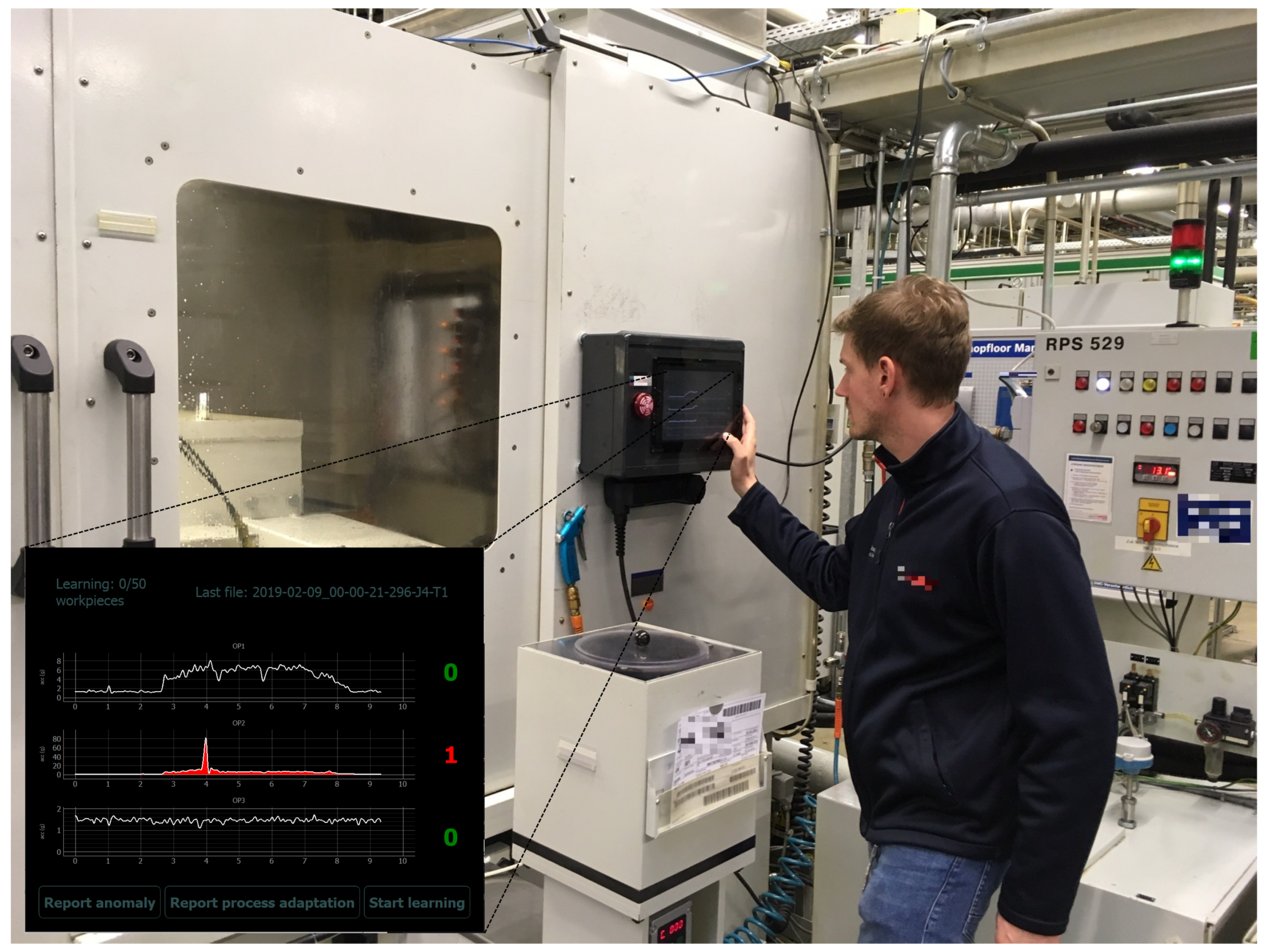
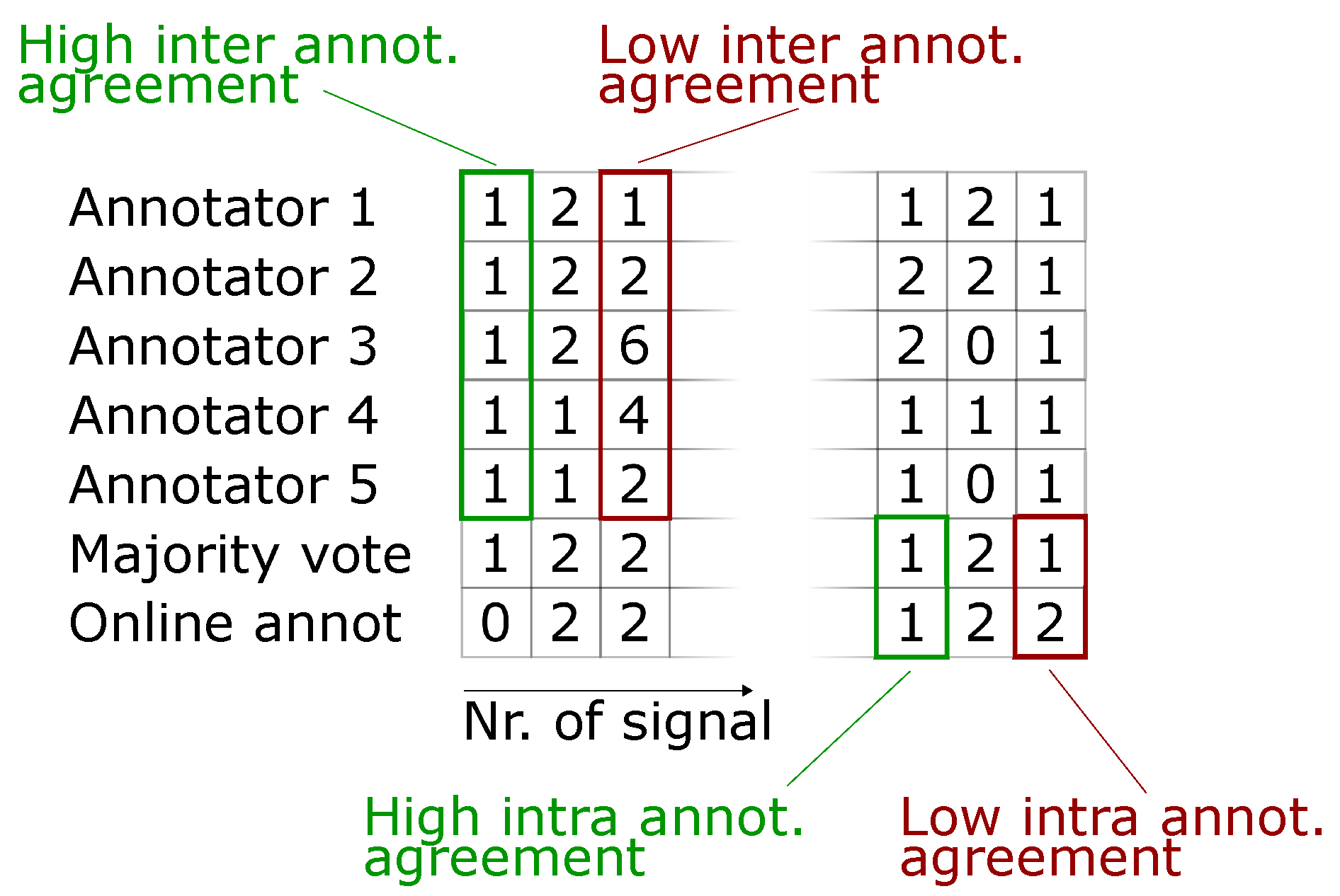
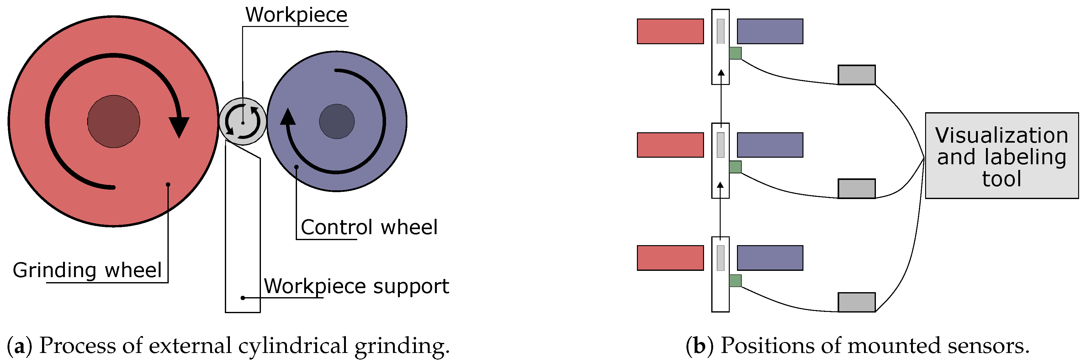
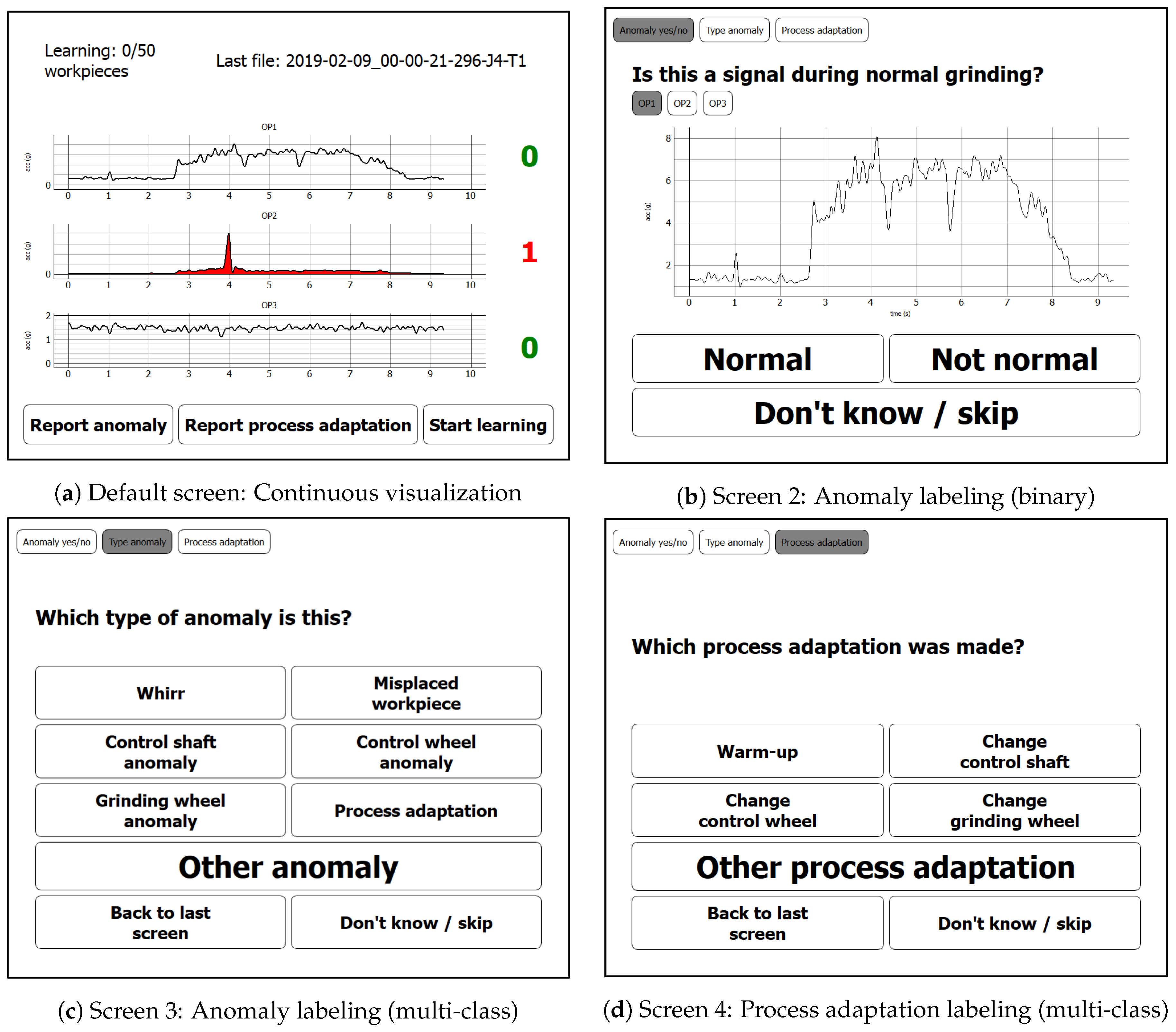
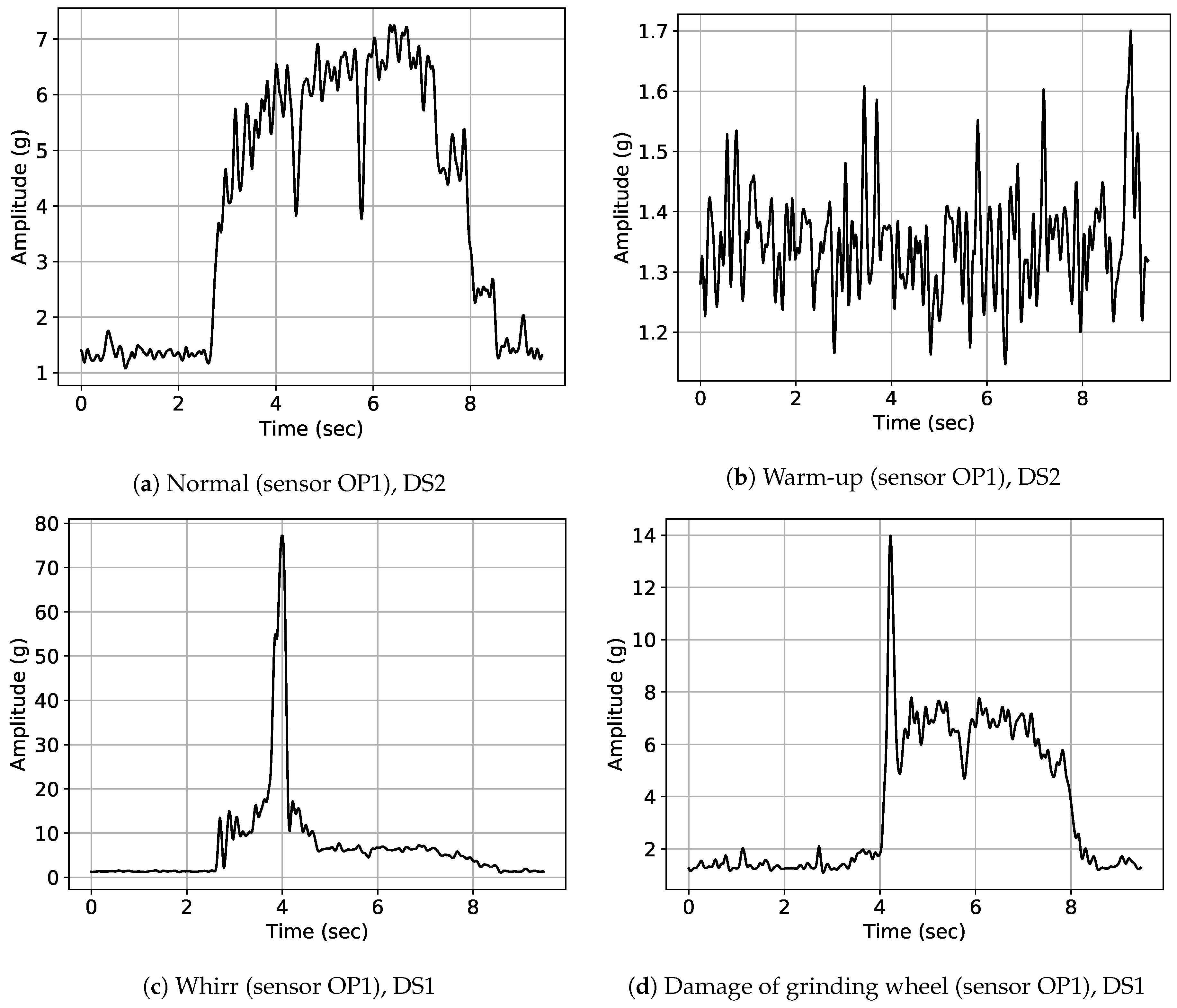
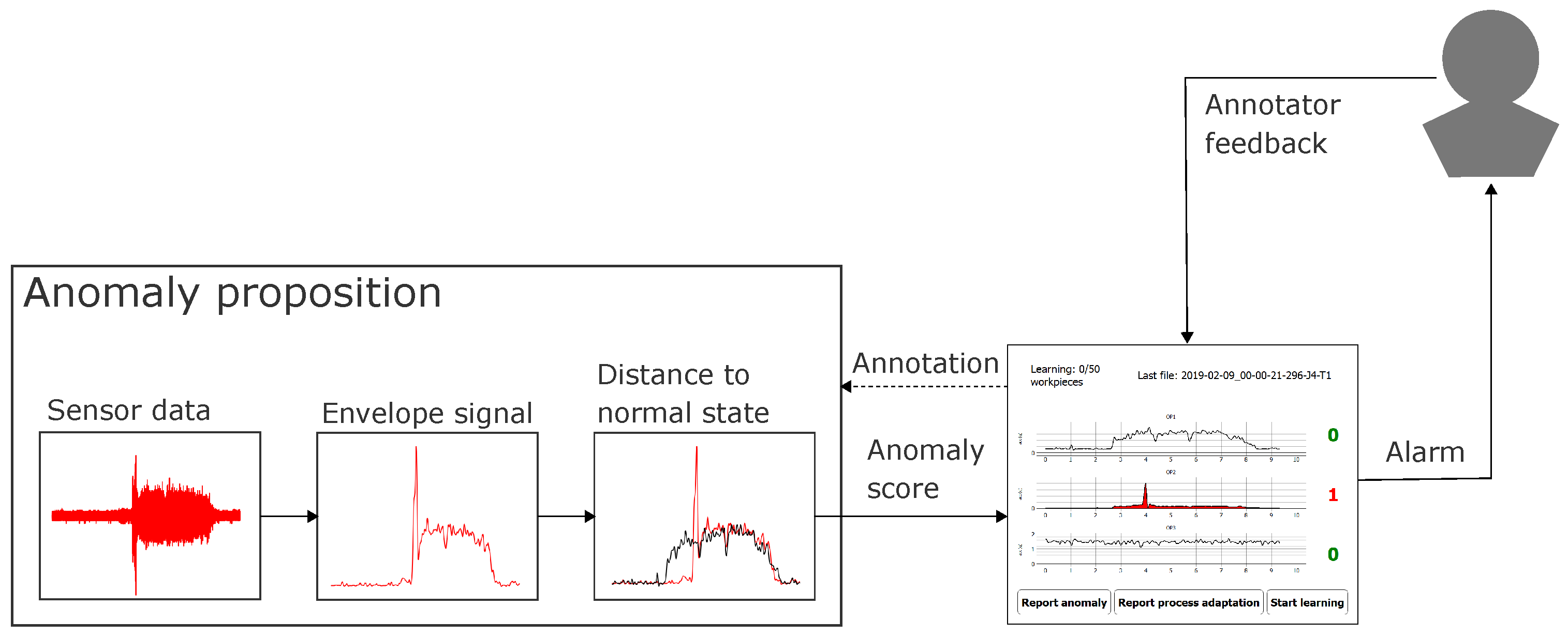
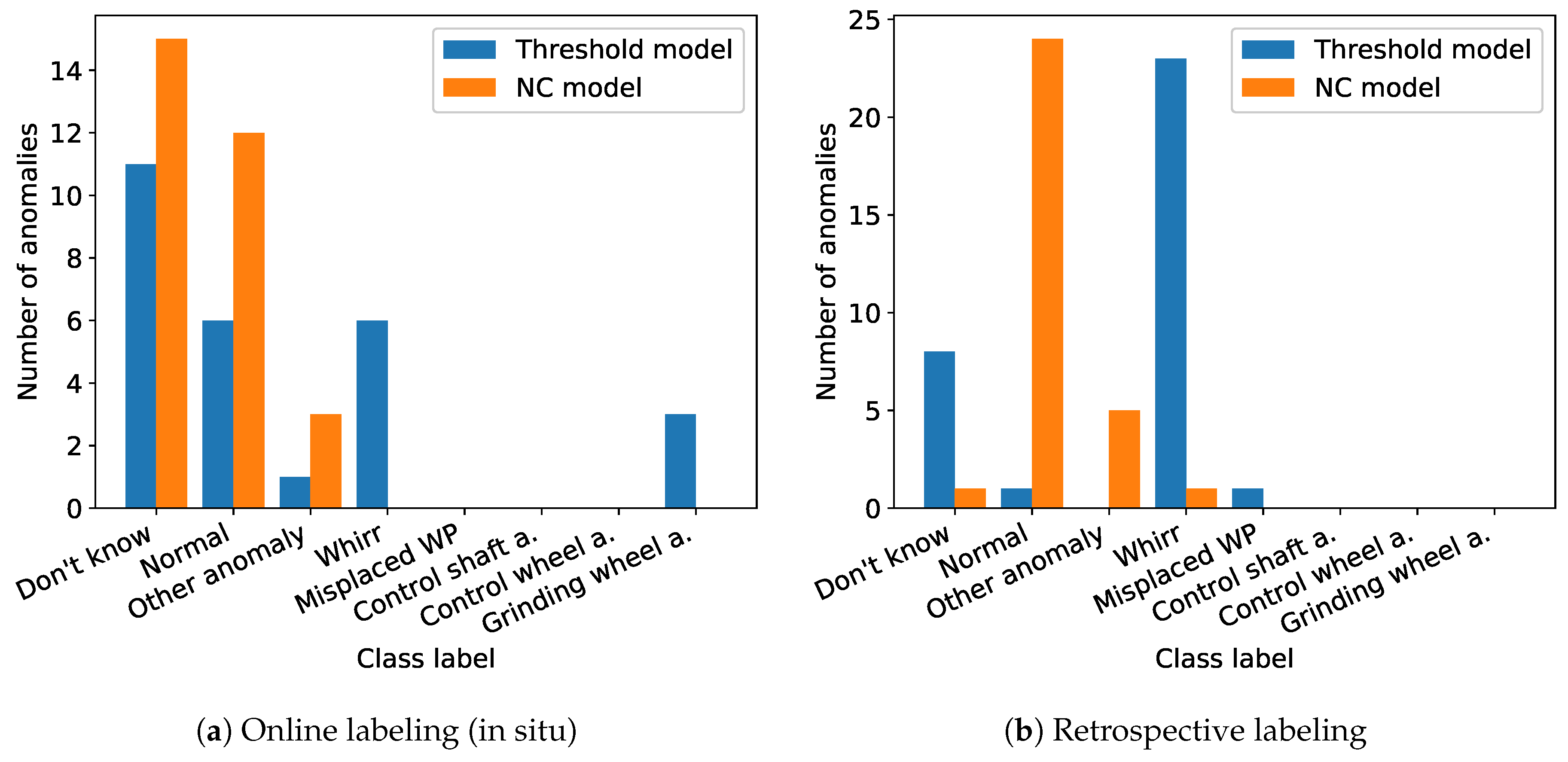
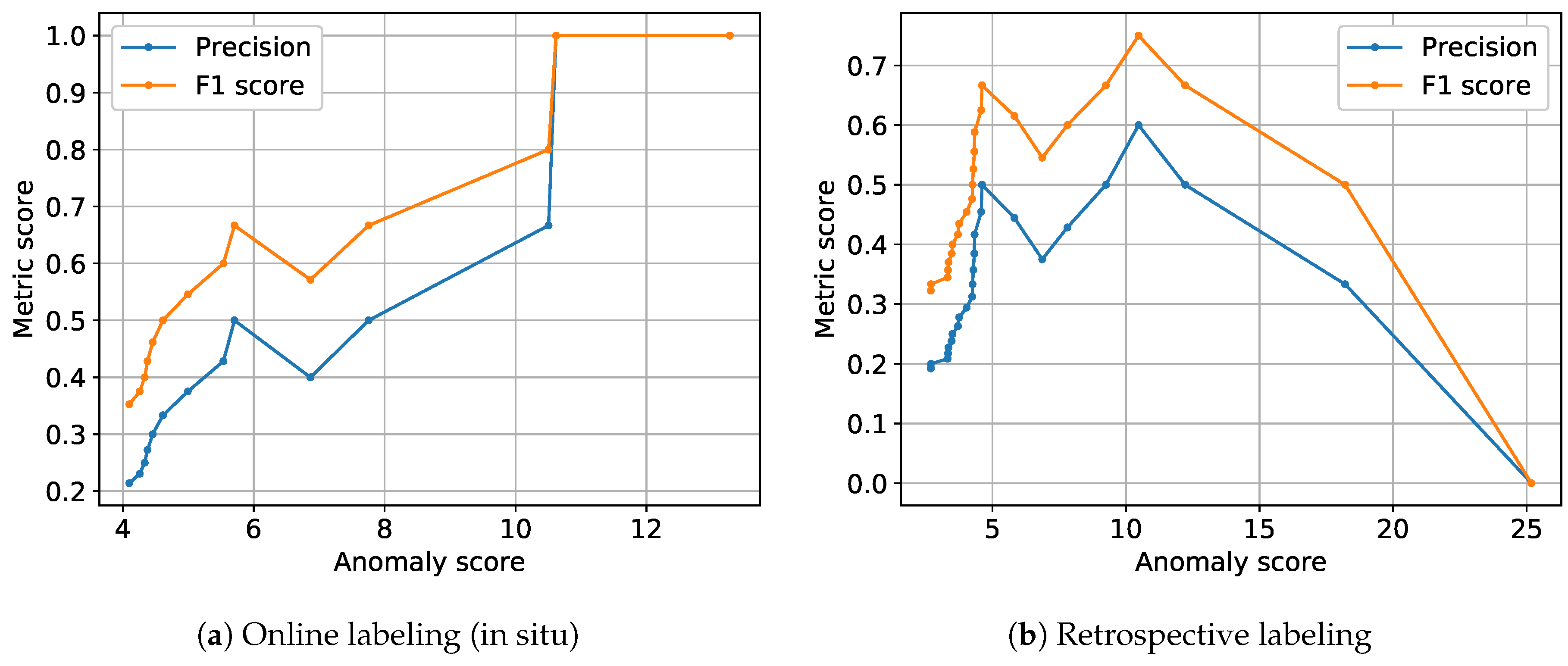
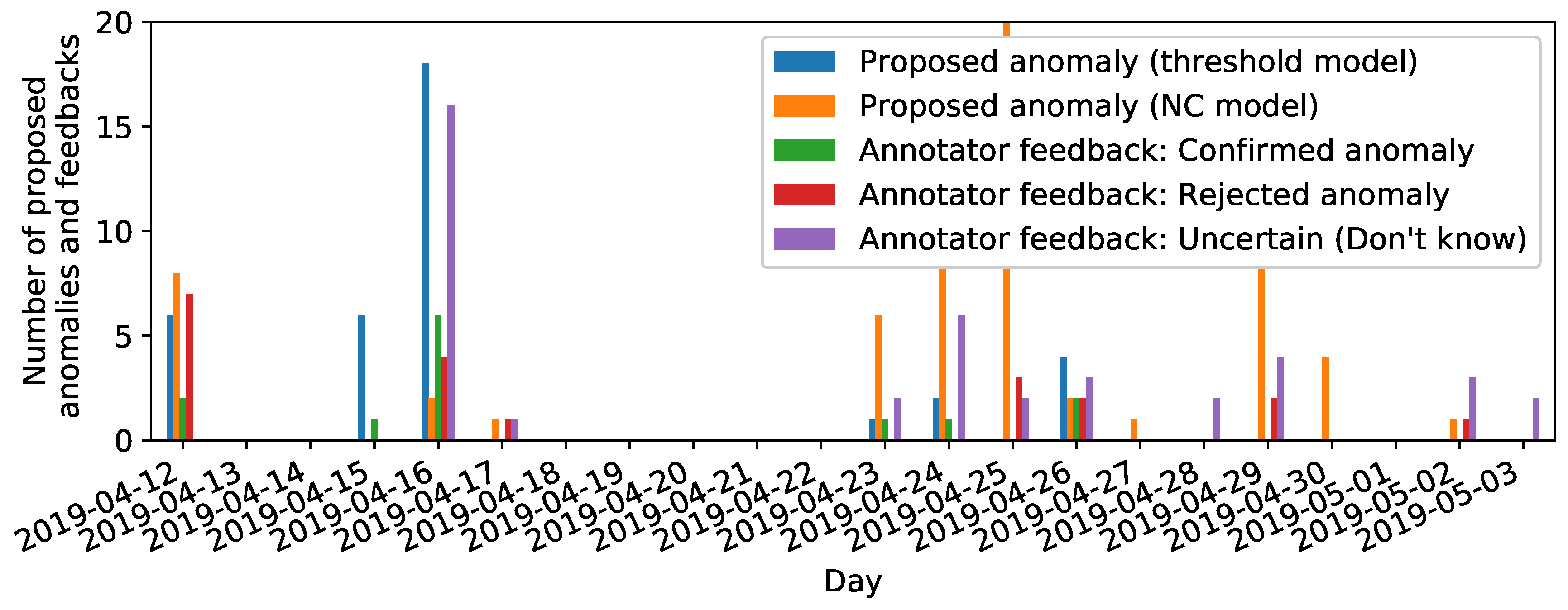
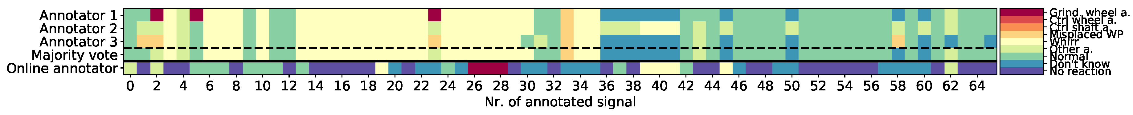
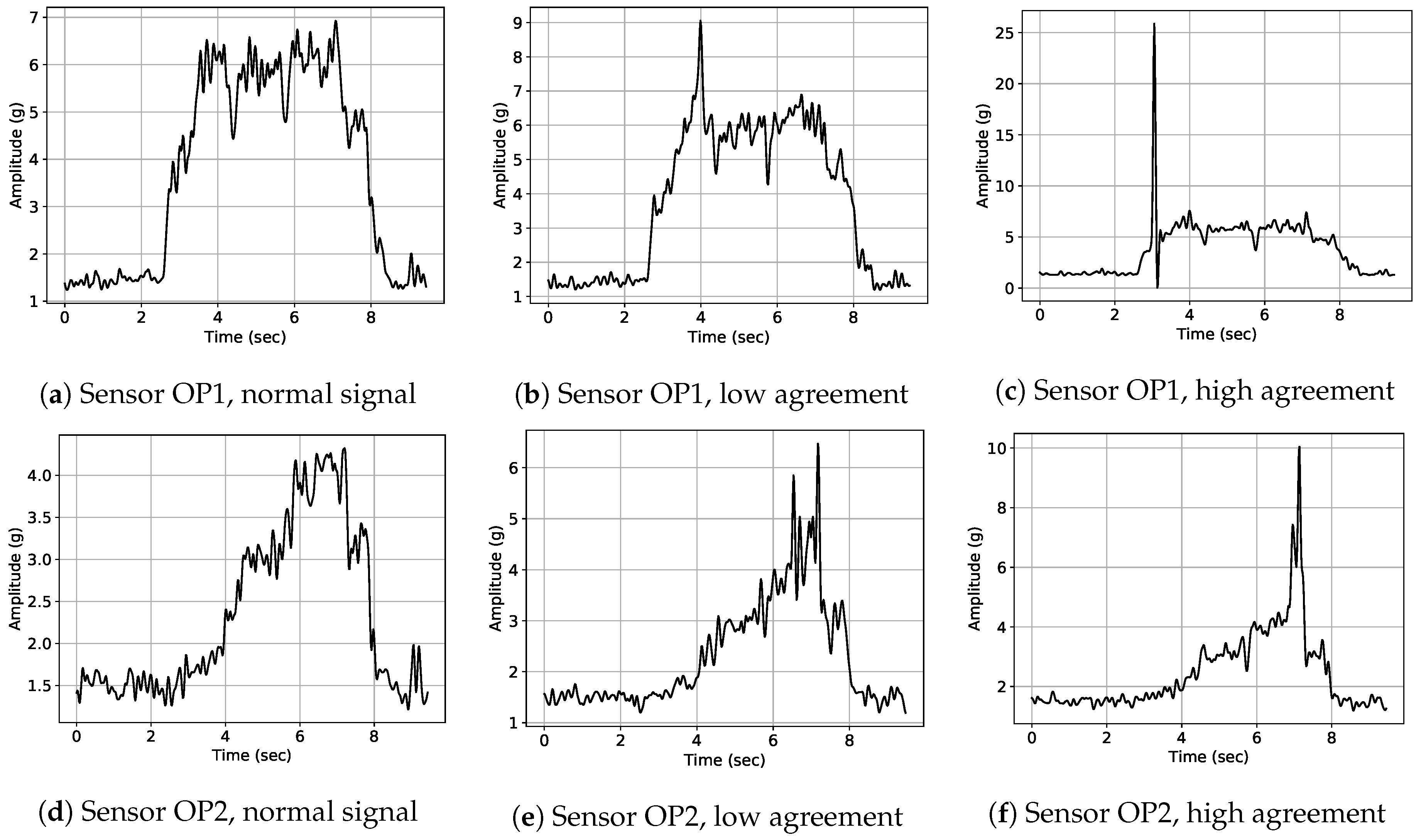
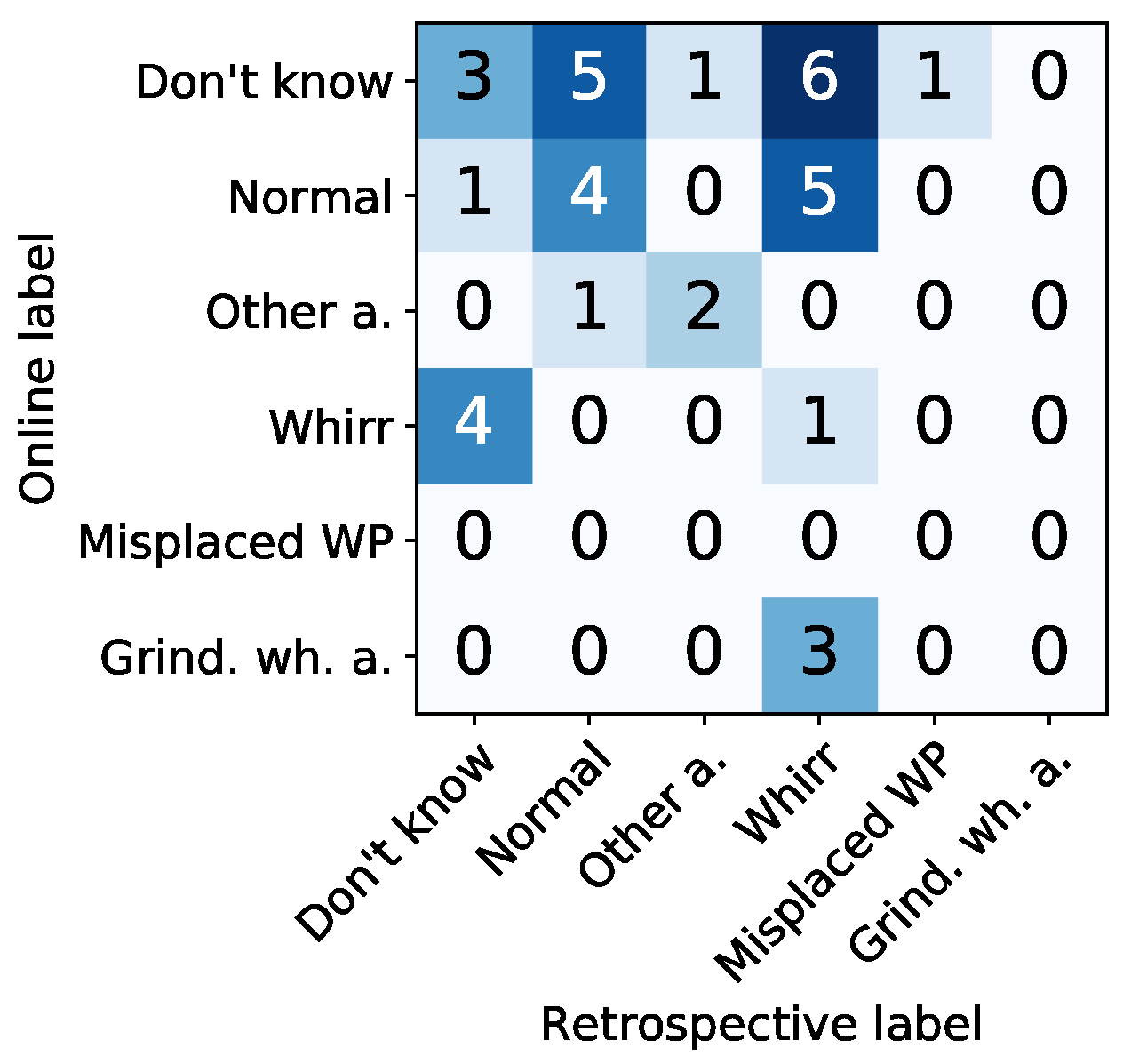
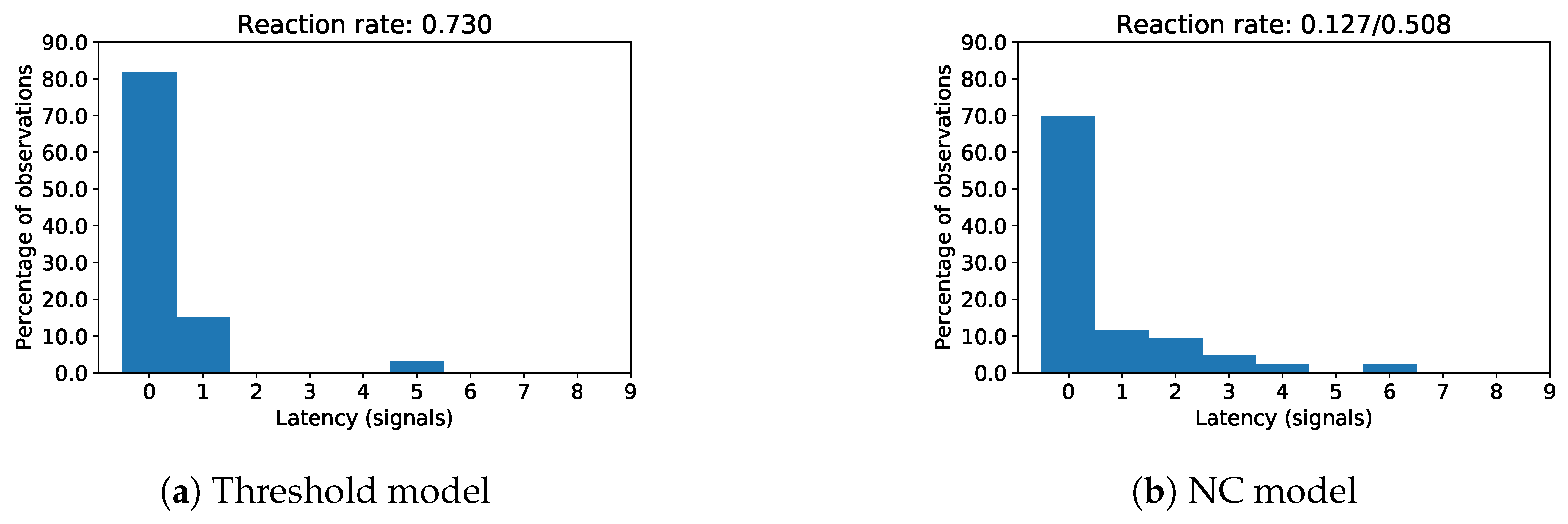
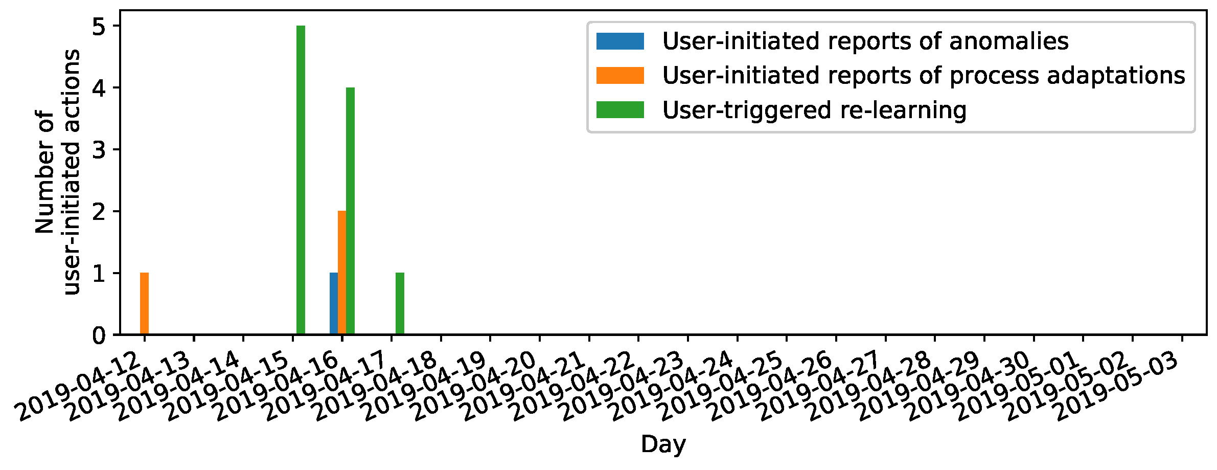
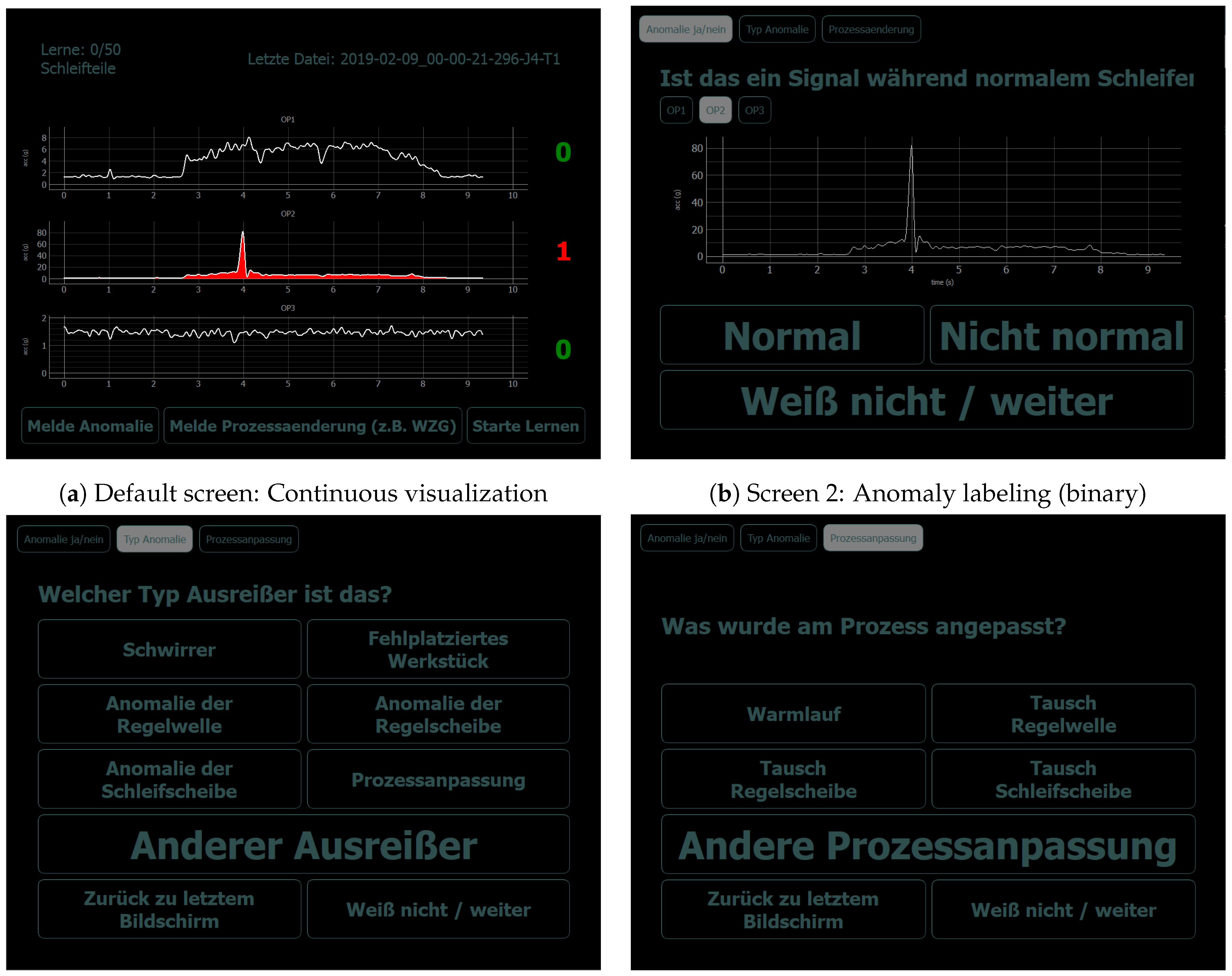
Table 1.
Comparison of anomaly detection models on data set DS1 (binary labels).
| Algorithm | F1 Score | Precision | Recall | Memory [kB] | Training Time [s] | Prediction Time [ms] |
|---|---|---|---|---|---|---|
| 1NN (ED) sup. | 99.85 | 99.85 | 99.85 | 8742 | 0.09 | 1.29 |
| NC (ED) | 99.75 | 99.75 | 99.75 | 23 | 0.05 | 0.05 |
| NC (ED+TI) | 99.80 | 99.80 | 99.80 | 23 | 0.78 | 0.47 |
| NC (DTW) | 99.20 | 99.22 | 99.19 | 21 | 1641.55 | 861.28 |
| NC (SDTW) | 99.30 | 99.30 | 99.30 | 21 | 205.99 | 1016.63 |
| LOF [45] | 52.32 | 88.45 | 47.25 | 170 | 0.05 | 0.03 |
| CBLOF [48] | 53.55 | 88.50 | 48.36 | 12 | 0.94 | 0.01 |
| IF [56] | 55.84 | 88.61 | 50.48 | 78 | 0.14 | 0.03 |
| kNN | 53.11 | 88.48 | 47.96 | 150 | 0.06 | 0.09 |
| MCD [39] | 67.45 | 89.37 | 62.24 | 19 | 0.61 | 0.01 |
| OCSVM [41] | 51.59 | 88.42 | 46.60 | 109 | 0.06 | 0.02 |
| HDBSCAN [28] | 96.26 | 96.61 | 96.47 | 599 | 0.20 | 0.01 |
| LODA [64] | 90.06 | 93.62 | 88.94 | 29 | 0.02 | 0.01 |
| HSTrees [61] | 96.43 | 96.75 | 96.62 | 278 | 6.31 | 5.12 |
| RSForest [60] | 96.15 | 96.31 | 96.31 | 304 | 4.82 | 5.10 |
| RSHash [65] | 95.92 | 96.12 | 96.11 | 1807 | 2.17 | 0.01 |
| xStream [58] | 96.25 | 96.45 | 96.42 | 246,994 | 13.00 | 8.04 |
Table 2.
Comparison of anomaly detection models on data set DS2 (binary labels).
| Algorithm | F1 Score | Precision | Recall | Memory [kB] | Training Time [s] | Prediction Time [ms] |
|---|---|---|---|---|---|---|
| 1NN (ED) sup. | 100.0 | 100.0 | 100.0 | 9675 | 0.06 | 1.44 |
| NC (ED) | 100.0 | 100.0 | 100.0 | 23 | 0.05 | 0.06 |
| NC (ED+TI) | 100.0 | 100.0 | 100.0 | 23 | 1.11 | 0.62 |
| NC (DTW) | 100.0 | 100.0 | 100.0 | 23 | 1676.78 | 785.73 |
| NC (SDTW) | 100.0 | 100.0 | 100.0 | 23 | 174.61 | 911.29 |
| LOF [45] | 99.41 | 99.60 | 99.32 | 190 | 0.05 | 0.04 |
| CBLOF [48] | 100.0 | 100.0 | 100.0 | 12 | 0.03 | 0.01 |
| IF [56] | 99.79 | 99.82 | 99.77 | 79 | 0.17 | 0.04 |
| kNN | 99.48 | 99.63 | 99.41 | 167 | 0.05 | 0.11 |
| MCD [39] | 99.75 | 99.79 | 99.73 | 20 | 0.66 | 0.01 |
| OCSVM [41] | 99.30 | 99.55 | 99.19 | 101 | 0.06 | 0.02 |
| HDBSCAN [28] | 99.98 | 100.0 | 99.01 | 669 | 0.35 | 0.01 |
| LODA [64] | 99.83 | 99.85 | 99.82 | 29 | 0.03 | 0.01 |
| HSTrees [61] | 99.65 | 99.68 | 99.68 | 278 | 6.75 | 5.08 |
| RSForest [60] | 99.71 | 99.73 | 99.73 | 304 | 4.95 | 5.14 |
| RSHash [65] | 100.0 | 100.0 | 100.0 | 2019 | 2.52 | 0.01 |
| xStream [58] | 99.81 | 99.82 | 99.82 | 224,335 | 15.17 | 9.35 |
© 2019 by the authors. Licensee MDPI, Basel, Switzerland. This article is an open access article distributed under the terms and conditions of the Creative Commons Attribution (CC BY) license (http://creativecommons.org/licenses/by/4.0/).
Share and Cite
MDPI and ACS Style
Reich, C.; Mansour, A.; Van Laerhoven, K. Collecting Labels for Rare Anomalies via Direct Human Feedback—An Industrial Application Study. Informatics 2019, 6, 38. https://doi.org/10.3390/informatics6030038
AMA Style
Reich C, Mansour A, Van Laerhoven K. Collecting Labels for Rare Anomalies via Direct Human Feedback—An Industrial Application Study. Informatics. 2019; 6(3):38. https://doi.org/10.3390/informatics6030038
Chicago/Turabian StyleReich, Christian, Ahmad Mansour, and Kristof Van Laerhoven. 2019. "Collecting Labels for Rare Anomalies via Direct Human Feedback—An Industrial Application Study" Informatics 6, no. 3: 38. https://doi.org/10.3390/informatics6030038
Note that from the first issue of 2016, this journal uses article numbers instead of page numbers. See further details here.