Image Super-Resolution Algorithm Based on an Improved Sparse Autoencoder


1
College of Engineering, Huaqiao University, No. 269, Chenghuabei Road, Quanzhou 362021, China
2
Department of Electronic Engineering, Shantou University, No. 243, Daxue Road, Shantou 515063, China
*
Author to whom correspondence should be addressed.
Information 2018, 9(1), 11; https://doi.org/10.3390/info9010011
Submission received: 4 December 2017
/
Revised: 28 December 2017
/
Accepted: 2 January 2018
/
Published: 5 January 2018
(This article belongs to the Section Information Processes)
Abstract
:Due to the limitations of the resolution of the imaging system and the influence of scene changes and other factors, sometimes only low-resolution images can be acquired, which cannot satisfy the practical application’s requirements. To improve the quality of low-resolution images, a novel super-resolution algorithm based on an improved sparse autoencoder is proposed. Firstly, in the training set preprocessing stage, the high- and low-resolution image training sets are constructed, respectively, by using high-frequency information of the training samples as the characterization, and then the zero-phase component analysis whitening technique is utilized to decorrelate the formed joint training set to reduce its redundancy. Secondly, a constructed sparse regularization term is added to the cost function of the traditional sparse autoencoder to further strengthen the sparseness constraint on the hidden layer. Finally, in the dictionary learning stage, the improved sparse autoencoder is adopted to achieve unsupervised dictionary learning to improve the accuracy and stability of the dictionary. Experimental results validate that the proposed algorithm outperforms the existing algorithms both in terms of the subjective visual perception and the objective evaluation indices, including the peak signal-to-noise ratio and the structural similarity measure.
1. Introduction
In the remote sensing, medical, military, and other fields, the acquisition of high-resolution (HR) images is of great significance. Image super-resolution (SR) is a technique that uses signal processing approaches to enhance the spatial resolution of the image. Its key is to add some additional information into the process of image reconstruction to compensate for the loss of detail information due to image degradation, so that it could reconstruct a clear HR image from a low-resolution (LR) image [1]. The SR algorithm based on dictionary learning utilizes the characteristic that the natural images have a sparse representation under a specific dictionary, and applies the dictionary learning method to construct the dictionaries which can represent image patches sparsely, and then some additional information can be obtained to improve the quality of the reconstructed image [2].
The purpose of dictionary learning is to decompose the data matrix into a dictionary matrix and a representation matrix, so it is also known as “matrix factorization”. In the late 1990s, dictionary learning began to be applied in vision [3] and information retrieval [4]. At present, dictionary learning has been widely used to solve inverse problems in image processing, such as image denoising [5], image inpainting [6], color image restoration [7], inverse half toning [8], and even medical image reconstruction [9,10].
The dictionary learning methods can be divided into two categories, the mathematical transformation-based methods and the learning-based methods. The wavelet transform (WT) dictionary and the overcomplete discrete cosine transform (DCT) dictionary belong to the mathematical transformation-based methods. Dattatray et al. [11] and Dabbaghchian et al. [12] learned face image samples by using WT and DCT, respectively, and applied the learned mathematical transformation-based dictionary to face recognition. Although the mathematical transformation-based dictionary is simple and easy to implement in the case of representing the signal sparsely, the expression of the signal is single and without self-adaptability. However, the learning-based dictionary has a relatively strong adaptive ability, which can better adapt to different image data. The method of optimal directions (MOD) proposed by Engan et al. [13] is the originator of the learning-based dictionary, and its dictionary update approach is simple, but its convergence speed is very slow. Aharon et al. [14] proposed the K-SVD algorithm, which is the most popular dictionary learning method. The algorithm learned the dictionary under the strict sparse condition by giving a set of training signals so that each signal has the best representation. Moreover, the convergence speed of the K-SVD algorithm is faster than that of the MOD algorithm. Mairal et al. [15] proposed an online dictionary learning algorithm that has high training speed and is suitable for the processing of special signals, such as video signals and voice signals. With the development of machine learning, the models of unsupervised learning, such as neural networks or deep learning, provide some new ideas for dictionary learning. In [16], the dictionary learning method was proposed by using some models including deep belief networks and a stacked autoencoder.
We apply a sparse autoencoder (SAE) to the SR algorithm and propose two image SR algorithms. The main contributions of this paper are summarized as follows:
- A novel training set preprocessing method is proposed. By regarding the high-frequency information of the image as the characterization, we construct the HR and LR image training sets with different methods, and then apply the zero-phase component analysis (ZCA) whitening method to reduce the redundancy of the joint training set to improve the learning efficiency of the SAE.
- An improved SAE (ISAE) is proposed to boost the accuracy and stability of the dictionary. A new sparse regularization term related to the hidden layer is introduced into the cost function of the traditional SAE to further strengthen the sparseness constraint on the hidden layer, so that the number of hidden units whose average activation is close to zero is as many as possible.
- The SR algorithm based on the SAE (SRSAE) and the SR algorithm based on the ISAE (SRISAE) are proposed. The SAE is employed to achieve unsupervised dictionary learning, and then by applying this unsupervised dictionary learning method to the SR algorithm based on sparse representation, the SRSAE can be constructed. By replacing the SAE with the ISAE, the SRISAE can be obtained using the same procedure described above.
The remainder of this paper is organized as follows. Section 2 introduces the related works. Section 3 presents the basic theory of the image SR algorithm based on dictionary learning. Section 4 describes the proposed algorithm, including the training set preprocessing method, the unsupervised dictionary learning model based on the ISAE, and the specific overall flow of our algorithm. In Section 5, some experimental results are shown to verify the effectiveness of our algorithm. Section 6 concludes the paper.
2. Related Works
Dictionary learning can achieve better sparse representation and discriminative information through the custom design for the dictionary, which can improve the quality of the reconstructed image. In recent years, the SR algorithm based on dictionary learning has attracted a large number of scholars’ attention and has become one of the most important research directions of the single-image SR algorithm.
Yang et al. [17] regarded the image library consisting of a large number of HR images as training samples, and generated the corresponding LR images training samples by down-sampling the HR images. Then, the joint dictionary training algorithm was used to train the HR and LR images so that the sparse representation coefficients of the LR image patches were similar to those of the corresponding HR image patches. Consequently, the HR image patches could be generated approximately through the sparse representation coefficients of LR image patches and the HR dictionary. Although the algorithm can obtain sufficient additional information to restore some high-frequency detail information, the accuracy and stability of the additional information cannot be guaranteed when the training image library cannot provide image patches similar to the image to be reconstructed. Zeyde et al. [18] improved Yang’s algorithm [17] through applying the K-SVD approach and the pseudo-inverse approach to train the LR dictionary and the HR dictionary, respectively. Compared with Yang’s algorithm, this algorithm improves the quality of the reconstructed image and reduces image artifacts. To avoid a large number of image training samples and obtain more accurate prior knowledge, Jing et al. [19] proposed an SR algorithm based on multi-task dictionary learning, which learned a multiple-examples-aided redundant dictionary from different classes of samples classified by the K-Means approach to provide a more suitable dictionary for the reconstruction of each sample. The algorithm can not only reduce the computational complexity caused by the large dictionary, but also has good reconstruction performance. In [20], the SR algorithm based on the K-SVD method and semi-coupled dictionary learning was proposed to solve the time-consumption problem in dictionary learning. The K-SVD algorithm was applied to train the dictionary pair in the semi-coupled dictionary learning model, which not only reduces the dictionary learning time, but also improves the quality of the reconstructed image. Zhang et al. [21] proposed a single-image SR algorithm based on label consistency K-SVD (LC-KSVD). The algorithm introduced a new label consistency constraint called “discriminative sparse code error” into the K-SVD objective function, which made the learned dictionary possess both good representation and discrimination ability. Accordingly, the reconstruction performance and the robustness of this algorithm become better than that of the K-SVD algorithm.
For unsupervised dictionary learning, such as neural networks, Zhang et al. [22] learned a feature dictionary from a large number of unlabeled remote sensing images by using the SAE, and retrieved the remote sensing images through the learned dictionary and a convolutional neural network. The algorithm effectively improves the speed and accuracy of remote sensing image retrieval.
At present, the research on applying dictionary learning based on a neural network model to an image SR algorithm is still relatively rare. Inspired by the literature [22], an improved SAE is proposed for unsupervised dictionary learning to enhance the accuracy and stability of the dictionary, and it is applied to the SR algorithm to improve the quality of the reconstructed images.
3. Image SR Algorithm Based on Dictionary Learning
We define as the HR image, as the LR image, as the down-sampling operator, and as the additive white noise. Then, the degradation model from the HR image to the LR image can be defined as,
Assuming that there is an overcomplete HR dictionary and an LR dictionary , and the HR and LR images have the same sparse representation coefficients [2], then the HR image can be reconstructed by combining HR dictionary with sparse representation coefficients ,
Since the LR image is known, its sparse coefficients can be solved by combining LR dictionary with the LR image . The model of the solution is as follows,
In general, the optimization of Equation (3) is an NP-hard problem. Supposing that the sparse representation coefficients are sparse enough, solving the -norm minimization problem can be replaced by solving the -norm minimization problem [23]. Then, the Lagrange multiplier is used for equivalent conversion to obtain the following sparse coding function,
where is a parameter used to balance the sparsity of the solution and the fidelity of the LR image . The sparse coefficients can be obtained by solving Equation (4), and then the HR image can be reconstructed.
4. Proposed Algorithm
4.1. Training Set Preprocessing Method
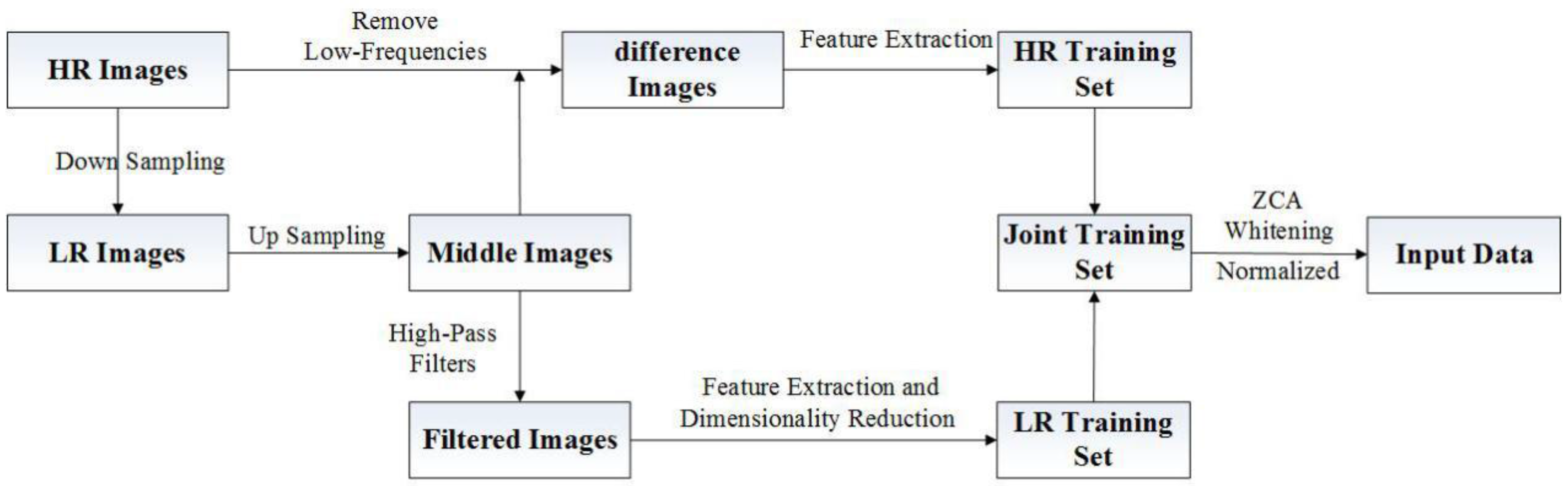
The sample images used to construct the training sets contain 91 HR images derived from literature [2]. Let represent the HR images. Then, the corresponding LR images can be obtained by down-sampling these HR images using the degradation model shown as Equation (1), and the corresponding middle images of the same size as the HR images can be obtained by up-sampling these LR images with Bicubic interpolation.
Construct the HR training set. To train the characterization of the relationship between the HR patches and their corresponding LR patches in the edge and the texture, the HR images are subtracted from the middle images to remove their low-frequency information, that is, the difference images can be obtained via . Then, the HR training set can be obtained by performing feature extraction on the difference images .
Construct the LR training set. To extract the local characterization corresponding to their high-frequency information, the middle images , which are the enlarged images from the LR images, are filtered by using high-pass filters, that is, , (where the symbol * indicates a convolution operation). These high-pass filters can be gradient filters or Laplacian filters. Then, feature extraction is performed on the filtered images, and the LR training set can be obtained. Considering that the dimension of increases as the middle images are filtered with high-pass filters, the sparse principal component analysis (SPCA) [24] algorithm is employed to reduce the dimension of to reduce the computational complexity of the dictionary learning. The SPCA algorithm, which is based on the PCA algorithm, introduces a new constraint term to find the sparse principal components which can be represented by the linear combination of the smallest but most representative variables. In this way, it can not only reduce the time of dimensionality reduction, but also obtain more accurate principal components and improve the ability of explanation and analysis. After reducing the dimension of , the LR training set can be expressed as .
In summary, we can obtain the joint training set by combining the HR training set with the LR training set .
Zero-phase component analysis (ZCA) whitening. Due to the strong correlation that exists between adjacent pixels in the image, the ZCA whitening technology [25] is adopted to eliminate the redundancy of the joint training set .
Through ZCA whitening, the correlation between the features of each image patch in the training set is reduced, and the features of all the image patches have the same variance. We define as the HR training set, as the LR training set, and as the corresponding joint training set. The main process of ZCA whitening is listed as follows.
Firstly, calculate the eigenvector matrix through decomposing the covariance matrix of the joint training set by Singular Value Decomposition (SVD). For matrix , it possesses the orthogonality property and satisfies . Secondly, rotate the features according to . Thirdly, utilize the PCA whitening approach to process the rotated features so that each feature has unit variance, that is, , where is the value of the diagonal element of the covariance matrix of . Finally, left multiply the matrix with to obtain the ZCA whitening features ,
where , the joint training set processed by the ZCA whitening is . In the ZCA whitening stage, the data dimension will be maintained and no longer reduced. In addition, since the range of input samples of the SAE must be scaled to , the training set needs to be normalized.
The proposed training set preprocessing method can not only effectively reduce the computational complexity of the SAE to save the training time, but also reduce the correlation between the features, which lays the foundation for dictionary learning. The framework of the proposed training set preprocessing method is illustrated as Figure 1.
4.2. Unsupervised Dictionary Learning Model Based on ISAE
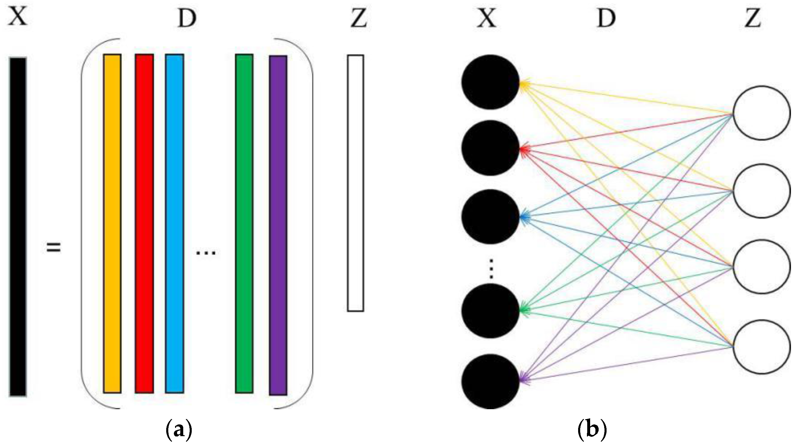
The traditional dictionary matrix can be seen as consisting of multiple atoms, where each column of the matrix corresponds to an atom. In [16], an unsupervised dictionary learning method is performed using a deep neural network, and the column of the dictionary is treated as the connection between the input layer and the presentation layer. Thus, the updated connection weights are equivalent to the learned dictionary. The relationship between dictionary learning and the neural network representation is shown as Figure 2. In Figure 2, stands for the data, represents a basis which also called a ‘dictionary‘ and the columns of are called ‘atoms’, and indicates the representing of .
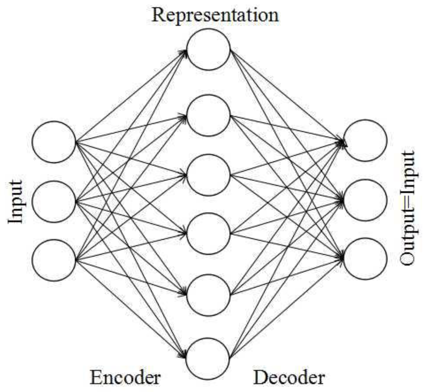
In this paper, the SAE is employed to achieve unsupervised dictionary learning. The SAE is a traditional feedforward neural network including an input layer, a hidden layer, and an output layer. In this model, the number of hidden units is greater than that of the input units, and its structure is illustrated as Figure 3. The main reasons why we choose the SAE for dictionary learning include, on the one hand, that the SAE can automatically learn more sparse and compact data characteristics from unlabeled data on the condition that the output is approximately equal to the original input. On the other hand, the number of hidden units is equivalent to the dictionary dimension, so the SAE with far more hidden units than input units can guarantee that the learned dictionary has the overcomplete property.
The SAE consists of an encoder and a decoder. The encoder maps the input vector to the hidden layer in a certain way by means of a nonlinear mapping function,
where , , is the weight matrix of the input layer to the hidden layer, is the bias vector of the input layer, , and is the activate function. The decoder is responsible for mapping the hidden layer to the output layer . The output layer has the same number of units as the input layer, and the mapping relationship is as follows,
where , is the weight matrix of the hidden layer to the output layer, and its value is the same as the transpose of , and is the bias vector of the hidden layer, , where the parameters can be expressed as by merging and .
The SAE minimizes the reconstruction error between input and output by adjusting the parameter . In general, the mean squared error (MSE) is used as its cost function, and a weighted attenuation term is added to the cost function to reduce the magnitude of the weights and prevent overfitting. Moreover, to ensure that the hidden units are inactive most of the time, the regularization term used to constrain the sparsity of the hidden layer is added to the cost function. Assuming that its input data is (where the data from to belongs to the HR training set, and the data from to belongs to the LR training set), and its output data is , the cost function of the traditional SAE can be expressed as,
where and are the number of samples in the HR and LR training sets, respectively, is the input data, is the output data, is the number of layers, is the number of units in layer , is the average activation of the hidden unit , is the expected activation whose value is set to close to 0, and and are the regularization parameters. In this paper, the kullbackleibler (KL) divergence is utilized to penalize for significant deviation from , and its expression is as follows,
Combined with the SR theory based on dictionary learning and the SAE model, a more accurate dictionary can be generated as long as the sparsity of the hidden layer can be further improved. Consequently, to ensure that the number of hidden units whose average activation is close to zero is as many as possible, the norm is adopted to strengthen the sparseness constraint on the hidden layer in this paper, and then the cost function of ISAE can be expressed as,
where is a regularization parameter used to adjust the constructed sparse regularization term, and is the activation matrix of all the hidden units, whose expression is as follows,
where is the activation value of unit in layer , is the weight associated with the connection between unit in layer and unit in layer , and is the bias vector associated with unit in layer .
The selection of the activation function. The Sigmoid function can scale the input data to , which satisfies the requirement of SAE. In addition, the data of the Sigmoid function is not easy to diverge in the process of transmission, and its derivation is simple to calculate. Hence, we select the Sigmoid function as the activation function in the encoding stage, and its corresponding expression is as follows:
Although the Sigmoid function can improve the performance of the SAE to a certain extent, the SAE has an inherent drawback that the range of its input data must be scaled to . To solve the problem of data scaling, in the decoding stage, we use a linear decoder, that is, ; accordingly, the residuals can be calculated more accurately to improve the accuracy of the dictionary [26].
To minimize the improved cost function, the gradient descent (GD) method [27] is adopted to update the weights and the bias vectors, and then the connection weights from the input layer to the hidden layer can be obtained. According to the relationship between dictionary learning and neural network representation shown as Figure 2, the learned dictionary in our algorithm is equivalent to the transpose of , that is, . Consequently, the dictionary is expressed as , where , is the dictionary dimension, , and the HR dictionary and LR dictionary can be written as and , respectively. So, the dictionary pair obtained by applying the ISAE can be expressed as .
4.3. The Overall Flow of the Proposed Algorithm
The overall flow of the proposed SR algorithm is illustrated as Algorithm 1.
| Algorithm 1: Proposed SR algorithm. |
| Input: an LR image to be reconstructed, the HR sample images for dictionary learning. Step 1: obtain the LR images by down-sampling the HR images , and then obtain the middle images of the same size as the HR images by up-sampling the LR images with Bicubic interpolation. Step 2: obtain the HR and LR joint training set through preprocessing the HR images , the LR images , and the middle images by applying the proposed training set preprocessing method. Step 3: generate the HR dictionary and LR dictionary by utilizing the ISAE to learn the joint training set . Step 4: calculate the sparse representation coefficients of the LR image to be reconstructed under the learned LR dictionary by using the feature-sign search (FSS) algorithm [28]. Step 5: reconstruct the HR image via . Step 6: obtain the final reconstructed HR image by compensating for with the global error compensation model based on the weighted guided filter [29]. Output: HR image . |
5. Experiments
To verify the effectiveness of the proposed algorithm, a series of simulation experiments were carried out. Those experiments are implemented in MATLAB 2014a software installed on a 64-bit Windows Operating System, which runs on an Inter(R) Core(TM) i7-7700K CPU @ 4.20GHz with 16 G of memory. The performance of the SR algorithms is evaluated subjectively and objectively. In the subjective evaluation, details such as the edge and texture of the reconstructed images are analyzed. In the objective evaluation, we calculate two indices, the peak signal-to-noise ratio (PSNR) [30] and the structural similarity measure (SSIM) [31], based on the reconstructed images and the original reference HR images. The higher the PSNR value is, the better the quality of the reconstructed image is and the better the performance of the corresponding SR algorithm is. The closer the SSIM value is to 1, the more similar the reconstructed image is to the original image and the better the performance of the corresponding SR algorithm is. In our experiments, the maximum PSNR or SSIM is highlighted in bold type. The PSNR and the SSIM are calculated as follows,
where is the reconstructed HR image, is the original HR image, and are the rows and columns of the HR image, respectively, and are the mean of and , respectively, and are the variance of and , respectively, is the co-variance, and and are the constants.
5.1. Samples and Settings
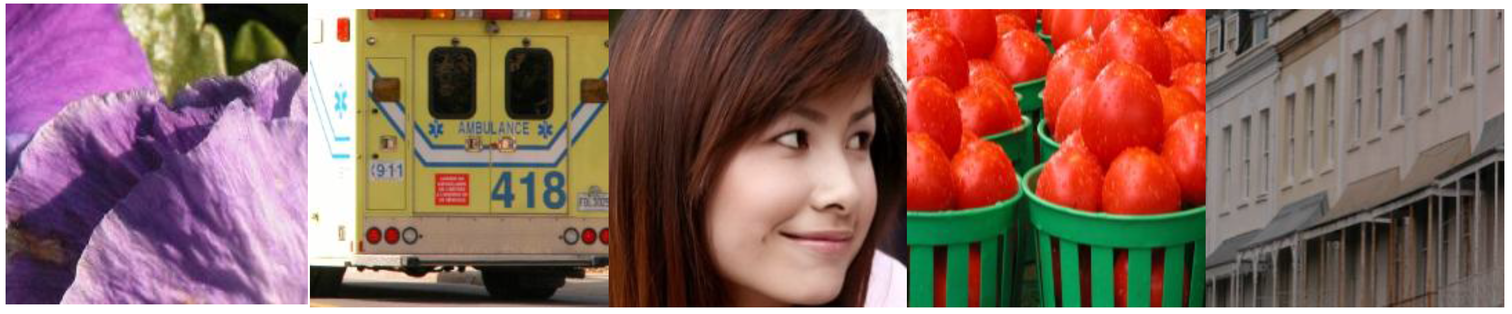
In the dictionary learning stage, the training samples used in the experiments are derived from the training set in literature [2], and include natural images such as landscapes, people, and buildings. Some of the samples are shown in Figure 4. To ensure the objectivity of the experiments, the test images used in the experiments are selected from three image sets: Set5 [32], Set14 [33], and B100, where B100 includes 100 images selected from BSDS300 [33]. To quantitatively evaluate the quality of the reconstructed images, these test images are regarded as the HR reference images, and the LR images to be reconstructed are obtained through down-sampling these HR images. The sampling factor is assigned the value 3. In the training set preprocessing stage, we set , that is, four high-pass filters are used, , , , and . In the stage of dictionary learning, the parameters related to the cost function are set as follows: , , , . In the process of image reconstruction, the image patch size is set to .
5.2. Experimental Results
5.2.1. Analyze the Influence of Different Number of Hidden Units on the Reconstructed Images
In order to discuss the influence of different numbers of hidden units on the performance of the proposed algorithm, the dictionary dimensions are set to 256, 512, 1024, and 2048, respectively. In this way, the optimal number of hidden units can be determined. In this experiment, the images in Set5 are selected as the test images.
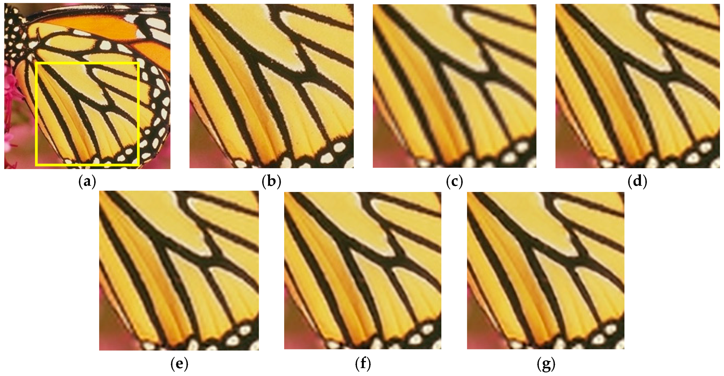
Figure 5 shows the reconstructed results of Butterfly using the dictionaries with different numbers of hidden units from subjective visual perception. To better compare and analyze the performance of different SR algorithms, we enlarge the area with more details, which is highlighted with a yellow rectangle in the corresponding image. It can be seen from Figure 5 that the reconstructed image is still vague and there are obvious jagged effects at the edge when the number of hidden units is 256. When the number of hidden units is 512 and 1024, the texture and edge of the reconstructed images is gradually improved, the artifacts are fewer and fewer, and the reconstructed images become clearer and clearer. However, when the number reaches 2048, there is no significant improvement for the quality of the reconstructed image, but more time is spent on dictionary learning. Table 1 lists the PSNR and SSIM values of the reconstructed images using the dictionaries with different numbers of hidden units for Set5. From Table 1, we can see that the PSNR and SSIM values of the reconstructed images in Set5 gradually increase with the increase of the number of hidden units. However, as the number of hidden units increases to 2048, the PSNR and SSIM values of the reconstructed images corresponding to most of the images in Set5 decrease. Therefore, combining with the results in Figure 5 and Table 1, we set 1024 as the optimal number of hidden units, that is, the dictionary dimension is set to 1024.
5.2.2. Analyze the Effectiveness of Dictionary Learning Based on SAE or ISAE
In this experiment, the test images are derived from set5, set14, and BSD100, and the number of hidden units is set to 1024. The purpose of this experiment is to verify that it is effective to apply the SAE or the ISAE for dictionary learning. Consequently, we compare Bicubic interpolation with the proposed SRSAE and SRISAE algorithms.
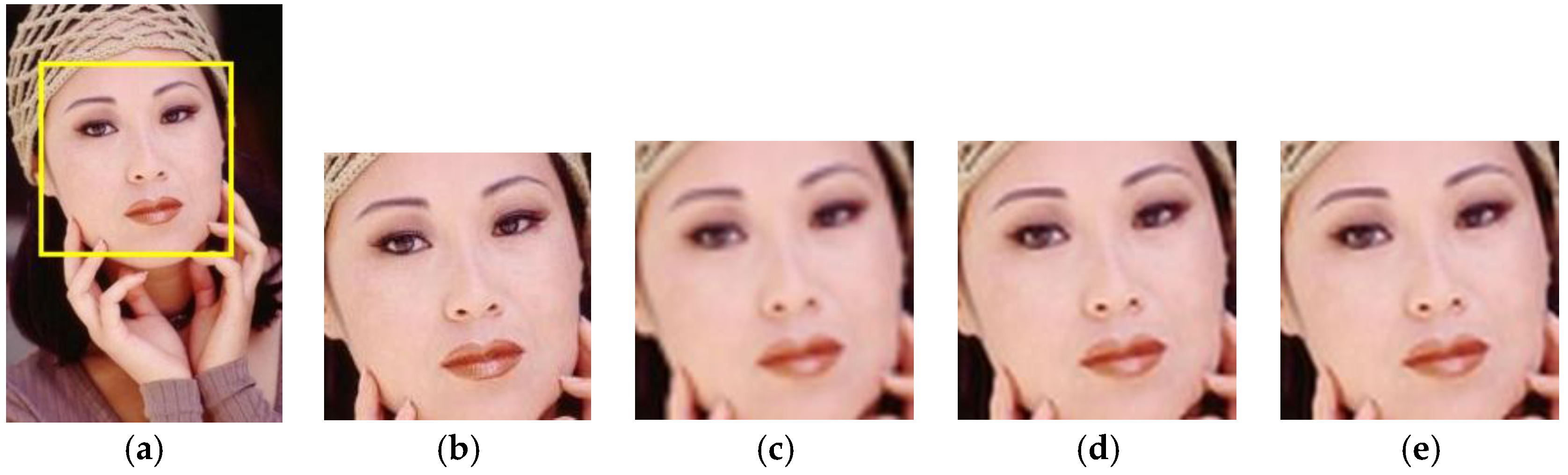
Figure 6 shows the reconstructed results of Woman with these three SR algorithms from subjective visual perception. We can see that the details of the reconstructed images obtained by the SRSAE and SRISAE algorithms are significantly more abundant than the Bicubic algorithm. Moreover, compared with the SRSAE algorithm, a lot of artifacts in the reconstructed images obtained by SRISAE are reduced; for instance, the woman’s face is clearer. Table 2 lists the average PSNR and SSIM values of these three algorithms for the test image sets Set5, Set14, and BSD100. It can be seen from Table 2 that the average PSNR and SSIM values of the SRSAE algorithm are much larger than those of the Bicubic algorithm and that the performance of the SRISAE algorithm is better than that of the SRSAE algorithm.
5.2.3. Analyze the Performance of Different SR Algorithms on Images Sets
To further verify the performance of the proposed SRISAE algorithm, it is compared with eight SR algorithms, including Super Resolution with L1 Regression (L1SR) [2], Single Image Super Resolution (SISR) [18], Anchored Neighborhood Regression (ANR), Neighbor Embedding with Least Squares (NE + LS), Neighbor Embedding with Non-Negative Least Squares (NE + NNLS), and Neighbor Embedding with Locally Linear Embedding (NE + LLE), mentioned in literature [34], Adjusted Anchored Neighborhood Regression (A+)(16 atoms) [35], and improved Super Resolution based on Sparse representation(ISPSR) [29]. The eight test images are selected from Set5 and Set14 in this experiment.
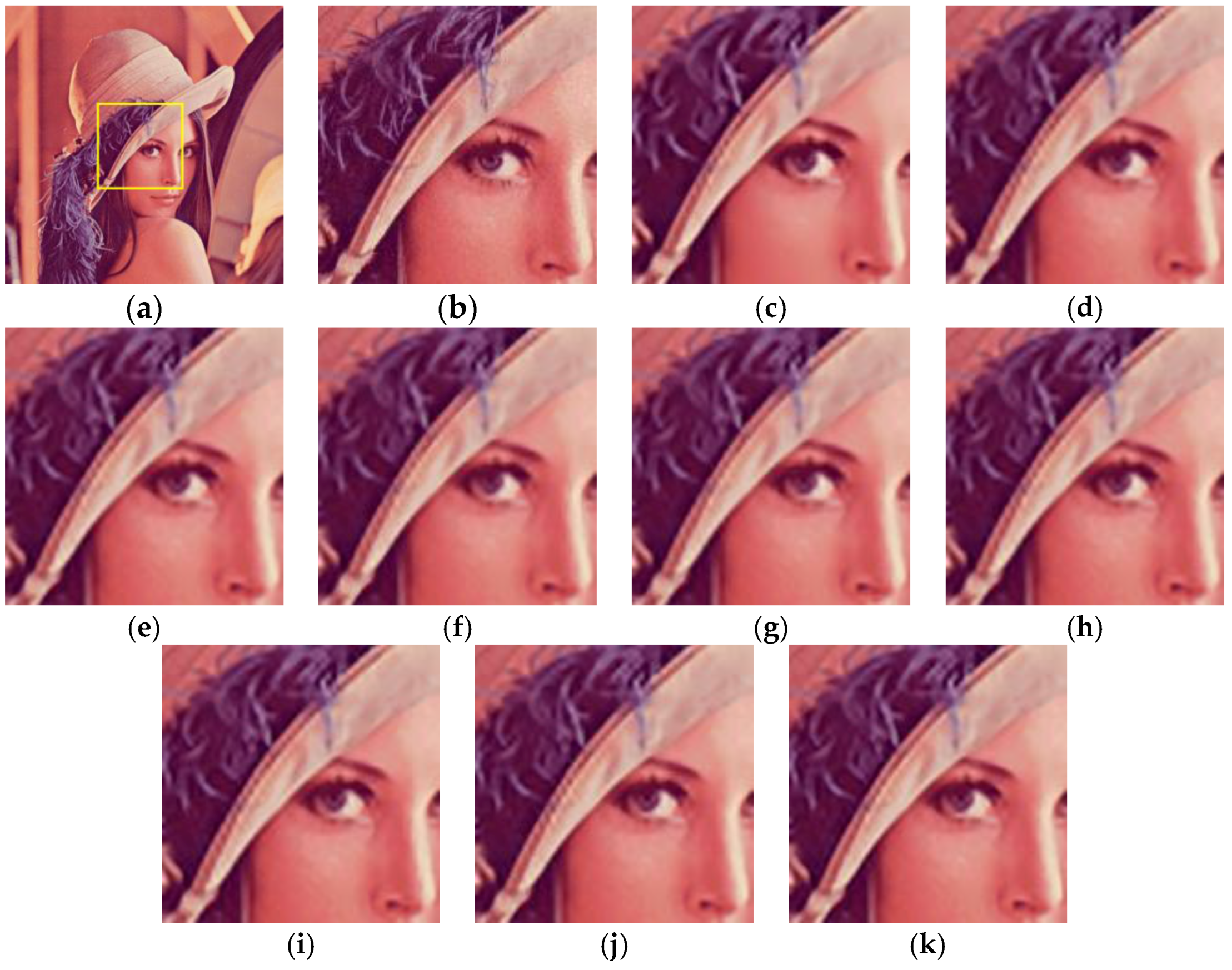
Figure 7a,b and Figure 8a,b show the two HR test images Lena and Bird and their corresponding detail images, respectively. Figure 7c–k and Figure 8c–k, respectively, illustrate the reconstructed results of the detail regions of the brim of Lena’s hat and the Bird’s head with different SR algorithms from subjective visual perception. It can be seen from Figure 7 and Figure 8 that although the L1SR algorithm restores some parts of the details, there are obvious patch effects in its reconstructed images, such as the face in Figure 7c and part of the yellow feather in Figure 8c. With the SISR algorithm, the edge sharpening effect is obvious, but some artificial details appear in the reconstructed images, such as the edge of the hat in Figure 7d. The SR algorithms corresponding to Figure 7e–j and Figure 8e–j achieve good reconstructed results, but too many artificial details, such as the brim of Lena’s hat and the junction of the bottom of the Bird’s mouth and feather in those reconstructed results, are introduced while restoring more details. The proposed SRISAE algorithm is superior to the other eight SR algorithms. It restores more details without introducing too many artificial details, and the areas of the brim of Lena’s hat in Figure 7k and the junction of the bottom of the Bird’s mouth and feather in Figure 8k are closer to the original images. Table 3 shows the PSNR and SSIM values of the reconstructed images with different SR algorithms for these test images. It can be seen from Table 3 that the PSNR and SSIM values of the SRISAE algorithm are generally optimal, which indicates that the proposed SRISAE algorithm outperforms the other eight SR algorithms mentioned above.
To analyze the computing time of these SR algorithms, our experiments are performed on the same hardware platform mentioned above, and the computing time of different SR algorithms is shown in Table 4. From Table 4, we can see that although the time the proposed SRISAE algorithm spent is not the least, it is at the same level as the algorithms including SISR, ANR, NE + LS, NE + NNLS, NE + LLE, and A + (16 atoms), and its reconstruction performance is superior to these algorithms. It can be seen from Table 3 and Table 4 that SRISAE significantly outperforms ISPSR in terms of computing time despite its small increase relative to ISPSR in terms of the PSNR and SSIM indices. Through a comprehensive analysis, we can see that the proposed SRISAE algorithm not only has the best reconstruction performance, but also has good reconstruction efficiency.
Table 5 lists the average PSNR and SSIM values of the reconstructed images with different SR algorithms mentioned above for B100. It can be seen from Table 5 that the average of these two evaluation indices of the proposed algorithm are optimal, indicating that the performance of our algorithm is better than that of the comparative SR algorithms.
5.2.4. Analyze the Performance of Different SR Algorithms on Real Medical Images
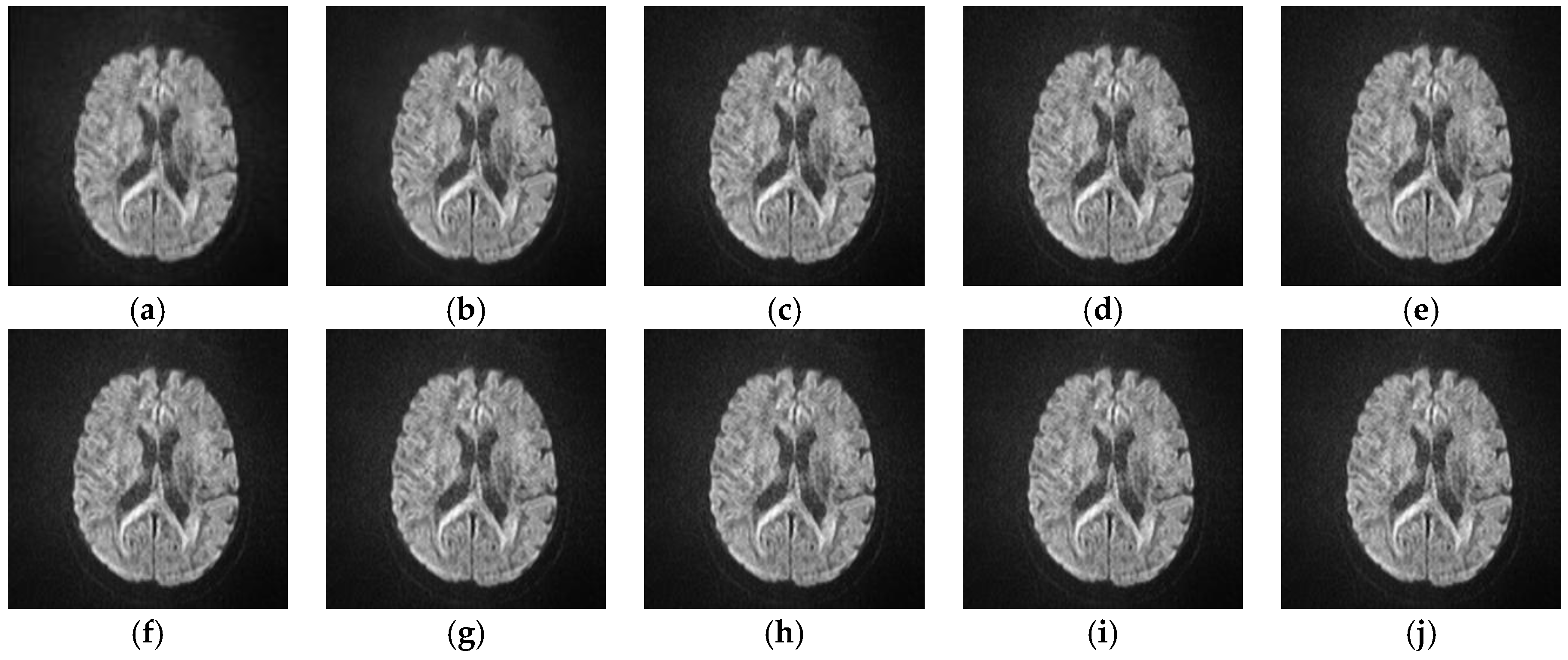
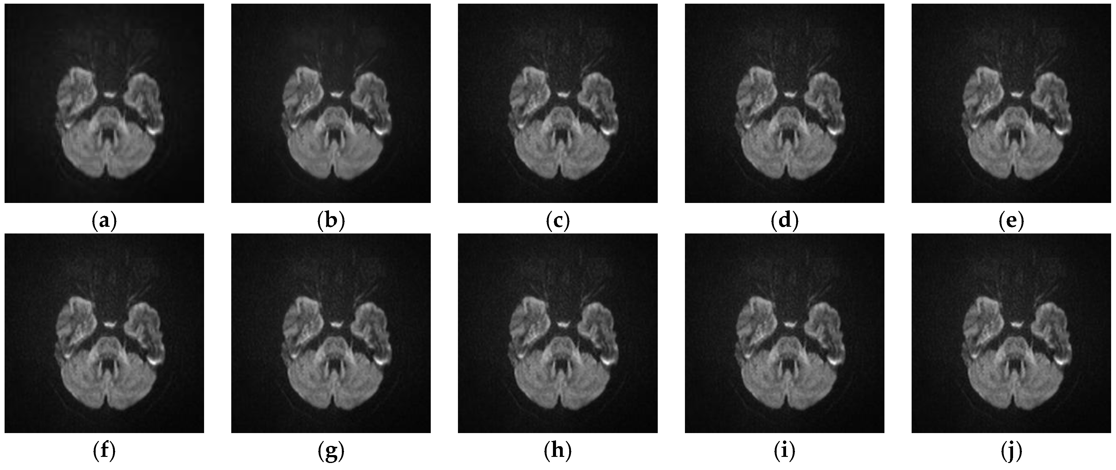
This experiment is to test the performance of different SR algorithms on bad quality medical images. The training data and the test data are derived from the published data set The Cancer Imaging Archive (TCIA) [36] and the test images are real LR medical images which have been randomly selected. Figure 9 and Figure 10 illustrate the reconstructed images of two real lung cancer images with different SR algorithms. Among them, Figure 9j and Figure 10j are the reconstructed images of the proposed SRISAE algorithm. Comparing them with the real LR images to be reconstructed shown in Figure 9a and Figure 10a, the reconstructed images of the SRISAE algorithm are clearer and many details in the edge, texture, and structure are restored.
Since there is no HR reference image, some classic no-reference image quality evaluation indices are used to evaluate the reconstructed images of different SR algorithms objectively. The indices are Variance, Meangradient, Entropy, Brenner, and Energy [37,38], and the higher the value is, the better the reconstructed performance. The maximum values of these indices are highlighted in bold type. Table 6 shows the average of these indices of 76 reconstructed medical images, and we can see that the proposed SRISAE algorithm is slightly better than the other eight SR algorithms. (a) input; (b) L1SR; (c) SISR; (d) ANR; (e) NE + LS; (f) NE + NNLS; (g) NE + LLE; (h) A + (16 atoms); (i) ISPSR; (j) SRISAE.
6. Conclusions
To make the input data more effective and enhance the training efficiency of the SAE, we propose a new training set preprocessing method which utilizes different approaches to construct HR and LR training sets and employs the ZCA whitening technology to decorrelate the joint training set to reduce its redundancy. The SAE is applied to the SR algorithm based on sparse representation, and to further enhance the sparsity of the hidden layer, a constructed sparse regularization term is added to the cost function of the traditional SAE. Then, a novel unsupervised dictionary learning algorithm based on the ISAE is proposed to improve the accuracy and stability of the dictionary. Comparisons with several SR algorithms, including L1SR, SISR, ANR, NE + LS, NE + NNLS, NE + LLE, A + (16 atoms) and ISPSR are made. Experimental results demonstrate that the proposed SRISAE algorithm achieves a significant improvement in terms of both quantitative and qualitative measurements.
Acknowledgments
The authors would like to thank all of the reviewers for their constructive comments. This work is supported by the Nature Science Foundation of China (Grant No. 61672335, No. 61602191) and by the Foundation of Fujian Education Department under Grant No. JAT170053.
Author Contributions
Detian Huang and Weiqin Huang conceived and designed the experiments; Weiqin Huang and Zhenguo Yuan performed the experiments; Yanming Lin and Jian Zhang analyzed the data; Lixin Zheng contributed reagents/materials/analysis tools; Detian Huang and Weiqin Huang wrote the paper.
Conflicts of Interest
The authors declare no conflict of interest.
References
- Pan, Z.X.; Yu, J.U.; Xiao, C.B.; Sun, W.D. Single image super resolution based on adaptive multi-dictionary learning. Acta Electron. Sin. 2015, 43, 209–216. [Google Scholar]
- Huang, D.T.; Huang, W.Q.; Huang, H.; Zheng, L.X. Application of regularization technique in image super-resolution algorithm via sparse representation. Optoelectron. Lett. 2017, 13, 439–443. [Google Scholar] [CrossRef]
- Olshausen, B.A.; Field, D.J. Sparse coding with an overcomplete basis set: A strategy employed by V1? Vis. Res. 1997, 37, 3311–3325. [Google Scholar] [CrossRef]
- Lee, D.D.; Seung, H.S. Learning the parts of objects by non-negative matrix factorization. Nature 1999, 401, 788–791. [Google Scholar] [PubMed]
- Elad, M.; Aharon, M. Image denoisingvia sparse and redundant representations over learned dictionaries. IEEE Trans. Image Process. 2006, 15, 3736–3745. [Google Scholar] [CrossRef] [PubMed]
- Koh, M.S.; Rodriguez-Marek, E. Turbo inpainting: Iterative K-SVD with a new dictionary. In Proceedings of the IEEE International Workshop on Multimedia Signal Processing, Rio De Janeiro, Brazil, 5–7 October 2009; pp. 1–6. [Google Scholar]
- Mairal, J.; Elad, M.; Sapiro, G. Sparse representation for color image restoration. IEEE Trans. Image Process. 2008, 17, 53–69. [Google Scholar] [CrossRef] [PubMed]
- Son, C.H.; Choo, H. Local learned dictionaries optimized to edge orientation for inverse halftoning. IEEE Trans. Image Process. 2014, 23, 2542–2556. [Google Scholar] [PubMed]
- Caballero, J.; Price, A.N.; Rueckert, D.; Hajnal, J.V. Dictionary learning and time sparsity for dynamic MR data reconstruction. IEEE Trans. Med. Imaging 2014, 33, 979–994. [Google Scholar] [CrossRef] [PubMed]
- Majumdar, A.; Ward, R. Learning space-time dictionaries for blind compressed sensing dynamic MRI reconstruction. In Proceedings of the IEEE International Conference on Image Processing (ICIP), Quebec City, QC, Canada, 27–30 September 2015; pp. 4550–4554. [Google Scholar]
- Jadhav, D.V.; Holambe, R.S. Feature extraction using Radon and wavelet transforms with application to face recognition. Neurocomputing 2009, 72, 1951–1959. [Google Scholar] [CrossRef]
- Dabbaghchian, S.; Ghaemmaghami, M.P.; Aghagolzadeh, A. Feature extraction using discrete cosine transform and discrimination power analysis with a face recognition technology. Pattern Recognit. 2010, 43, 1431–1440. [Google Scholar] [CrossRef]
- Engan, K.; Aase, S.O.; Husoy, J.H. Frame based signal compression using method of optimal directions (MOD). In Proceedings of the IEEE International Symposium on Circuits and Systems, Orlando, FL, USA, 30 May–2 June 1999; Volume 4, pp. 1–4. [Google Scholar]
- Aharon, M.; Elad, M.; Bruckstein, A. rm K-SVD: An algorithm for designing overcomplete dictionaries for sparse representation. IEEE Trans. Signal Process. 2006, 54, 4311–4322. [Google Scholar] [CrossRef]
- Mairal, J.; Bach, F.; Ponce, J.; Sapiro, G. Online learning for matrix factorization and sparse coding. J. Mach. Learn. Res. 2010, 11, 19–60. [Google Scholar]
- Singhal, V.; Gogna, A.; Majumdar, A. Deep dictionary learning vs deep belief network vs stacked autoencoder: An empirical analysis. In Proceedings of the International Conference on Neural Information Processing, Kyoto, Japan, 16–21 October 2016; Springer: Cham, Switzerland, 2016; pp. 337–344. [Google Scholar]
- Yang, J.; Wright, J.; Huang, T.S.; Ma, Y. Image super-resolution via sparse representation. IEEE Trans. Image Process. 2010, 19, 2861–2873. [Google Scholar] [CrossRef] [PubMed]
- Zeyde, R.; Elad, M.; Protter, M. On single image scale-up using sparse-representations. In Proceedings of the International Conference on Curves and Surfaces, Avignon, France, 24–30 June 2010; Volume 6920, pp. 711–730. [Google Scholar]
- Jing, X.Y.; Zhu, X.; Wu, F.; Hu, R.; You, X.; Wang, Y.; Feng, H.; Yang, J.Y. Super-resolution person re-identification with semi-coupled low-rank discriminant dictionary learning. IEEE Trans. Image Process. 2015, 26, 1363–1378. [Google Scholar] [CrossRef] [PubMed]
- Zhang, X.; Zhou, W.; Duan, Z. Image super-resolution reconstruction based on fusion of K-SVD and semi-coupled dictionary learning. In Proceedings of the Asia-Pacific Signal and Information Processing Association Annual Summit and Conference (APSIPA), Jeju, Korea, 13–16 December 2016; pp. 1–5. [Google Scholar]
- Zhang, Y.; Liu, Y. Single image super-resolution reconstruction method based on LC-KSVD algorithm. AIP Conf. Proc. 2017, 1521–1527. [Google Scholar] [CrossRef]
- Zhang, H.; Liu, X.; Yang, S.; Yu, L.I. Retrieval of remote sensing images based on semisupervised deep learning. J. Remote Sens. 2017, 21, 406–414. [Google Scholar]
- Donoho, D.L. For most large underdetermined systems of equations, the minimal ℓ1-norm near-solution approximates the sparsest near-solution. Commun. Pure Appl. Math. 2010, 59, 797–829. [Google Scholar] [CrossRef]
- Merola, G.M. SPCA: Sparse principal component analysis. Pattern Recognit. Lett. 2014, 34, 1037–1045. [Google Scholar]
- Krizhevsky, A. Learning Multiple Layers of Features from Tiny Images; Technical Report; University of Toronto: Toronto, ON, Canada, 2009. [Google Scholar]
- Ng, A. Sparse Autoencoder; CS294A Lecture Notes; Stanford University: Stanford, CA, USA, 2011; Volume 72, pp. 1–19. [Google Scholar]
- Miller, F.P.; Vandome, A.F.; Mcbrewster, J. Gradient Descent; Alphascript Publishing: Saarbrücken, Germany, 2010; Volume 20, pp. 235–242. [Google Scholar]
- Li, X.F.; Zeng, L.; Xu, J.; Ma, S.Q. Single image super-resolution based on the feature sign method. J. Univ. Electron. Sci. Technol. China 2015, 44, 22–27. [Google Scholar]
- Huang, D.T.; Huang, W.Q.; Gu, P.T.; Liu, P.Z.; Luo, Y.M. Image super-resolution reconstruction based on regularization technique and guided filter. Infrared Phys. Technol. 2017, 83, 103–113. [Google Scholar] [CrossRef]
- Wang, Y.; Li, J.; Lu, Y.; Fu, Y. Image quality evaluation based on image weighted separating block peak signal to noise ratio. In Proceedings of the IEEE International Conference on Neural Networks and Signal Processing, Nanjing, China, 14–17 December 2003; Volume 2, pp. 994–997. [Google Scholar]
- Wang, Z.; Bovik, A.C.; Sheikh, H.R.; Simoncelli, E.P. Image quality assessment: From error visibility to structural similarity. IEEE Trans. Image Process. 2004, 13, 600–612. [Google Scholar] [CrossRef] [PubMed]
- Bevilacqua, M.; Roumy, A.; Guillemot, C.; Morel, A. Low-complexity single-image super-resolution based on nonnegative neighbor embedding. In Proceedings of the British Machine Vision Conference, Guildford, UK, 3–7 September 2012; pp. 1–10. [Google Scholar]
- Martin, D.; Fowlkes, C.; Tal, D.; Malik, J. A database of human segmented natural images and its application to evaluating segmentation algorithms and measuring ecological statistics. In Proceedings of the IEEE International Conference on Computer Vision, Vancouver, BC, Canada, 7–14 July 2001; pp. 416–423. [Google Scholar]
- Timofte, R.; De, V.; Gool, L.V. Anchored neighborhood regression for fast example-based super-resolution. In Proceedings of the IEEE International Conference on Computer Vision (ICCV), Sydney, Australia, 1–8 December 2013; pp. 1920–1927. [Google Scholar]
- Timofte, R.; Smet, V.D.; Gool, L.V. A+: Adjusted Anchored Neighborhood Regression for Fast Super-Resolution. Asian Conference on Computer Vision; Springer: Cham, Switzerland, 2014; Volume 9006, pp. 111–126. [Google Scholar]
- Clark, K.; Vendt, B.; Smith, K.; Freymann, J.; Koppel, P.; Moore, S.; Phillips, S.; Maffitt, D.; Pringle, M.; Tarbox, L.; et al. The Cancer Imaging Archive (TCIA): Maintaining and operating a public information repository. J. Digit. Imaging 2013, 26, 1045–1057. [Google Scholar] [CrossRef] [PubMed]
- Wang, H.N.; Zhong, W.; Wang, J.; Xia, D.S. Research of measurement for Digital Image Definition. J. Image Graph. 2004, 9, 828–831. [Google Scholar]
- Li, Z.L.; Li, X.H.; Ma, L.L.; Hu, Y.; Tang, L.L. Research of Definition Assessment based on No-reference Digital Image Quality. Remote Sens. Technol. Appl. 2011, 26, 239–246. [Google Scholar]
Figure 1.
Framework of the proposed training set preprocessing method. HR: high resolution; LR: low resolution; ZCA: zero-phase component analysis.
Figure 1.
Framework of the proposed training set preprocessing method. HR: high resolution; LR: low resolution; ZCA: zero-phase component analysis.

Figure 2.
Relationship between dictionary learning and neural network representation. (a) Dictionary learning; (b) Neural network representation.
Figure 2.
Relationship between dictionary learning and neural network representation. (a) Dictionary learning; (b) Neural network representation.

Figure 3.
Sparse autoencoder (SAE) structure.

Figure 4.
Some training samples for dictionary learning.

Figure 5.
Reconstructed results of Butterfly using the dictionaries with different numbers of hidden units. (a) Butterfly; (b) Reference; (c) Bicubic; (d) Hidden units 256; (e) Hidden units 512; (f) Hidden units 1024; (g) Hidden units 2048.
Figure 5.
Reconstructed results of Butterfly using the dictionaries with different numbers of hidden units. (a) Butterfly; (b) Reference; (c) Bicubic; (d) Hidden units 256; (e) Hidden units 512; (f) Hidden units 1024; (g) Hidden units 2048.

Figure 6.
Comparison of the reconstructed images with three SR algorithms for Woman. (a) Woman; (b) Reference; (c) Bicubic; (d) SRSAE; (e) SRISAE.
Figure 6.
Comparison of the reconstructed images with three SR algorithms for Woman. (a) Woman; (b) Reference; (c) Bicubic; (d) SRSAE; (e) SRISAE.

Figure 7.
Comparison of the reconstructed images with different SR algorithms for Lena. L1SR: Super Resolution with L1 Regression; SISR: Single Image Super Resolution; ANR: Anchored Neighborhood Regression; NE + LS: Neighbor Embedding with Least Squares; NE + NNLS: Neighbor Embedding with Non-Negative Least Square; NE + LLE: Neighbor Embedding with Locally Linear Embedding; A + (16 atoms): Adjusted Anchored Neighborhood Regression; ISPSR: improved Super Resolution based on Sparse representation; SRISAE: SR algorithm based on the ISAE. (a) Lena; (b) Reference; (c) L1SR; (d) SISR; (e) ANR; (f) NE + LS; (g) NE + NNLS; (h) NE + LLE; (i) A + (16 atoms); (j) ISPSR; (k) SRISAE.

Figure 8.
Comparison of the reconstructed images with different SR algorithms for Bird. (a) Bird; (b) Reference; (c) L1SR; (d) SISR; (e) ANR; (f) NE + LS; (g) NE + NNLS; (h) NE + LLE; (i) A + (16 atoms); (j) ISPSR; (k) SRISAE.
Figure 8.
Comparison of the reconstructed images with different SR algorithms for Bird. (a) Bird; (b) Reference; (c) L1SR; (d) SISR; (e) ANR; (f) NE + LS; (g) NE + NNLS; (h) NE + LLE; (i) A + (16 atoms); (j) ISPSR; (k) SRISAE.

Figure 9.
Comparison of the reconstructed images with different SR algorithms for medical image1. (a) input; (b) L1SR; (c) SISR; (d) ANR; (e) NE + LS; (f) NE + NNLS; (g) NE + LLE; (h) A + (16 atoms); (i) ISPSR; (j) SRISAE.
Figure 9.
Comparison of the reconstructed images with different SR algorithms for medical image1. (a) input; (b) L1SR; (c) SISR; (d) ANR; (e) NE + LS; (f) NE + NNLS; (g) NE + LLE; (h) A + (16 atoms); (i) ISPSR; (j) SRISAE.

Figure 10.
Comparison of the reconstructed images with different SR algorithms for medical image2.


Table 1.
Comparison of the peak signal-to-noise ratio PSNR (dB) and the structural similarity measure (SSIM) of the reconstructed images using the dictionaries with different numbers of hidden units for Set5 (PSNR/SSIM).
Table 1.
Comparison of the peak signal-to-noise ratio PSNR (dB) and the structural similarity measure (SSIM) of the reconstructed images using the dictionaries with different numbers of hidden units for Set5 (PSNR/SSIM).
| Images | 256 | 512 | 1024 | 2048 |
|---|---|---|---|---|
| Baby | 35.20/0.9425 | 35.06/0.9411 | 35.23/0.9426 | 35.26/0.9428 |
| Bird | 34.52/0.9616 | 34.68/0.9618 | 35.36/0.9666 | 35.14/0.9658 |
| Butterfly | 25.71/0.8947 | 26.39/0.9077 | 26.63/0.9179 | 26.48/0.9174 |
| Head | 33.61/0.8604 | 33.62/0.8606 | 33.82/0.8624 | 33.71/0.8621 |
| Woman | 30.15/0.9344 | 30.49/0.9370 | 30.81/0.9421 | 30.73/0.9417 |
| Average | 31.84/0.9187 | 32.05/0.9216 | 32.37/0.9263 | 32.26/0.9260 |
Table 2.
Comparison of the average PSNR(dB) and SSIM values of the reconstructed images with the three super resolution (SR) algorithms for Set5, Set14, and BSD100 (PSNR/SSIM). SRSAE: SR algorithm based on the SAE; SRISAE: SR algorithm based on the ISAE.
Table 2.
Comparison of the average PSNR(dB) and SSIM values of the reconstructed images with the three super resolution (SR) algorithms for Set5, Set14, and BSD100 (PSNR/SSIM). SRSAE: SR algorithm based on the SAE; SRISAE: SR algorithm based on the ISAE.
| Images | Bicubic | SRSAE | SRISAE |
|---|---|---|---|
| Set5 | 30.40/0.8953 | 32.16/0.9234 | 32.37/0.9263 |
| Set4 | 27.54/0.8107 | 28.90/0.8487 | 28.99/0.8503 |
| BSD100 | 27.15/0.7775 | 28.03/0.8169 | 28.19/0.8180 |
Table 3.
Comparison of the PSNR and the SSIM of the reconstructed images with different SR algorithms (PSNR/SSIM).
Table 3.
Comparison of the PSNR and the SSIM of the reconstructed images with different SR algorithms (PSNR/SSIM).
| Images | PSNR/SSIM | L1SR | SISR | ANR | NE + LS | NE + NNLS | NE + LLE | A + (16 Atoms) | ISPSR | SRISAE |
|---|---|---|---|---|---|---|---|---|---|---|
| baby | PSNR | 34.29 | 35.08 | 35.13 | 34.96 | 34.77 | 35.06 | 35.13 | 35.23 | 35.23 |
| SSIM | 0.9226 | 0.9402 | 0.9415 | 0.9390 | 0.9370 | 0.9401 | 0.9409 | 0.9426 | 0.9426 | |
| bird | PSNR | 34.11 | 34.57 | 34.60 | 34.36 | 34.26 | 34.56 | 34.83 | 35.25 | 35.36 |
| SSIM | 0.9530 | 0.9615 | 0.9623 | 0.9602 | 0.9581 | 0.9615 | 0.9629 | 0.9663 | 0.9666 | |
| Head | PSNR | 33.17 | 33.56 | 33.63 | 33.53 | 33.45 | 33.60 | 33.65 | 33.74 | 33.82 |
| SSIM | 0.8382 | 0.8572 | 0.8600 | 0.8569 | 0.8554 | 0.8590 | 0.8606 | 0.8616 | 0.8624 | |
| flowers | PSNR | 28.25 | 28.43 | 28.49 | 28.35 | 28.21 | 28.38 | 28.52 | 28.74 | 28.85 |
| SSIM | 0.8636 | 0.8713 | 0.8739 | 0.8697 | 0.8673 | 0.8718 | 0.8745 | 0.8801 | 0.8818 | |
| Lena | PSNR | 32.64 | 33.00 | 33.08 | 32.98 | 32.82 | 33.01 | 33.17 | 33.37 | 33.53 |
| SSIM | 0.8852 | 0.9002 | 0.9022 | 0.9000 | 0.8981 | 0.9010 | 0.9027 | 0.9050 | 0.9055 | |
| monarch | PSNR | 30.71 | 31.10 | 31.09 | 30.94 | 30.76 | 30.95 | 31.31 | 31.74 | 31.95 |
| SSIM | 0.9422 | 0.9510 | 0.9508 | 0.9499 | 0.9478 | 0.9495 | 0.9518 | 0.9558 | 0.9559 | |
| pepper | PSNR | 33.33 | 34.07 | 33.82 | 33.91 | 33.56 | 33.80 | 34.01 | 34.28 | 34.55 |
| SSIM | 0.8851 | 0.9060 | 0.9045 | 0.9046 | 0.9017 | 0.9041 | 0.9052 | 0.9080 | 0.9098 | |
| ppt3 | PSNR | 24.98 | 25.23 | 25.03 | 25.15 | 24.81 | 24.94 | 25.22 | 25.62 | 25.89 |
| SSIM | 0.9025 | 0.9204 | 0.9123 | 0.9193 | 0.9077 | 0.9111 | 0.9147 | 0.9298 | 0.9291 | |
| Average | PSNR | 31.44 | 31.88 | 31.86 | 31.77 | 31.58 | 31.79 | 31.98 | 32.25 | 32.40 |
| SSIM | 0.8991 | 0.9299 | 0.9098 | 0.9297 | 0.9011 | 0.9054 | 0.9116 | 0.9187 | 0.9195 |
Table 4.
Comparison of computing time of different SR algorithms (s).
| Image | L1SR | SISR | ANR | NE + LS | NE + NNLS | NE + LLE | A + (16 Atoms) | ISPSR | SRISAE |
|---|---|---|---|---|---|---|---|---|---|
| baby | 194.41 | 1.92 | 0.52 | 1.72 | 9.83 | 2.26 | 0.43 | 1309.44 | 3.28 |
| bird | 63.15 | 0.60 | 0.18 | 0.54 | 3.04 | 0.72 | 0.14 | 408.16 | 1.05 |
| Head | 55.42 | 0.55 | 0.16 | 0.50 | 2.87 | 0.64 | 0.13 | 378.57 | 1.02 |
| flowers | 141.14 | 1.40 | 0.37 | 1.19 | 6.78 | 1.60 | 0.30 | 899.02 | 2.24 |
| Lena | 187.96 | 1.91 | 0.51 | 1.72 | 9.70 | 2.27 | 0.43 | 1296.17 | 3.29 |
| monarch | 81.33 | 2.91 | 0.78 | 2.608 | 15.05 | 3.43 | 0.65 | 1974.27 | 5.06 |
| pepper | 186.37 | 1.92 | 0.53 | 1.73 | 9.87 | 2.25 | 0.44 | 1294.75 | 3.26 |
| ppt3 | 222.23 | 2.30 | 0.68 | 2.17 | 11.91 | 2.94 | 0.57 | 1727.80 | 4.08 |
| Average | 141.50 | 1.69 | 0.47 | 1.52 | 8.63 | 2.01 | 0.39 | 1161.02 | 2.91 |
Table 5.
Comparison of the average of PSNR and SSIM of the reconstructed images with different SR algorithms for B100 (PSNR/SSIM).
Table 5.
Comparison of the average of PSNR and SSIM of the reconstructed images with different SR algorithms for B100 (PSNR/SSIM).
| B100 | PSNR/SSIM | L1SR | SISR | ANR | NE + LS | NE + NNLS | NE + LLE | A + (16 Atoms) | ISPSR | SRISAE |
|---|---|---|---|---|---|---|---|---|---|---|
| Average | PSNR | 27.72 | 27.87 | 27.89 | 27.83 | 27.73 | 27.85 | 27.94 | 28.07 | 28.19 |
| SSIM | 0.800 | 0.809 | 0.812 | 0.809 | 0.806 | 0.811 | 0.814 | 0.8176 | 0.8180 |
Table 6.
Comparison of the average of no-reference image quality evaluation indices of the reconstructed images with different SR algorithms.
Table 6.
Comparison of the average of no-reference image quality evaluation indices of the reconstructed images with different SR algorithms.
| Indices | L1SR | SISR | ANR | NE + LS | NE + NNLS | NE + LLE | A + (16 Atoms) | ISPSR | SRISAE |
|---|---|---|---|---|---|---|---|---|---|
| Variance | 2446.8651 | 2479.3577 | 2483.4034 | 2480.6194 | 2478.4239 | 2481.2642 | 2483.7900 | 2483.0294 | 2486.2215 |
| Meangradient | 2.8012 | 3.2414 | 3.4120 | 3.2862 | 3.2877 | 3.4117 | 3.4927 | 3.4435 | 3.5033 |
| Entropy | 6.4871 | 6.5141 | 6.5256 | 6.5180 | 6.5170 | 6.5268 | 6.5275 | 6.5231 | 6.5383 |
| Brenner | 4,596,865 | 5,243,693 | 5,568,487 | 5,273,747 | 5,292,623 | 5,457,148 | 5,776,475 | 5,863,142 | 5,914,784 |
| Energy | 4,167,251 | 4,369,326 | 4,644,846 | 4,526,663 | 4,532,565 | 4,544,087 | 4,981,985 | 4,986,970 | 5,098,674 |
© 2018 by the authors. Licensee MDPI, Basel, Switzerland. This article is an open access article distributed under the terms and conditions of the Creative Commons Attribution (CC BY) license (http://creativecommons.org/licenses/by/4.0/).
Share and Cite
MDPI and ACS Style
Huang, D.; Huang, W.; Yuan, Z.; Lin, Y.; Zhang, J.; Zheng, L. Image Super-Resolution Algorithm Based on an Improved Sparse Autoencoder. Information 2018, 9, 11. https://doi.org/10.3390/info9010011
AMA Style
Huang D, Huang W, Yuan Z, Lin Y, Zhang J, Zheng L. Image Super-Resolution Algorithm Based on an Improved Sparse Autoencoder. Information. 2018; 9(1):11. https://doi.org/10.3390/info9010011
Chicago/Turabian StyleHuang, Detian, Weiqin Huang, Zhenguo Yuan, Yanming Lin, Jian Zhang, and Lixin Zheng. 2018. "Image Super-Resolution Algorithm Based on an Improved Sparse Autoencoder" Information 9, no. 1: 11. https://doi.org/10.3390/info9010011
Note that from the first issue of 2016, this journal uses article numbers instead of page numbers. See further details here.