An Improved Progressive TIN Densification Filtering Method Considering the Density and Standard Variance of Point Clouds

Abstract

The progressive TIN (triangular irregular network) densification (PTD) filter algorithm is widely used for filtering point clouds. In the PTD algorithm, the iterative densification parameters become smaller over the entire process of filtering. This leads to the performance—especially the type I errors of the PTD algorithm—being poor for point clouds with high density and standard variance. Hence, an improved PTD filtering algorithm for point clouds with high density and variance is proposed in this paper. This improved PTD method divides the iterative densification process into two stages. In the first stage, the iterative densification process of the PTD algorithm is used, and the two densification parameters become smaller. When the density of points belonging to the TIN is higher than a certain value (in this paper, we define this density as the standard variance intervention density), the iterative densification process moves into the second stage. In the second stage, a new iterative densification strategy based on multi-scales is proposed, and the angle threshold becomes larger. The experimental results show that the improved PTD algorithm can effectively reduce the type I errors and total errors of the DIM point clouds by 7.53% and 4.09%, respectively, compared with the PTD algorithm. Although the type II errors increase slightly in our improved method, the wrongly added objective points have little effect on the accuracy of the generated DSM. In short, our improved PTD method perfects the classical PTD method and offers a better solution for filtering point clouds with high density and standard variance.

1. Introduction

Point clouds (including light detection and ranging (LiDAR) point clouds and dense image matching (DIM) point clouds have been widely used in various fields, such as land cover classification [1], canopy detection and vegetation analysis [2,3], the reconstruction of digital terrain models (DTM) [4], etc. In these applications, point clouds filtering is an essential step. Over the past two decades, various filtering algorithms have been proposed for the separation of ground points and off-ground points. According to the filter concept proposed in Ref. [5], these filtering algorithms can be divided into four categories: surface-based filtering [6,7,8], slope-based filtering [9,10,11], clustering and segmentation [12,13,14,15] and minimum-block-based filtering [16,17,18]. An experimental comparison of eight commonly used filtering algorithms was conducted by Sithole and Vosselman [5]. The experimental results in the paper show that surface-based filtering algorithms perform better than other filtering algorithms.

According to the previous study, the surface-based filtering algorithms are divided into three sub-categories: morphology-based filtering [19,20,21,22], iterative-interpolation-based filtering [23,24] and progressive-densification-based filters [25,26,27,28]. Among the surface-based filtering algorithms, the progressive TIN (triangular irregular network) densification (PTD) algorithm proposed by Axelsson [25] is most widely used because of its robustness and effectiveness in the separation of ground points and non-ground points. Even though the PTD algorithm can perform well for both airborne LiDAR system (ALS) point clouds and DIM point clouds, this method still has some limitations. Aiming at these limitations, some improved PTD algorithms are proposed.

Lin et al. [26] used a segment instead of a single point as a basic processing unit to filter the point clouds. The experimental results show this method can remove the lower parts of large objects attached on the ground surface. Wang et al. [27] revised the iterative densification process of the PTD algorithm. Specifically, they first divided the ground points into grids; then, selected a lowest point as the ground point and classified other points as non-ground points to be judged by the thresholds again within each grid; and densified the TIN until the ratio of the difference calculated by the last two new ground points added into the TIN to the total points is less than a given threshold during two consecutive iterations. Compared with the classic PTD method, this algorithm can obtain smooth bare-earth and remove the low objective points. Nie et al. [28] applied a method similar to the Douglas–Peuker algorithm to build an improved TIN. In the stage of iterative densification, only one point, the distance of which to the corresponding TIN facet is minimum among all potential ground points, is selected as the ground point. Moreover, to preserve the ground measurements, the angle threshold is greater than the given maximum threshold in the stage of parameter specification. The biggest advantage of this method is to remove point clouds belonging to lower objects and preserve ground measurements in topographically complex areas.

From the analysis of these improved methods, we can see that these improved methods mainly focus on removing point clouds belonging to lower objects. However, in some applications, such as object classifications [29], lowering the type I errors also plays an important role so that the ground points can be extracted from point clouds completely. Moreover, the PTD algorithm does not consider the influence of the density and standard variance of point clouds on the filtering performance. In fact, when the PTD algorithm is applied for the point clouds with high density and standard variance, the type I errors can reach 40% [30]. Furthermore, experimental results [30,31] show that the higher the density and standard variance of point clouds are, the worse the performance of the PTD algorithm is.

To remove the ground points from point clouds with high density completely, researchers [1,32,33,34] rarefied the point clouds with high density and standard variance at first; then used the PTD algorithm to obtain the ground points and construct the digital terrain model (DTM); and, finally, calculated the distance from an unclassified point to the DTM. If this distance is lower than a given threshold, this point is regarded as a ground point; otherwise, it is a non-ground point. However, this method has two limitations:

• The rarefied points may miss the topographic features and the constructed DTM cannot reflect the true ground surface.
• The threshold is difficult to determine. If the given threshold is higher than the real threshold, objective points will be regarded as ground points. If the given threshold is lower than the real threshold, the ground points cannot be removed completely.

Therefore, this paper analyzes how the density and standard variance of point clouds impact the filtering performance of the PTD method. Based on the analysis, an improved PTD algorithm is proposed. The main difference between the classical PTD algorithm and the improved PTD algorithm is the change of densification parameters in the process of iterative densification. In the entire iterative densification process of the classical PTD method, the angle threshold and distance threshold become smaller, whereas, in the improved PTD algorithm, the angle threshold of our improved method becomes smaller in the first stage and then becomes larger in the second stage. Notably, the change of the angle threshold in our proposed method is different from the change of angle threshold in Ref. [28]. In Ref. [28], the angle threshold is only greater than the maximum angle value which is specified at the stage of the parameter input. It is a fixed value. In our proposed method, the angle threshold is changing during the process of iterative densification. Based on the angle threshold, the process of densification of the improved PTD algorithm is divided into two stages:

• In the first stage, the densification strategy of the classical PTD algorithm is used; and the initial TIN is densified until the density of points belonging to the TIN reaches a certain value (in this paper, we define the value as the standard variance intervention density).
• In the second stage, a new strategy based on multi-scales for densification is proposed. In this densification strategy, a contour interpolation method based-triangulation is used for the calculation of densification parameters.

To evaluate the performance of our proposed method, the Vaihingen dataset, which contains the ALS data and aerial images, was selected. With the aid of the commercial software package PhotoScan [35], the aerial images were converted into the DIM point clouds which have the high density and standard variance. The experimental results show that our proposed method can reduce the type I errors efficiently and constrain the increase of type II errors. The rest of this paper is organized as follows:

• Section 2 analyzes how the density and standard variance of point clouds impact the performance of the classical PTD algorithm and details the improved PTD algorithm.
• Section 3 presents the performance evaluation and discusses the experimental results using two test patches of the Vaihingen dataset followed by a comparative analysis.
• Section 4 concludes the paper.

2. Methodology

2.1. PTD Algorithm

The classical PTD algorithm is an iterative process, wherein an initial TIN consisting of seed points is densified. The process can be divided into three steps:

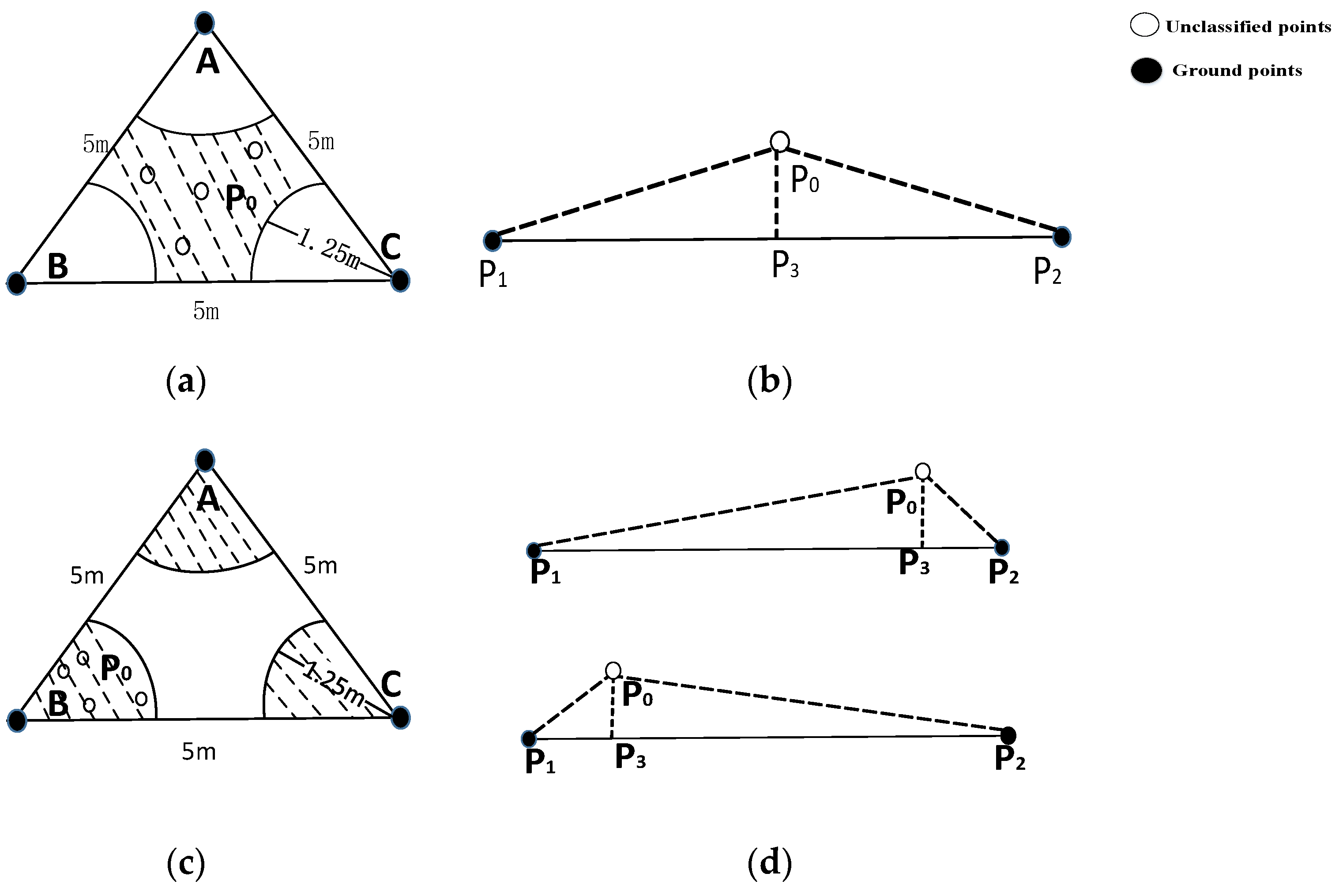
• Parameter input. According to the commercial software TerraSolid, five key parameters should be determined in the PTD algorithm: $\max \mathrm{building}\mathrm{size}$, which determines the size of grid cell; $\mathrm{terrain}\mathrm{angle}$, which decides whether adopts the mirror technology; $\mathrm{iteration}\mathrm{angle}$, which is the maximum angle between the TIN facet and a line that links an unclassified point to the closest vertex of the facet; $\mathrm{iteration}\mathrm{distance}$, which is the maximum distance from an unclassified point to the corresponding TIN facet; and $\mathrm{Edge}\mathrm{length}$, which represents the minimum threshold for the maximum edge length of TIN facet.
• Seed point selection. The lowest point within a user-defined grid, the size of which is based on $\max \mathrm{building}\mathrm{size}$, is selected. These lowest points are seed points, and the seed points are used to construct the initial TIN. Notably, before the selection of seed points, the outliers of point clouds should be removed so that there are no outliers among the selected seed points.
• Iterative densification of the TIN. The densification parameters for each iteration are calculated using the ground points belonging to TIN and an unclassified point is added to TIN if both the angle and distance values from this point to TIN facet are below the calculated densification parameters. This is continued until all points are classified as ground points or objective points.

2.2. The Density and Standard Variance of Point Clouds

Our proposed method focuses on the impact of the density and standard variance of point clouds on the performance of the PTD algorithm. Before the analysis, we need to take some time to review the density and standard variance of point clouds. The density of point clouds is the number of points per square meter. The standard variance of points is the standard variance of the residuals of plane fitting (RPF) within a local plane.

$$RPF=\sqrt{\frac{1}{N}{\displaystyle {\sum }_{i=1}^N\Delta H_i^2}}$$

(1)

In Equation (1), $N$ represents the number of points within the local plane and $\Delta H$_i is the distance from the $i$_th point to the fitted plane. Since the standard variances of points from each selected patch are not different from each other, we use the average standard variance to present the standard variance of point clouds.

According to a previous study [36], the distribution of the standard variance can be regarded as the normal distribution. The proportion of data in the standard deviation range of a mean $n$ times is called the error function (ERF).

$$erf\left(n\right)=\frac{2}{\pi }{\displaystyle {\int }_0^{\frac{n}{\sqrt{2}}}{e}^{-x^2}\mathrm{d}x}$$

(2)

Mann et al. [37] pointed out that 95.5% of data should be in the range of twice the standard deviation of the data. Therefore, if the distance from an unclassified point to the fitted plane is less than twice the standard deviation, this point can be considered as an inlier; otherwise, it is an outlier. In other words, the distance from a ground point to the true terrain surface should be less than twice the standard variance of point clouds. This conclusion will help us to analyze how both the density and standard variance of point clouds impact the performance of the PTD algorithm.

2.3. The Impact of the Density and Variance of Point Clouds on the Filtering Performance of the PTD Algorithm

In the PTD algorithm, the parameter $Edge length$ contains two sub-parameters—$\mathrm{L}$₁ and L₂ (L₁ > L₂)—and represents the minimum threshold for the maximum edge length of the TIN facet. Depending on whether the minimum edge length is chosen, the iterative densification process of the PTD algorithm can be divided into two modes: the minimum edge densification mode and the non-minimum edge densification mode. Hence, we take the DIM point clouds used in the experiment as an example to analyze the impact of the variance and density of point clouds on the performance of the PTD algorithm in these two modes, respectively. The standard variance of the selected DIM point clouds is $0.066\mathrm{m}$, and the density of the DIM point clouds is about $40/\mathrm{m}$². Referring to Refs. [26,27], the distance threshold, angle threshold, $\mathrm{L}$₁ and $\mathrm{L}$₂ are $1.4\mathrm{m}$, 6°, $5\mathrm{m}$ and $2\mathrm{m}$, respectively.

(1) Minimum Edge Densification Mode

In this mode, L₁ and/or L₂ are/is selected. If L₁ is selected, the iteration angle is reduced when the length of an edge of the TIN facet is less than L₁. If L₂ is selected, the unclassified ground point located in the corresponding TIN facet will be regarded as a non-ground point if an edge of this TIN facet is less than L₂; and the constructed TIN will not be updated.

As shown in Figure 1a, the TIN facet ∆ABC is a positive triangle and the length of each edge of this facet is $\mathrm{L}$₁, which is equal to $5\mathrm{m}$. Given that the point $\mathrm{P}$₀ is an unclassified ground point, the distance from this point to this facet may be twice the standard variance of the selected DIM point clouds, and is equal to $0.132\mathrm{m}$ according to the Equation (2). The projected point of point $\mathrm{P}$₀ is point P₃, as shown in Figure 1b,d. It is obvious that, if the distance from $\mathrm{P}$₃ to a vertex of the facet is greater than $1.25\mathrm{m}$ ($0.132\frac{\mathrm{m}}{\tan 6}°=1.25\mathrm{m}$), the calculated angle value is below 6° and point $\mathrm{P}$₀ is accepted by the TIN, as shown in the shadowed region in Figure 1a. When projected point $\mathrm{P}$₃ is located near the three vertices of the triangle, the angle value of the point to the facet will be larger than the given angle threshold and the point $\mathrm{P}$₀ will be judged as an objective point, as shown in Figure 1c. If the length of an edge of this facet is $\mathrm{L}$₂, the angle value from the unclassified ground point $\mathrm{P}$₀ to the facet ∆ABC is beyond the angle threshold; and the point $\mathrm{P}$₀ will be regarded as an objective point. Hence, if we hope that all the unclassified ground points can be added to the TIN, the angle threshold should become larger.

(2) Non-Minimum Edge Densification Mode

In this mode, if a point satisfies the densification threshold, this point is added to the constructed TIN, and the TIN is updated. As shown in Figure 2a, we assume that points $\mathrm{P}$₀$–\mathrm{P}$₅ are ground points and present the true ground surface. In the initial stage of filtering, points $\mathrm{P}$₁ and $\mathrm{P}$₂ are selected as seed points and points $\mathrm{P}$₀, $\mathrm{P}$₃, $\mathrm{P}$₄, and $\mathrm{P}$₅ are the unclassified ground points, as shown in Figure 2b. Since the calculated distance and angle from point $\mathrm{P}$₀ to the facet are below the iterative densification threshold, point $\mathrm{P}$₀ will be added to the TIN and the TIN is updated. We continue to densify the TIN, and then point $\mathrm{P}$. ₄ is accepted by the TIN, as shown in Figure 2c. When the number of points added into the TIN increases, the distance between the projected point of the newly added unclassified ground point and the vertices of the facet become small. The calculated angle will become larger than the given angle threshold due to the influence of the standard variance. Hence, the unclassified ground points $\mathrm{P}$₄ and $\mathrm{P}$₅ are rejected in the process of iterative densification. Similarly, if we hope that all unclassified ground points can be added to the TIN, the angle threshold should become larger.

2.4. The Change of Densification Thresholds Considering the Density and Standard Variance of Point Clouds in the Process of Iterative Densification

The above analysis shows that the high standard variance and density of point clouds will damage the performance of the PTD algorithm, especially the type I error of the PTD algorithm. Furthermore, according to this analysis, the process of the iterative densification of PTD algorithm can be divided in two stages:

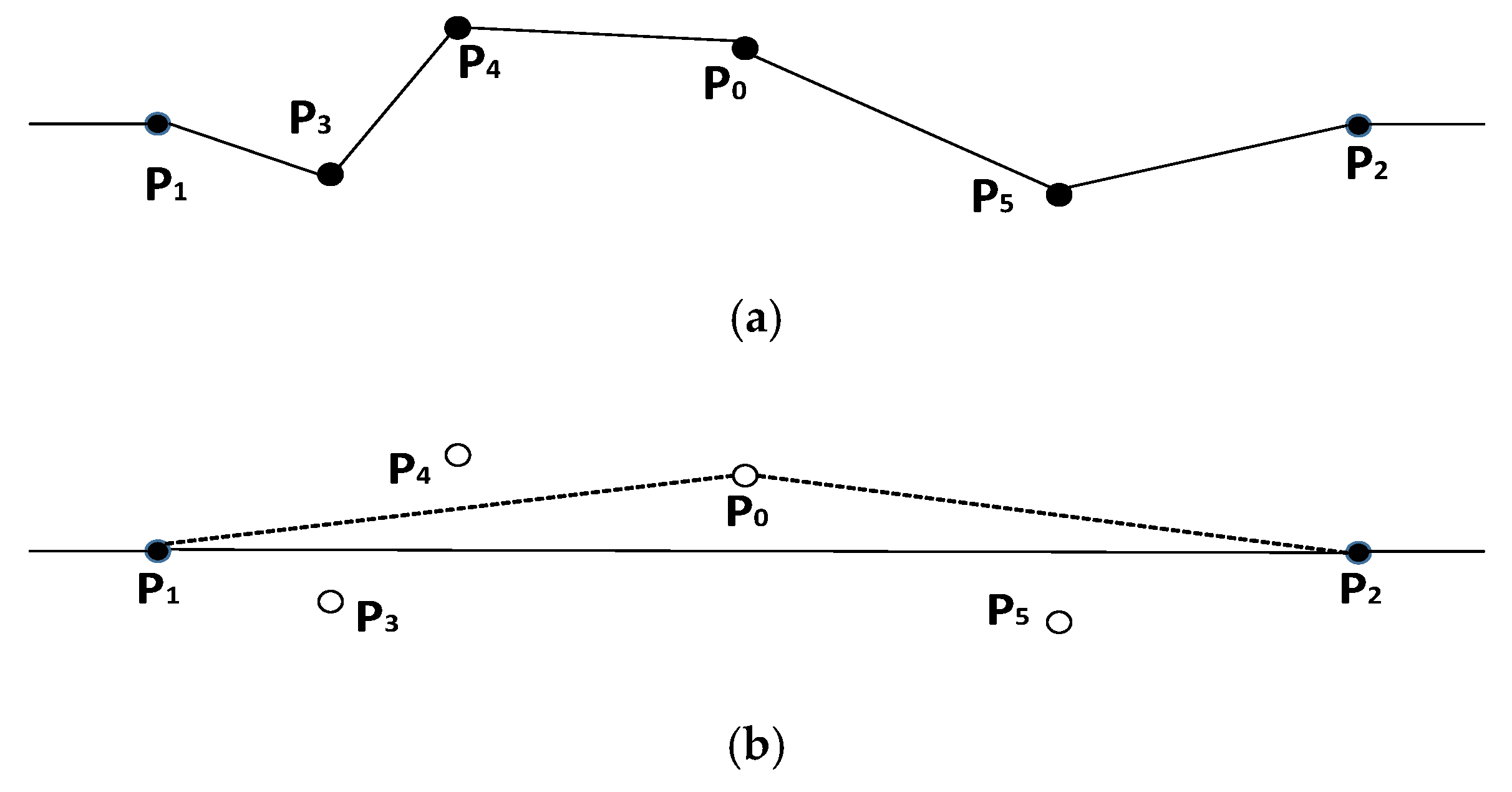
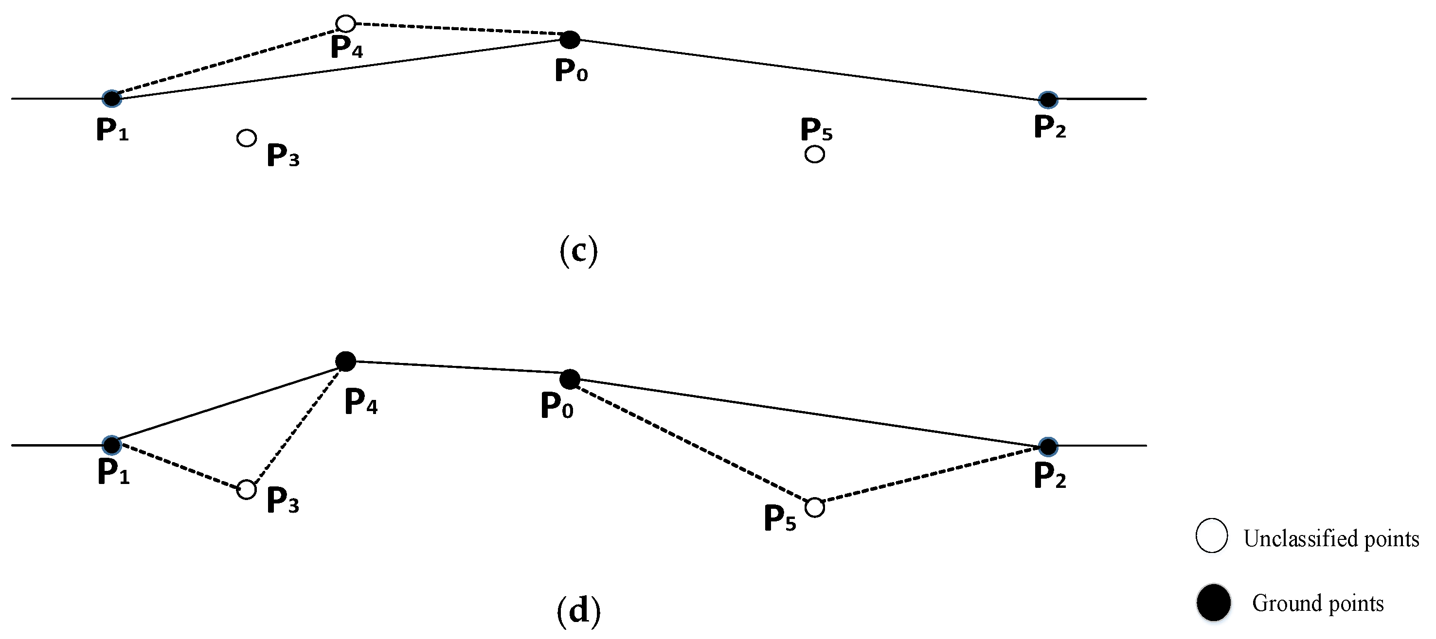
• In the initial densification stage, the TIN constructed by seed points only reflects the coarse ground surface shape. With the increase of points belonging to the TIN, the TIN is densified and is more approximate to the real terrain surface. In this stage, the calculated parameters include the angle and distance from the ground points to the TIN become smaller.
• In the second stage, the density of points belonging to TIN reaches a certain value. The horizontal distance between the added point and the vertex of the triangle becomes smaller, so that the standard variance of point clouds will cause that the calculated angle is beyond the angle threshold. The unclassified ground point will be rejected by the TIN. To guarantee that unclassified ground points can be added to the network as much as possible, the angle threshold should become larger in this stage.

Therefore, when we use the PTD algorithm to filter the point clouds with high density and standard variance, the distance threshold should be from large to small, whereas the angle threshold should be from large to small in the initial densification stage and then from small to large in the second stage. In this paper, we define this density as the standard variance interventional density ($DE{N}_{thr}$). When the density of point clouds belonging to TIN is higher than $DE{N}_{thr}$, the angle threshold should be increased so that the unclassified ground points as much as possible. Figure 1a,b shows the process of calculating $DE{N}_{thr}$. ∆ABC represents the real terrain surface, and the point P₀ is the unclassified ground point. The distance from point P₀ to ∆ABC is only caused by the standard variance of the point clouds, as the projected point P₃ of point P₀ is located at the center of ∆ABC. If the point P₀ can be added into the TIN, the area of the facet should be at least $3\sqrt{3}{\sigma }^2/{\tan }^2\alpha$; otherwise, this ground point is rejected. The density of the point clouds is the standard variance intervention density and is expressed as follows:

$$DE{N}_{thr}=k\times {\tan }^2\alpha /\left(3\sqrt{3}{\sigma }^2\right)$$

(3)

In Equation (3), $\sigma$ is the standard variance of the point clouds; $\alpha$ is the iteration angle which is specified before filtering; and k is called the density coefficient which is given by experience. In this paper, the parameter is 2.0–100.0. From Equation (3), we can see that $DE{N}_{thr}$ is inversely proportional to the standard variance of the point clouds. Since the density and the standard variance of the ALS data are small, the PTD algorithm can obtain good performance for the ALS data without considering the density and standard variance of the point clouds. However, for point clouds with high density and standard variance, such as the DIM point clouds, the type I error of the PTD algorithm may be very high when the PTD algorithm is used for filtering.

2.5. Our Improved PTD Algorithm

Based on the analysis in Section 2.4, this paper proposes an improved PTD algorithm considering the density and standard variance of point clouds. Figure 3 shows the entire workflow of the revised PTD algorithm. In Figure 3, the improved PTD algorithm mainly consists of three steps: (1) parameter specification and seed point selection; (2) iterative densification based on the densification strategy of the PTD algorithm; and (3) iterative densification of TIN based on multi-scales.

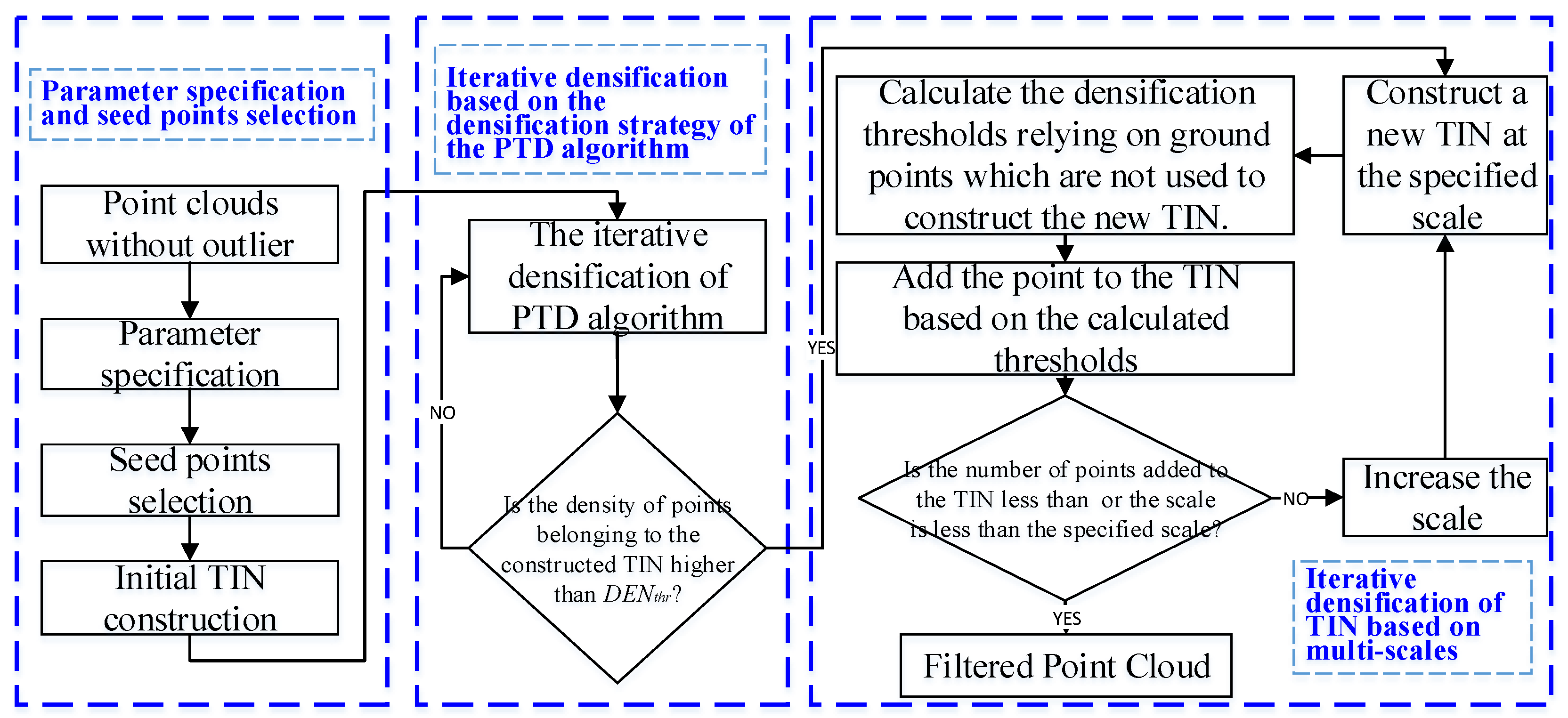
2.5.1. Parameter Specification and Seed Point Selection

In this section, we specify the initial densification parameters and select seed points according to Refs. [25,26]. The selected seed points are used to construct the initial TIN.

2.5.2. Iterative Densification Based on the Densification Strategy of the PTD Algorithm

Since the TIN constructed by seed points only contains a few points, the length of each edge of the facet is large. The standard variance of the point clouds has little impact on the filtering results. Hence, we can still apply the strategy of the PTD algorithm to densify the TIN in the initial densification stage. When the density of points belonging to the constructed TIN is higher than $DE{N}_{thr}$, the densification process moves into the next stage.

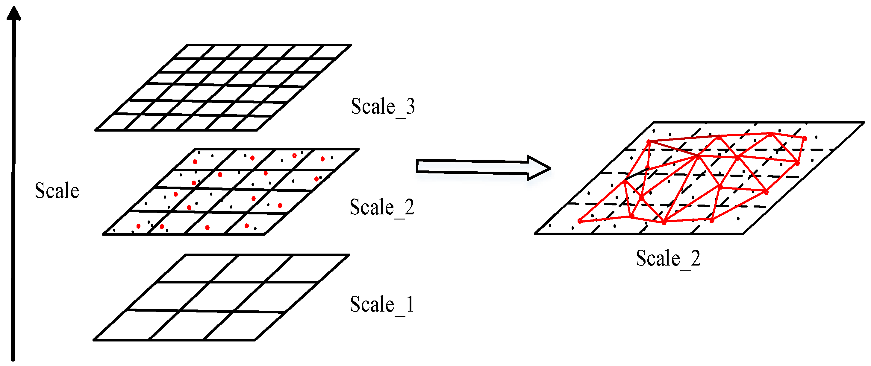
2.5.3. Iterative Densification of TIN Based on Multi-Scales

The distribution of points in the TIN is not uniform (e.g., the size of each facet in the TIN varies greatly). This leads to the fact that one set of densification thresholds cannot meet the densification requirements. To overcome the limitations, the points need to be resampled according to the specified scale. The resampled points are used to construct a new TIN where the distribution of points is roughly uniform. Specifically:

• Divide the survey region into grids according to the specified scale.
• Choose a point in a random grid, as shown with the red points in Figure 4.
• Construct the TIN using the selected points (the constructed TIN can be seen in Figure 4).

Therefore, the process of the iterative densification of TIN based on the multi-scales in the improved PTD algorithm can be summarized as follows:

• Divide ground points obtained in the third step into grids according to the specified scale and use the resampled points to construct a new TIN.
• Calculate the densification thresholds including angle and distance threshold.
• If both the calculated angle and distance values of an unclassified point are less than the calculated densification thresholds, this point is classified as a ground point; otherwise, it is an objective point. If the number of points added to the new TIN is less than $n$ or the given scale is less than $s_{thr}$, go to the fifth step; otherwise, go to the fourth step.
• Increase the scale (e.g., reduce the size of grid cell) and go to the first step.
• The filtering is finished and results are output.

In this paper, $n$ and $s_{thr}$ are 2000 and $1\mathrm{m}$, respectively. The key step of this process is how to calculate the densification thresholds. As shown in Figure 4, at Scale_2, the constructed TIN only contains a part of ground points. The angle and distance values from ground points which are not used for the construction of the new TIN reflect the angle and distance values from the unclassified ground points in the TIN at Scale_2. Based on this, a new strategy for calculating the densification thresholds is proposed here:

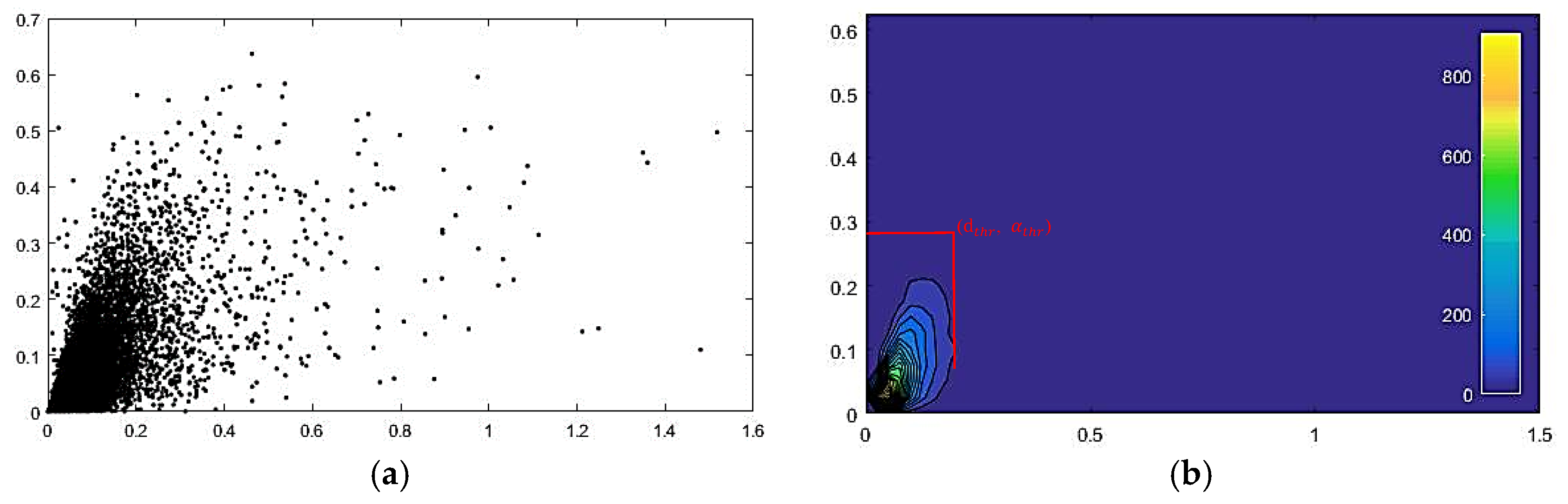
• Calculate the angle and distance values from ground points which are not used to construct the new TIN to this TIN.
• Project the calculated distance and angle values to a plane with the angle value on the vertical axis and the distance value on the horizontal axis, as shown in Figure 5a.
• Divide the two-dimensional planar into grids according to the specific size and calculate the number of points within each grid.
• Use the triangulation-based scattered data interpolation method [38] to generate a contour map. The corresponding maximum angle value and maximum distance value of the outer contour present the densification parameters shown in Figure 5b.

3. Experiments and Performance Evaluation

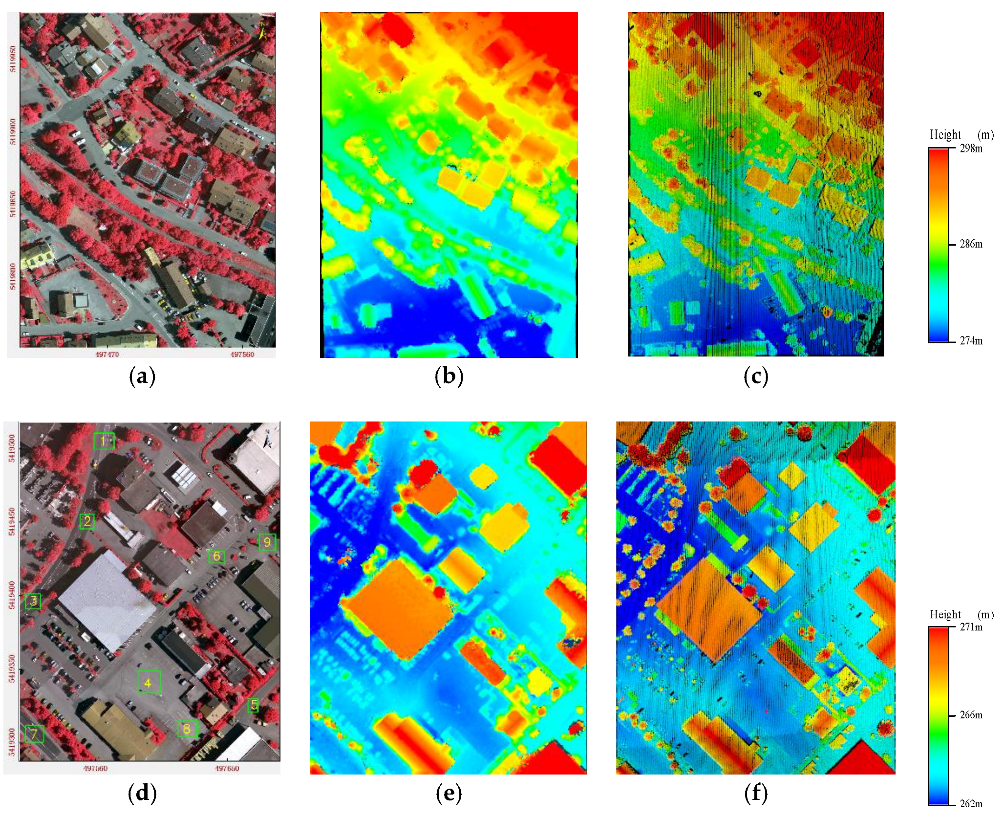
3.1. Data Description and Study Area

The performance of the proposed approach was tested on the Vaihingen dataset, which is published by international society for photogrammetry and remote sensing (ISPRS) Commission II/Working Group II/4 and has the real ground reference value. Two patches numbered 11 and 32 were selected for evaluation, where the patch numbered 11 is a slope area and the patch numbered 32 is a flat area. This dataset consists of two types of data: aerial images and ALS data. We used the commercial software PhotoScan [35] to generate the DIM points combining the supplied orientation parameters. The test datasets can be seen in Figure 6.

Table 1. The fundamental information of two test datasets.

Test Area	Long (m) $\times$ Width (m)	The Type of Data	The Number of Points	Density
11	$300\times 400$	DIM point clouds	1,678,370	$42.7/\mathrm{m}$2
		ALS data	164,452	$4.1/\mathrm{m}$2
32	$230\times 178.2$	DIM point clouds	1,477,565	$36.1/\mathrm{m}$2
		ALS data	275,679	$6.7/\mathrm{m}$2

shows the basic information of the test data. ISPRS gave the semantic labels of the two test areas. However, since ALS data and aerial images were obtained at different times, the real ground reference values need to be modified slightly by an operator.

The standard variance and density of point clouds are important parameters in our proposed algorithm. Before filtering, the standard variance of the point clouds should be calculated. As shown in Figure 6d, nine planar patches were selected. Equation (1) was used to calculate the standard variance of each patch, and the average standard variance of nine patches presents the standard variance of the point clouds. The standard variances of the two types of point clouds can be seen in

Table 2. The calculated standard variance of two types of point clouds.

Selected Area	1	2	3	4	5	6	7	8	9	Average
The standard variance of the DIM point clouds (m)	0.077	0.053	0.089	0.073	0.07	0.055	0.061	0.054	0.063	0.066
The standard variance of the ASL data (m)	0.021	0.02	0.017	0.04	0.021	0.031	0.022	0.032	0.041	0.027

. In Table 2, the standard variances of the DIM point clouds and ALS data are $0.066\mathrm{m}$ and $0.027\mathrm{m}$, respectively. In this experiment, we defined the density coefficient $k$ as $10.0$. According to Equation (3), the standard variance intervention densities of ALS data and DIM point clouds are $29.2/\mathrm{m}$² and $4.9/\mathrm{m}$², respectively. Since the density of ALS data is far smaller than $29.2/\mathrm{m}$², we used the proposed method to filter the DIM point clouds and rarefied DIM point clouds, which were resampled according to the density of the ALS data, and used the PTD method to filter the DIM point clouds, the rarefied DIM point clouds and the ALS data.

3.2. Parameter Selection

Our improved PTD method has five key parameters in common with the classical PTD method. The values of these input parameters are dependent on the experienced judgment based on the site landscape. In this study, the values of all key input parameters were determined according to previous studies [25,26,27]. The detailed values of all parameters in the PTD and improved PTD methods are listed in

Table 3. The values of all input parameters in the PTD and improved PTD methods for two test areas.

Test Area	The Type of Data	The Initial Parameter in Filtering
		Grid Size/m	Terrain Angle/°	Max Angle/°	Max Distance/m	Minimum Edge Length/m
11	DIM point clouds	30	88	6	1.4	-
	ALS data	30	88	6	1.4	-
32	DIM point clouds	30	88	6	0.8	-
	ALS data	30	88	6	0.8	-

.

In this paper, we mainly focus on the process of iterative densification. To weaken the effect of seed points on filtering results, the seed points were selected by operators. The selected seed points for two test areas can be seen in Figure 7.

3.3. Performance Evaluation between the PTD Algorithm and Improved PTD Algorithm

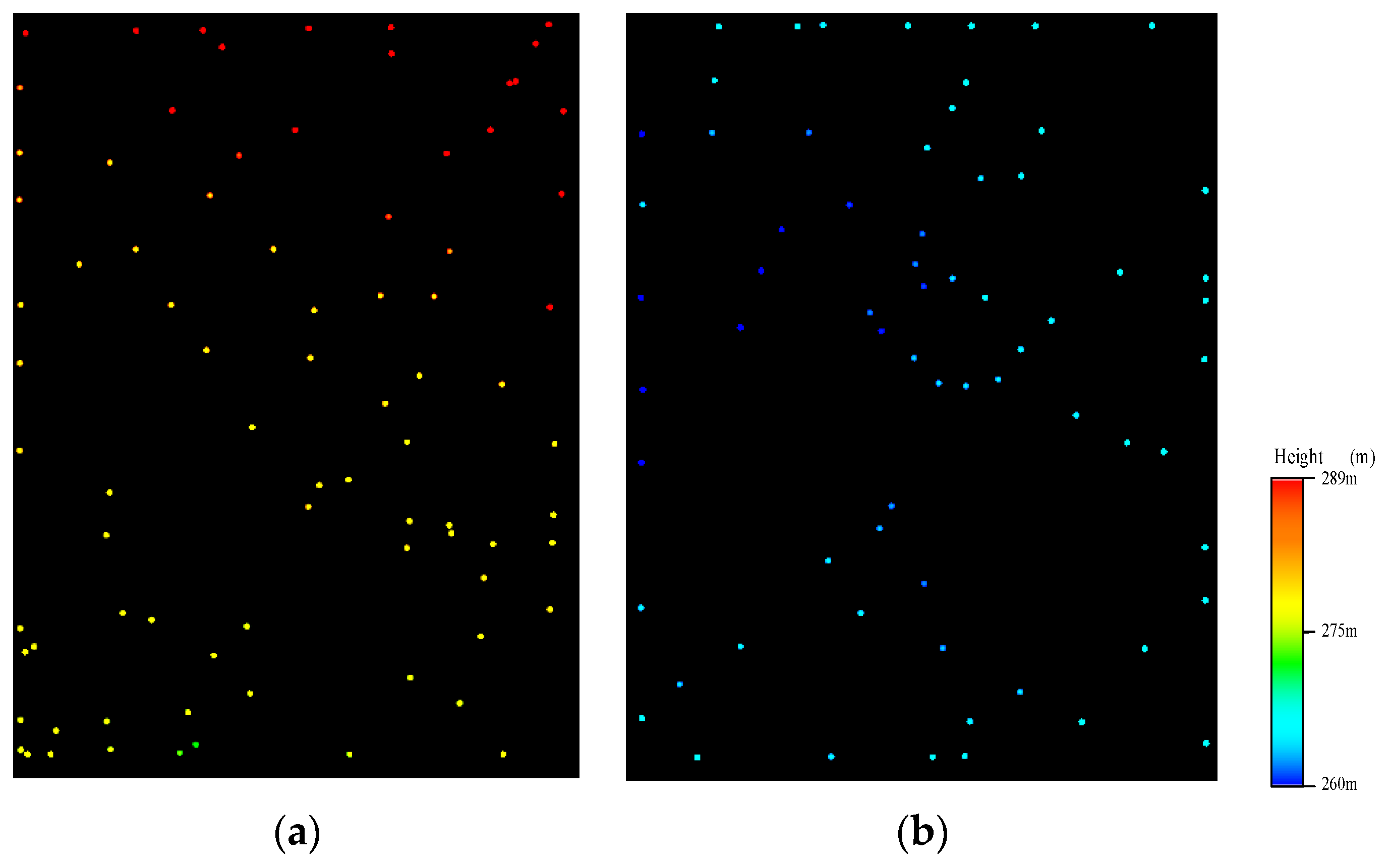
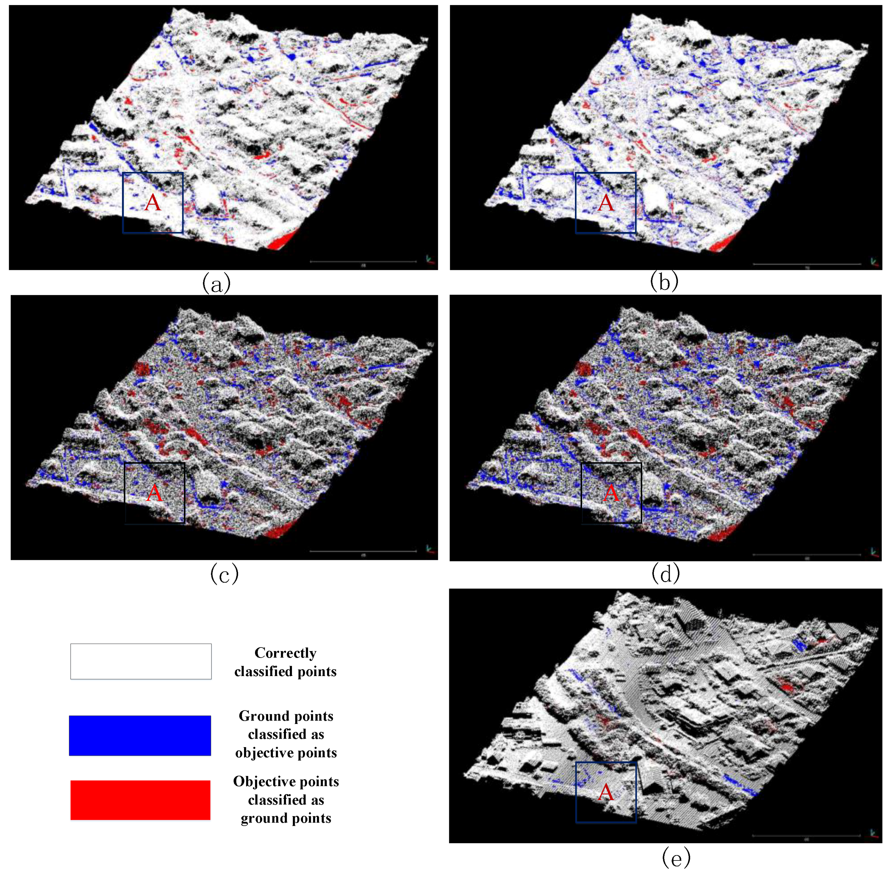
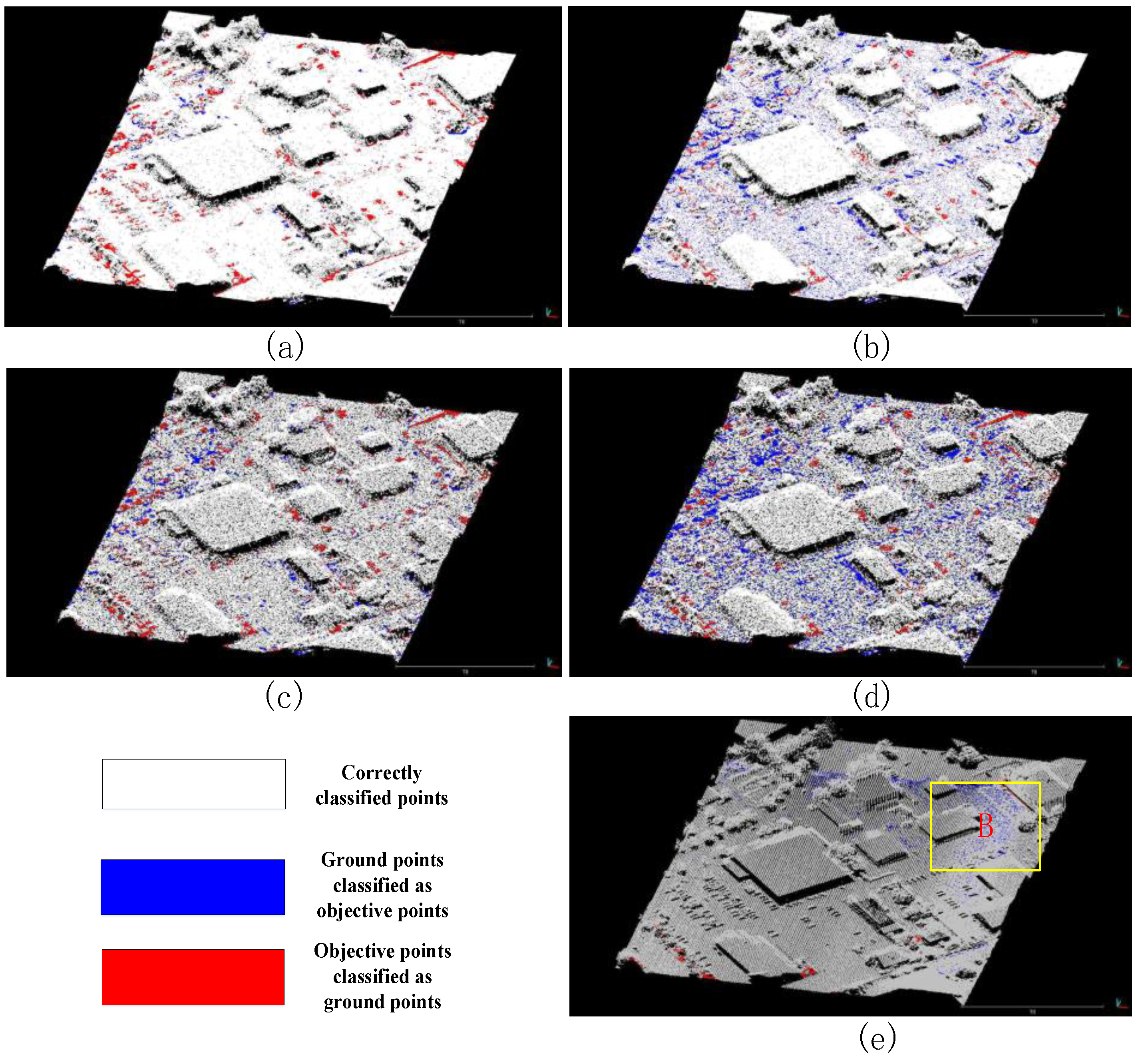
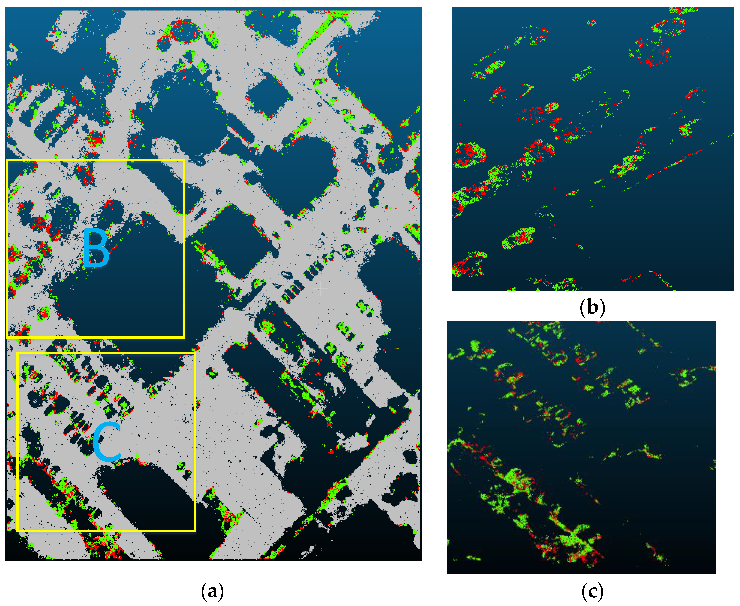
3.3.1. Qualitative Analysis

The qualitative analysis is made by visual inspection. Figure 8, Figure 9 and Figure 10 show the filtering results of two kinds of methods for the three types of data in two test areas. In Figure 8, Figure 9 and Figure 10, the size of the points from the ALS and rarefied DIM point clouds is larger than that of points from the DIM point cloud so that we can see the clear results of the PTD algorithm and improved PTD algorithm on the rarefied DIM point clouds and the ALS data. It is obvious that, compared with the PTD algorithm, the improved PTD algorithm has better performance for point clouds with high density and standard variance (e.g., the DIM point clouds and the rarefied DIM point clouds). Two factors hinder the performance of the PTD method:

• The standard variance of the DIM point clouds is higher than that of ALS data when the densities of point clouds are the same. We o concluded this because the comparison of the filtering results of the PTD method for the rarefied DIM point clouds and the ALS data in two test areas indicates that the high standard variance of point clouds damages the performance of the PTD algorithm.
• The high density of DIM point clouds can also damage the performance of the PTD algorithm when the standard variances of point clouds are the same. The filtering results of the PTD method for the DIM point clouds and the rarefied DIM point clouds confirm this conclusion. In fact, the type I errors of the PTD method on the rarefied DIM point clouds are 7.4% and 9.6% in the two test areas, respectively, and are lower than that of the PTD method on the original DIM point clouds. The above analysis agrees with previous studies (see Section 2.3), which demonstrates that the high standard variance and density of point clouds impact the performance of the PTD method.

3.3.2. Quantitative Analysis

Three types of errors, proposed by Sithole and Vosselman [11], namely type I errors, type II errors, and total errors, were used to quantitatively analyze the performance of the two filtering algorithms. Type I error is the ratio of ground points misclassified as non-ground points, whereas type II error is the percentage of non-ground points misclassified as ground points, and total error is the ratio of all misclassified points. The expressions of type I error, type II error and total error are:

$$TypeErro{r}_I=c/\left(a+c\right)\times 100\%$$

(4)

$$TypeErro{r}_{II}=d/\left(b+d\right)\times 100\%$$

(5)

$$TypeErro{r}_T=\left(c+d\right)/\left(a+b+c+d\right)\times 100\%$$

(6)

where a represents the number of ground points, b represents the number of non-ground points, c presents the number of ground points which were wrongly classified as non-ground points, and d presents the number of off-ground points which were incorrectly classified as ground points. Three types of errors of the PTD and improved PTD methods on three types of point clouds in two testing areas can be seen in

Table 4. The values of three types of errors of the PTD method and improved PTD method on three types of point clouds in two test areas.

Test Area	Type of Data	PTD-Type of Error			Improved PTD-Type of Error
		I (%)	II (%)	Total (%)	I (%)	II (%)	Total (%)
Area 11	DIM data	11.09	9.73	10.74	5.52	11.62	7.43
	ALS data	0.75	1.7	1.18	-	-	-
	Rarefied DIM data	7.4	18.68	11.06	4.92	19.48	10.03
Area 32	DIM data	12.52	6.2	9.94	3.03	7.3	5.08
	ALS data	8.06	0.73	4.26	-	-	-
	Rarefied DIM data	9.6	10.4	9.96	3.37	11.6	7.53

.

The statistical results in Table 4 indicate that both filtering algorithms can achieve a relatively good filter performance, and the maximum total error is less than 11.06% for the two test datasets. Compared with the DIM point clouds and rarefied DIM point clouds, the PTD algorithm can obtain the best performance on the ALS data. This indicates that both the high density and high standard variance of point clouds can damage the performance of the PTD algorithm. Table 4 presents an interesting phenomenon: the type II errors of the PTD method on the rarefied DIM point clouds is higher than that of the PTD method on the DIM point clouds. This is mainly because the density of the rarefied DIM point clouds is lower than that of the DIM point clouds. In fact, the high density of DIM points will reduce the percentage of points added to TIN when the PTD algorithm is used. The phenomenon that the type II errors of the PTD method on the rarefied DIM point cloud is higher than that of the PTD method on the DIM point clouds can explain why the type II errors of the improved PTD method on the rarefied DIM point clouds is higher than that of the improved PTD method on the DIM point clouds. In fact, the process of iterative densification of our proposed method consists of two stages. In the first stage, the process of iterative densification PTD algorithm is used. This introduces type II errors. Additionally, the type I errors of the improved PTD method on the rarefied DIM point clouds and DIM point clouds are almost the same.

In Table 4, the average values of the type I, type II and total errors of the PTD algorithm for the DIM point clouds are 11.81%, 7.97% and 10.34%, respectively, and the average of the type I, type II and total errors of the improved PTD algorithm for the DIM point clouds are 4.28%, 9.46% and 6.26%, respectively. Similarly, the average values of the type I, type II and total errors of the PTD algorithm for the rarefied DIM point clouds are 8.5%, 14.54% and 10.51%, respectively, and the average of the type I, type II and total errors of the improved PTD algorithm for the rarefied DIM point clouds are 4.15%, 15.54% and 8.78%, respectively. The results show that our proposed method can reduce the type I errors and total errors of point clouds with high density and standard variance efficiently.

Compared with the PTD algorithm, the improved algorithm increases the type II errors slightly. This is mainly because the angle threshold increases in the process of the iterative densification of TIN based on multi-scales in our proposed method. Although the type II errors increase in our proposed method, these errors have little effect on the generation of DSM. This is mainly because the change of distance threshold becomes small in the process of the iterative densification of TIN based on multi-scales. As shown in Figure 11, the distribution of wrongly classified objective points is almost the same in both the PTD algorithm and improved PTD algorithm. The added wrongly classified objective points of the improved PTD algorithm are still within the region where the wrongly classified objective points of the PTD algorithm are located. The improved PTD algorithm only densifies these regions by the larger angle threshold. Hence, our proposed method has a huge advantage in dealing with point clouds with high density and standard variance.

Notably, our proposed method has a disadvantage. The density coefficient $k$ in Equation (3) is hard to be estimated because the facets belonging to TIN are not all symmetrical triangles. This leads to calculating $DEN$_thr which decides whether our proposed method would be inaccurate. The area marked $\mathrm{B}$ in Figure 10 shows this example.

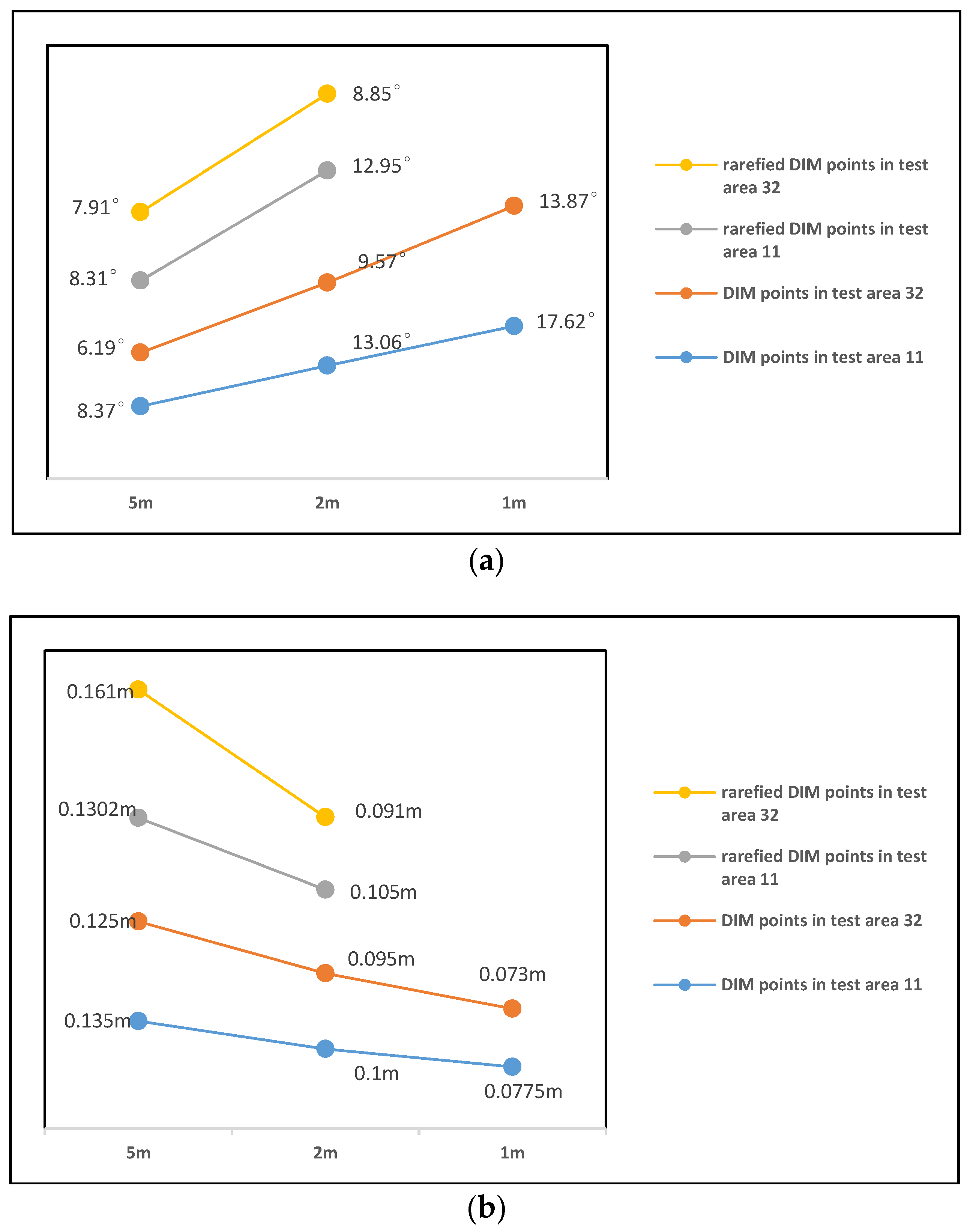
3.4. The Change of Iterative Densification Thresholds in the Improved PTD Algorithm

The biggest differences between the PTD method and our proposed method is the change of densification thresholds in the process of iterative densification. Figure 12 shows the change of densification thresholds including the angle and distance in the second densification stage of our proposed method on the DIM points and rarefied DIM points in two test areas.

Since the number of points added to TIN is less than 2000 in the second iterative densification stage of the proposed method for the rarefied DIM point clouds when the scale is $2\mathrm{m}$, the angle value and distance value is absence when the scale is $1\mathrm{m}$. Figure 12 shows that the distance value becomes smaller and the angle value becomes larger when the density of the points added to TIN is greater than $DEN$_thr. This change is in agreement with the description in Section 2.4.

4. Conclusions

Point clouds filtering is an essential processing step for the applications of point clouds, including ALS point clouds and DIM point clouds. In this paper, an improved PTD method is proposed. A dataset provided by ISPRS Commission II/Working Group II/4 was employed to verify our improved PTD method; moreover, the two reference samples from the sub-areas were used to calculate the accuracies of the proposed approach. The experimental results show that both our proposed method and the PTD method can achieve relatively good filter performance on different types of point clouds. However, the improved PTD method can obtain better performance on the point clouds with high density and standard variance compared with PTD method. Particularly, it may have significantly lower type I errors and total errors than the PTD algorithm, although it may have higher type II errors, which have little impact on the generation of DSM, which will reduce the cost of the following manual correction. This leads to our approach being extremely suitable for DIM point clouds which have high density and standard variance. However, this does not mean that our approach cannot be applied for ALS data. Since the density and standard variance of the ALS data are low, the calculated $DE{N}_{thr}$ is smaller than the density of the ALS data. The densification process of the improved PTD method will only stay in the first stage. Additionally, our approach is sensitive to the standard variance of point clouds. The incorrect standard variance will influence the estimation of $DEN$. _thr. Furthermore, the density is also given by experience. Future work will focus on improving the proposed filter to reduce the type II errors and how to calculate $DEN$_thr accurately.

References

1. Rau, J.Y.; Jhan, J.P.; Hsu, Y.C. Analysis of Oblique Aerial Images for Land Cover and Point Cloud Classification in an Urban Environment. IEEE Trans. Geosci. Remote Sens. 2015, 53, 1304–1319. [Google Scholar] [CrossRef]
2. Tang, H.; Brolly, M.; Zhao, F.; Strahler, A.H.; Schaaf, C.L.; Ganguly, S.; Zhang, G.; Dubayah, R. Deriving and validating Leaf Area Index (LAI) at multiple spatial scales through Lidar remote sensing: A case study in Sierra National Forest, CA. Remote Sens. Environ. 2014, 143, 131–141. [Google Scholar] [CrossRef]
3. Zhao, X.; Guo, Q.; Su, Y.; Xue, B. Improved progressive TIN densification filtering algorithm for airborne Lidar data in forested areas. ISPRS J. Photogramm. Remote Sens. 2016, 117, 79–91. [Google Scholar] [CrossRef]
4. Dahlke, D.; Linkiewicz, M.; Meissner, H. True 3D building reconstruction: Façade, roof and overhang modelling from oblique and vertical aerial imagery. Int. J. Image Data Fusion 2015, 6, 314–329. [Google Scholar] [CrossRef]
5. Sithole, G.; Vosselman, G. Experimental comparison of filter algorithms for bare-Earth extraction from airborne laser scanning point clouds. ISPRS J. Photogramm. Remote Sens. 2004, 59, 85–101. [Google Scholar] [CrossRef]
6. Hu, H.; Ding, Y.; Zhu, Q.; Wu, B.; Lin, H.; Du, Z.; Zhang, Y.; Zhang, Y. An adaptive surface filter for airborne laser scanning point clouds by means of regularization and bending energy. ISPRS J. Photogramm. Remote Sens. 2014, 92, 98–111. [Google Scholar] [CrossRef]
7. Kraus, K.; Pfeifer, N. Determination of terrain models in wooded areas with airborne laser scanner data. ISPRS J. Photogramm. Remote Sens. 1998, 53, 193–203. [Google Scholar] [CrossRef]
8. Zhang, J.; Lin, X. Filtering airborne Lidar data by embedding smoothness-constrained segmentation in progressive TIN densification. ISPRS J. Photogramm. Remote Sens. 2013, 81, 44–59. [Google Scholar] [CrossRef]
9. Sithole, G. Filtering of laser altimetry data using a slope adaptive filter. Int. Arch. Photogramm. Remote Sens. Spat. Inf. Sci. 2001, 34, 203–210. [Google Scholar]
10. Susaki, J. Adaptive slope filtering of airborne Lidar data in urban areas for digital terrain model (DTM) generation. Remote Sens. 2012, 4, 1804–1819. [Google Scholar] [CrossRef] [Green Version]
11. Vosselman, G. Slope based filtering of laser altimetry data. Int. Arch. Photogramm. Remote Sens. 2000, 33, 935–942. [Google Scholar]
12. Lohmann, P. Segmentation and filtering of laser scanner digital surface models. Int. Arch. Photogramm. Remote Sens. Spat. Inf. Sci. 2002, 34, 311–316. [Google Scholar]
13. Shen, J.; Liu, J.; Lin, X.; Zhao, R. Object-based classification of airborne light detection and ranging point clouds in human settlements. Sens. Lett. 2012, 10, 221–229. [Google Scholar] [CrossRef]
14. Sithole, G.; Vosselman, G. Filtering of airborne laser scanner data based on segmented point clouds. In Proceedings of the Laser Scanning 2005, Enschede, The Netherlands, 12–15 September 2005. [Google Scholar]
15. Yan, M.; Blaschke, T.; Liu, Y.; Wu, L. An object-based analysis filtering algorithm for airborne laser scanning. Int. J. Remote Sens. 2012, 33, 7099–7116. [Google Scholar] [CrossRef]
16. Glenn, N.; Spaete, L.; Sankey, T.; Derryberry, D.; Hardegree, S.; Mitchell, J. Errors in LiDAR-derived shrub height and crown area on sloped terrain. J. Arid Environ. 2011, 75, 377–382. [Google Scholar] [CrossRef]
17. Sankey, T.T.; Bond, P. LiDAR-based classification of sagebrush community types. Rangel. Ecol. Manag. 2011, 64, 92–98. [Google Scholar] [CrossRef]
18. Murphy, P.N.; Ogilvie, J.; Meng, F.R.; Arp, P. Stream network modelling using Lidar and photogrammetric digital elevation models: A comparison and field verification. Hydrol. Process. 2008, 22, 1747–1754. [Google Scholar] [CrossRef]
19. Chen, Q.; Gong, P.; Baldocchi, D.; Xie, G. Filtering airborne laser scanning data with morphological methods. Photogramm. Eng. Remote Sens. 2007, 73, 175–185. [Google Scholar] [CrossRef]
20. Hui, Z.; Hu, Y.; Yevenyo, Y.Z.; Yu, X. An Improved Morphological Algorithm for Filtering Airborne Lidar Point Cloud Based on Multi-Level Kriging Interpolation. Remote Sens. 2016, 8, 35. [Google Scholar] [CrossRef]
21. Pingel, T.J.; Clarke, K.C.; McBride, W.A. An improved simple morphological filter for the terrain classification of airborne LIDAR data. ISPRS J. Photogramm. Remote Sens. 2013, 77, 21–30. [Google Scholar] [CrossRef]
22. Zhang, K.; Chen, S.-C.; Whitman, D.; Shyu, M.-L.; Yan, J.; Zhang, C. A progressive morphological filter for removing non ground measurements from airborne LIDAR data. IEEE Trans. Geosci. Remote Sens. 2003, 41, 872–882. [Google Scholar] [CrossRef]
23. Kobler, A.; Pfeifer, N.; Ogrinc, P.; Todorovski, L.; Oštir, K.; Dzěroski, S. Repetitive interpolation: A robust algorithm for DTM generation from Aerial Laser Scanner Data in forested terrain. Remote Sens. Environ. 2007, 108, 9–23. [Google Scholar] [CrossRef]
24. Polat, N.; Uysal, M.; Toprak, A.S. An investigation of DEM generation process based on Lidar data filtering, decimation, and interpolation methods for an urban area. Measurement 2015, 75, 50–56. [Google Scholar] [CrossRef]
25. Axelsson, P. DEM Generation from Laser Scanner Data Using Adaptive TIN Models. Int. Arch. Photogramm. Remote Sens. 2000, 33, 110–117. [Google Scholar]
26. Lin, X.; Zhang, J. Segmentation-based filtering of airborne Lidar point clouds by progressive densification of terrain segments. Remote Sens. 2014, 6, 1294–1326. [Google Scholar] [CrossRef]
27. Wang, H.; Wang, S.; Chen, Q.; Jin, W.; Sun, M. An improved filter of progressive TIN densification for LiDAR point cloud data. Wuhan Univ. J. Nat. Sci. 2015, 20, 362–368. [Google Scholar] [CrossRef]
28. Nie, S.; Wang, C.; Dong, P.; Xi, X.; Luo, S.; Qinetl, H. A revised progressive TIN densification for filtering airborne Lidar data. Measurement 2017, 104, 70–77. [Google Scholar] [CrossRef]
29. Zhang, J.; Lin, X.; Ning, X. SVM-Based Classification of Segmented Airborne Lidar Point Clouds in Urban Areas. Remote Sens. 2013, 5, 3749–3775. [Google Scholar] [CrossRef]
30. Yilmaz, C.S.; Gungor, O. Comparison of the performances of ground filtering algorithms and DTM generation from a UAV-based point cloud. Geocarto Int. 2016, 32, 1–41. [Google Scholar]
31. Zhang, Z.; Gerke, M.; Vosselman, G.; Yang, M.Y. Filtering Photogrammetric Point Clouds Using Standard Lidar Filters Towards Dtm Generation. ISPRS Ann. Photogramm. Remote Sens. Spat. Inf. Sci. 2018, 2, 319–326. [Google Scholar] [CrossRef]
32. Maltezos, E.; Ioannidis, C. Automatic Detection of Building Points from Lidar and Dense Image Matching Point Clouds. In Proceedings of the ISPRS Geospatial Week 2015, 28 September–2 October 2015; pp. 39–41. [Google Scholar]
33. Nex, F.; Remondino, F. Automatic Roof Outlines Reconstruction from Photogrammetric DSM. ISPRS Ann. Photogramm. Remote Sens. Spat. Inf. Sci. 2012, 1, 257–262. [Google Scholar] [CrossRef]
34. Gerke, M.; Xiao, J. Fusion of airborne laser scanning point clouds and images for supervised and unsupervised scene classification. ISPRS J. Photogramm. Remote Sens. 2014, 87, 78–92. [Google Scholar] [CrossRef]
35. Agisoft. Agisoft PhotoScan. 2018. Available online: http://www.agisoft.ru/products/photoscan/professional/ (accessed on 25 August 2018).
36. Dong, Y.Q.; Zhang, L.; Cui, X.M.; Ai, H.B. An Automatic Filter Algorithm for Dense Image Matching Point Clouds. ISPRS Int. Arch. Photogramm. Remote Sens. Spat. Inf. Sci. 2017, 42, 703–709. [Google Scholar] [CrossRef]
37. Mann, P.S. Introductory Statistics, 7th ed.; John Wiley and Sons Inc.: New York, NY, USA, 2010. [Google Scholar]
38. The Math Works, Inc. Interpolating Scattered Data. Available online: https://www.mathworks.com/help/matlab/math/int erpolating-scattered-data.html (accessed on 30 September 2018).
Figure 1. The densification of point clouds in the minimum edge mode: (a) the top view of unclassified ground points located near the center of the TIN facet; (b) the main view of unclassified ground points located near the center of the TIN facet; (c) the top view of unclassified ground points located near a vertex of the TIN facet; and (d) the main view of unclassified ground points located near a vertex of the TIN facet.
Ijgi 07 00409 g001
Figure 2. The process of point cloud densification in the non-minimum edge mode: (a) the true ground surface; and (bd) the process of the densification of TIN.
Ijgi 07 00409 g002aIjgi 07 00409 g002b
Figure 3. The flowchart of the improved progressive triangular irregular network densification algorithm.
Ijgi 07 00409 g003
Figure 4. The process of the iterative densification of TIN based on multi-scales.
Ijgi 07 00409 g004
Figure 5. Illustration of selecting densification thresholds: (a) the distribution of ground points which don’t construct the TIN on the threshold plane; (b) the generated contour map.
Ijgi 07 00409 g005
Figure 6. The test data in two areas: test area 11 ((a) orthoimagery; (b) dense image matching (DIM) point clouds; and (c) ALS data); and test area 32 ((d) orthoimagery; (e) DIM point clouds; and (f) ALS data).
Ijgi 07 00409 g006
Figure 7. The selected seed points: (a) the selected seed points in area 11; and (b) the selected seed points in area 32.
Ijgi 07 00409 g007
Figure 8. Filtering results of different types of point clouds in test area 11: (a) the filtering results of the proposed method for the DIM point clouds; (b) the filtering results of the PTD method for the DIM point clouds; (c) the filtering results of the proposed method for the rarefied DIM point clouds; (d) the filtering results of the PTD method for the rarefied DIM point clouds; (e) the filtering results of the PTD method for the ALS point clouds.
Ijgi 07 00409 g008
Figure 9. Areas marked A in Figure 8 are magnified: (a) the filtering results of the PTD method for the DIM point clouds; (b) the filtering results of the PTD method for the rarefied DIM point clouds; (c) the filtering results of the PTD method for the ALS point clouds; (d) the filtering results of the proposed method for the DIM point clouds; (e) the filtering results of the proposed method for the rarefied DIM point clouds.
Ijgi 07 00409 g009
Figure 10. Filtering results of different types of point clouds in test area 32: (a) the filtering results of the proposed method for the DIM point clouds; (b) the filtering results of the PTD method for the DIM point clouds; (c) the filtering results of the proposed method for the rarefied DIM point clouds; (d) the filtering results of the PTD method for the rarefied DIM point clouds; (e) the filtering results of the PTD method for the ALS point clouds.
Ijgi 07 00409 g010
Figure 11. The distribution of type II errors of the PTD algorithm and improved PTD algorithm: green points are wrongly classified objective points in the PTD method and red points are wrongly classified objective points in the improved PTD method. In test area 32: (a) the entire distribution of objective points wrongly classified as ground points; and (b,c) the corresponding region of yellow rectangle labeled in (a).
Ijgi 07 00409 g011
Figure 12. The change of densification thresholds in the second iterative densification stage of the proposed method: (a) the change of the angle threshold at different scales; and (b) the change of the distance threshold at different scales.
Ijgi 07 00409 g012