The Effects of Land Use and Land Cover Geoinformation Raster Generalization in the Analysis of LUCC in Portugal


Abstract
:
1. LUC: Multiscale Framework, Geoinformation Availability, and Raster Generalization Process
1.1. LUC Changes: An Overview
1.2. LUC Geoinformation
1.3. LUC Geoinformation Generalization
2. Objectives
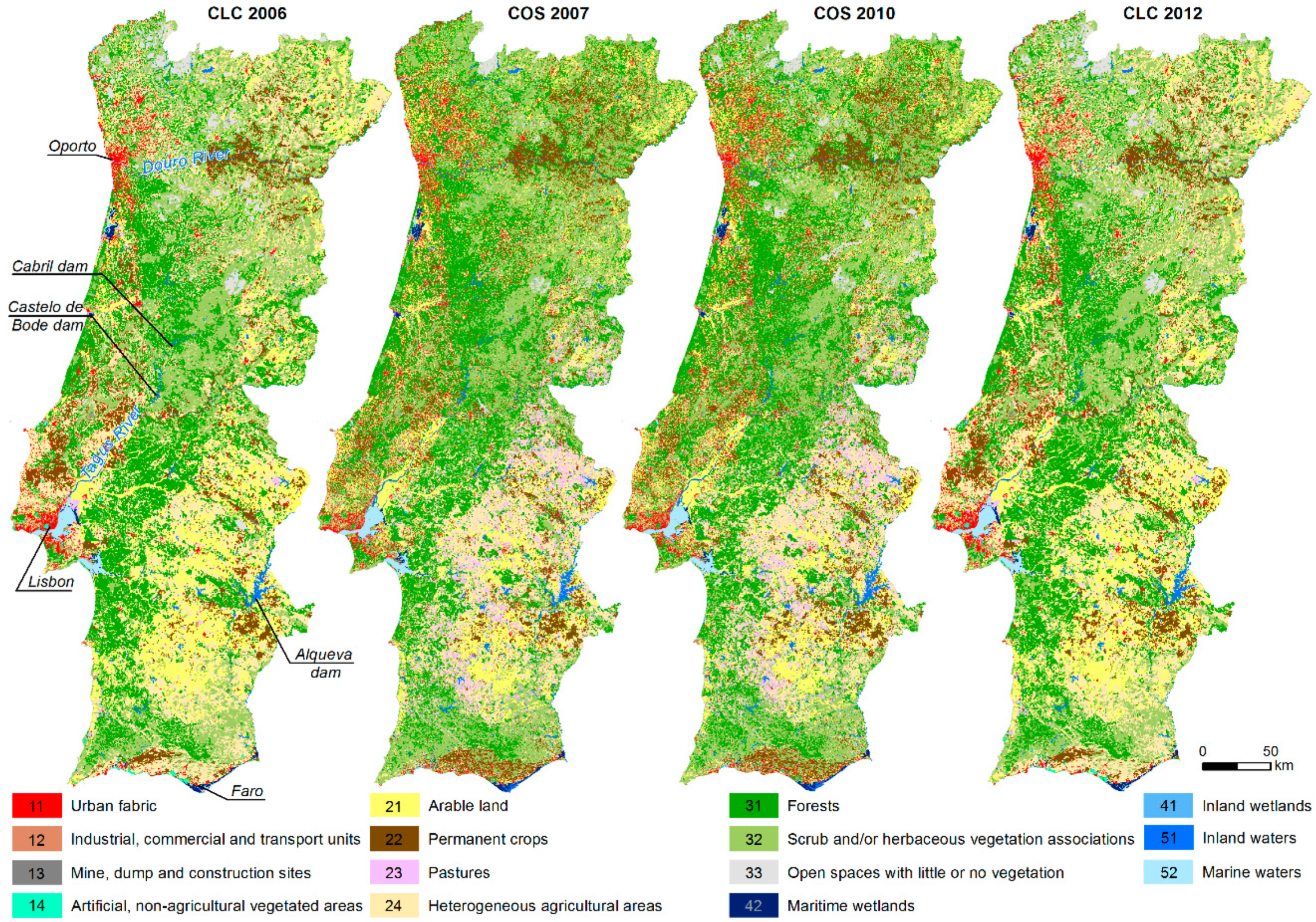
3. LUC of Portugal
4. Data, Tools, and Methods
4.1. LUC Geoinformation and Multispecifications
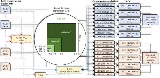
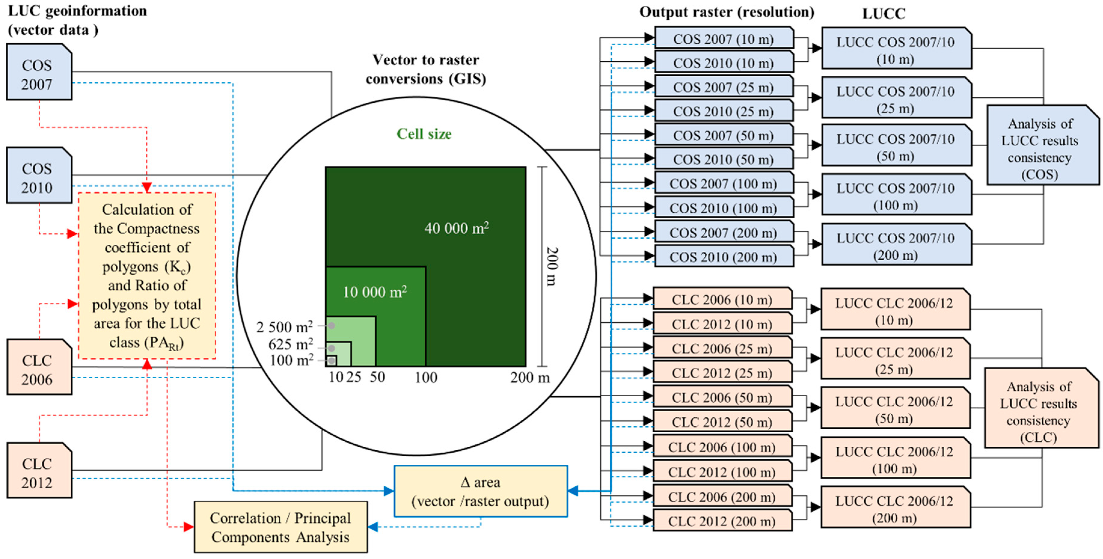
4.2. Tools and LUCC Methodology
5. Results and Discussion
5.1. Area of Mainland Portugal at Different Raster Resolutions
5.2. LUC at Different Raster Resolutions
5.3. LUCC at Different Raster Resolution Levels
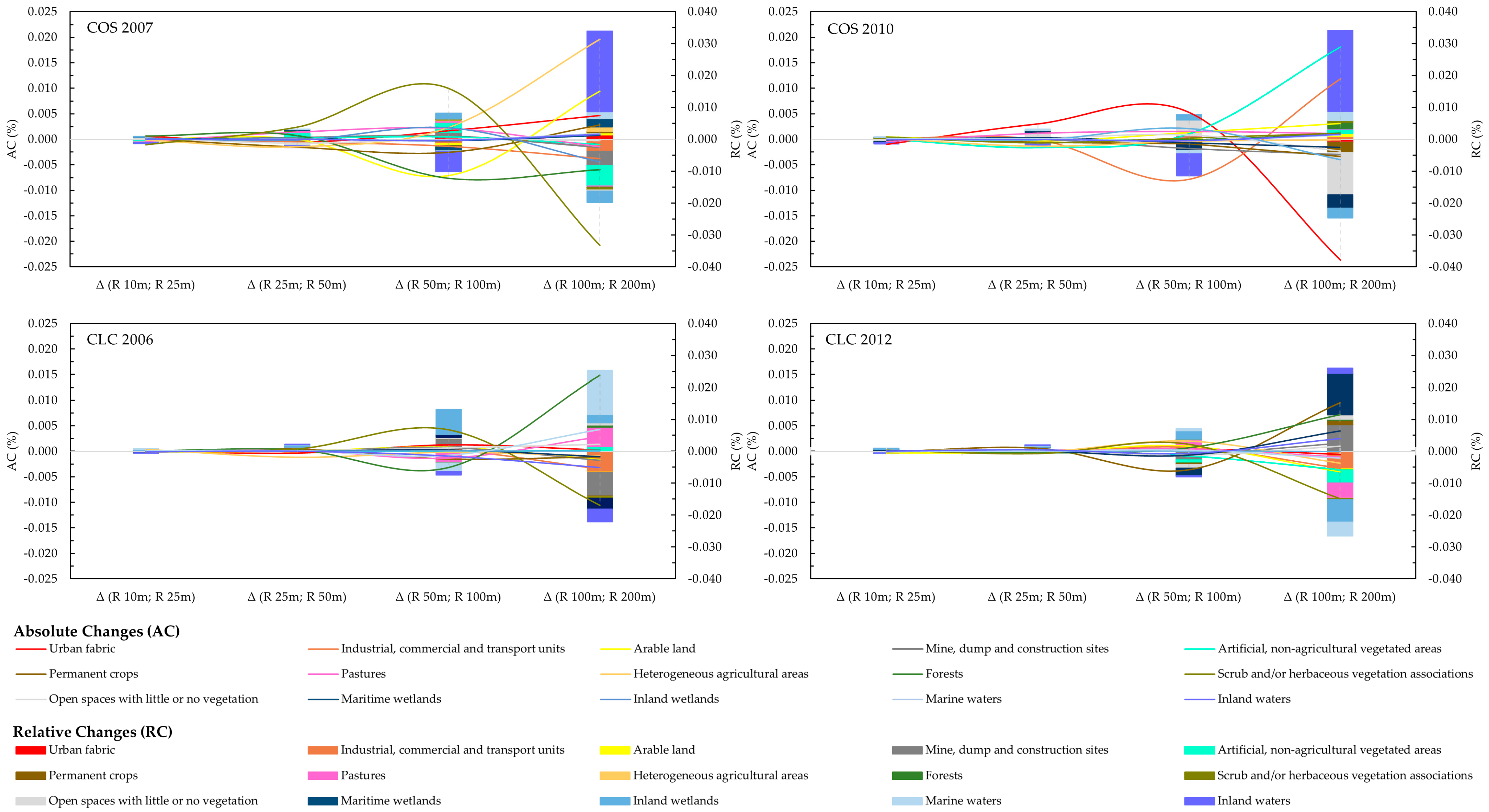
5.4. LUCC Variations
6. Conclusions
Author Contributions
Funding
Acknowledgments
Conflicts of Interest
References
- Ramankutty, N.; Graumlich, L.; Achard, F.; Alves, D.; Chhabra, A.; DeFries, R.S.; Foley, J.A.; Geist, H.; Houghton, R.A.; Goldewijk, K.K.; et al. Global Land-Cover Change: Recent Progress, Remaining Challenges. In Land-Use and Land-Cover Change Local Processes and Global Impacts; Lambin, E.F., Geist, H., Eds.; Springer: Berlin, Germany, 2006; pp. 9–70. [Google Scholar]
- Charney, J.; Stone, P.H.; Quirk, W.J. Drought in the Sahara: A biogeophysical feedback mechanism. Science 1975, 187, 434–435. [Google Scholar] [CrossRef] [PubMed]
- Otterman, J. Baring high-albedo soils by overgrazing: A hypothesized desertification mechanism. Science 1974, 186, 531–533. [Google Scholar] [CrossRef] [PubMed]
- Yang, X.; Ren, L.; Singh, V.P.; Liu, X.; Yuan, F.; Jiang, S.; Yong, B. Impacts of land use and land cover changes on evapotranspiration and runoff at Shalamulun River watershed, China. Hydrol. Res. 2012, 43, 23–37. [Google Scholar] [CrossRef]
- Song, W.; Deng, X. Land-use/land-cover change and ecosystem service provision in China. Sci. Total Environ. 2017, 576, 705–719. [Google Scholar] [CrossRef] [PubMed]
- Tasser, E.; Leitinger, G.; Tappeiner, U. Climate change versus land-use change—What affects the mountain landscapes more? Land Use Policy 2017, 60, 60–72. [Google Scholar] [CrossRef]
- Bebi, P.; Seidl, R.; Motta, R.; Fuhr, M.; Firm, D.; Krumm, F.; Conedera, M.; Ginzler, C.; Wohlgemuth, T.; Kulakowski, D. Changes of forest cover and disturbance regimes in the mountain forests of the Alps. For. Ecol. Manag. 2016, in press. [Google Scholar]
- Cebecauer, T.; Hofierka, J. The consequences of land-cover changes on soil erosion distribution in Slovakia. Geomorphology 2008, 98, 187–198. [Google Scholar] [CrossRef]
- Gebresamuel, G.; Singh, B.R.; Dick, Ø. Land-use changes and their impacts on soil degradation and surface runoff of two catchments of Northern Ethiopia. Acta Agric. Scand. Sect. B Plant Soil Sci. 2010, 60, 211–226. [Google Scholar] [CrossRef]
- Tadesse, L.; Suryabhagavan, K.V.; Sridhar, G.; Legesse, G. Land use and land cover changes and Soil erosion in Yezat Watershed, North Western Ethiopia. Int. Soil Water Conserv. Res. 2017, 5, 85–94. [Google Scholar] [CrossRef]
- Hartemink, A.E. Land use change in the tropics and its effect on soil fertility. In Proceedings of the 19th World Congress of Soil Science, Soil Solutions for a Changing World, Brisbane, Australia, 1–6 August 2010; World Congress of Soil Science: Brisbane, Australia, 2010; Volume 1990, pp. 55–58. [Google Scholar]
- Foley, J.A.; Ramankutty, N.; Brauman, K.A.; Cassidy, E.S.; Gerber, J.S.; Johnston, M.; Mueller, N.D.; O’Connell, C.; Ray, D.K.; West, P.C.; et al. Solutions for a cultivated planet. Nature 2011, 478, 337–342. [Google Scholar] [PubMed] [Green Version]
- Petz, K. Mapping and Modelling the Effects of Land Use and Land Management Change on Ecosystem Services: From Local Ecosystems and Landscapes to Global Biomes; Wageningen University: Wageningen, NL, USA, 2014. [Google Scholar]
- Fichera, C.R.; Modica, G.; Pollino, M. Land Cover classification and change-detection analysis using multi-temporal remote sensed imagery and landscape metrics. Eur. J. Remote Sens. 2012, 45, 1–18. [Google Scholar] [CrossRef] [Green Version]
- Carpio, A.J.; Oteros, J.; Tortosa, F.S.; Guerrero-Casado, J. Land use and biodiversity patterns of the herpetofauna: The role of olive groves. Acta Oecol. 2016, 70, 103–111. [Google Scholar] [CrossRef] [Green Version]
- European Union–Eurostat (Online Publications) Land Cover and Land Use. Available online: http://ec.europa.eu/eurostat/statistics-explained/index.php/Land_cover_and_land_use (accessed on 27 July 2018).
- EEA (European Environment Agency). Landscapes in Transition: An Account of 25 Years of Land Cover Change in Europe; EEA: Luxembourg, 2017. [Google Scholar]
- European Commission Land Use Change. Available online: https://ec.europa.eu/energy/en/topics/renewable-energy/biofuels/land-use-change (accessed on 30 June 2018).
- Meneses, B.M.; Vale, M.J.; Reis, R.; Saraiva, R. Metodologias para a avaliação das alterações do uso e ocupação do solo em Portugal Continental nas últimas três décadas. CIDADES Comunidades Territ. 2013, 27, 50–60. [Google Scholar] [CrossRef]
- Meneses, B.M.; Vale, M.J.; Reis, R. Uso e ocupação do solo. In Uso e Ocupação do Solo em Portugal Continental: Avaliação e Cenários Futuros, Projeto LANDYN; Direção Geral do Território, Ed.; Direção-Geral do Território: Lisboa, Portugal, 2014; pp. 16–52. [Google Scholar]
- DGT (Directorate General of Traffic). LANDYN—Alterações de Uso e Ocupação do Solo em Portugal Continental: Caracterização, Forças Motrizes e Cenários Futuros. Relatório Anual 2012–2013; DGT: Lisboa, Portugal, 2013.
- Meneses, B.M.; Reis, E.; Pereira, S.; Vale, M.; Reis, R. Understanding Driving Forces and Implications Associated with the Land Use and Land Cover Changes in Portugal. Sustainability 2017, 9, 351. [Google Scholar] [CrossRef]
- Meneses, B.M.; Vale, M.J.; Reis, R.; Marrecas, P.; Barreira, E. Metodologias para a avaliação do uso e ocupação do solo em diferentes épocas. In Uso e Ocupação do Solo em Portugal Continental: Avaliação e Cenários Futuros, Projeto LANDYN; DGT, Ed.; Direção-Geral do Território: Lisboa, Portugal, 2014; pp. 5–16. [Google Scholar]
- Nunes, V. Comparação Entre Cartografias de Ocupação e ou Uso do Solo Para a Produção de um Mapa de Incerteza Temática. Ph.D. Thesis, Instituto Superior de Estatística e Gestão de Informação da Universidade Nova de Lisboa, Lisbon, Portugal, 2008. [Google Scholar]
- IGP. Carta de Uso e Ocupação do Solo de Portugal Continental para 2007 (COS2007), 1st ed.; Memória Descritiva; Instituto Geográfico Português/Direção Geral do Território: Lisboa, Portugal, 2010. [Google Scholar]
- Gil, A.; Abadi, M. Using very high resolution satellite imagery for land cover mapping in Pico da Vara nature reserve (S. Miguel Island, Archipelago of the Azores, Portugal). In Proceedings of the 2015 IEEE International Geoscience and Remote Sensing Symposium (IGARSS), Milan, Italy, 26–31 July 2015; pp. 3329–3332. [Google Scholar]
- Santos, T.; Tenedório, J.A.; Rocha, J.; Encarnação, S. SATSTAT: Exploratory Analysis of Envisat-MERIS Data for Land Cover Mapping of Portugal in 2003. In Proceedings of the 14th European Colloquium on Theoretical and Quantitative Geography, Setembro, Portugal, 28–30 September 2005. [Google Scholar]
- Encarnação, S.; Gaudiano, M.; Santos, F.C.; Tenedório, J.A.; Pacheco, J.M. Fractal cartography of urban areas. Sci. Rep. 2012, 2, 527. [Google Scholar] [CrossRef] [PubMed]
- Vale, M.J.; Reis, R.; Meneses, B.M. A caraterização do uso e ocupação do solo de Portugal Continental. In Uso e Ocupação do Solo em Portugal Continental: Avaliação e Cenários Futuros, Projeto LANDYN; DGT, Ed.; Direção-Geral do Território: Lisboa, Portugal, 2014; pp. 1–5. [Google Scholar]
- Meneses, B.M. Analysis of Land Use and Land Cover Changes in the Valley of the Varosa (Portugal) by Landsat-TM Images and its Influence on Soil Conservation. GeoFocus 2013, 13, 270–290. (In Portuguese) [Google Scholar]
- ESRI ArcGIS Help Library. Available online: http://resources.arcgis.com/en/help/main/10.1/index.html#//001200000030000000 (accessed on 31 October 2017).
- Roy, D.P.; Wulder, M.A.; Loveland, T.R.; Woodcock, C.E.; Allen, R.G.; Anderson, M.C.; Helder, D.; Irons, J.R.; Johnson, D.M.; Kennedy, R.; et al. Landsat-8: Science and product vision for terrestrial global change research. Remote Sens. Environ. 2014, 145, 154–172. [Google Scholar] [CrossRef]
- Mandanici, E.; Bitelli, G. Preliminary comparison of sentinel-2 and landsat 8 imagery for a combined use. Remote Sens. 2016, 8, 1014. [Google Scholar] [CrossRef]
- Ma, L.; Cheng, L.; Li, M.; Liu, Y.; Ma, X. Training set size, scale, and features in Geographic Object-Based Image Analysis of very high resolution unmanned aerial vehicle imagery. ISPRS J. Photogramm. Remote Sens. 2015, 102, 14–27. [Google Scholar] [CrossRef]
- Senthilnath, J.; Kandukuri, M.; Dokania, A.; Ramesh, K.N. Application of UAV imaging platform for vegetation analysis based on spectral-spatial methods. Comput. Electron. Agric. 2017, 140, 8–24. [Google Scholar] [CrossRef]
- Fröhlich, B.; Bach, E.; Walde, I.; Hese, S.; Schmullius, C.; Denzler, J. Land Cover Classification of Satellite Images Using Contextual Information. ISPRS Ann. Photogramm. Remote Sens. Spat. Inf. Sci. 2013, 3, w1. [Google Scholar] [CrossRef]
- Carleer, A.P.; Debeir, O.; Wolff, E. Assessment of very high spatial resolution satellite image segmentations. Photogramm. Eng. Remote Sens. 2005, 71, 1285–1294. [Google Scholar] [CrossRef]
- Bai, X.; Sharma, R.C.; Tateishi, R.; Kondoh, A.; Wuliangha, B.; Tana, G. A Detailed and High-Resolution Land Use and Land Cover Change Analysis over the Past 16 Years in the Horqin Sandy Land, Inner Mongolia. Math. Probl. Eng. 2017, 2017. [Google Scholar] [CrossRef]
- Meneses, B.M.; Reis, E.; Vale, M.J.; Reis, R. Modeling land use and land cover changes in Portugal: A multi-scale and multi-temporal approach. Finisterra 2018. [Google Scholar] [CrossRef]
- Veregin, H. Data Quality Measurement and Assessment; National Centre for Geographic Information and Analysis, University of California at Santa Barbara: Santa Barbara, CA, USA, 1998. [Google Scholar]
- Veregin, H.; Lanter, D.P. Data-quality enhancement Techniques in layer-based Geographic Information Systems. Comput. Environ. Urban Syst. 1995, 19, 23–36. [Google Scholar] [CrossRef]
- Goodchild, M.F.; Li, L. Assuring the quality of volunteered geographic information. Spat. Stat. 2012, 1, 110–120. [Google Scholar] [CrossRef]
- Comber, A.; See, L.; Fritz, S.; Van Der Velde, M.; Perger, C.; Foody, G. Using control data to determine the reliability of volunteered geographic information about land cover. Int. J. Appl. Earth Obs. Geoinf. 2013, 23, 37–48. [Google Scholar] [CrossRef] [Green Version]
- Droj, G.; Suba, S.; Buba, A. Modern techniques for evaluation of spatial data quality. RevCAD J. Geod. Cadastre 2010, 265–272. [Google Scholar]
- Huisman, O.; de By, R.A. Principles of Geographic Information Systems; Huisman, O., de By, R.A., Eds.; International Institute for Geo-Information Science and Earth Observation: Enschede, The Netherlands, 2009. [Google Scholar]
- Jaakkola, O. Quality of multiscale land cover data. In Geographical Information ’97, Proceedings of the Third Joint European Conference & Exhibition on Geographical Information, Vienna, Austria, 16–18 April 1997; Hodgson, S., Rumor, M., Harts, J.J., Eds.; IOS Press: Vienna, Austria, 1997; pp. 335–344. [Google Scholar]
- Raposo, P.; Brewer, C.A.; Sparks, K. An impressionistic cartographic solution for base map land cover with coarse pixel data. Cartogr. Perspect. 2016, 83, 5–21. [Google Scholar] [CrossRef]
- Raposo, P.; Samsonov, T. Towards general theory of raster data generalization. In Proceedings of the 17th ICA Workshop on Generalisation and Multiple Representation, Vienna, Austria, 23 September 2014; p. 10. [Google Scholar]
- Shea, K.S.; McMaster, R.B. Cartographic generalization in a digital environment: When and how to generalize. In Proceedings of the AutoCarto, Baltimore, ML, USA, 2–7 April 1989; Volume 9, pp. 56–67. [Google Scholar]
- Couclelis, H. People manipulate objects (but cultivate fields): Beyond the Raster-Vector Debate in GIS. Theor. Methods Spat. Reason. Geogr. Spat. 1992, 639, 65–77. [Google Scholar]
- Longley, P.A.; Goodchild, M.F.; Maguire, D.J.; Rhind, D.W. Geographical Information Systems and Science, 2nd ed.; John Wiley & Sons, Ltd.: Chichester, UK, 2005. [Google Scholar]
- Ladra, S.; Paramá, J.R.; Silva-Coira, F. Scalable and Queryable Compressed Storage Structure for Raster Data. Inf. Syst. 2017, 72, 179–204. [Google Scholar] [CrossRef]
- Liu, Y.; Goodchild, M.F.; Guo, Q.; Tian, Y.; Wu, L. Towards a General Field model and its order in GIS. Int. J. Geogr. Inf. Sci. 2008, 22, 623–643. [Google Scholar] [CrossRef]
- Orongo, N.D. GIS Based: Cartographic Generalization in Multi-scale Environment: Lamu County; University of Nairobi: Nairobi, Kenya, 2011. [Google Scholar]
- University of British Columbia (Department of Geography) Scale, Accuracy, and Resolution in a GIS. Available online: http://ibis.geog.ubc.ca/~brian/Course.Notes/gisscale.html (accessed on 22 October 2017).
- Veregin, H.; Mcmaster, R. Data Quality Implications of Raster Generalization. In Proceedings of the AutoCarto-13, Seattle, WA, USA, 7–10 April 1997; pp. 267–276. [Google Scholar]
- Congalton, R.G. A review of assessing the accuracy of classifications of remotely sensed data. Remote Sens. Environ. 1991, 37, 35–46. [Google Scholar] [CrossRef]
- Rodriguez-Galiano, V.; Chica-Olmo, M. Land cover change analysis of a Mediterranean area in Spain using different sources of data: Multi-seasonal Landsat images, land surface temperature, digital terrain models and texture. Appl. Geogr. 2012, 35, 208–218. [Google Scholar] [CrossRef]
- Regos, A.; Ninyerola, M.; Moré, G.; Pons, X. Linking land cover dynamics with driving forces in mountain landscape of the Northwestern Iberian Peninsula. Int. J. Appl. Earth Obs. Geoinf. 2015, 38, 1–14. [Google Scholar] [CrossRef]
- Jung, M.; Henkel, K.; Herold, M.; Churkina, G. Exploiting synergies of global land cover products for carbon cycle modeling. Remote Sens. Environ. 2006, 101, 534–553. [Google Scholar] [CrossRef]
- Pôças, I.; Cunha, M.; Marcal, A.R.S.; Pereira, L.S. An evaluation of changes in a mountainous rural landscape of Northeast Portugal using remotely sensed data. Landsc. Urban Plan. 2011, 101, 253–261. [Google Scholar] [CrossRef]
- Aitkenhead, M.J.; Aalders, I.H. Automating land cover mapping of Scotland using expert system and knowledge integration methods. Remote Sens. Environ. 2011, 115, 1285–1295. [Google Scholar] [CrossRef]
- Theobald, D.M. Reducing Linear and Perimeter Measurement Errors in Raster-based Data. Cartogr. Geogr. Inf. Sci. 2000, 406, 37–41. [Google Scholar] [CrossRef]
- Wade, T.G.; Wickham, J.D.; Nash, M.S.; Neale, A.C.; Riitters, K.H.; Jones, K.B. A Comparison of Vector and Raster GIS Methods for Calculating Landscape Metrics Used in Environmental Assessments. Photogramm. Eng. Remote Sens. 2003, 69, 1399–1405. [Google Scholar] [CrossRef] [Green Version]
- Sleeter, B.M.; Sohl, T.L.; Bouchard, M.A.; Reker, R.R.; Soulard, C.E.; Acevedo, W.; Griffith, G.E.; Sleeter, R.R.; Auch, R.F.; Sayler, K.L.; et al. Scenarios of land use and land cover change in the conterminous United States: Utilizing the special report on emission scenarios at ecoregional scales. Glob. Environ. Chang. 2012, 22, 896–914. [Google Scholar] [CrossRef]
- Giri, C.; Pengra, B.; Long, J.; Loveland, T.R. Next generation of global land cover characterization, mapping, and monitoring. Int. J. Appl. Earth Obs. Geoinf. 2013, 25, 30–37. [Google Scholar] [CrossRef]
- Ahearn, D.S.; Sheibley, R.W.; Dahlgren, R.A.; Anderson, M.; Johnson, J.; Tate, K.W. Land use and land cover influence on water quality in the last free-flowing river draining the western Sierra Nevada, California. J. Hydrol. 2005, 313, 234–247. [Google Scholar] [CrossRef]
- Teixeira, Z.; Teixeira, H.; Marques, J.C. Systematic processes of land use/land cover change to identify relevant driving forces: Implications on water quality. Sci. Total Environ. 2014, 471, 1320–1335. [Google Scholar] [CrossRef] [PubMed] [Green Version]
- Autoridade Florestal Nacional. Nemátodo da Madeira do Pinheiro—Atividades Realizadas no Âmbito do Seu Controlo; Autoridade Florestal Nacional: Lisboa, Portugal, 2012. [Google Scholar]
- EEA. CLC2006 Technical Guidelines; European Environment Agency: Copenhagen, Denmark, 2007; Volume 2010. [Google Scholar]
- EEA. CORINE Land Cover; European Environment Agency: Copenhagen, Denmark, 1995. [Google Scholar]
- DGT. Land Use and Land Cover Evolutions in Continental Portugal, Work to Support Reporting of Emissions and Carbon Sequestration in the Sector Use and Land Use Changes; Kyoto Protocol and United Nations Framework Convention on Climate Changes: Lisbon, Portugal, 2014. [Google Scholar]
- Meneses, B.M.; Reis, R.; Vale, M.J.; Saraiva, R. Land use and land cover changes in Zêzere watershed (Portugal)—Water quality implications. Sci. Total Environ. 2015, 527, 439–447. [Google Scholar] [CrossRef] [PubMed]
- Shi, P.; Chen, J.; Pan, Y. Land use change mechanism in Shenzhen City. Acta Geogr. Sin. 2000, 67, 151–160. [Google Scholar]
- Zhang, X.; Zhang, L.; He, C.; Li, J.; Jiang, Y.; Ma, L. Quantifying the impacts of land use/land cover change on groundwater depletion in Northwestern China—A case study of the Dunhuang oasis. Agric. Water Manag. 2014, 146, 270–279. [Google Scholar] [CrossRef]
- Hidore, J.J. Landform characteristics affecting watershed yields on the Mississippi-Missouri interfluve. Proc. Oklahoma Acad. Sci. 1964, 45, 201–203. [Google Scholar]
- Bolstad, P. Data Models. In GIS Fundamentals: A First Text on Geographic Information Systems; Bolstad, P., Ed.; Eider Press: White Bear Lake, MN, USA, 2012; pp. 23–56. [Google Scholar]
- Davis, B.E. GIS: A Visual Approach, 2nd ed.; Davis, B.E., Ed.; Onword Press Thomson Learning: Albany, NY, USA, 2001. [Google Scholar]
- Wehde, M. Grid cell size in relation to errors in maps and inventories produced by computerized map processing. Photogramm. Eng. Remote Sens. 1982, 48, 1289–1298. [Google Scholar]
- Congalton, R.G. Exploring and evaluating the consequences of vector-to-raster and raster-to-vector conversion. Photogramm. Eng. Remote Sens. 1997, 63, 425–434. [Google Scholar]
- Carver, S.J.; Brunsdon, C.F. Vector to raster conversion error and feature complexity: An empirical study using simulated data. Int. J. Geogr. Inf. Syst. 1994, 8, 261–270. [Google Scholar] [CrossRef]
- Yang, J.; Li, Y.; Xi, J.; Li, C.; Xie, F. Study on semantic contrast evaluation based on vector and raster data patch generalization. Abstr. Appl. Anal. 2014, 2014. [Google Scholar] [CrossRef]
- Liao, S.; Bai, Z.; Bai, Y. Errors prediction for vector-to-raster conversion based on map load and cell size. Chin. Geogr. Sci. 2012, 22, 695–704. [Google Scholar] [CrossRef]
- Clarke, K.C. A comparative analysis of polygon to raster interpolation methods. Photogramm. Eng. Remote Sens. 1985, 51, 575–582. [Google Scholar]
- Veregin, H. A review of error models for vector to raster conversion. Oper. Geogr. 1989, 7, 11–15. [Google Scholar]
- Cámara, M.; López, F. Mathematical Morphology Applied to Raster Generalization of Urban City Block Maps. Cartogr. Int. J. Geogr. Inf. Geovis. 2000, 37, 33–48. [Google Scholar] [CrossRef]
- Meneses, B.M.; Reis, E.; Vale, M.J.; Reis, R. Modeling the Probability of Surface Artificialization in Zêzere Watershed (Portugal) Using Environmental Data. Water 2016, 8, 289. [Google Scholar] [CrossRef]
- Stoter, J.; Post, M.; van Altena, V.; Nijhuis, R.; Bruns, B. Fully automated generalization of a 1:50k map from 1:10k data. Cartogr. Geogr. Inf. Sci. 2014, 41, 1–13. [Google Scholar]


| Characteristics | Land Cover Maps of Portugal | Corine Land Cover |
|---|---|---|
| Acronym | COS | CLC |
| Scale | 1:25,000 | 1:100,000 |
| Minimum Mapping Unit (MMU) | 1 ha | 25 ha |
| Data model | Vector | Vector |
| Spatial representation | Polygons | Polygons |
| Minimum distance between lines | 20 m | 100 m |
| Base data | Air-photo maps | Satellite images |
| Spatial resolution | 0.5 m | 20 m |
| Nomenclature | Hierarchical (5 levels) | Hierarchical (3 levels) |
| 225 classes | 44 classes | |
| Production method | Visual interpretation | Semi-automated production and visual interpretation |
| Projected Coordinate System Projection Geographic Coordinate System Datum | ETRS 1989 Portugal TM06 Transverse Mercator GCS ETRS 1989 ETRS 1989 | ETRS 1989 Portugal TM06 Transverse Mercator GCS ETRS 1989 ETRS 1989 |
| Data availability (years) | 1995 *, 2007, 2010 | 1990, 2000, 2006, 2012 |
| COS | CLC | |||
|---|---|---|---|---|
| 2007 | 2010 | 2006 | 2012 | |
| Total polygons | 777,262 | 777,289 | 32,761 | 34,867 |
| Minimum area of polygons (ha) | 0.01 | 0.01 | 0.01 | 0.01 |
| Maximum area of polygons (ha) | 22,439.9 | 25,799.2 | 216,104.0 | 156,114.0 |
| Mean area of polygons (ha) | 11.5 | 11.5 | 271.6 | 255.2 |
| Standard Deviation area (ha) | 93.5 | 90.9 | 2368.3 | 2136.3 |
| Luc Dataset | Vector GI | Raster Area Variation Relatively to Vector GI | |||||||||
|---|---|---|---|---|---|---|---|---|---|---|---|
| R 10 m | R 25 m | R 50 m | R 100 m | R 200 m | |||||||
| km2 | % | km2 | % | km2 | % | km2 | % | km2 | % | km2 | |
| COS | 88,962.5 | −2.4−05 | −0.022 | 8.8−05 | 0.079 | −1.0−04 | −0.091 | 2.6−04 | 0.234 | −2.6−04 | −0.236 |
| CLC | 88,962.5 | −5.1−06 | −0.005 | 7.0−05 | 0.062 | 2.0−04 | 0.179 | −3.7−04 | −0.326 | −1.8−05 | −0.016 |
| LUC | Vector GI | Raster GI | ||||||||||
|---|---|---|---|---|---|---|---|---|---|---|---|---|
| R 10 m | R 25 m | R 50 m | R 100 m | R 200 m | ||||||||
| COS (Years) | 2007 | 2010 | 2007 | 2010 | 2007 | 2010 | 2007 | 2010 | 2007 | 2010 | 2007 | 2010 |
| 11. Urban fabric | 3.30 | 3.34 | 3.30 | 3.34 | 3.30 | 3.34 | 3.30 | 3.34 | 3.30 | 3.34 | 3.31 | 3.34 |
| 12. Industrial, commercial and transport units | 1.03 | 1.11 | 1.03 | 1.11 | 1.03 | 1.11 | 1.03 | 1.10 | 1.03 | 1.10 | 1.03 | 1.10 |
| 13. Mine, dump, and construction sites | 0.35 | 0.39 | 0.35 | 0.39 | 0.35 | 0.39 | 0.36 | 0.39 | 0.36 | 0.39 | 0.35 | 0.39 |
| 14. Artificial, non-agricultural vegetated areas | 0.16 | 0.17 | 0.16 | 0.17 | 0.16 | 0.17 | 0.16 | 0.17 | 0.16 | 0.17 | 0.16 | 0.17 |
| 21. Arable land | 13.43 | 13.25 | 13.43 | 13.25 | 13.43 | 13.25 | 13.43 | 13.25 | 13.42 | 13.24 | 13.43 | 13.25 |
| 22. Permanent crops | 8.09 | 8.28 | 8.09 | 8.28 | 8.09 | 8.28 | 8.09 | 8.28 | 8.09 | 8.28 | 8.09 | 8.28 |
| 23. Pastures | 4.64 | 4.51 | 4.64 | 4.51 | 4.64 | 4.51 | 4.64 | 4.51 | 4.64 | 4.51 | 4.64 | 4.51 |
| 24. Heterogeneous agricultural areas | 13.54 | 13.54 | 13.54 | 13.54 | 13.54 | 13.54 | 13.54 | 13.54 | 13.54 | 13.54 | 13.56 | 13.56 |
| 31. Forests | 24.32 | 24.46 | 24.32 | 24.46 | 24.32 | 24.46 | 24.32 | 24.46 | 24.32 | 24.45 | 24.31 | 24.45 |
| 32. Scrub and/or herbaceous vegetation associations | 28.13 | 26.86 | 28.13 | 26.86 | 28.13 | 26.86 | 28.13 | 26.86 | 28.14 | 26.86 | 28.12 | 26.84 |
| 33. Open spaces with little or no vegetation | 0.89 | 1.97 | 0.89 | 1.97 | 0.89 | 1.97 | 0.89 | 1.97 | 0.89 | 1.97 | 0.89 | 1.97 |
| 41. Inland wetlands | 0.04 | 0.04 | 0.04 | 0.04 | 0.04 | 0.04 | 0.04 | 0.04 | 0.04 | 0.04 | 0.04 | 0.04 |
| 42. Maritime wetlands | 0.28 | 0.28 | 0.28 | 0.28 | 0.28 | 0.28 | 0.28 | 0.28 | 0.28 | 0.28 | 0.28 | 0.28 |
| 51. Inland waters | 1.25 | 1.27 | 1.25 | 1.27 | 1.25 | 1.27 | 1.25 | 1.27 | 1.25 | 1.27 | 1.25 | 1.27 |
| 52. Marine waters | 0.54 | 0.54 | 0.54 | 0.54 | 0.54 | 0.54 | 0.54 | 0.54 | 0.54 | 0.54 | 0.55 | 0.55 |
| CLC (Years) | 2006 | 2012 | 2006 | 2012 | 2006 | 2012 | 2006 | 2012 | 2006 | 2012 | 2006 | 2012 |
| 11. Urban fabric | 2.56 | 2.70 | 2.56 | 2.70 | 2.56 | 2.70 | 2.56 | 2.70 | 2.56 | 2.70 | 2.56 | 2.70 |
| 12. Industrial, commercial and transport units | 0.53 | 0.62 | 0.53 | 0.62 | 0.53 | 0.62 | 0.53 | 0.62 | 0.53 | 0.62 | 0.53 | 0.62 |
| 13. Mine, dump, and construction sites | 0.24 | 0.23 | 0.24 | 0.23 | 0.24 | 0.23 | 0.24 | 0.23 | 0.24 | 0.23 | 0.24 | 0.23 |
| 14. Artificial, non-agricultural vegetated areas | 0.15 | 0.19 | 0.15 | 0.19 | 0.15 | 0.19 | 0.15 | 0.19 | 0.15 | 0.19 | 0.15 | 0.19 |
| 21. Arable land | 13.99 | 12.74 | 13.99 | 12.74 | 13.99 | 12.74 | 13.99 | 12.74 | 14.00 | 12.74 | 13.99 | 12.74 |
| 22. Permanent crops | 6.67 | 7.08 | 6.67 | 7.08 | 6.67 | 7.08 | 6.67 | 7.08 | 6.66 | 7.08 | 6.66 | 7.09 |
| 23. Pastures | 0.47 | 0.70 | 0.47 | 0.70 | 0.47 | 0.70 | 0.47 | 0.70 | 0.47 | 0.70 | 0.47 | 0.70 |
| 24. Heterogeneous agricultural areas | 26.07 | 26.35 | 26.07 | 26.35 | 26.07 | 26.35 | 26.07 | 26.35 | 26.07 | 26.35 | 26.07 | 26.35 |
| 31. Forests | 22.67 | 22.71 | 22.67 | 22.71 | 22.67 | 22.71 | 22.67 | 22.71 | 22.66 | 22.71 | 22.68 | 22.72 |
| 32. Scrub and/or herbaceous vegetation associations | 23.32 | 23.64 | 23.32 | 23.64 | 23.32 | 23.64 | 23.32 | 23.64 | 23.32 | 23.65 | 23.31 | 23.64 |
| 33. Open spaces with little or no vegetation | 1.90 | 1.52 | 1.90 | 1.52 | 1.90 | 1.52 | 1.90 | 1.52 | 1.90 | 1.51 | 1.90 | 1.52 |
| 41. Inland wetlands | 0.82 | 0.89 | 0.82 | 0.89 | 0.82 | 0.89 | 0.82 | 0.89 | 0.82 | 0.89 | 0.81 | 0.88 |
| 42. Maritime wetlands | 0.31 | 0.30 | 0.31 | 0.30 | 0.31 | 0.30 | 0.31 | 0.30 | 0.31 | 0.30 | 0.31 | 0.30 |
| 51. Inland waters | 0.01 | 0.01 | 0.01 | 0.01 | 0.01 | 0.01 | 0.01 | 0.01 | 0.01 | 0.01 | 0.01 | 0.01 |
| 52. Marine waters | 0.31 | 0.31 | 0.31 | 0.31 | 0.31 | 0.31 | 0.31 | 0.31 | 0.31 | 0.31 | 0.31 | 0.31 |
| LUC | COS (R 100 m) | COS (R 200 m) | CLC (R 200 m) | |||
|---|---|---|---|---|---|---|
| 2007 | 2010 | 2007 | 2010 | 2006 | 2012 | |
| 11. Urban fabric | 0.00 | 0.00 | 0.01 | 0.00 | 0.00 | 0.00 |
| 12. Industrial, commercial and transport units | 0.00 | 0.00 | −0.01 | 0.00 | 0.00 | 0.00 |
| 21. Arable land | −0.01 | −0.01 | 0.00 | 0.00 | 0.00 | 0.00 |
| 22. Permanent crops | 0.00 | 0.00 | 0.00 | 0.00 | 0.00 | 0.01 |
| 24. Heterogeneous agricultural areas | 0.00 | 0.00 | 0.02 | 0.02 | 0.00 | 0.00 |
| 31. Forests | −0.01 | 0.00 | −0.01 | 0.00 | 0.01 | 0.01 |
| 32. Scrub and/or herbaceous vegetation associations | 0.01 | 0.01 | −0.01 | −0.02 | −0.01 | −0.01 |
| Vector Data | R 10 m | R 25 m | R 50 m | R 100 m | R 200 m | ||||||||
|---|---|---|---|---|---|---|---|---|---|---|---|---|---|
| LUC | Loss | Gain | Loss | Gain | Loss | Gain | Loss | Gain | Loss | Gain | Loss | Gain | |
| COS 2007 to 2010 | 11. Urban fabric | −0.0021 | 0.0386 | −0.0021 | 0.0386 | −0.0021 | 0.0385 | −0.0021 | 0.0388 | −0.0021 | 0.0385 | −0.0023 | 0.0371 |
| 12. Industrial, commercial and transport units | −0.0019 | 0.0753 | −0.0019 | 0.0752 | −0.0019 | 0.0753 | −0.0019 | 0.0752 | −0.0020 | 0.0758 | −0.0020 | 0.0762 | |
| 13. Mine, dump and construction sites | −0.0653 | 0.1017 | −0.0653 | 0.1017 | −0.0652 | 0.1016 | −0.0654 | 0.1018 | −0.0662 | 0.1013 | −0.0652 | 0.1003 | |
| 14. Artificial, non-agricultural vegetated areas | −0.0008 | 0.0164 | −0.0008 | 0.0164 | −0.0008 | 0.0163 | −0.0008 | 0.0164 | −0.0008 | 0.0167 | −0.0007 | 0.0153 | |
| 21. Arable land | −0.4373 | 0.2549 | −0.4373 | 0.2549 | −0.4372 | 0.2550 | −0.4373 | 0.2550 | −0.4381 | 0.2550 | −0.4370 | 0.2563 | |
| 22. Permanent crops | −0.1733 | 0.3631 | −0.1733 | 0.3631 | −0.1733 | 0.3632 | −0.1731 | 0.3631 | −0.1730 | 0.3652 | −0.1742 | 0.3635 | |
| 23. Pastures | −0.2227 | 0.0910 | −0.2226 | 0.0910 | −0.2226 | 0.0910 | −0.2228 | 0.0909 | −0.2233 | 0.0909 | −0.2205 | 0.0907 | |
| 24. Heterogeneous agricultural areas | −0.1677 | 0.1668 | −0.1677 | 0.1667 | −0.1677 | 0.1668 | −0.1678 | 0.1667 | −0.1684 | 0.1661 | −0.1699 | 0.1661 | |
| 31. Forests | −1.5494 | 1.6818 | −1.5493 | 1.6817 | −1.5496 | 1.6816 | −1.5496 | 1.6810 | −1.5458 | 1.6830 | −1.5485 | 1.6887 | |
| 32. Scrub and/or herbaceous vegetation associations | −2.6999 | 1.4263 | −2.6999 | 1.4263 | −2.6997 | 1.4262 | −2.6993 | 1.4264 | −2.7030 | 1.4253 | −2.7074 | 1.4268 | |
| 33. Open spaces with little or no vegetation | −0.0876 | 1.1690 | −0.0875 | 1.1690 | −0.0875 | 1.1692 | −0.0875 | 1.1692 | −0.0874 | 1.1694 | −0.0881 | 1.1715 | |
| 41. Inland wetlands | 0.0000 | 0.0001 | 0.0000 | 0.0001 | 0.0000 | 0.0001 | 0.0000 | 0.0001 | 0.0000 | 0.0000 | 0.0000 | 0.0000 | |
| 42. Maritime wetlands | −0.0001 | 0.0001 | −0.0001 | 0.0001 | −0.0002 | 0.0001 | −0.0002 | 0.0001 | −0.0001 | 0.0001 | −0.0001 | 0.0001 | |
| 51. Inland waters | −0.0005 | 0.0237 | −0.0005 | 0.0237 | −0.0005 | 0.0237 | −0.0005 | 0.0237 | −0.0006 | 0.0236 | −0.0004 | 0.0238 | |
| 52. Marine waters | −0.0001 | 0.0000 | −0.0001 | 0.0000 | −0.0001 | 0.0000 | −0.0001 | 0.0000 | 0.0000 | 0.0000 | −0.0001 | 0.0000 | |
| CLC 2006 to 2012 | 11. Urban fabric | −0.0958 | 0.2387 | −0.0958 | 0.2387 | −0.0959 | 0.2387 | −0.0955 | 0.2387 | −0.0959 | 0.2384 | −0.0971 | 0.2387 |
| 12. Industrial, commercial and transport units | −0.0401 | 0.1303 | −0.0401 | 0.1303 | −0.0401 | 0.1303 | −0.0401 | 0.1301 | −0.0400 | 0.1306 | −0.0401 | 0.1310 | |
| 13. Mine, dump and construction sites | −0.0867 | 0.0796 | −0.0867 | 0.0796 | −0.0867 | 0.0796 | −0.0868 | 0.0797 | −0.0873 | 0.0800 | −0.0860 | 0.0794 | |
| 14. Artificial, non-agricultural vegetated areas | −0.0046 | 0.0451 | −0.0046 | 0.0451 | −0.0046 | 0.0451 | −0.0046 | 0.0452 | −0.0046 | 0.0447 | −0.0044 | 0.0459 | |
| 21. Arable land | −1.9297 | 0.6756 | −1.9297 | 0.6755 | −1.9298 | 0.6755 | −1.9299 | 0.6753 | −1.9302 | 0.6759 | −1.9267 | 0.6700 | |
| 22. Permanent crops | −0.5920 | 1.0107 | −0.5920 | 1.0107 | −0.5920 | 1.0108 | −0.5919 | 1.0108 | −0.5924 | 1.0092 | −0.5885 | 1.0159 | |
| 23. Pastures | −0.1106 | 0.3395 | −0.1106 | 0.3395 | −0.1107 | 0.3396 | −0.1106 | 0.3396 | −0.1099 | 0.3395 | −0.1110 | 0.3387 | |
| 24. Heterogeneous agricultural areas | −1.9740 | 2.2551 | −1.9739 | 2.2550 | −1.9740 | 2.2549 | −1.9737 | 2.2557 | −1.9723 | 2.2564 | −1.9724 | 2.2552 | |
| 31. Forests | −2.9602 | 3.0069 | −2.9602 | 3.0069 | −2.9602 | 3.0069 | −2.9604 | 3.0066 | −2.9593 | 3.0093 | −2.9672 | 3.0095 | |
| 32. Scrub and/or herbaceous vegetation associations | −3.6996 | 4.0261 | −3.6996 | 4.0262 | −3.6994 | 4.0263 | −3.6996 | 4.0256 | −3.7032 | 4.0263 | −3.7003 | 4.0247 | |
| 33. Open spaces with little or no vegetation | −0.6575 | 0.2772 | −0.6575 | 0.2772 | −0.6575 | 0.2772 | −0.6574 | 0.2773 | −0.6588 | 0.2776 | −0.6571 | 0.2770 | |
| 41. Inland wetlands | −0.0090 | 0.0774 | −0.0090 | 0.0774 | −0.0090 | 0.0775 | −0.0090 | 0.0774 | −0.0088 | 0.0772 | −0.0091 | 0.0771 | |
| 42. Maritime wetlands | −0.0089 | 0.0057 | −0.0089 | 0.0057 | −0.0090 | 0.0057 | −0.0089 | 0.0057 | −0.0090 | 0.0057 | −0.0093 | 0.0057 | |
| 51. Inland waters | −0.0020 | 0.0020 | −0.0020 | 0.0020 | −0.0020 | 0.0020 | −0.0020 | 0.0020 | −0.0020 | 0.0019 | −0.0022 | 0.0019 | |
| 52. Marine waters | −0.0016 | 0.0023 | −0.0016 | 0.0023 | −0.0016 | 0.0023 | −0.0016 | 0.0023 | −0.0015 | 0.0023 | −0.0019 | 0.0025 | |
| LUC Dataset | Variable | RV Vet/R10 | RV Vet/R25 | RV Vet/R50 | RV Vet/R100 | RV Vet/R200 |
|---|---|---|---|---|---|---|
| CLC06 | Kc | −0.28 | 0.58 | 0.41 | −0.11 | 0.71 |
| PARt | 0.84 | 0.70 | 0.71 | 0.91 | 0.55 | |
| CLC12 | Kc | −0.25 | 0.36 | 0.34 | −0.35 | 0.72 |
| PARt | 0.96 | 0.82 | 0.68 | 0.73 | −0.24 | |
| COS07 | Kc | −0.54 | −0.23 | −0.54 | −0.60 | 0.68 |
| PARt | 0.12 | −0.29 | 0.32 | 0.40 | −0.33 | |
| COS10 | Kc | −0.58 | −0.27 | −0.57 | −0.56 | 0.74 |
| PARt | 0.10 | −0.31 | 0.32 | 0.28 | −0.54 |
| R 10 m | R 25 m | R 50 m | R 100 m | R 200 m | Vector | |
|---|---|---|---|---|---|---|
| R 10 m | 1 | 0.999999999 | 0.999999997 | 0.999999943 | 0.999999738 | 1.000000000 |
| R 25 m | 1.000000000 | 1 | 0.999999996 | 0.999999937 | 0.999999741 | 1.000000000 |
| R 50 m | 1.000000000 | 0.999999999 | 1 | 0.999999951 | 0.999999698 | 0.999999997 |
| R 100 m | 0.999999992 | 0.999999992 | 0.999999991 | 1 | 0.999999632 | 0.999999942 |
| R 200 m | 0.999999935 | 0.999999935 | 0.999999934 | 0.999999913 | 1 | 0.999999735 |
| Vector | 1.000000000 | 1.000000000 | 1.000000000 | 0.999999992 | 0.999999934 | 1 |
© 2018 by the authors. Licensee MDPI, Basel, Switzerland. This article is an open access article distributed under the terms and conditions of the Creative Commons Attribution (CC BY) license (http://creativecommons.org/licenses/by/4.0/).
Share and Cite
Meneses, B.M.; Reis, E.; Reis, R.; Vale, M.J. The Effects of Land Use and Land Cover Geoinformation Raster Generalization in the Analysis of LUCC in Portugal. ISPRS Int. J. Geo-Inf. 2018, 7, 390. https://doi.org/10.3390/ijgi7100390
Meneses BM, Reis E, Reis R, Vale MJ. The Effects of Land Use and Land Cover Geoinformation Raster Generalization in the Analysis of LUCC in Portugal. ISPRS International Journal of Geo-Information. 2018; 7(10):390. https://doi.org/10.3390/ijgi7100390
Chicago/Turabian StyleMeneses, Bruno M., Eusébio Reis, Rui Reis, and Maria J. Vale. 2018. "The Effects of Land Use and Land Cover Geoinformation Raster Generalization in the Analysis of LUCC in Portugal" ISPRS International Journal of Geo-Information 7, no. 10: 390. https://doi.org/10.3390/ijgi7100390