Assessment of Groundwater Nitrate Pollution Potential in Central Valley Aquifer Using Geodetector-Based Frequency Ratio (GFR) and Optimized-DRASTIC Methods

Abstract

Groundwater nitrate contamination in the Central Valley (CV) aquifer of California is widespread throughout the valley because of excess nitrogen fertilizer leaching down into the aquifer. The percolation of nitrate depends on several hydrogeological conditions of the valley. Groundwater contamination vulnerability mapping uses hydrogeologic conditions to predict vulnerable areas. This paper presents a new Geodetector-based Frequency Ratio (GFR) method and an optimized-DRASTIC method to generate nitrate vulnerability index values for the CV. The optimized-DRASTIC method combined the individual weights and rating values for Depth to water, Recharge rate, Aquifer media, Soil media, Topography, Impact of vadose zone, and Hydraulic conductivity. The GFR method incorporated the Frequency-Ratio (FR) method to derive rating values and the Geodetector method to derive relative Power of Determinant (PD) values as weights to generate nitrate susceptibility index map. The optimized-DRASTIC method generated very-high to high index values in the eastern part of the CV. The GFR method showed very-high index values in most part of the San Joaquin and Tulare basin. The quantitatively derived rating values and weights in the GFR method improved the vulnerability index and showed better consistency with the observed nitrate contamination pattern than optimized-DRASTIC index, suggesting that GFR is a better method for groundwater contamination vulnerability mapping in the CV aquifer.

1. Introduction

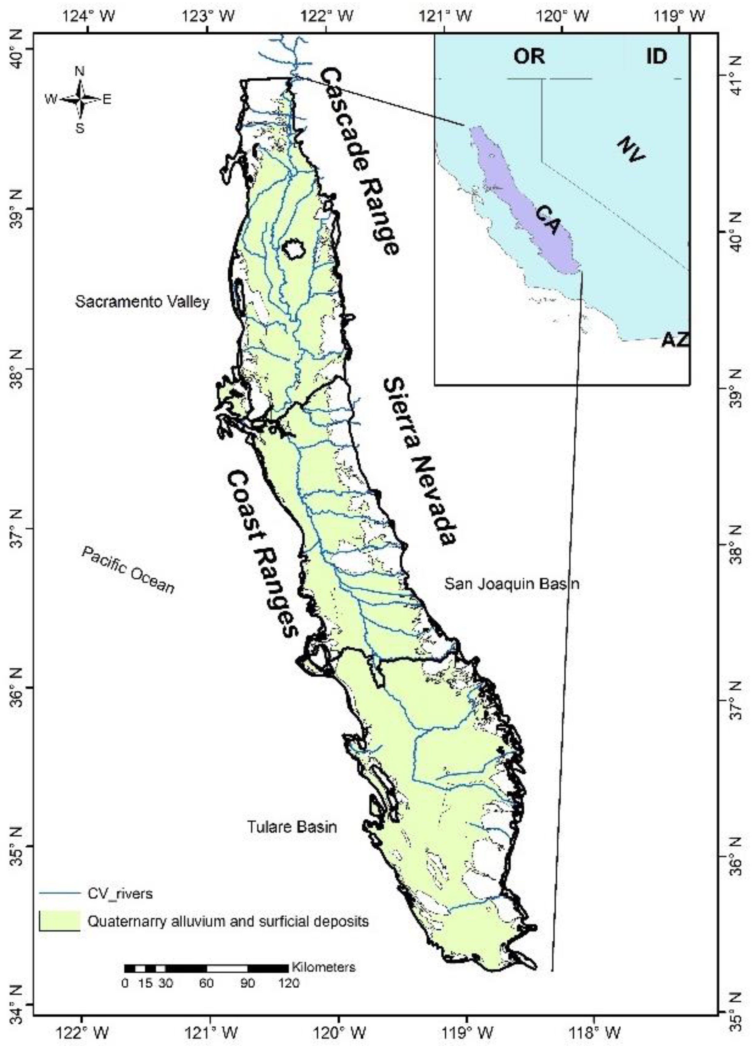
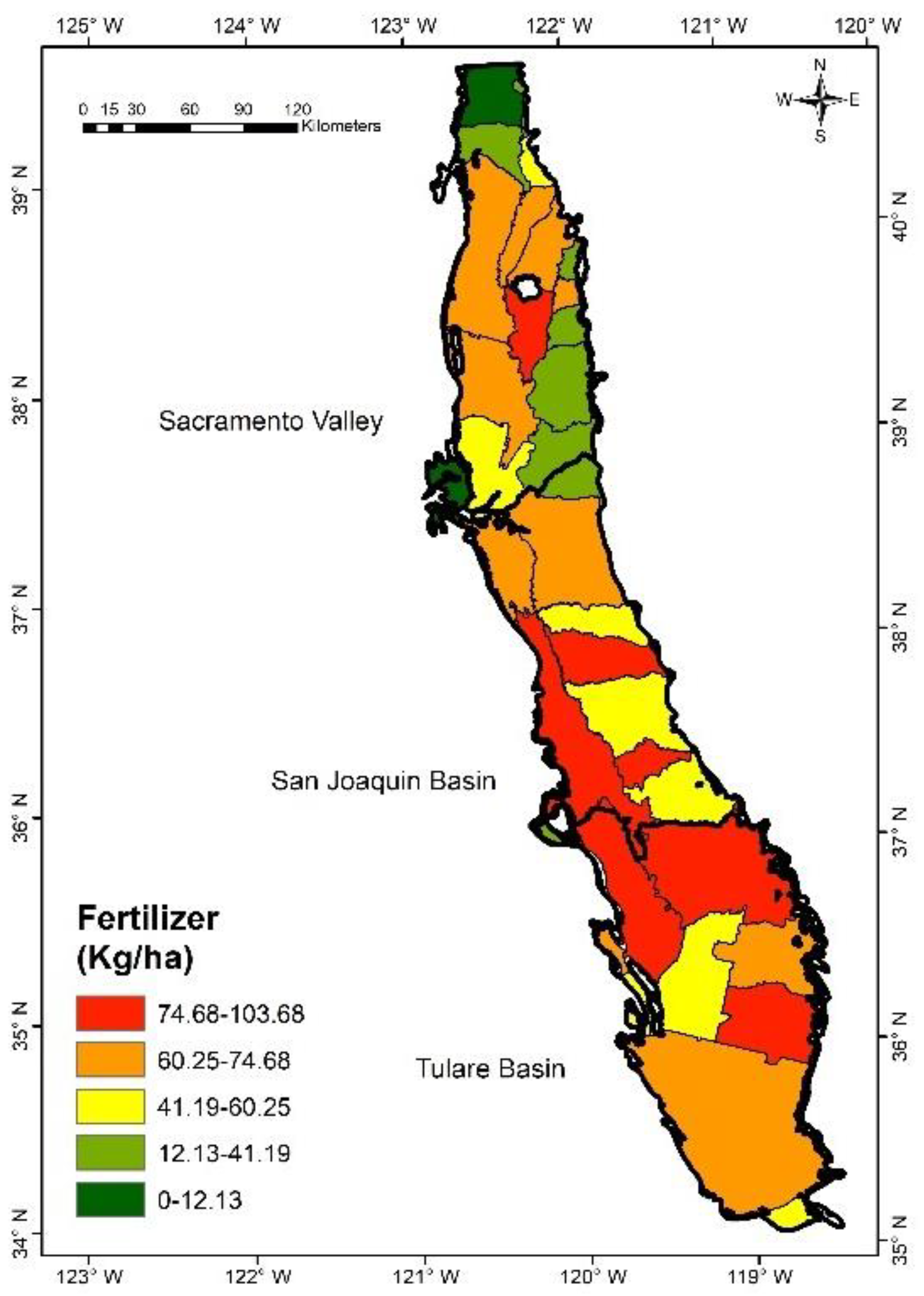
The Central Valley (CV) aquifer lies under one of the most productive areas of the United States. It accounts for 17% of the total national irrigated land used for agriculture and 75% of the irrigated land of the state of California [1]. In the CV, for the past several decades huge amount of chemical nitrogen fertilizer has been applied to increase the crop productivity [2]. Based on a mass balance study, the long-term assessment of nitrogen loading in the Sacramento Valley, San Joaquin Basin, and Tulare Basin of the CV observed significant increase in the nitrogen fertilizer application rate between year 2002–2012 compared to 1991–2001 [3]. The estimated 740,000 tons of nitrogen fertilizer was applied to 6.7 million acres of irrigated farmland in California. The excess nitrogen fertilizer, not absorbed by crops, as a chemical contaminant, easily dissolves in water and leaches into the aquifer to pollute the groundwater [4]. 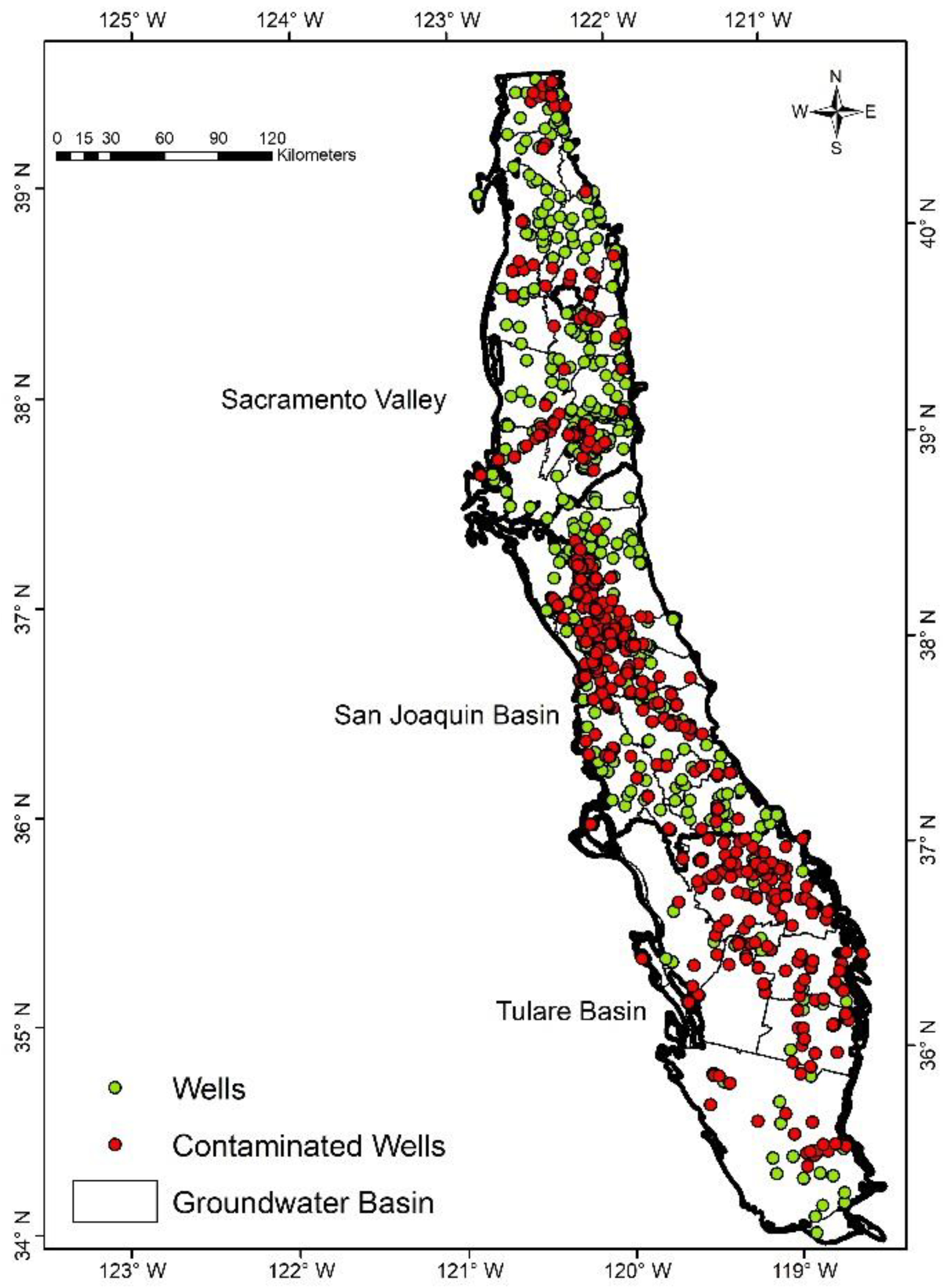Harter [4] estimated more than 80 pounds of nitrogen per acre per year leaching into the groundwater. The nitrate contamination level in some public, domestic, and monitoring wells of the CV have exceeded the EPA maximum contaminant level (MCL) of 10 mg/L [5,6,7]. Several studies have attributed the groundwater nitrate concentration level to agricultural activities of the region [7,8,9].

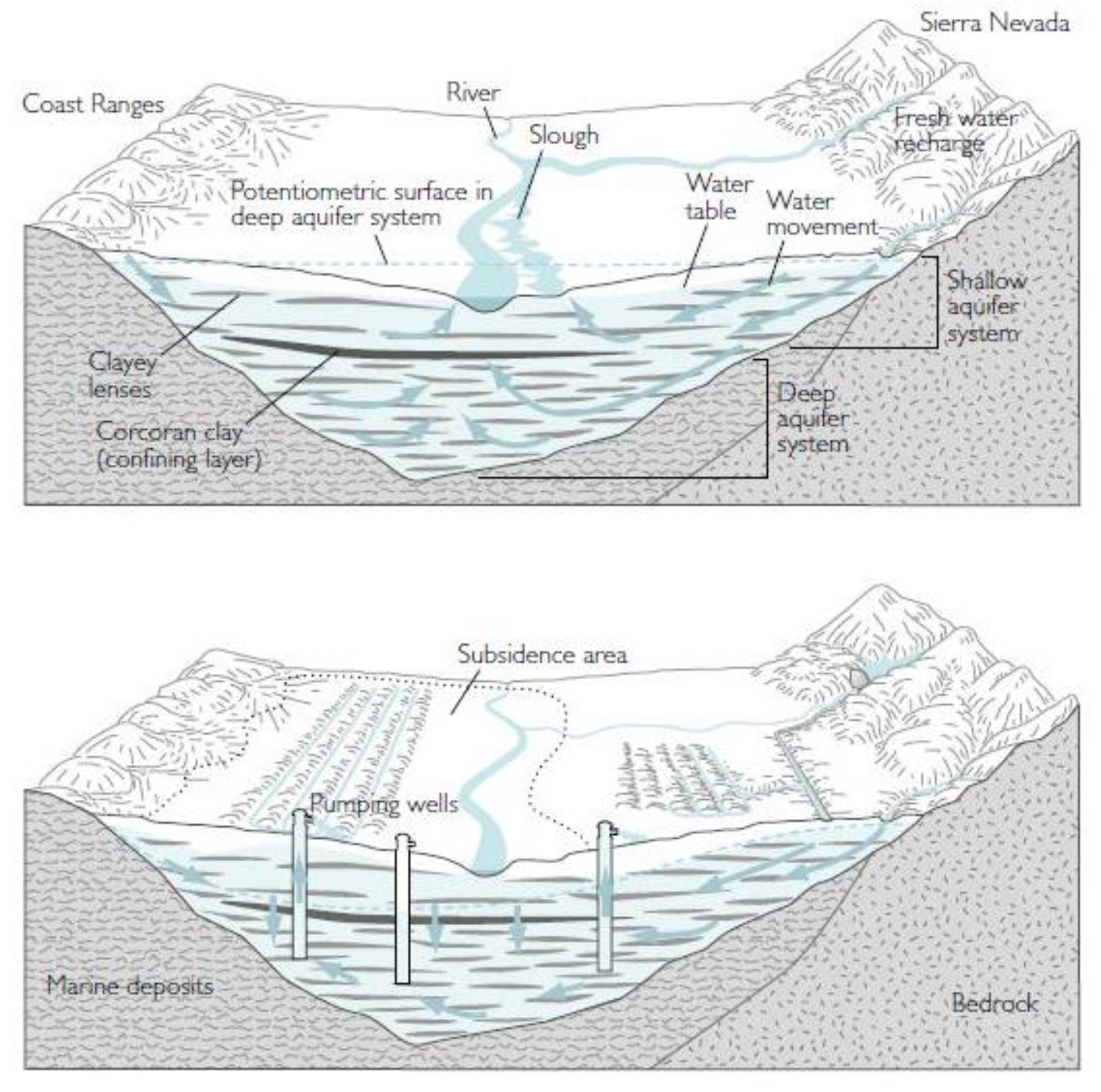
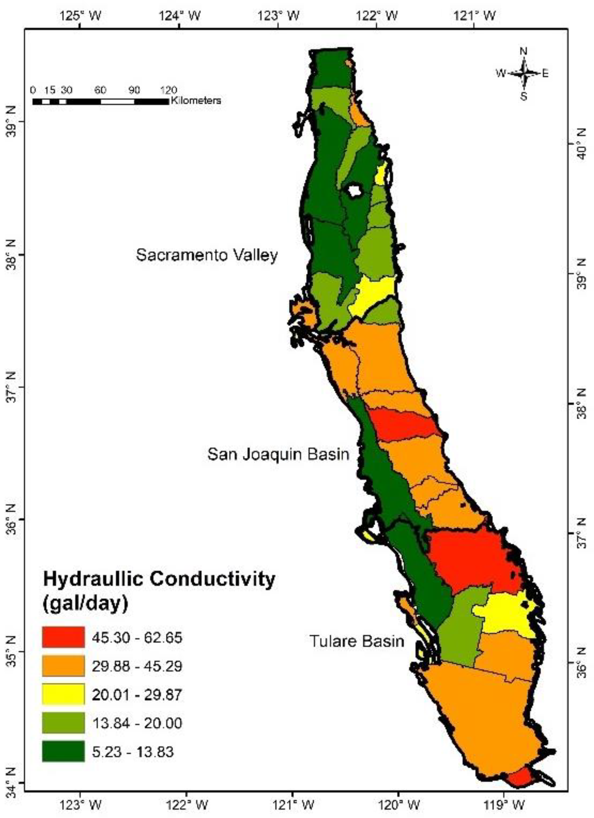
The susceptibility of groundwater nitrate contamination is influenced by the aquifer characteristics and geochemical condition of the valley, which could enhance or reduce the leaching rate of nitrate into the aquifer [10]. The hydrogeological conditions like shallow water table, high permeability, and high hydraulic conductivity enhance the downward percolation rate of the nitrate into the aquifer. The lower nitrate concentration has been found in reducing environment due to denitrification process that breaks down nitrate into nitrogen gas [11]. The interplay of these different environmental factors often makes it difficult to predict the areas vulnerable to groundwater nitrate contamination. However, identification of vulnerable areas is of extreme importance for groundwater management agencies to develop site-specific mitigation tools and adopt appropriate policies to mitigate the contamination.

The process-based, statistical, and index- overlay methods are the most widely used techniques to assess the vulnerability of the aquifer to groundwater nitrate contamination. Process-based methods are deterministic ways of predicting the nitrate contamination based on solute transport model. Physical, chemical, geological, and biological processes are considered to simulate the subsurface flow of contaminants, involving complex numerical computations [12]. The process-based methods are effective at local scale prediction, but because of detailed data requirements, they are not practical for large spatial scale prediction [13,14].

Statistical methods are robust ways of analyzing the relationship between groundwater nitrate contamination and predictor variables. The multiple linear regression calculates individual coefficients of the predictor variables to measure its contribution to the nitrate contamination [15,16]. There are numerous studies where logistic regression has been applied to calculate the probability of nitrate concentration above the background value [17,18]. Other statistical methods have been used to measure the linear trend [19], comparing the mean nitrate concentrations under different agriculture settings [8] or the difference of nitrate concentration over different time intervals [20]. The computing power of statistical method to process large data in a short period of time signifies the strength of these methods. However, careful analysis is still warranted in the interpretation of statistical output. The availability of sufficient data meeting the requirement of the statistical analysis often becomes challenging. Further, site-specific nitrate contamination data or data covering regional or national scale are sparse and not uniform, which could cause biasness in the statistical results. Long term monitoring of groundwater data over large spatial scale demands government priority and budgeting over a long period of time.

The index and overlay method uses geological and hydrogeological setting to assess the vulnerability of the study area to the groundwater contamination. This method is preferred for its simplicity to map the vulnerable areas by using different layers of data that affect the transport of nitrate to create spatially oriented index values. Several index and overlay methods has been applied to assess the vulnerability of aquifer such as DRASTIC [21], GOD [22], AVI, and SINTACS [23]. The selection of correct method is important in generating the vulnerability map and site-specific methods have been proposed in different study. For example, EPIK and RISK methods are used for Karst aquifers, the AVI method for porous aquifers and GOD for sedimentary aquifers. DRASTIC has been a widely used method and is applicable to all aquifer types [21]. DRASTIC was developed by Aller et al. (1987) for the United States Environmental Protection Agency (EPA). The DRASTIC method has been applied frequently to assess the vulnerability of the study area to groundwater nitrate contamination [13,14,24,25,26]. Recently, the application of GIS techniques has enhanced the ability to process different data layers to compute the DRASTIC Index values [27,28]. The method has been relatively successful in generating the vulnerability map with minimum error in the model results. It is important to understand that the selection of vulnerability method could produce difference in the output map and therefore researcher should be aware in using the correct method.

Some of the limitations of DRASTIC method include its subjectivity in assigning the weight values to its variables and the dimensionless index values [29,30]. The pre-assigned weights to DRASTIC variables could be inaccurate for a given study area and could create biases in the calculation of DRASTIC Index values, as the influence of variables to vulnerability could change in different study areas. The generalization of the subjective weights of DRASTIC method have been criticized in several studies [30]. The need to add additional variables to increase the efficiency of method has been realized in many studies. Several studies have modified the DRASTIC variables by adding landuse variables [14,31] and calibrating the point rating of variables based on correlation of nitrate concentration and hydrological variables to the model or modified the rating values to increase the efficiency of the method [32]. Some authors have also emphasized on the availability and reliability of data suitable for the DRASTIC methods and interdependence of variable in linear combination could cause uncertainty in the method [30].

Index–overlay methods, process-based methods, and statistical methods all have their strengths and limitations. The pros and cons of these methods can be accounted to correctly meet the scientific objective, budgeting constraints, and to aid in the decision supporting process. In this study, we developed two nitrate vulnerability maps: one based on the optimized-DRASTIC method and the other based on the new Geodetector-Frequency Ratio (GFR) method proposed here. Geodetector is a relatively new method that measures the correspondence between the incidence rate of events and the spatially stratified heterogeneity of explanatory variables [33]. The Geodetector calculates the Power of Determinant (PD) values for each contributing factor (or independent variable) based on the spatial variance analysis, which estimates the degree of influence a variable has on the incidence rate, which is groundwater nitrate contamination in this case. The Frequency-ratio (FR) is a technique commonly used in landslide susceptibility mapping [34,35] and was recently introduced in groundwater vulnerability mapping [36]. The FR measures the percent of area with incidence in each interval of a factor to the percent of area of that interval relative to the whole study area. The interval with higher FR is more susceptible to the incidence. We assigned the weights to the predictor variables based on the Geodetector results and assigned the rating based on the FR method to compute the Nitrate Susceptibility Index (NSI) using the geometric mean [37].

Therefore, the objective of this paper is to generate a nitrate vulnerability map of the CV using the quantitatively derived rating and weights of the variables using GFR method and to compare the result with that generated from optimized-DRASTIC model. As will become evident later, the GFR method generated a map that is more consistent with the spatial distribution of contaminated wells in the CV, because GFR method integrates Geodetector and Frequency-Ratio method, which overcomes the subjective assignment of weights and rating values of variables in optimized-DRASTIC method.

2. Methods

2.1. Central Valley Aquifer System

The Central Valley (CV) is one of the largest structural troughs in California (CA) that is predominantly covered with continental and marine sediments. The northern one-third of the valley is Sacramento Valley drained by Sacramento River. The southern two-thirds of the valley is San Joaquin valley further divided into San Joaquin Basin and Tulare Basin drained by San Joaquin River. The CV is bounded by Cascade Range and Sierra Nevada in the east and by Coast Ranges in the west (Figure 1).

The valley floor is mostly layered with alluvial deposits and flood plain deposits of river systems. The sediment deposits are predominantly sand and gravel with significant amount of fine- grained silt and clay. The CV is believed to be a single heterogeneous aquifer system [38]. The groundwater flow system in the CV has been altered due to intensive groundwater pumping, causing the water table to drop hundreds of feet thereby increasing hydraulic gradient and directing the groundwater flow into the deeper confined aquifer. Figure 2 shows the change in the flow direction of groundwater before and after the development in the valley. More than 400 feet of water level decline has been measured in the San Joaquin valley. The wells in the San Joaquin are deeper than wells in the Sacramento Valley. The over-pumping of groundwater has induced land subsidence and groundwater quality problem in the CV. The changing hydrogeologic conditions and excess nitrogen fertilizer have complicated the fate and transport of contaminant in the valley [39].

2.2. Nitrate Contamination in the CV at Groundwater Basin Scale

The Central Valley groundwater basin data was downloaded from California Department of Water Resources (DWR) [41] . The groundwater basins were identified by California Department of Water Resources (DWR) based on the extraction and recharge of groundwater in those basins to properly manage the sustainable groundwater project in the CV. The Bulletin 118-California’s Groundwater has more details on the groundwater basins [42].

The groundwater nitrate concentration data was downloaded from National Water Quality Assessment Program (NAWQA), National Water Information System (NWIS) and Groundwater Ambient Monitoring Assessment (GAMA) for the period of 2002 to 2014 to compute decadal average of groundwater nitrate contamination in the sampled wells. A total of 2516 well samples were collected, and 1014 well samples have mean concentration level above 5 mg/L. The number of wells that exceeded the mean concentration level of 5 mg/L were identified in each groundwater basin.

The background concentration of nitrate in groundwater is usually low in the range of 1–2 mg/L and concentration level greater than this is attributed to the anthropogenic sources [43]. The EPA MCL of nitrate in drinking water is 10 mg/L and concentration higher than MCL could cause several health impacts [44]. Therefore, 5 mg/L was selected as the threshold as it is deemed to better capture the spatial variability of nitrate contamination [19]. The total number of well samples and well samples above 5 mg/L in the groundwater basin of the CV is shown in the Figure 3.

2.3. Optimized-DRASTIC Method

DRASTIC is a widely used method for assessing the susceptibility of aquifer to groundwater contamination. The DRASTIC consists of seven different variables which are used as the influencing factors to derive the groundwater susceptibility to contamination. The seven variables are: Depth to water (D), Rate of recharge (R), Aquifer media (A), Soil media (S), Topography (T), Impact of vadose zone (I), and Hydraulic conductivity (C).

Each variable is assigned a subjective weight to indicate its influence on the susceptibility. The source of data for all the DRASTIC variable is shown in

Table 1. Optimized-DRASTIC variable sources.

Variables	Data Source	Processing Summary	Units
Depth to water (D)	California Department of Water Resources [41]	Interpolation using Kriging method.	Feet (ft)
Net Recharge (R)	USGS Mean Annual Natural Groundwater Recharge [46]	Zonal statistics calculated for groundwater basin using raster data.	Inches (in)
Aquifer Media (A)	Surficial Geology of Southwest Principal Aquifer [47]	Classified based on Anning et al. [10]	Categorical Variable
Soil Media (S)	USGS-NRCS data. Soil Hydrologic group [48]	Weighted average of soil hydrologic group calculated for each groundwater basin.	Categorical Variable
Topography (T)	USGS Elevation Derivatives for National Application [49]	Zonal statistics for each groundwater basin.	Percent Slope
Impact of Vadose Zone (I)	California Department of Water Resources Unites States Geological Survey [41,50]	Processed Depth to water table and Permeability data based on Piscopo [51]	Categorical Variable
Hydraulic Conductivity (C)	USGS [50]	Weighted average in each groundwater basin	Gallons per day/ft2

. Here, we adopted an optimized-DRASTIC method, where each variable was classified into five different intervals using the natural breaks classification to capture the local hydrogeological setting of the CV [14,25,32,45]. The higher rating value was assigned if the interval facilitates the vulnerability. The DRASTIC Index (DI) is the linear combination of all the product of variable weight value and rating value of a given interval (see Equation (1)) and an example is shown in

Table 2. Ratings and weights given to DRASTIC variables.

Depth to Water (D)		Recharge Rate (R)
Range	Rating	Range	Rating
10.28–35.9	10	4.82–7.02	1
35.9–66.36	9	7.02–9.03	3
66.36–118.9	7	9.03–17.23	6
118.9–191.43	5	17.23–31	8
191.43–444.34	3	31–107.67	9
Aquifer media (A)		Soil media (S)
Range	Rating	Range	Rating
Quaternary Alluvium	8	Soil hydro group A (Sandy, loamy sand, sandy loam)	6
Sedimentary Dominated formation of all ages	6	Soil hydro group B (silt loam, loam)	5
Metamorphic or Igneous units	3	Soil hydro group C (Sandy-clay-loam)	4
		Soil hydro group D (clay loam, silty-clay-loam, sandy clay, silty-clay, clay)	3
Topography (T)		Impact of vadose zone (I)
Range	Rating	Range	Rating
0.11–0.45	10	8–10	10
0.45–0.78	9	6–8	8
0.78–1.32	5	4–6	5
1.32–2.83	3	3–4	3
2.83–10.3	1	2–3	1
Hydraulic Conductivity (C)
Range	Rating
5.23–13.82	1
13.82–19.99	2
19.99–29.87	4
29.87–45.25	6
45.25–62.64	8

.

$$DI=D_r·D_w+R_r·R_w+A_r·A_w+S_r·S_w+T_r·T_w+I_r·I_w+C_r·C_w$$

(1)

where subscript r represents rate and subscript w represents weight.

The computed optimized-DRASTIC Index was then used as a relative evaluation index to describe the susceptibility of the given area to groundwater contamination. High values of Drastic Index (DI) represent the more vulnerable areas and low values represent the less vulnerable areas. The assumptions of DRASTIC methods are: The contaminant is introduced at the ground surface; the contaminant is flushed into the ground by precipitation; the contaminant has the mobility of water; the area evaluated is 100 acres or larger [21].

2.3.1. Development of Optimized-DRASTIC Variables

The seven DRASTIC variables were downloaded and processed to calculate the DRASTIC Index. Table 2 shows the weights and rating values assigned to each variables and interval range.

• Depth to Water

Depth to water (DTW) represents the depth to groundwater table below the ground surface. The areas with shallow DTW are considered more vulnerable as it takes less time for contaminant to move into the aquifer in these areas. The data was downloaded from California Department of Water Resources: Groundwater Information Center Interactive Map Application for the year 2014 to represent the end period of the nitrate sampling period from 2002 to 2014 [41]. The data was then interpolated using Kriging method in ArcGIS over the CV aquifer. Kriging has been found effective in the interpolation of depth to water table in many studies [52,53]. Kriging estimates the values at unknown locations using the weighted average of the known values. The weights in the Kriging method are based on the both distance and overall spatial arrangement of the well samples which is calculated using the variogram technique. A function that best fits the measured data is used to predict the value at the unknown location. The ordinary kriging was selected with minimum standard error. The mean zonal statistics was calculated for each groundwater basin using the interpolated DTW value.

• Recharge Rate

The recharge rate is the rate at which water on the land surface percolates into the aquifer. The percolation rate of water into the aquifer depends on the characteristics of vadose zone. Recharge rate is higher in permeable areas with large fractures in rocks or in unconsolidated sand and gravels, where water can easily pass through the interspace between the soil or sand particles. Soil layer that consists of higher percent of clay reduces the travel time of groundwater into the aquifer and thus the recharge rate. Recharge rate also tends to be higher in high altitude where precipitation is higher, increasing the chances of more water percolating into the groundwater [1].

The data for estimated mean annual natural groundwater-recharge in the Conterminous United States was downloaded from United States Geological Survey (USGS), which is a raster dataset with 1 km resolution [46]. The zonal mean for each groundwater basin was calculated using the raster data and classified into five intervals of natural breaks and assigned corresponding ratings for optimized-DRASTIC method.

• Aquifer Media

The aquifer media is the underlying geology that determines the water holding capacity of rock materials. Groundwater is stored in the pores and fractures of rocks within the aquifer which determines the groundwater flow rate. Karst limestone, basalt, and unconsolidated sand and gravel have higher flow rate due to their structure than metamorphic, igneous rock, or shales.

The GIS database of geologic units in California is available in the California Geological Survey website [54]. The geologic database identifies the major rock type with unique geocode. These rocks, based on the unique geocode, were classified as Quaternary Alluvium, Sedimentary, Metamorphic, or igneous based on Anning et al. [10]. The corresponding rating values were assigned based on Aller’s et al. [21].

Table 3. Classification and rating values of geologic units.

Geocode	Substrate	Rating
Q, QPc, Qs, Qls	Quaternary Alluvium	8
Mc, M, Ku, J, K, KJf, P, M, E, KI, Mc, Tc, KI, J, Tc, E, Ec, Ep, O, P, Qoa	Sedimentary Dominated formation of all ages	6
gb, grMz, Tv, TvP, Mzv, um, grMz, gb, mv, m, Qvp, gr-m, m, um	Metamorphic or Igneous unit	3

shows the geocode classification system and rating values.

• Soil Media

Soils are grouped based upon their composition and runoff potential and can be represented by soil hydrologic group. The soil hydrologic group data was extracted from soil data for Conterminous United States derived from the Natural Resource Conservation Service (NRCS) State Soil Geographic (STATSGO) data base.

Soil hydrologic group was numerically assigned based on the Battaglin’s methods. The codes were 1, 2, and 3 for hydro groups A, B, and C, respectively. The number 4 was assigned to hydro group A/D, B/D, and C/D [48]. The map unit identifiers (MUID) in the dataset represent the unique hydrologic conditions. Each unique MUID hydrologic condition was intersected with the groundwater basins. The percent of area of each MUID in each groundwater basin was multiplied by the soil hydrologic value. The product of each proportional area and MUID values was then added up to represent the total value hydrologic value of each basin. The values ranged from 1 (well drained-A) to 4 (poorly drained-D) to represent the soil media of the CV.

• Topography

Topography in DRASTIC is the slope of land surface. The steep topography has less chance of infiltration due to runoff. The plain areas will have higher infiltration rate and hence increase the chance of infiltration of nitrate into the aquifer. The slope data was downloaded from USGS (Elevation derivatives for National Application (EDNA), 2005) [49], which was derived from the National Elevation Dataset (NED). Mean zonal statistics of slope value were calculated for each groundwater basin and classified based on natural breaks classification.

• Impact of Vadose Zone

The vadose zone is the layer above the water table and the Impact of vadose zone is critical to the movement of groundwater into the aquifer. The texture of this layer controls the attenuation capacity of the contaminants including biodegradation, naturalization, mechanical filtration, chemical reaction, volatilization, and flow rate of groundwater [21]. The longer residence time of groundwater in vadose zone provides longer time for the attenuation. The Impact of Vadose Zone value was calculated using the soil permeability and depth to water table values, based on the method described in reference [51]. The vadose zone values were then given rating values to calculate in the optimized-DRASTIC method.

• Hydraulic Conductivity

Hydraulic Conductivity measures the easiness of water flowing into the aquifer. It depends on the soil pore geometry, the fluid viscosity, and density. The higher hydraulic conductivity increases the water percolation rate into the aquifer. Area and depth weighed average hydraulic conductivity values is available in the USGS website [50]. The weighted hydraulic conductivity values for each groundwater basin in the CV were calculated by adding the proportional MUID area and hydraulic conductivity values within each basin.

2.4. Geodetector-Based Frequency Ratio Method (GFR)

2.4.1. Geodetector Method

The Geodetector-based frequency ratio method (GFR) integrates the Geodetector method and Frequency Ratio method to calculate Nitrate Susceptibility Index (NSI). The Geodetector method is a spatial variance technique, which measures the spatial association between the predictor variables and the dependent variable [55]. The assumption is that if a predictor variable leads to groundwater nitrate contamination, the contamination would exhibit a spatial distribution similar to that of the predictor variable [55,56]. The Power of Determinant (PD) value for each predictor variable was obtained by calculating the ratio of sum of variances of predictor variables in the stratified zones (stratified heterogeneity) to the total variance in the entire study area. It is given by the formula:

$$Power of Determinant \left(PD\right)=1-\frac{1}{N{\sigma }^2}{\displaystyle \sum }_{i=1}^L{N}_i{\sigma }_i^2,$$

(2)

where N is the total sample in the entire study area; L is the number of zones of predictor variable; $\sigma$ is the variance; and subscript i represents the i-th zone.

If the spatial associate is real, the local variances should be close to zero or very small. If the spatial associate is not there, then the local variance is expected to be the same as the global variance. So, the spatial association can be measured by comparing the local and global variances and encapsulated in the Power of Determinant (PD), which is calculated as 1 minus the ratio of local to global variances. The PD value ranges between 0 and 1, with 1 meaning perfect spatial association and 0 no association. The significant variables at significance level of 0.05 were retained to calculate relative PD values of each variables. Details on the processing of Geodetector method can be found in reference [26]. The PD values of significant predictor variables were normalized to calculate its relative contribution in relation to other significant variables. It is given by the formula below:

$$Relative PD=\frac{PD value of Predictor variable}{Sum of PD values of all significant Predictor variables.}$$

(3)

2.4.2. Development of Geodetector Variables

The Geodetector method was performed on 12 different predictor variables, which comprised of source variables, aquifer susceptibility variables, and geochemical condition of the CV that could alter the groundwater nitrate contamination of the CV. The details on the processing of the variables can be found in reference [26].

Table 4. Explanatory variables in Geodetector method.

Explanatory Variables	Data Source
Farm Fertilizer (kg/ha)	United States Geological Survey (USGS) [57]
Manure (kg/ha)	United States Geological Survey (USGS) [58]
Cropland (%)	National Landcover database (NLCD) [59]
Permeability (in/h)	STATSGO Soil Characteristics for the Conterminous United States [60]
Precipitation (mm)	PRISM Climate Data based long term historical record from 1981 to 2010 [61]
Slope (%)	Elevation derivatives for national applications (EDNA) [62]
Elevation (m)	National Elevation Dataset (NED) [49]
Clay (%)	United States Geological Survey (USGS)Error! Hyperlink reference not valid [63]
Recharge Rate (mm/Year)	United States Geological Survey (USGS). Error! Hyperlink reference not valid [46]
Dissolved Oxygen (mg/L)	NAWQA and NWIS [64,65]
Iron and Manganese (mg/L)	NAWQA and NWIS [64,65]

below shows the summary of the data sources of the predictor variables. All of these variables were input into the Geodetector software to calculate their PD values and significance level. The software is available for free at http://www. geodetector.org.

2.4.3. Frequency Ratio Method

The Frequency Ratio (FR) method was used to obtain the rating values on different intervals of significant predictor variables. Each numerical predictor variable is discretized into different intervals to represent the stratified heterogeneity. Since we used groundwater basin as our basic unit, the number of wells within each interval was counted and divided by total number of wells of the study area to obtain percent of wells in each interval. Similarly, the number of contaminated wells in each interval was counted and divided by total number of contaminated wells of the study area to obtain percent of contaminated wells in each interval. Frequency ratio is the ratio of the two percentages as follows:

$$Frequency Ratio=\frac{Percent of contaminated wells in each interval }{Percent of wells of the related interval}.$$

(4)

Frequency Ratio is a commonly applied technique in landslide studies to calculate the landslide incident rate in vulnerable areas. The Frequency Ratio value of greater than 1 indicates strong relationship with the groundwater nitrate contamination and less than 1 indicates weak relationship [66].

2.4.4. Geodetector Frequency Ratio Index

The Geodetector Frequency- Ratio Index was calculated as a weighted geometric mean [37] using the relative weight of significant predictor variables and their frequency ratio values in each interval given by the formula below:

$$GFR Index={\displaystyle \prod }_{k=1}^n{(A_k)}^{\left(B_k\right)},$$

(5)

where n is the total number of explanatory variables; B_k is the normalized PD values for the kth explanatory variable; and A_k is the frequency ratio of the kth explanatory variable.

3. Results

3.1. Optimized-DRASTIC Method Result

3.1.1. Maps of DRASTIC Variables

Figure 4 shows the distribution of Depth to Water (DTW) in the Central Valley. The DTW was relatively shallow in the Sacramento Valley and deeper in San Joaquin and Tulare Basins.

The hydrogeological characteristics of San Joaquin and Tulare Basins have changed over the years due to excessive pumping of groundwater. This has caused the lowering of water table in this part of the valley [67] .

The Net Recharge rate in the CV is shown in Figure 5. The recharge rate was mostly low in most part of the valley and relatively higher around eastern flank of the valley, mainly around southeastern San Joaquin Basin and northeastern Tulare Basin. The CV lies in the rain shadow due to the presence of Coastal Range in the west acting as orographic barriers to the moisture laden onshore oceanic winds. The eastern part of the valley is Sierra Nevada with higher elevation. This leads to higher annual precipitation rate due to orographic effect and increasing recharge rate there.

Most of the CV is underlain by Quaternary alluvium and surficial marine and non-marine sedimentary rocks deposited from Jurassic to Holocene period (Figure 6). These deposits comprise mostly unconsolidated and semi-unconsolidated sediments, including terrace deposits, sandstone, shale, and gravel deposits. The changes in the deposition environment of the CV has caused overlaying of continental deposits on the marine depositions and formed the freshwater aquifer of the valley [1]. Figure 7 shows the soil media map of the CV aquifer. The Sacramento Valley had mainly soil of hydrologic groups C and D. The San Joaquin and Tulare Basins were mostly hydrologic groups A and B. This soil hydrologic group C was moderately fine to fine textured which permits slow infiltration rate of water through them. Hydrologic soil group A soils drain easily as they have sands or gravels and high infiltration rates. Hydrologic group B soils are mostly moderately fine texture to moderately coarse texture that permits moderately well drained soils.

The CV had mostly low slope areas between slope percent of 0 to 2% (Figure 8). It can be observed from the figure that Tulare basin had more low slope areas than other parts of the valley. The Impact of Vadose Zone (IVZ) is represented in the Figure 9. The San Joaquin Basin had higher IVZ ratings than Sacramento Valley and Tulare Basin. The Hydraulic Conductivity was low around Sacramento Valley compared to San Joaquin and Tulare Basin (Figure 10).

3.1.2. DRASTIC Susceptibility Index

The optimized-DRASTIC Susceptibility Index (DI) for the CV was generated using the method described in the Method section (see Figure 11). The DRASTIC Index ranged from 103 to 193. The DRASTIC scores were separated into five different intervals based on natural breaks classification.

The general pattern of high index values was observed in the eastern side of the valley compared to western side. The Tulare Basin had high index values in the eastern side and low to very low in western side. The San Joaquin Basin had mostly very high to high index values except small percent of area towards the western flank. The Sacramento Valley also showed relatively higher index values in the eastern part than the western part of the valley.

3.2. Geodetector-Based Frequency Ratio (GFR) Method Result

3.2.1. Geodetector Power of Determinant (PD) Values and Normalized PD Values

The power of determinant (PD) values from the Geodetector method is shown in

Table 5. PD values and normalized PD values of significant predictor variables.

Variables	Power of Determinant (PD)	Significance Level	Normalized PD
Precipitation	0.27	<0.05	0.29
Fertilizer	0.21	<0.05	0.23
Elevation	0.18	<0.05	0.20
Manure	0.16	<0.05	0.17
Clay	0.10	<0.05	0.11

below. Shrestha and Luo [26] calculated precipitation, fertilizer, elevation, manure, and clay as the most significant variables in the CV with high PD values out of 12 different explanatory variables. These significant variables suggest the significance of their spatial heterogeneity in contributing to the groundwater contamination in the CV. Here, we normalized the PD values to be used as the relative weights in the GFR method. The normalized PD values of the all the significant variables is also shown in the Table 5 below. The precipitation had the highest relative PD value of 0.29 followed by fertilizer, elevation, manure, and clay.

3.2.2. Geodetector Variables Map

Figure 12, Figure 13, Figure 14, Figure 15 and Figure 16 show the five statistically significant variables used in the GFR method. All variables were discretized into five zones according to the natural breaks method [68]. The precipitation map (Figure 12) of the CV shows low precipitation in Tulare Basin and gradually increasing towards the San Joaquin Basin, and highest around the Sacramento Valley. Figure 13 shows the fertilizer loading in the CV aquifer. The fertilizer loading in the CV was very high around Tulare Basin and San Joaquin Basin. Sacramento Valley had only slightly lower fertilizer loading than San Joaquin and Tulare Basin.

The manure loading was higher in San Joaquin Valley and Tulare Basins than that in the Sacramento Valley (Figure 14). The elevation of Sacramento Valley and San Joaquin Basin was slightly lower than that of the Tulare Basin (Figure 15). The percent of clay was higher in Sacramento valley than that in San Joaquin and Tulare Basins (Figure 16). It was lowest around eastern flank of San Joaquin Basin and Tulare Basin.

3.2.3. Frequency Ratio Method

The Frequency Ratio (FR) value in each interval for all the significant predictor variables is shown in the

Table 6. Frequency ratio method of significant explanatory variables.

Factor	Range	Level	No. of wells	% wells	No. of contaminated wells	% contaminated wells	Frequency Ratio (FR)
Precipitation	181.24–40.35	1	157	0.06	89	0.09	1.40
mm	240.35–338.4	2	998	0.40	519	0.52	1.29
	338.4–444.97	3	631	0.26	222	0.22	0.87
	444.97–557.87	4	469	0.19	126	0.13	0.67
	557.87–692.83	5	216	0.09	42	0.04	0.48
Fertilizer	0–12.13	1	74	0.03	13	0.01	0.44
Kg/ha	12.13–41.19	2	261	0.11	34	0.03	0.32
	41.19–60.25	3	514	0.21	206	0.21	1.00
	60.25–74.68	4	798	0.32	329	0.33	1.02
	74.68–103.68	5	825	0.33	416	0.42	1.25
Elevation	11.27–39.16	1	736	0.30	242	0.24	0.81
m	39.16–71.86	2	1142	0.46	479	0.48	1.04
	71.86–116.85	3	467	0.19	235	0.24	1.25
	116.85–237.71	4	126	0.05	41	0.04	0.81
	237.71–1180.33	5	1	0	0	0	0
Manure	0–4.38	1	327	0.13	103	0.10	0.78
Kg/ha	4.38–12.1	2	457	0.18	111	0.11	0.60
	12.1–26.58	3	615	0.25	286	0.29	1.15
	26.58–40.47	4	236	0.10	133	0.13	1.40
	40.47–65.48	5	836	0.34	365	0.37	1.08
Clay	13.31–18.55	1	785	0.32	348	0.35	1.10
(%)	18.55–22.65	2	226	0.09	117	0.12	1.28
	22.65–28.30	3	678	0.27	209	0.21	0.76
	28.30–34.84	4	555	0.22	228	0.23	1.02
	34.84–39.54	5	228	0.09	96	0.10	1.04

. The FR values greater than 1 for all the intervals are highlighted in bold in the table. The FR was greater than 1 in low precipitation levels (1 and 2). The FR was greater than 1 in higher fertilizer levels (3, 4 and 5), in low elevation levels (2 and 3), in high manure levels (3, 4, and 5). The FR value for clay percent was greater than 1 at levels 1, 2, 4, and 5.

3.2.4. Geodetector Frequency Ratio (GFR) Index

The Geodetector Frequency Ratio (GFR) index was calculated using the geometric mean (Equation (5)) and the result is shown in Figure 17. The GFR index ranged from 3.70 to 5.17. The GFR index was categorized into natural breaks classification to observe the index distribution over the valley. The index values were highest around San Joaquin Basin and Tulare Basin compared to Sacramento Valley.

Based on natural breaks classification interval of both optimized-DRASTIC and GFR Index, the GFR method predicted more vulnerable groundwater basins to groundwater nitrate contamination than optimized-DRASTIC method (Figure 11 and Figure 17). The GFR Index had 29.27% of wells in the highest interval range (4.96–5.17) compared to only 12.5% of wells in the highest interval range (164–193) in optimized-DRASTIC Index (

Table 7. Natural Breaks classification of DRASTIC and GFR Index.

	DRASTIC			GFR
Index	DRASTIC Index Range	Number of Basins	% Basin	GFR Index Range	Number of Basins	% Basin
Very High	164–193	5	12.5	4.96–5.17	12	29.27
High	147–163	13	32	4.78–4.95	6	14.63
Moderate	129–146	10	25	4.66–4.77	7	17.07
Low	111–128	9	22.5	4.0–4.65	12	29.27
Very Low	103–110	3	7.5	3.70–3.99	4	9.76

). The histogram of DRASTIC index and GFR index values is plotted to observe their distribution (Figure 18 and Figure 19). The mean value for optimized-DRASTIC Index was 141.87 and that for GFR Index was 4.70. The DRASTIC Index values were positively skewed showing only few groundwater basins in the upper range. The GFR Index values were negatively skewed showing relatively higher number of groundwater basins in the upper range.

3.3. Assessment of Vulnerability Index

The results of optimized-DRASTIC and GFR Index were assessed using the Pearson’s correlation analysis and Geodetector method. The higher Pearson’s correlation coefficient (0.7) between percent of contaminated wells in each basin and the GFR Index suggests that GFR Index was a better predictor of groundwater contamination than the DRASTIC Index (

Table 8. PD values and Pearson’s correlation for DRASTIC and GFR method.

Method	PD Values	Pearson’s Correlation
DRASTIC Index	0.062	−0.17
GFR Index	0.49 **	0.70

** statistically significant at the 0.01 level.

). Also, spatial analysis variance (SVA) based Geodetector method was applied to measure the spatial association or consistency of both indices. The results showed higher PD value for GFR method (0.49) than that for DRASTIC method (0.062), again suggesting that vulnerability map of GFR method captured the spatial variability of contaminated wells of the CV aquifer better than the optimized-DRASTIC Index maps. In addition, the PD value for GFR method was statistically significant whereas that for DRASTIC was not. The results suggest that the GFR index values was more consistent with the spatial distribution pattern of groundwater nitrate contamination at groundwater basins of the CV.

4. Discussions

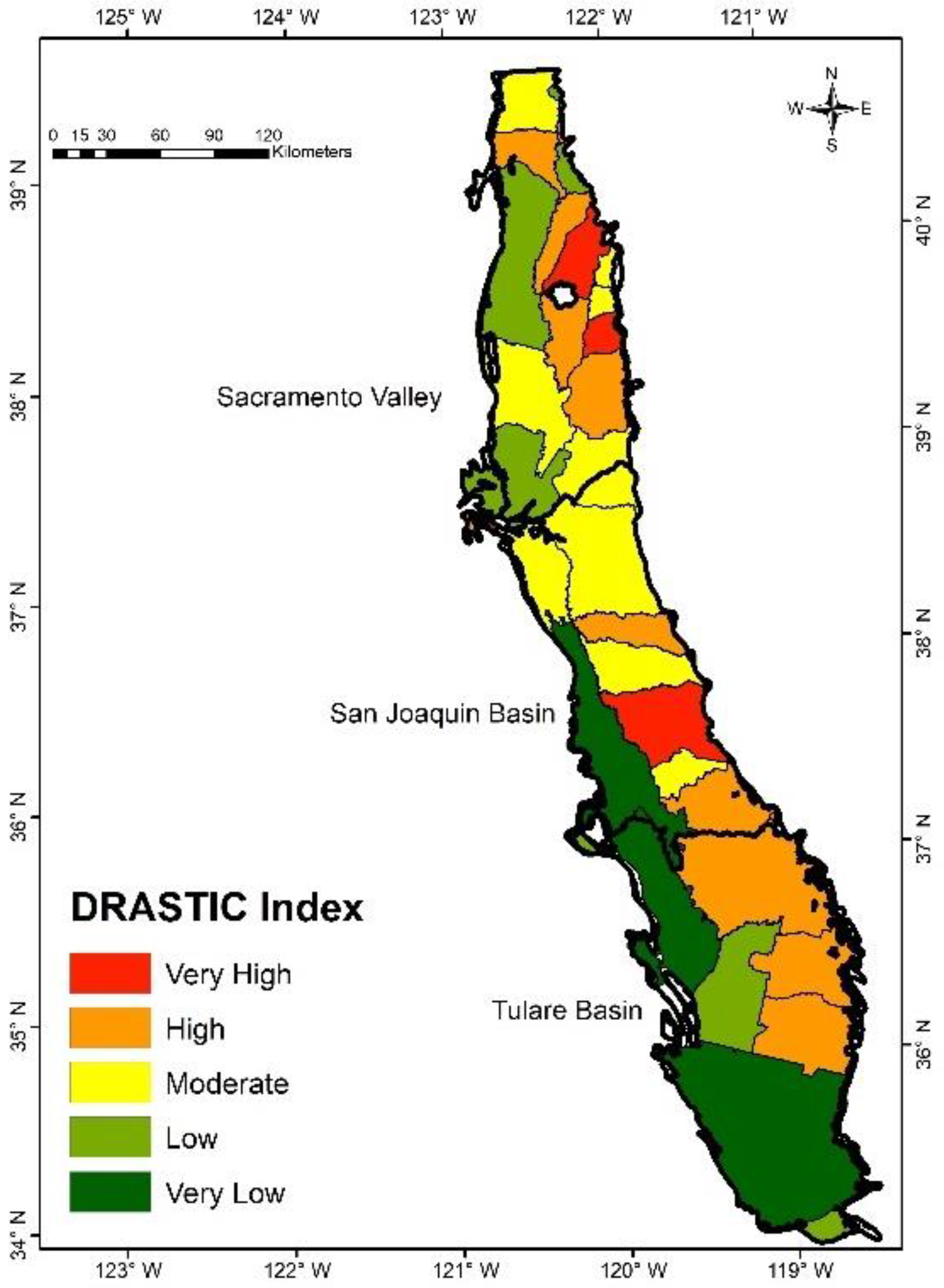
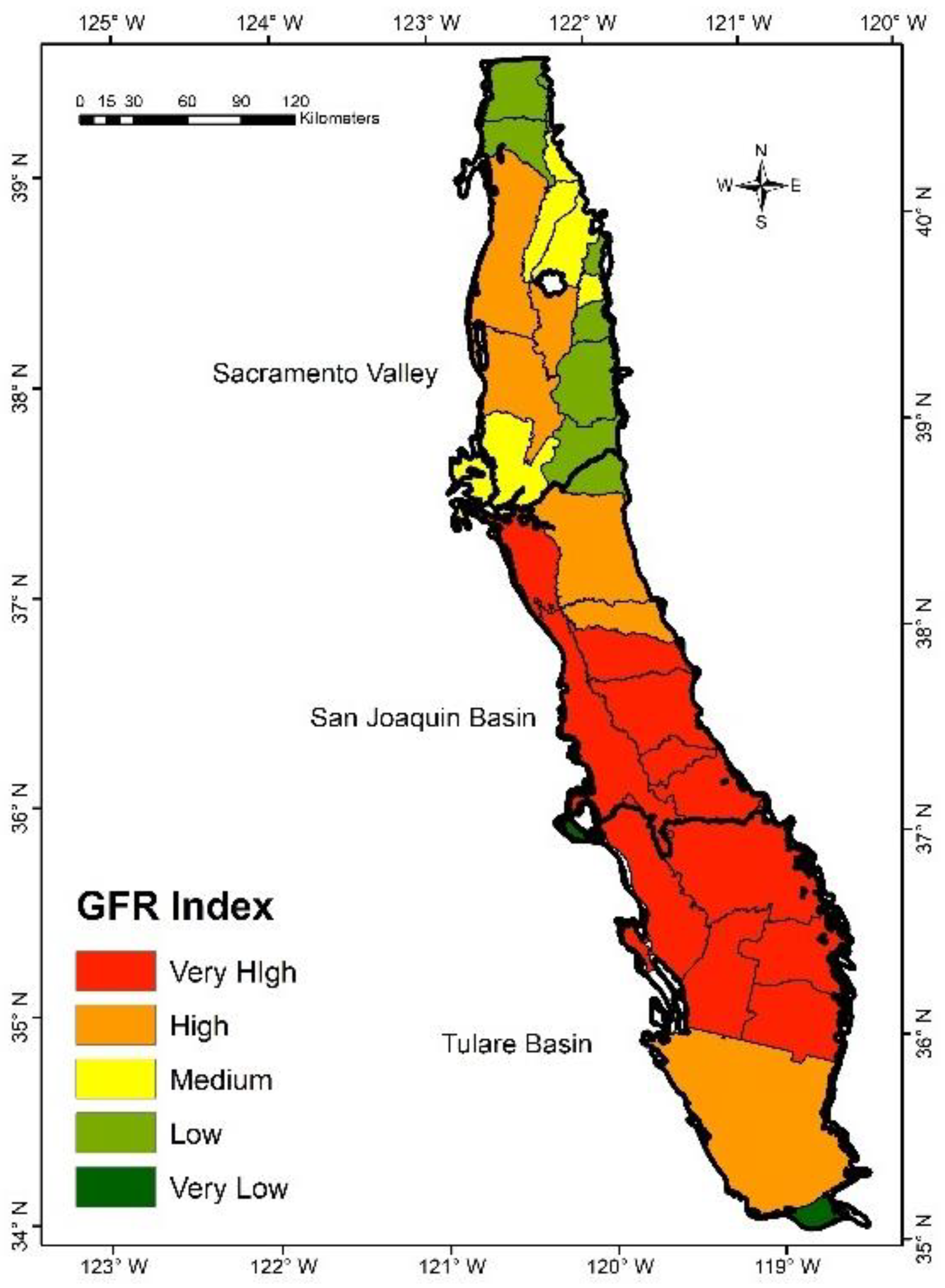
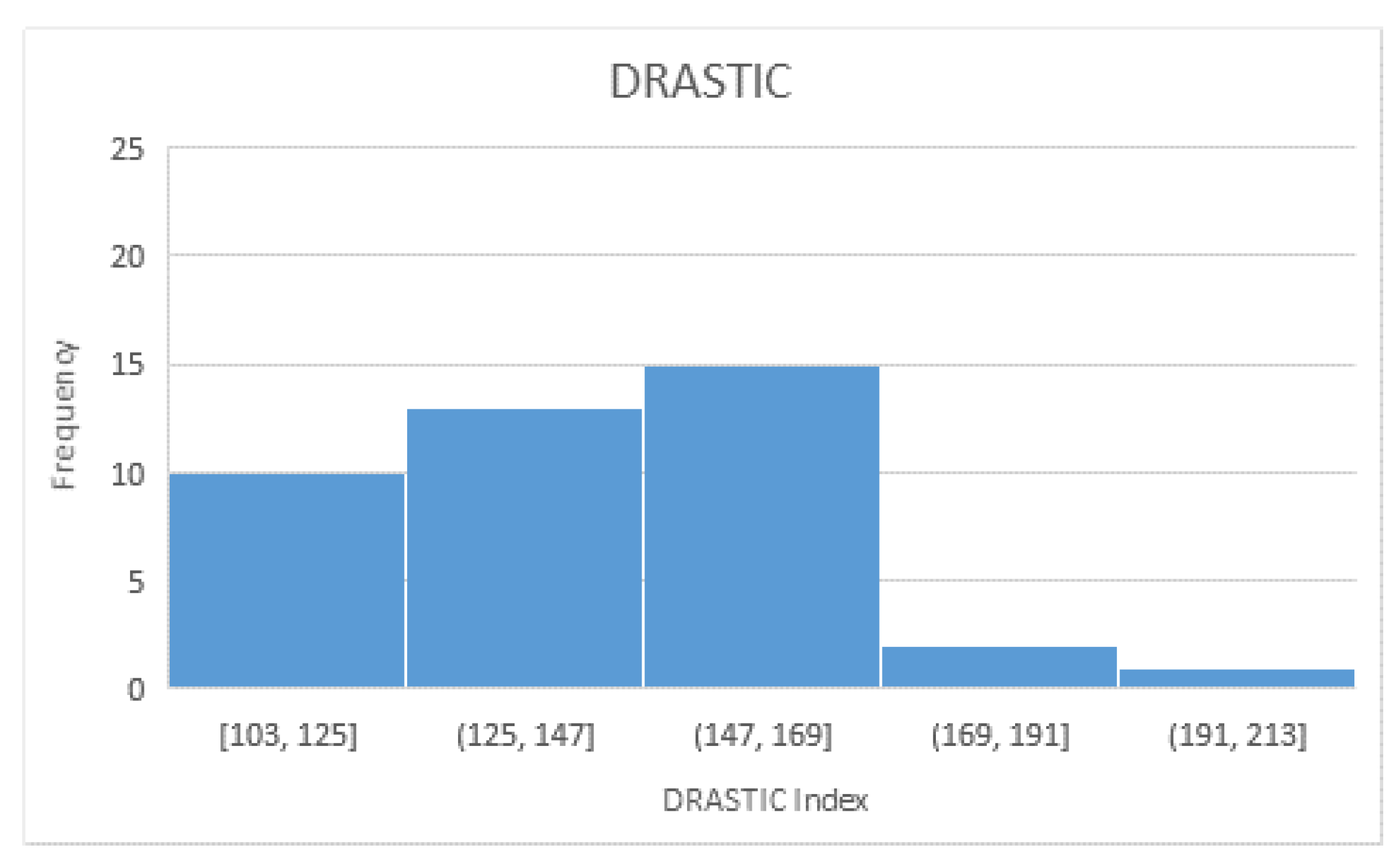
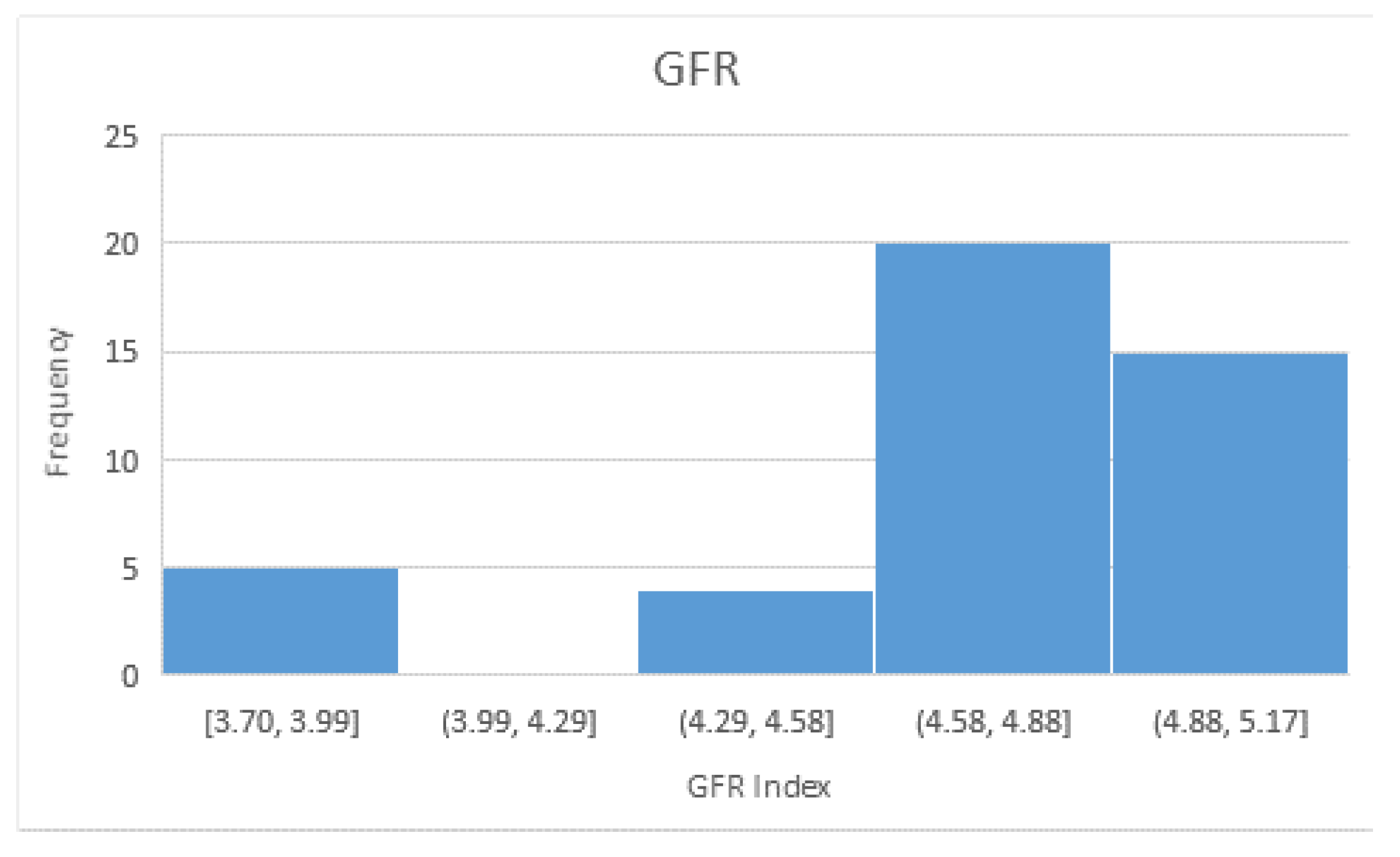
This study developed the new GFR method and applied it to analyze the vulnerability of the Central Valley (CV) aquifer to the groundwater nitrate contamination. The GFR result was also compared with the result derived from optimized-DRASTIC method. The optimized-DRASTIC index values were generally higher in the eastern part of the CV and the GFR method predicted the high vulnerability in the San Joaquin and Tulare basin compared to the Sacramento Valley. The GFR method predicted higher number of basins in the higher index range than the optimized-DRASTIC method.

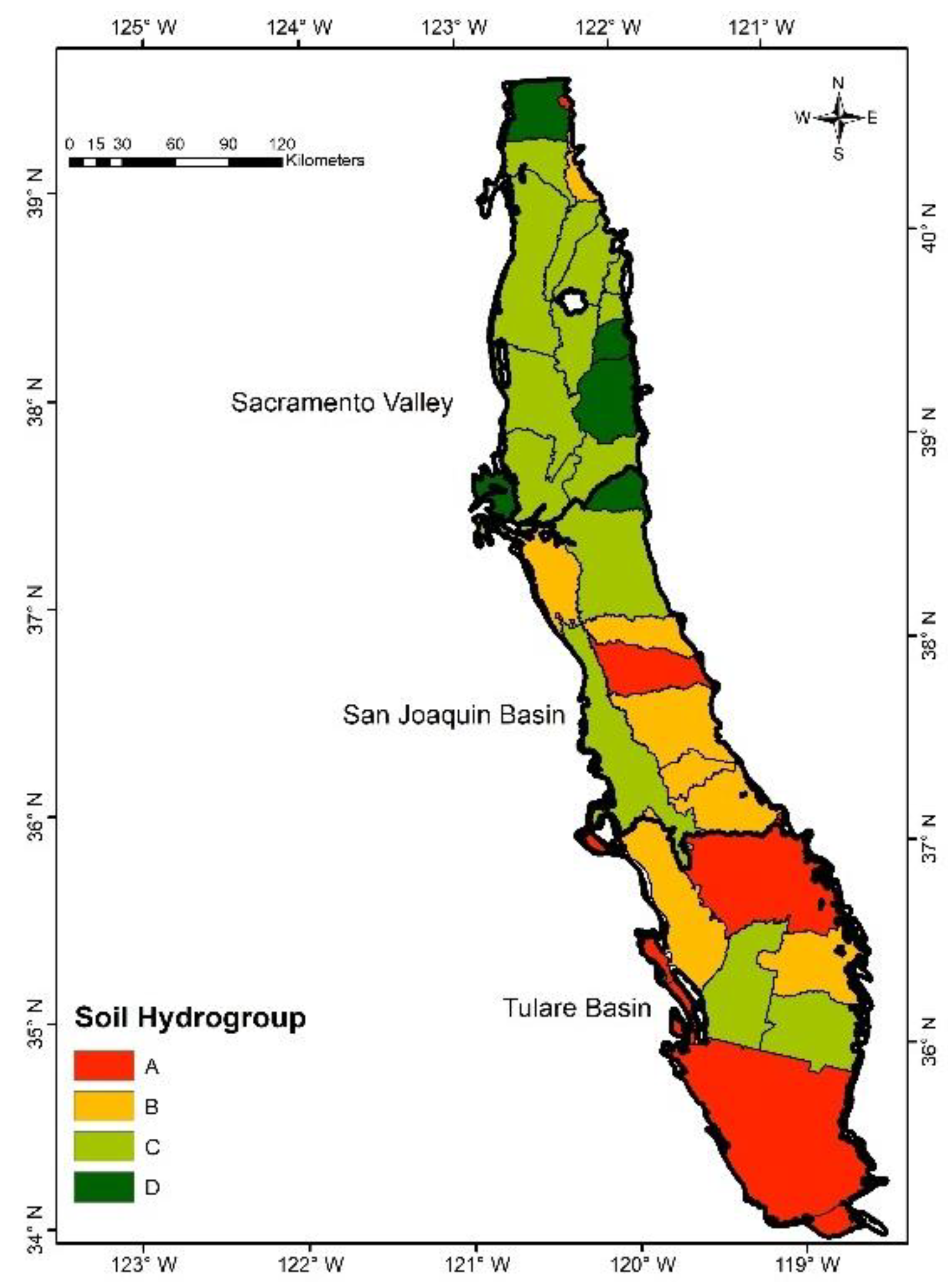
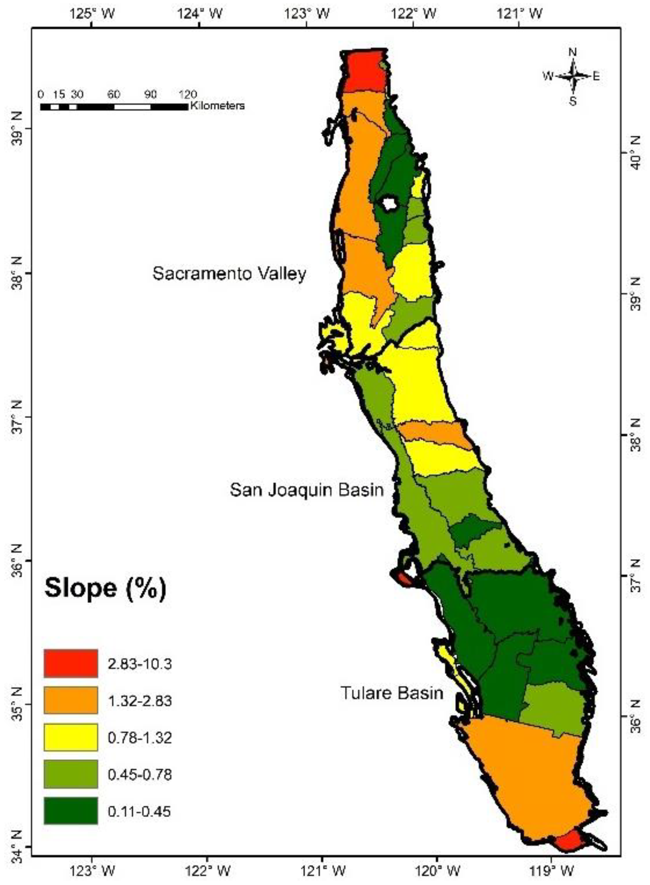
The DRASTIC method is a widely applied groundwater vulnerability assessment method used on local, regional, and national scale. The DRASTIC map can provide a general picture of the vulnerable area of the CV aquifer to the groundwater nitrate contamination. The hydrogeologic variables used in the DRASTIC method are the key variables in determining the susceptibility of the aquifer. The DRASTIC Index values, calculated using weight and rating values of the variables, have been found consistent with other validation techniques in several other studies. In this study, in order to capture the local hydrogeologic condition of the CV, we optimized the DRASTIC method by modifying the range of rating interval of DRASTIC variables using natural breaking classification to calculate the index values [14]. In the GFR method, the incorporation of variables with significant PD values, normalized weight, frequency-ratio, and geometric mean to calculate the GFR Index generated the vulnerability map that was more consistent with the measured groundwater concentration values in the aquifer as measured by both Pearson’s correlation and the PD value of Geodetector method.

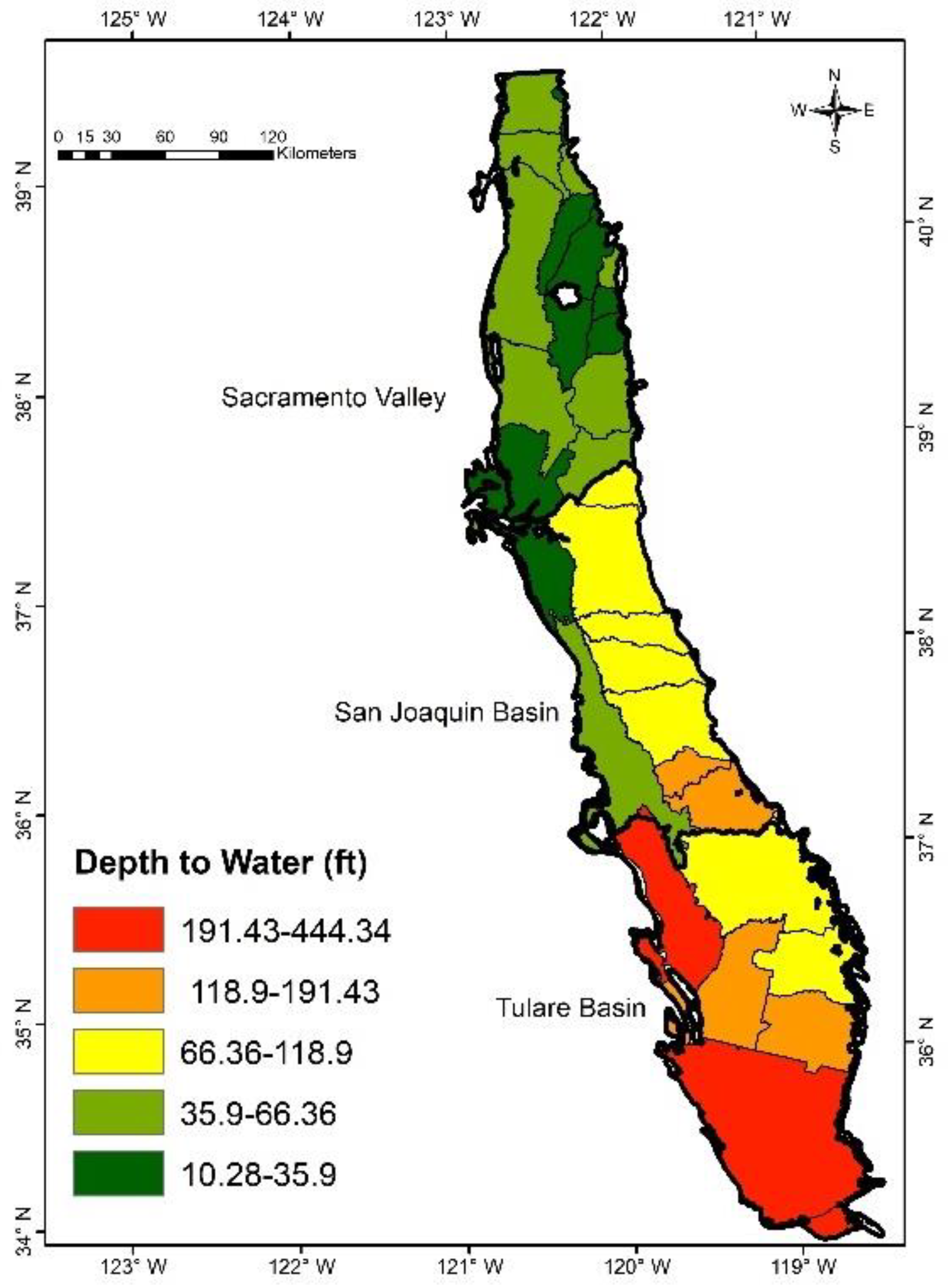
The variables, weights, and rating values in DRASTIC method are preassigned. This pre-assignment of variables, weights, and rating in the DRASTIC method increases the chance of overlooking a variable that might be the underlying factor for increasing the susceptibility of the aquifer. Also, the subjective assignment of weights to the variables may not always correctly represent the influencing variable in a local aquifer. In this study, higher weight is assigned to the Depth to Water (DTW) in the shallow Sacramento Valley than San Joaquin and Tulare basin. However, the hydrogeologic condition of the CV in the southern part of the valley have changed due to hundreds of wells dug to pump the groundwater for irrigation for the last several decades. Although DTW is deep in this part of the valley, the residence time of contaminants is still short due to higher hydraulic gradient caused by heavy pumping, and groundwater generally flows towards the cone of depression [1]. 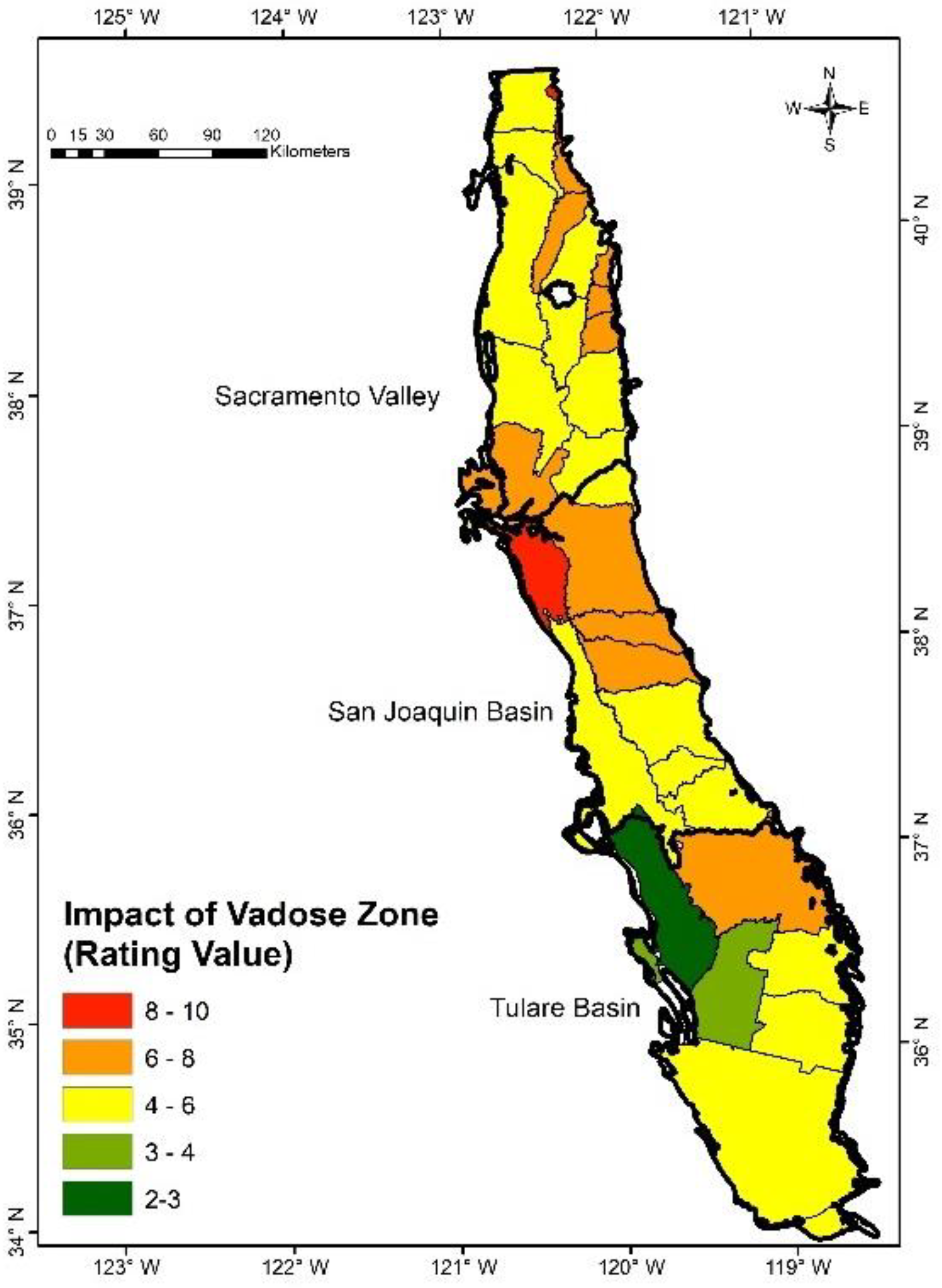The groundwater basins in this part of the CV has the highest priority for groundwater evaluation and monitoring by California Groundwater Elevation Monitoring (CASGEM) [42] .The results of the optimized-DRASTIC method could have been impacted by the inaccurate weighting of DTW. Also, variables specified by DRASTIC method are not always easily available for the study area. In this study, impact of vadose zone (IVZ) data was not easily available for Central Valley. Here, we calculated the IVZ data based on depth to water and permeability [51]. The selection process of site specific data to correctly represent contamination in the data processing is crucial to understand the contaminant’s spatial distribution. The DRASTIC method has been criticized for its lack of ability to include the site-specific variables in the method. Landuse characteristics and other variables have been added to the DRASTIC method to increase its prediction accuracy.

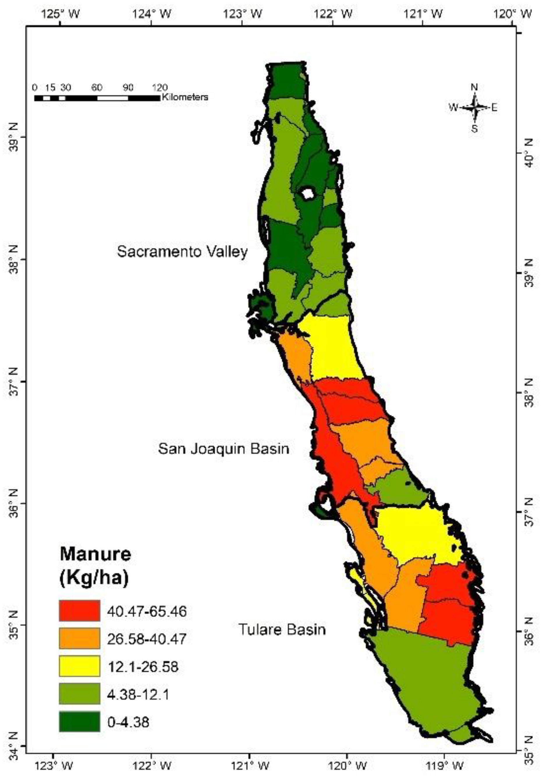
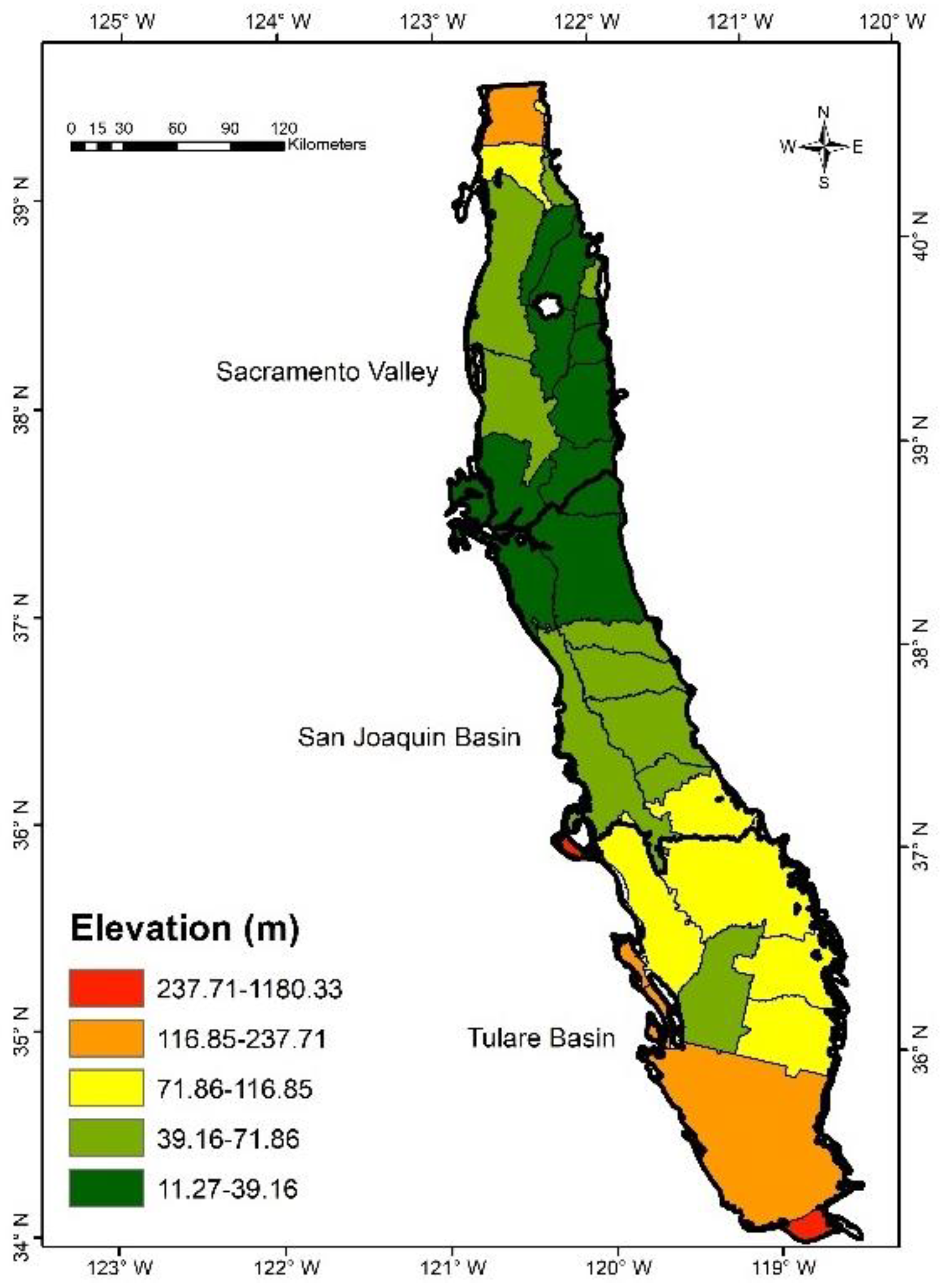
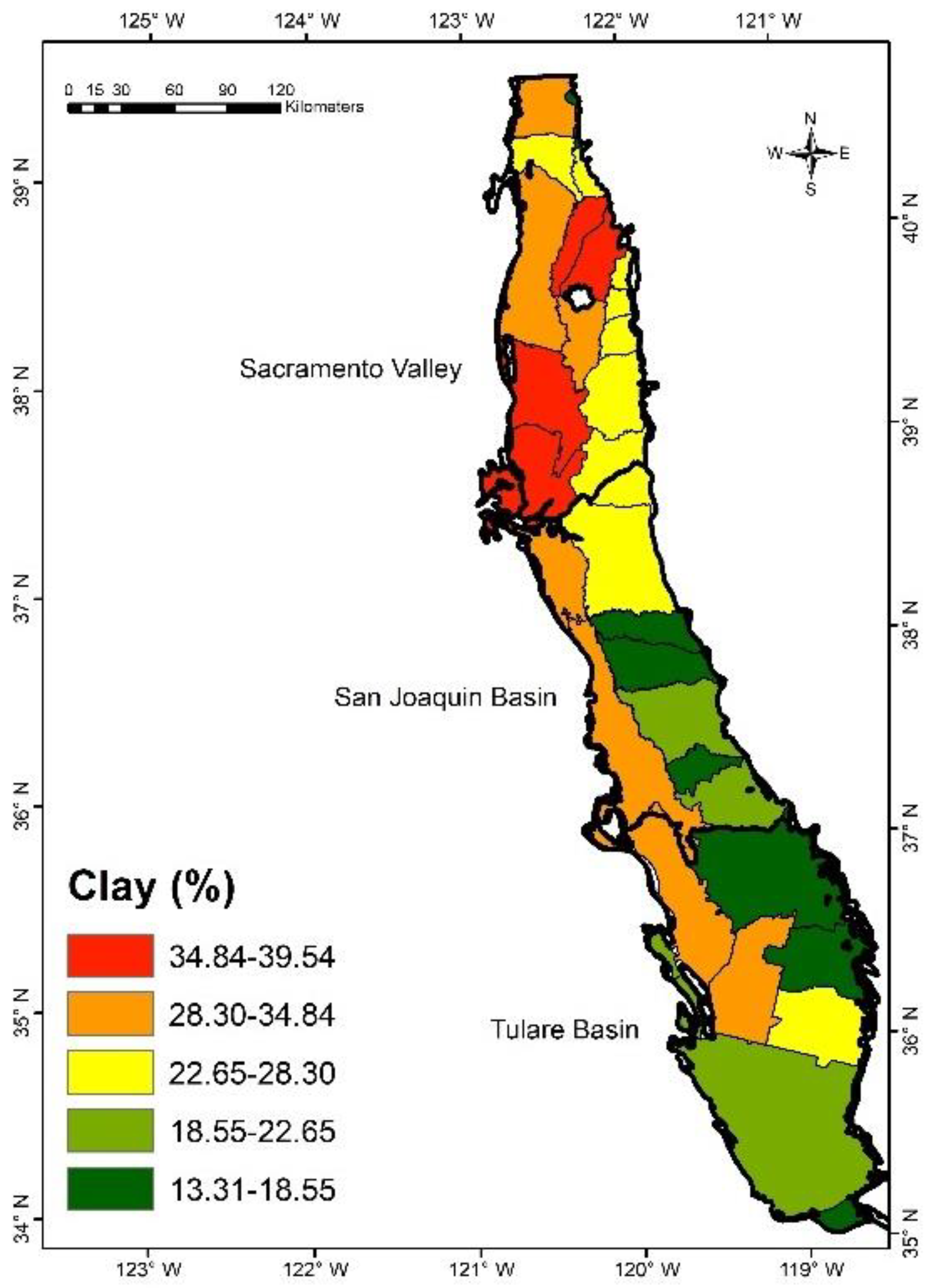
We borrowed the Frequency- Ratio method from the landslide susceptibility method, which has been successfully applied in many landslides susceptibility studies. In the GFR method, Geodetector identifies precipitation, fertilizer, manure, elevation, and clay as the significant variables among twelve different variables and have direct spatial association with the distribution of the contaminated wells in the CV [26]. Although, in this study, Geodetector utilized only 12 different explanatory variables to compute the PD values, the method can process any number of potential explanatory variables to determine their relevance based on the computed PD values and significance tests. In addition, this method can process both categorical and continuous variables, which makes it possible to include wider variety of potential explanatory variables. Furthermore, this method makes no assumptions about the data making it suitable to process nitrate data which are mostly skewed data as they are found in low concentration in normal condition. The GFR method offers a general framework for objectively selecting contributing factors (based on the significance test of PD values) and assigning their weights (based on normalized PD values), which can potentially be applied to any other study areas. Thus, GFR method is more effective than optimized- DRASTIC method for accurately capturing the vulnerability of groundwater contamination, as illustrated in this study in the CV aquifer.

The results of this study are comparable to the findings of previous studies performed in the CV. Ransom et al. [69] also found higher nitrate concentration in wells of San Joaquin and Tulare Basin than Sacramento valley. The Sacramento Valley is composed of fine grained sediments compared to southern part of the CV, which could reduce the susceptibility of Sacramento Valley. There are several studies which modify DRASTIC method by adding the variables or changing the intervals to assign rating values matching the site-specific condition. However, they are mostly site specific, whereas the GFR method offers a general framework that can be applied anywhere.

In this study, a total of 31 groundwater basins were observed with contaminated wells (>5 mg/L) out of 41 basins in the CV. The advantage of the groundwater susceptibility mapping using overlay–index approach is that a vulnerability index value can be calculated for all the basins using the rating and weight values [70]. The visual comparison of two vulnerability index maps showed that optimized-DRASTIC method produced generally a higher index value in the eastern flank of the valley, while the GFR index was higher in San Joaquin and Tulare Basins. However, the GFR method was found to be more consistent with observed contamination data than the optimized-DRASTIC method, as measured by the Pearson’s correlation coefficient and the PD value between the vulnerability index and percent of contaminated wells in the groundwater basins, which confirmed the validity of the newly developed GFR method. The GFR index values were negatively skewed, showing relatively higher numbers of groundwater basins in the upper range. The spatial variance analysis based Geodetector method was effective and can be used in different areas to measure the spatial association. However, high PD values obtained from the Geodetector method is a statistical output and does not necessarily mean causality. Therefore, we should still be careful in selecting the relevant variables.

5. Conclusions

The Central Valley aquifer of California is a highly productive land, where 75% of the land is used for agriculture. The heavy application of fertilizer and changing hydrogeological condition caused by irrigation has exacerbated the groundwater nitrate contamination over last several decades in the CV. Groundwater nitrate contamination above the EPA MCL in drinking water is a health hazard that could induce several health problems. The optimized-DRASTIC method and GFR method were applied to perform a comparative study on the vulnerability of groundwater nitrate contamination in the valley. The subjectively preassigned hydrogeologic variables and weights in the optimized-DRASTIC method may not accurately reflect the changed hydrogeologic conditions in San Joaquin and Tulare Basins region due to heavy pumping, which could have promoted downward percolation of nitrate in this part of the valley, and thus limited the accuracy of its output map. On the other hand, the GFR method integrated the frequency ratio method, which was proven to be effective in landslide susceptibility studies, and the Geodetector method, which has the ability to objectively select contributing factors (based on the significance test of PD values) and assign their weights (based on normalized PD values), and thus produced a more accurate groundwater contamination vulnerability index map as shown by the Pearson correlation coefficient and Geodetector PD values between the index value and percent of contaminated wells in the groundwater basins. In addition, the Geodetector method in GFR method makes no assumption about the data and works for both categorial and continuous data. These unique properties of GFR method render it an accurate and effective method for the groundwater vulnerability assessment. The GFR method offers water resources managers and policy makers a general framework to assess groundwater contamination vulnerability in any other study areas.

References

1. Faunt, C.C. Groundwater Availability of the Central Valley Aquifer, California; U.S. Geological Survey: Reston, VA, USA, 2009.
2. Rosentock, T.S.; Liptzin, D. Nitrogen fertilizer use in California: Assessing the data, trends and a way forward. Calif. Agric. 2013, 67, 68–79. [Google Scholar] [CrossRef] [Green Version]
3. Harter, T.; Zhang, M.; Tomich, T.P.; Pettygrove, G.S. Nitrogen Fertilizer Loading to Groundwater in the Central Valley; University of California: Berkeley, CA, USA, 2012. [Google Scholar]
4. Harter, T. Nitrates in Groundwater. Southwest Hydrol. 2009, 8. [Google Scholar]
5. Belitz, K.; Fram, M.S.; Johnson, T. Metrics for Assessing the Quality of Groundwater Used for Public Supply, CA, USA: Equivalent-Population and Area. Environ. Sci. Technol. 2015, 49, 8330–8338. [Google Scholar] [CrossRef] [PubMed]
6. California State Water Resources Control Board (CSWRCB). Groundwater Ambient Monitoring and Assessment (GAMA) Domestic Well Project Groundwater Quality Report, Tulare County Focus Area; California State Water Resources Control Board, Groundwater Protection: Sacramento, CA, USA, 2016. [Google Scholar]
7. Lockhart, K.; King, A.M.; Harter, T. Identifying sources of groundwater nitrate contamination in a large alluvial groundwater basin with highly diversified intensive agricultural production. J. Contam. Hydrol. 2013, 151, 140–154. [Google Scholar] [CrossRef] [PubMed]
8. Burrow, K.R.; Shelton, J.L.; Dubrovsky, N.M. Occurrence of Nitrate and Pesticide in Ground Water Beneath Three Agricultureal Land-Use Settings in the Eastern San Joaquin Valley, California, 1993–1995; U.S. Geological Survey: Sacramento, CA, USA, 1998.
9. Belitz, K.; Dubrovsky, N.M.; Burrow, K.R.; Jurgens, B.C.; Johnson, T. Framework for a Ground-Water Quality Monitoring and Assessment Program for California; U.S. Geological Survey: Reston, VA, USA, 2003; p. 78.
10. Anning, D.W.; Paul, A.P.; McKinney, T.S.; Huntington, J.M. Predicted Nitrate and Arsenic Concentrations in Basin-Fill Aquifers of the Southwestern United States; National Water-Quality Assessment Program: Reston, VA, USA, 2012. [Google Scholar]
11. Rosecrans, C.Z.; Nolan, B.T.; Gronberg, J.M. Prediction and visualization of redox conditions in the groundwater of Central Valley, California. J. Hydrol. 2017, 546, 341–356. [Google Scholar] [CrossRef]
12. Neukum, C.; Azzam, R. Quantitative assessment of intrinsic groundwater vulnerability to contamination using numerical simulations. Sci. Total Environ. 2009, 408, 245–254. [Google Scholar] [CrossRef] [PubMed]
13. Javadi, S.; Kavehkar, N.; Mousavizadeh, M.H.; Mohammadi, K. Modification of DRASTIC Model to Map Groundwater Vulnerability to Pollution Using Nitrate Measurements in Agricultural Areas. J. Agric. Sci. Technol. 2011, 13, 239–249. [Google Scholar]
14. Li, R.; Merchant, J.W.; Chen, X.-H. A Geospatial Approach for Assessing Groundwater Vulnerability to Nitrate Contamination in Agricultural Settings. Water Air Soil Pollut. 2014, 225, 2214. [Google Scholar] [CrossRef]
15. Baker, R.J.; Chepiga, M.M.; Cauller, S.J. Median Nitrate Concentrations in Groundwater in the New Jersey Highlands Region Estimated Using Regression Models and Land-Surface Characteristics; U.S. Geological Survey: Reston, VA, USA, 2015; p. 27.
16. Gardner, K.; Vogel, R.M. Predicting ground water nitrate concentration from land use. Groundwater 2005, 43, 343–352. [Google Scholar] [CrossRef] [PubMed] [Green Version]
17. Nolan, B.T.; Gronberg, J.M.; Faunt, C.C.; Eberts, S.M.; Belitz, K. Modeling Nitrate at Domestic and Public-Supply Well Depths in the Central Valley, California. Environ. Sci. Technol. 2014, 48, 5643–5651. [Google Scholar] [CrossRef] [PubMed]
18. Nolan, B.T.; Hitt, K.J.; Ruddy, B.C. Probability of Nitrate Contamination of Recently Recharged Groundwaters in the Conterminous United States. Environ. Sci. Technol. 2002, 36, 2138–2145. [Google Scholar] [CrossRef] [PubMed] [Green Version]
19. Burrow, K.R.; Nolan, B.T.; Rupert, M.G.; Dubrovsky, N.M. Assessment of regional change in nitrate concentrations in groundwater in the Central Valley, California, USA, 1950s–2000s. Environ. Earth Sci. 2012, 69, 2609–2621. [Google Scholar] [CrossRef]
20. Lindsey, B.D.; Rupert, M.G. Methods for Evaluating Temporal Groundwater Quality Data and Results of Decadal-Scale Changes in Chloride, Dissolved Solids, and Nitrate Concentrations in Groundwater in the United States 1988–2010; U.S. Geological Survey: Reston, VA, USA, 2012.
21. Aller, L.; Lehr, J.H.; Petty, R. Drastic A Standardized System for the Evaluating Groundwater Pollution Using Hydrogeologic Settings; US Environmental Protection Agency: Oklahoma City, OK, USA, 1987.
22. Ghazavi, R.; Ebrahimi, Z. Assessing groundwater vulnerability to contamination in an arid environment using DRASTIC and GOD models. Int. J. Environ. Sci. Technol. 2015, 12, 2909–2918. [Google Scholar] [CrossRef] [Green Version]
23. Maria, R. Comparative studies of groundwater vulnerability assessment. In IOP Conference Series: Earth and Environmental Science; IOP: London, UK, 2018; Volume 118. [Google Scholar]
24. Al-Rawabdeh, A.M.; Al-Ansari, N.A.; Al-Taani, A.A.; Knutsson, S. A GIS-Based Drastic Model for Assessing Aquifer Vulnerability in Amman-Zerqa Groundwater Basin, Jordan. Engineering 2013, 5, 490–504. [Google Scholar] [CrossRef]
25. Samara, T.; Yoxas, G. Drastic Method to map groundwater vulnerability to poolution using nitrate measurement in agricultural areas. Bull. Geol. Soc. Greece 2013, 47, 981–991. [Google Scholar] [CrossRef]
26. Shrestha, A.; Luo, W. An assessment of groundwater contamination in Central Valley aquifer, California using geodetector method. Ann. GIS 2017, 23, 149–166. [Google Scholar] [CrossRef]
27. Tiwari, A.K.; Singh, P.K.; Maio, M.D. Evaluation of aquifer vulnerability in a coal mining of India by using GIS-based DRASTIC model. Arab. J. Geosci. 2016, 9, 438. [Google Scholar] [CrossRef]
28. Ghosh, A.; Tiwari, A.K.; Das, S. A GIS based DRASTIC model for assessing groundwater vulnerability of Katri Watershed, Dhanbad, India. Model. Earth Syst. Environ. 2015, 1, 11. [Google Scholar] [CrossRef]
29. Antonakos, A.; Lambrakis, N.J. Development and testing of three hybrid methods for the assessment of aquifer vulnerability to nitrates, based on the drastic model, an example from NE Korinthia, Greece. J. Hydrol. 2007, 333, 288–304. [Google Scholar] [CrossRef]
30. Merchant, J.W. GIS-Based Gtoundwater Pollution Hazad Assessment: A Critical Review of the DRASTIC Mode. Photogramm. Eng. Remote Sens. 1994, 60, 1117–1127. [Google Scholar]
31. Kazakis, N.; Voudouris, K.S. Groundwater vulnerability and pollution risk assessment of porous aquifers to nitrate: Modifying the DRASTIC method using quantitative parameters. J. Hydrol. 2015, 525, 13–25. [Google Scholar] [CrossRef]
32. Rupert, M.G. Improvements to the DRASTIC Ground-Water Vulnerability Mapping Method; U.S. Geological Survey: Reston, VA, USA, 1999.
33. Luo, W.; Jasiewicz, J.; Stepinski, T.; Wang, J.-F.; Cang, X. Spatial association between dissection density and environmental factors over the entire conterminous United States. Geophys. Res. Lett. 2016, 43, 692–700. [Google Scholar] [CrossRef] [Green Version]
34. Rasyid, A.R.; Bhandary, N.P.; Yatabe, R. Performance of frequency ratio and logistic regression model in creating GIS based landslides susceptibility map at Lompobattang Mountain, Indonesia. Geoenviron. Diasters 2016, 3, 19. [Google Scholar] [CrossRef]
35. Teimouri, M.; Graee, P. Evaluation of AHP and Frequency Ratio Methods in Landslide Hazard Zoning (Case Study: Bojnord Urban Watershed, Iran). Int. Res. J. Appl. Basic Sci. 2012, 3, 1978–1984. [Google Scholar]
36. Neshat, A.; Pradhan, B. An integrated DRASTIC model using frequency ratio and two new hybrid methods for groundwater vulnerability assessment. Nat. Hazards 2015, 76, 543–563. [Google Scholar] [CrossRef]
37. Luo, W.; Liu, C.-C. Innovative landslide susceptibility mapping supported by geomorphon and geographical detector methods. Landslides 2018, 15, 465–474. [Google Scholar] [CrossRef]
38. Williamson, A.; Prudic, D.; Swain, L.A. Ground-Water Flow in the Central Valley, California; US Government Printing Office: Washington, DC, USA, 1989.
39. Planert, M.; Williams, J.S. Ground Water Atlas of the United States: Segment 1, California, Nevada; U.S. Geological Survey: Reston, VA, USA, 1995.
40. Galloway, D.; Riley, F.S. San Joaquin Valley, California: Largest human alteration of the Earth’s surface. In Land Subsidence in the United States; US Geological Survey: Reston, VA, USA, 1999; Volume 1182, pp. 23–34. [Google Scholar]
41. California Department of Water Resources. Available online: https://gis.water.ca.gov/app/gicima/ (accessed on 8 August 2017).
42. California Department of Water Resources, Groundwater Bain Boundary Assessment Tool. Available online: https://www.mojavewater.org/geospatial-library.html (accessed on 10 April 2018).
43. Mueller, D.K.; Helsel, D.R. Nutrients in the Nation’s Water—Too Much of a Good Thing; USGS Circular 1136; U.S. Geological Survey: Reston, VA, USA, 1996; 24p.
44. Ward, M.H.; DeKok, T.M.; Levallois, P.; Brender, J.; Gullis, G.; Nolan, B.T.; VanDerslice, J. Workgroup report: Drinking-Water Nitrate and Health—Recent Findings and Research Needs. Environ. Health Perspect. 2005, 113, 1607–1614. [Google Scholar] [CrossRef] [Green Version]
45. Klug, J. Modeling the Risk of Groundwater Contamination Using DRASTIC and Geographic Information Systems in Houston County, Minnesota. In Papers in Resource Analysis; Saint Mary’s University of Minnesota: Winona, MN, USA, 2009; Volume 11, p. 12. [Google Scholar]
46. Wolock, D.M. Estimated Mean Annual Natural Ground-Water Recharge in the Conterminous United States; U.S. Geological Survey Open-File Report; U.S. Geological Survey: Reston, VA, USA, 2003.
47. McKinney, T.S. Surficial Geology of the Southwest Principal Aquifers (SWPA) Study; Scientific Investigation Report; U.S. Geological Survey: Reston, VA, USA, 2008. [Google Scholar]
48. Schwarz, G.E.; Alexander, R.B. Soils Data for the Conterminous United States Derived from the NRCS State Soil Geographic (STATSGO) Data Base; Series Name Open-File Report Issue Identification 95-449; U.S. Geological Survey: Reston, VA, USA, 1995.
49. Elevation Derivatives for National Applications (EDNA). Available online: https://edna.usgs.gov/ (accessed on 5 March 2017).
50. Wieczorek, M.E. Area- and Depth-Weighted Averages of Selected SSURGO Variables for the Conterminous United States and District of Columbia; U.S. Geological Survey Data Series; U.S. Geological Survey: Reston, VA, USA, 2014.
51. Piscopo, G. Groundwater Vulnerability Map Explanatory Map-Castelreagh Catchment; NSW Department of Land and Water Conservation: Kingswood, Australia, 2001. [Google Scholar]
52. Kumar, V. Remadevi Kriging of groundwater levels—A case study. J. Spat. Hydrol. 2006, 6, 81–92. [Google Scholar]
53. Sun, Y.; Kang, S.; Fusheng, L.; Zhang, L. Comparison of interpolation methods for depth to groundwater and its temporal and spatial variations in the Minqin oasis of northwest China. J. Environ. Model. Softw. 2009, 24, 1163–1170. [Google Scholar] [CrossRef]
54. Geologic Map of California. Available online: http://maps.conservation.ca.gov/cgs/gmc/ (accessed on 15 April 2018).
55. Wang, J.-F.; Li, X.-H.; Christakos, G.; Liao, Y.-L.; Zhang, T.; Zheng, X.-Y. Geographical Detectors-Based Health Risk Assessment and its Application in the Neural Tube Defects Study of the Heshun Region, China. Int. J. Geogr. Inf. Sci. 2010, 24, 107–127. [Google Scholar] [CrossRef]
56. Shrestha, A.; Luo, W. Analysis of Groundwater Nitrate Contamination in the Central Valley: Comparison of the Geodetector Method, Principal Component Analysis and Geographically Weighted Regression. Int. J. Geo-Information 2017, 6, 297. [Google Scholar] [CrossRef]
57. Gronberg, J.A.M.; Saphr, N.E. County-Level Estimate of Nitrogen and Phosphorus from Commercial Fertilizer for the Conterminous United States, 1987–2006; U.S. Geological Survey: Reston, VA, USA, 2012.
58. Mueller, D.K. County-Level Estimates of Nitrogen and Phosphorus from Animal Manure for the Conterminous United States, 2002; U.S. Geological Survey: Reston, VA, USA, 2013.
59. Homer, C.G.; Dewitz, J.A.; Yang, L.; Jin, S.; Danielson, P.; Xian, G.; Coulston, J.; Herold, N.D.; Wickham, J.D.; Megown, K. Completion of the 2011 National Land Cover Database for the conterminous United States-Representing a decade of land cover change information. Photogramm. Eng. Remote Sens. 2015, 81, 346–354. [Google Scholar]
60. Wolock, D.M. STATSGO Soil Characteristics for the Conterminous United States; U.S. Geological Survey: Reston, VA, USA, 1997.
61. PRISM Climate Data. Available online: http://www.prism.oregonstate.edu/ (accessed on 10 May 2016).
62. National Elevation Dataset (NED). Available online: http://edna.usgs.gov/Edna/edna.asp (accessed on 16 March 2013).
63. Nolan, B.T.; Hitt, K.J. Vulnerability of shallow ground water and drinking-water wells to nitrate in the United States: Model of predicted nitrate concentration in shallow, recently recharged ground water—Input data set for clay sediment (gwava-s_clay). Environ. Sci. Technol. 2006, 40, 7834–7840. [Google Scholar] [CrossRef] [PubMed]
64. National Water-Quality Assessment (NAWQA). Available online: https://water.usgs.gov/nawqa/ (accessed on 25 August 2013).
65. National Water Information System (NWIS). Available online: https://waterdata.usgs.gov/nwis (accessed on 25 August 2013).
66. Lee, S.; Pradhan, B. Probabilistic landslide hazards and risk mapping on Penang Island, Malaysia. J. Earth Syst. Sci. 2006, 115, 661–672. [Google Scholar] [CrossRef]
67. Bertoldi, G.L.; Johnston, R.H.; Evenson, K.D. Ground Water in the Central Valley, California a Summary Report; U.S. Geological Survey: Reston, VA, USA, 1991.
68. Cao, F.; Ge, Y.; Wang, J.-F. Optimal discretization of geographical detector-based risk assessment. GISci. Remote Sens. 2013, 50, 78–92. [Google Scholar]
69. Ransom, K.M.; Nolan, B.T.; Traum, J.A.; Harter, T. A hybrid machine learning model to predict and visualize nitrate concentration throughout the Central Valley aquifer, California, USA. Sci. Total Environ. 2017, 601–602, 1160–1172. [Google Scholar] [CrossRef] [PubMed]
70. Osborn, N.I.; Hardy, R.H. Statewide Groundwater Vulnerability Map of Oklahoma; Oklahoma Water Resources Board: Oklahoma City, OL, USA, 1999. [Google Scholar]
Figure 1. Central Valley Aquifer System.
Ijgi 07 00211 g001
Figure 2. Cross-section of San Joaquin Valley during predevelopment (top) and post-development (bottom) period. Figure from reference [40].
Ijgi 07 00211 g002
Figure 3. Groundwater basins and well samples in Central Valley.
Ijgi 07 00211 g003
Figure 4. Distribution of depth to water in Central Valley.
Ijgi 07 00211 g004
Figure 5. Recharge rate in Central Valley.
Ijgi 07 00211 g005
Figure 6. Aquifer media in Central Valley (see Table 3 for details on Geocodes).
Ijgi 07 00211 g006
Figure 7. Soil Media in Central Valley.
Ijgi 07 00211 g007
Figure 8. Percent slope in Central Valley.
Ijgi 07 00211 g008
Figure 9. Impact of Vadose Zone in Central Valley.
Ijgi 07 00211 g009
Figure 10. Hydraulic Conductivity in Central Valley.
Ijgi 07 00211 g010
Figure 11. DRASTIC Susceptibility Index in Central Valley.
Ijgi 07 00211 g011
Figure 12. Precipitation distribution in Central Valley. (Data: 1981–2010).
Ijgi 07 00211 g012
Figure 13. Fertilizer loading in Central Valley.
Ijgi 07 00211 g013
Figure 14. Manure Loading in Central Valley.
Ijgi 07 00211 g014
Figure 15. Elevation in Central Valley.
Ijgi 07 00211 g015
Figure 16. Percent clay in Central Valley.
Ijgi 07 00211 g016
Figure 17. GFR Susceptibility Index.
Ijgi 07 00211 g017
Figure 18. Histogram of DRASTIC Index values.
Ijgi 07 00211 g018
Figure 19. Histogram of GFR Index Values.
Ijgi 07 00211 g019