Semi-Supervised Ground-to-Aerial Adaptation with Heterogeneous Features Learning for Scene Classification

Abstract

Currently, huge quantities of remote sensing images (RSIs) are becoming available. Nevertheless, the scarcity of labeled samples hinders the semantic understanding of RSIs. Fortunately, many ground-level image datasets with detailed semantic annotations have been collected in the vision community. In this paper, we attempt to exploit the abundant labeled ground-level images to build discriminative models for overhead-view RSI classification. However, images from the ground-level and overhead view are represented by heterogeneous features with different distributions; how to effectively combine multiple features and reduce the mismatch of distributions are two key problems in this scene-model transfer task. Specifically, a semi-supervised manifold-regularized multiple-kernel-learning (SMRMKL) algorithm is proposed for solving these problems. We employ multiple kernels over several features to learn an optimal combined model automatically. Multi-kernel Maximum Mean Discrepancy (MK-MMD) is utilized to measure the data mismatch. To make use of unlabeled target samples, a manifold regularized semi-supervised learning process is incorporated into our framework. Extensive experimental results on both cross-view and aerial-to-satellite scene datasets demonstrate that: (1) SMRMKL has an appealing extension ability to effectively fuse different types of visual features; and (2) manifold regularization can improve the adaptation performance by utilizing unlabeled target samples.

1. Introduction

With the rapid increase in remote sensing imaging techniques over the past decade, a large amount of very high-resolution (VHR) remote sensing images are now accessible, thereby enabling us to study ground surfaces in greater detail [1,2,3,4,5]. Recent studies often adopt the bag-of-visual-words (BOVW) [6,7,8] or deep convolutional neural networks (DCNN) representation [9,10,11,12,13,14,15,16,17,18] associated with AdaBoost classifiers or support vector machine (SVM) classifiers to learn scene class models. The collection of reference samples is a key component for a successful classification of the land-cover classes. However, in real-world earth observation (EO) applications, the available labeled samples are not sufficient in number, which hinders the semantic understanding of remote sensing images. Directly addressing this problem is challenging because the collection of labeled samples for newly acquired scenes is expensive and the labeling process involves time-consuming human photo interpretation that cannot follow the pace of image acquisition. Instead of collecting semantic annotations for remote sensing images, some research has considered strategies of adaptation, which is a rising field of investigation in the EO community since it meets the need for reusing available samples to classify new images. Tuia et al. [19] provided a critical review of recent domain adaptation methodologies for remote sensing and divided them into four categories: (1) invariant feature selection; (2) representation matching; (3) adaptation of classifiers; and (4) selective sampling. Nevertheless, all these methods [20,21,22,23,24] are designed for annotation transfer between remote sensing images. With an increasing amount of freely available ground level images with detailed tags, one interesting and possible intuition is that we can train semantic scene models using ground view images, as they have already been collected and annotated, and hope that the models still work well on overhead-view aerial or satellite scene images. In detail, ground view represents the natural scene images taken from the ground view. Overhead view represents the remote sensing images taken from the overhead view, which contains overhead aerial scene images and overhead satellite scene images.

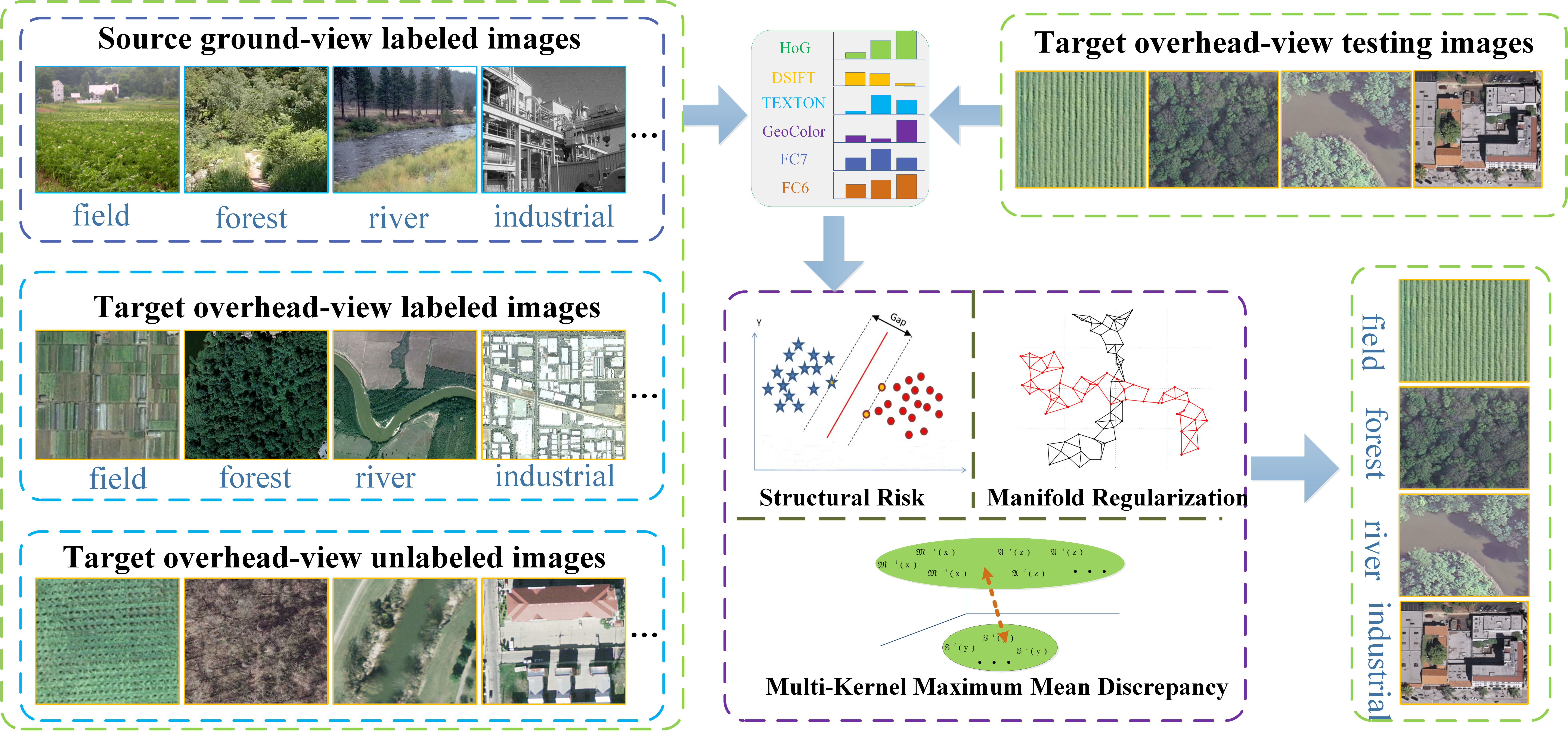
Transferring semantic category models from the ground view to the overhead view has two advantages: First, ground-view and overhead-view images are classified under the same scene class despite being captured from two different views, leading to consistency in the underlying intrinsic semantic features. Second, large-scale ground-view image datasets such as ImageNet [25] and SUN [26] have been built with detailed annotations that have fostered many efficient ways to describe the image semantically. However, the generalization of the classifiers pre-trained from ground level annotations is not guaranteed, as training and testing samples are drawn from different probability distributions. To solve this problem, on the one hand, several works have addressed the cross-view (ground-to-aerial) domain adaption problem in the context of image geolocalization [27]. On the other hand, the work of [28,29,30,31,32] must be mentioned, as the authors aim to transfer scene models from ground to aerial based on the assumption that scene transfer is a special case of cross-domain adaptation, where the divergences across domains are caused by viewpoint changes, somewhat similar in spirit to our work. However, all these methods are feature learning-based adaptation approaches, where ground view and overhead view data are represented by one kind of feature, such as the histogram of oriented edges (HOG) feature. Nevertheless, multiple features should be considered because the elements in the same scene captured from two different views may appear at different scales and orientations. Because different types of features describe different visual aspects, it is difficult to determine which feature is better for adaptation. When considering heterogeneous types of features with different dimensions, scene model transfer deals with an even more challenging task. Figure 1 illustrates the appearance of considerable discrepancy in the same residential class captured from four views. Six types of features of each image are projected onto two dimensions using t-Distributed Stochastic Neighbor Embedding (t-SNE) [33] with different colors. The solid points, hexagram points, represent the residential class images captured from different views. The complexity of different features and the distinct distributions between different views pose great challenges to adaptive learning schemes.

Techniques for addressing the mismatched distributions of multiple types of features with different dimensions have been investigated under the names of heterogeneous domain adaptation (HDA). Most existing HDA approaches were feature representation-based methods whose aim is to make the data distributions more similar across the domains [21,34,35]. However, these methods are suitable for transfer tasks with limited deformations, whereas the difference between cross-view images are huge. With the rapid development of deep neural networks, more recent works use deep adaptation methods [36,37] to reduce the domain shift, which brings new insights into our cross view scene model transfer task. However, deep adaptation-based approaches involve a large number of labeled samples to train the network in a reasonable time [38]. Generally, the ground-view domain contains a large amount of labeled data such that a classifier can be reliably built, while the labeled overhead view data are often very few and they alone are not sufficient to construct a good classifier. Thus, based on the guidelines for choosing the adaptation strategy in [19], we focus on the classifier adaptation methods that can utilize the source domain models as prior knowledge to learn the target model. However, due to the huge domain mismatch between ground view images and overhead view images, three problems need to be solved for better adaptation: (1) how to fuse multiple features for cross-view adaptation; (2) how to reduce the mismatch of multiple feature distribution between cross-view domains; and (3) how to effectively leverage unlabeled target data to improve the adaptation performance.

To address these issues, in this paper, we propose a semi-supervised manifold-regularized multiple-kernel-learning (SMRMKL) algorithm to transfer scene models from ground-to-aerial. To fuse heterogeneous types of image features, we employ multiple kernels to map samples to the corresponding Reproducing Kernel Hilbert Space (RKHS), where multi-kernel maximum mean discrepancy (MK-MMD) is utilized to reduce the mismatch of data distributions between cross-view domains. To make use of available unlabeled target samples, we incorporate a manifold-regularized local regression on target domains to capture the local structure for scene model transfer. After iterative optimization of the unified components by the reduced gradient descent procedure, we obtain an adapted classifier for each scene class; then, a new coming target sample’s label can be determined accordingly. Extensive experimental results on both aerial-to-satellite, and ground-to-aerial or -satellite scene image datasets demonstrate that our proposed framework improves the adaptation performance by fusing different types of visual features and utilizing unlabeled target samples.

The rest of this paper is organized as follows. Section 2 presents our manifold-regularized multiple kernel learning framework. Section 3 reports the experimental results. Finally, Section 4 concludes the paper.

2. Semi-Supervised Manifold-Regularized Multiple Kernel Learning

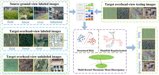
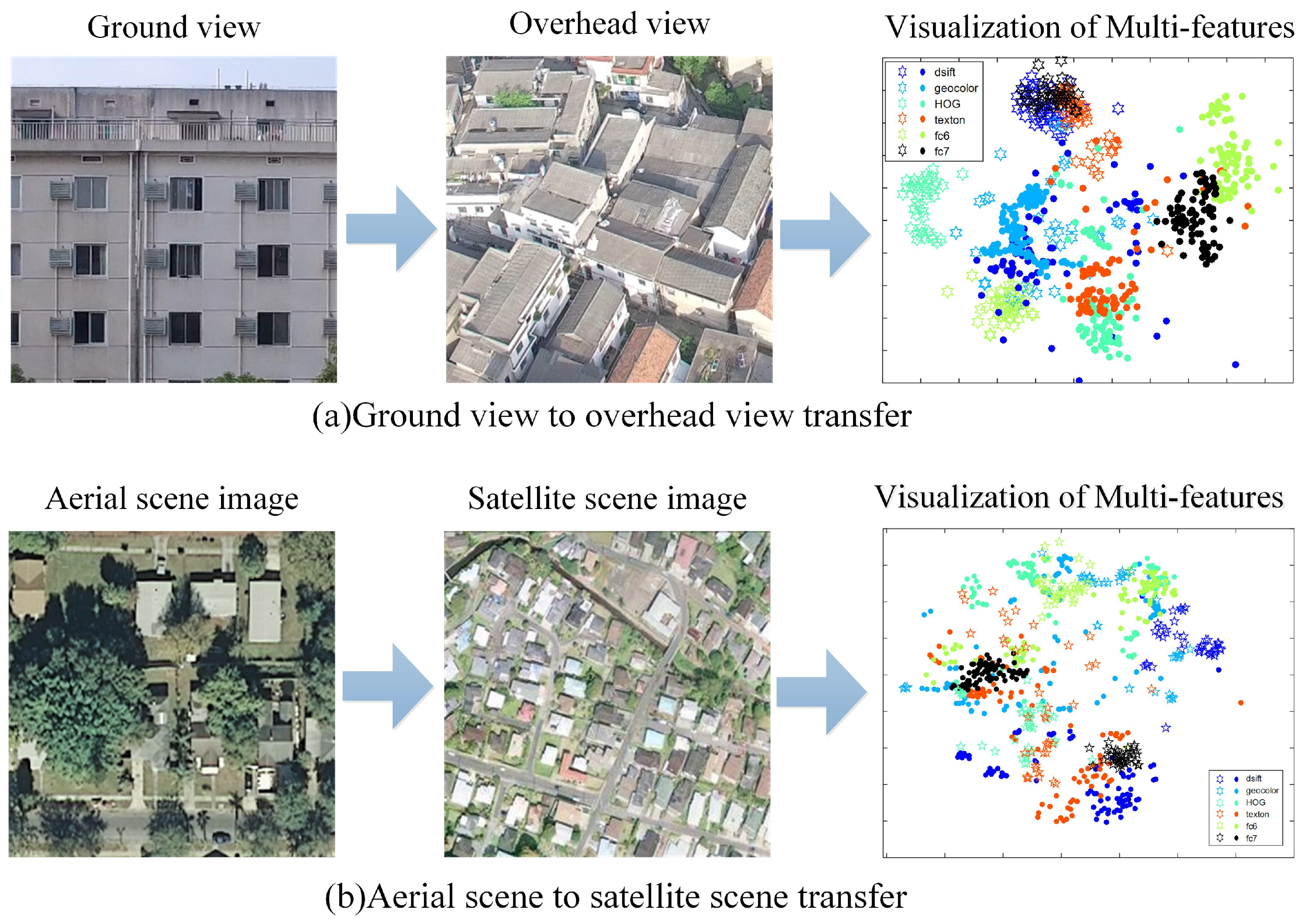
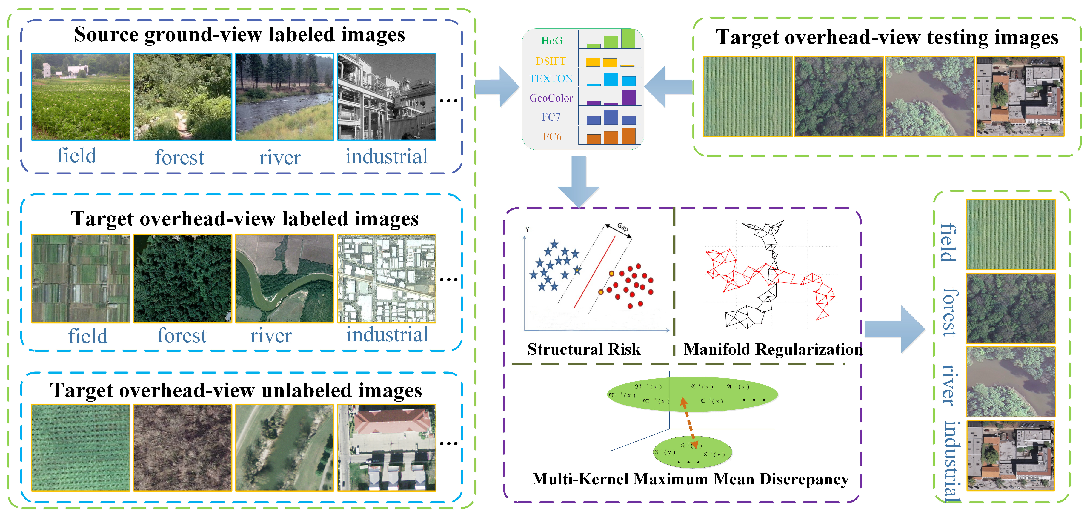
We construct the cross-view scene model transfer task as a classifier adaptation-based HDA problem. To be more precise, many labels are available for the source domain, and only a few labels are provided for the target domain. Taking the ground view image set as the source domain and the overhead view image set to be learned as the target domain, we want to adapt the scene model categories in the label-rich source domain to the label-scarce target domain. The main goal of SMRMKL is to bridge the cross-view domain gap by jointly learning adaptive classifiers and transferable features to minimize domain divergence. As shown in Figure 2, three regularizers are jointly employed in our framework, including the MK-MMD to match feature distributions for feature adaptation; the structural risk regularizer, which corresponds to an empirical risk minimization that makes SVM exhibit good generalization; and the manifold regularizer based on the basic intuition that the closer target unlabeled samples in the feature space may contain similar decision values. In the following, we will first introduce the notations used in this paper, followed by constructing the three regularizers of SMRMKL. Then, the optimization strategy of the overall objective is provided.

2.1. Notations

For simplicity, we focus on the scenario where there is one source domain $D^S$ and one target domain $D^T$. Taking the ground-view scene image set with plenty of labels as the source domain $D^S=({x_i}^S,{y_i}^S){|}_{i=1}^{n_S}$ , where ${y_i}^S$ indicates the corresponding label of image ${x_i}^S$ and $n_S$ is the size of $D^S$. Similarly, let $D^T={D_l}^T\cup {D_u}^T$ denote the overhead-view remote sensing image set of the target domain with a limited number of labeled data and a large number of un-labeled data, where ${D_l}^T=({x_i}^T,{y_i}^T){|}_{i=1}^{n_l}$ and ${D_u}^T={x_i}^T{|}_{i=n_l+1}^{n_l+n_u}$ represent the labeled and unlabeled training images, respectively. The size of $D^T$ is $n_T=n_l+n_u(n_l\ll n_u)$. We define $N=n_S+n_T$ and $n=n_S+n_l$ as denoting the size of all training data and labeled training data from both domains, respectively. It is assumed that both the ground level images and remote sensing images pertain to J categories, i.e., they share the same label space. Our goal is to learn from $\left\{D^S\right.,\left.D^T\right\}$ a scene model decision function $f^T(x)$ that predicts the label of a novel test sample from the remote sensing domain.

2.2. Multi-Kernel Maximum Mean Discrepancy

In this section, we investigate how to bridge the source-target discrepancy in the feature space. The broad variety of cross-view images requires different types of features to describe different visual aspects, such as the color, texture and shape. Furthermore, with the development of deep neural networks, the output feature (i.e., deep feature) of convolutional layer or fully collected layer can represent image in a hierarchical way. As shown in Figure 3, each image is represented by different features with different dimensions. To overcome the problem of diversity, kernel methods have been extensively studied to minimize the mismatch of different distributions and combine different data modalities. In this paper, we use the nonparametric criterion called MMD to compare data distributions based on the distance between means of samples from two domains in a Reproducing Kernel Hilbert Space (RKHS), which has been shown to be effective in domain adaptation. The criterion of MMD is:

$$DIST({D_i}^S,{D_i}^T)=∥\frac{1}{n_S}\sum _{i=1}^{n_S}\phi ({x_i}^S)-\frac{1}{n_T}\sum _{i=1}^{n_T}\phi ({x_i}^T)∥$$

(1)

where ${x_i}^S$ and ${x_i}^T$ are images from the source and target domains, respectively, and $∥•∥$ denotes the $l_2$ norm. A kernel function K is induced from the nonlinear feature mapping function $\phi (•)$, i.e., $K(x_i,x_j)=\phi {(x_i)}^{\prime }\phi (x_j)$. To simplify the MMD criterion, we defined a column vector

$$q={[\underset{n_S}{\underbrace{1/n_S,\dots ,1/n_S}},\underset{{\mathrm{n}}_T}{\underbrace{-1/{\mathrm{n}}_T,\dots -1/{\mathrm{n}}_T}}]}^{\prime }$$

to transform Equation (1) to:

$$DIST({D_i}^S,{D_i}^T)=tr(KQ)$$

(2)

where $Q=q{q}^{\prime }\in {\Re }^{N\times N}$, $K=[\begin{array}{cc}{K}_{SS}& K_{ST}\\ K_{TS}& K_{TT}\end{array}]\in {\Re }^{N\times N}$, $K_{SS}$, $K_{TT}$ and $K_{ST}$ are the kernel matrices defined for the source domain, target domain, and the cross-domain from the source images to the target images, respectively.

To effectively fuse multiple types of features for cross-view scene model transfer task, we employ multiple kernel learning method to construct the kernel matrices by a linear combination of different feature kernels matrices $K^{(m)}$.

$$K=\sum _{m=1}^M{d}_m{K}^{(m)}$$

(3)

where $d_m$ are the linear combination coefficients and ${\displaystyle {\displaystyle \sum }_{m=1}^M}{d}_m=1$. $K^{(m)}(m=1,2,\dots ,M)$ is a base kernel matrix that combines both source and target images derived from different feature mapping functions $\phi (•)$. Thus, the MK-MMD criterion is simplified:

$$DIS{T}_K(D^S,D^T)=tr(\sum _{m=1}^M{d}_m{K}^{(m)}Q)=p^{\prime }d$$

(4)

where $p={[tr(K^{(1)}Q),\dots ,tr(K^{(m)}Q)]}^{\prime }$ and $d={[d_1,\dots ,d_M]}^{\prime }$ is the vector of kernel combination coefficients. When we minimize $DIS{T}_K(D^S,D^T)$ to be close to zero, the data distributions of the two domains are close to each other.

2.3. Structural Risk

In this section, we investigate how to bridge the discrepancy of source classifier $f^S(x)$ and target classifier $f^T(x)$. Previous works [39] assume that $f^T(x)=f^S(x)+\Delta f(x)$, where $\Delta f(x)$ is the perturbation function adapted from the training data. In this paper, we learn a robust target decision function adapted from a combination of pre-learned classifiers and a perturbation function as follows [39]:

$$f^T(x)=f^S(x)+\Delta f(x)={\displaystyle \sum _{p=1}^P}{\beta }_p{f}_p(x)+{\displaystyle \sum _{m=1}^M}{d}_{m}w{}_m^{\prime }{\phi }_m(x)+b$$

(5)

where $f_p(x)$ is the pre-learned classifiers with a linear combination coefficients ${\beta }_p$ trained based on the labeled data from both domains and P is the total number of the pre-learned classifiers. $\Delta f(x)={\displaystyle {\displaystyle \sum }_{m=1}^M}{d}_{m}w{}_m^{\prime }{\phi }_m(x)+b$ is the perturbation function with b as the bias term. $w_m^{\prime }$ and ${\phi }_m(x)$ are the $m_{th}$ kind of normal vector and feature mapping function. Therefore, we form the structural risk functional as follows:

$$\begin{array}{c}\underset{w_m,\beta ,b,{\xi }_i}{min}\frac{1}{2}\left({\displaystyle \sum _{m=1}^M}{d}_m\right.{∥w_m∥}^2+\left.\lambda {∥\beta ∥}^2\right)+C{\displaystyle \sum _{i=1}^n}{\xi }_i\hfill \\ \mathrm{s}.\mathrm{t}.y_i{f}^T(x_i)\ge 1-{\xi }_i,{\xi }_i\ge 0\hfill \end{array}$$

(6)

$\beta ={[{\beta }_1,\dots ,{\beta }_P]}^{\prime }$ is the vector of ${\beta }_p$s, and $\lambda ,C>0$ are the regularization parameters. Denote ${\tilde{v}}_m=d_m{[w_m^{\prime },\sqrt{\lambda }{\beta }^{\prime }]}^{\prime }$, and the optimization problem in Equation (6) can then be computed as follows:

$$\begin{array}{c}\underset{{\tilde{v}}_m,b,{\xi }_i}{min}\frac{1}{2}{\displaystyle \sum _{m=1}^M}\frac{{∥{\tilde{v}}_m∥}^2}{d_m}+C{\displaystyle \sum _{i=1}^n}{\xi }_i\hfill \\ \mathrm{s}.\mathrm{t}.y_i({\displaystyle \sum _{m=1}^M}\tilde{v}{}_m^{\prime }{\tilde{\phi }}_m({\mathrm{x}}_i)+\left.b\right)\ge 1-{\xi }_i,{\xi }_i\ge 0\hfill \end{array}$$

(7)

Denote ${\tilde{\phi }}_m(x_i)={[{\phi }_m{(x_i)}^{\prime },\frac{1}{\sqrt{\lambda }}f{(x_i)}^{\prime }]}^{\prime }$, where $f(x_i)={[f_1(x_i),\dots ,f_P(x_i)]}^{\prime }$, a new kernel matrix $\tilde{K}=[{\tilde{\phi }}_m{(x_i)}^{\prime }{\tilde{\phi }}_m(x_j)]={\displaystyle {\displaystyle \sum }_{m=1}^M}{d}_m{\tilde{K}}^{(m)}=[\begin{array}{cc}{\tilde{K}}_L& {\tilde{K}}_{LU}\\ {\tilde{K}}_{UL}& {\tilde{K}}_U\end{array}]\in {\Re }^{N\times N}$, is defined by the both labeled and un-labeled training data from two domains. ${\tilde{K}}_L=[\begin{array}{cc}{{\tilde{K}}^{SS}}_L& {{\tilde{K}}^{ST}}_L\\ {{\tilde{K}}^{TS}}_L& {{\tilde{K}}^{TT}}_L\end{array}]\in {\Re }^{n\times n}$ is the kernel matrix defined for labeled samples for both two domains. ${\tilde{K}}_U\in {}^{n_u\times n_u}$ and ${\tilde{K}}_{LU}\in {}^{n\times n_u}$ are the kernel matrices defined for the unlabeled samples and cross-domain from the labeled images to the unlabeled images, respectively. Motivated by the optimization problem of SVM, Equation (7) can be solved by its dual problem:

$$\underset{\alpha \in A}{max}{\mathbf{1}}_n^{\prime }\alpha -\frac{1}{2}{(\alpha \circ y)}^{\prime }{\tilde{K}}_L(\alpha \circ y)$$

(8)

where $y={[y_1,\dots ,y_n]}^{\prime }$ is the training samples’ label vector. $A=\left\{\alpha \right|{\alpha }^{\prime }y=0,0_n\le \alpha \le C{\mathbf{1}}_{\mathbf{n}}\}$ is the feasible set of the dual variables $\alpha$.

2.4. Manifold Regularization

In this section, we investigate how to leverage unlabeled target data based on manifold regularization, which has been shown effective for semi-supervised learning [40]. This regularizer’s basic intuition is that the outputs of the predictive function are restricted to assign similar values for similar samples in the feature space. Inspired by Laplacian based semi-supervised learning [41] and Manifold Regularized Least Square Regression (MRLS) [42], the estimation of the manifold regularization can be measured by similarity of the target pairwise samples. Specifically, it can be given by

$$\underset{{\tilde{v}}_m}{min}\sum _{i,j}^{n_T}{S}_{ij}{∥\sum _{m=1}^M{\tilde{v}}_m^{\prime }{\tilde{\phi }}_m({{\mathrm{x}}^T}_i)-\sum _{m=1}^M{\tilde{v}}_m^{\prime }{\tilde{\phi }}_m({{\mathrm{x}}^T}_j)∥}^2$$

(9)

where $S\in n_T\times n_T$ denotes the affinity matrix defined on the target samples, whose element $S_{ij}$ reflects the similarity between ${{\mathrm{x}}^T}_i$ and ${{\mathrm{x}}^T}_j$. By setting the derivative of the Lagrangian obtained from Equation (7) to zero, we can obtain ${\tilde{v}}_m=d_m{\displaystyle {\displaystyle \sum }_{i=1}^n}{\alpha }_i{y}_i{\tilde{\phi }}_m(x_i)$. Thus, Equation (9) can be rewritten as follows:

$$\sum _{i,j}^{n_T}{S}_{ij}{∥\sum _{m=1}^M{d}_m{(\alpha \circ y)}^{\prime }(\tilde{K}(1:n,i+n_S)-\tilde{K}(1:n,j+n_S))∥}^2$$

(10)

One way of computing the elements of affinity matrices S is based on Gaussian functions, i.e.,

$$S_{i,j}=\left\{\begin{array}{c}{e}^{-\frac{{∥{x_i}^T-{x_j}^T∥}^2}{{\sigma }^2}}\\ 0\end{array}\right.\begin{array}{c}\mathrm{if}{x_i}^T\mathrm{and}{x_j}^T\mathrm{are}k\mathrm{nearest}\mathrm{neighbors}\\ else\end{array}$$

(11)

where $\sigma$ is the bandwidth parameter. By defining the graph Laplacian $L=D-S$, where D is a diagonal matrix defined as $D_{ii}={\displaystyle {\displaystyle \sum }_{j=1}^{n_T}}{S}_{ij}$, the manifold regularization can be rewritten as:

$$\begin{array}{c}\hfill ({(\alpha \circ y)}^{\prime }\sum _{m=1}^M{d}_m{\tilde{K}}^{(m)}(1:n,n_S:N))·L({(\alpha \circ y)}^{\prime }\sum _{m=1}^M{d}_m{\tilde{K}}^{(\mathrm{m})}(1:n,n_S:N){)}^T\end{array}$$

(12)

2.5. Overall Objective Function

In this section, we integrate $DIS{T}_K(D^S,D^T)$ in Equation (4) and structural risk functional in Equation (8) into the manifold regularization function in Equation (12) and then arrive at the overall objective function.

$$\begin{array}{c}\hfill G(d)=p^{\prime }d+\theta \left({\mathbf{1}}_n^{\prime }\alpha \right.-\frac{1}{2}{(\alpha \circ y)}^{\prime }{\tilde{K}}_L\left.(\alpha \circ y)\right)+\zeta ({(\alpha \circ y)}^{\prime }\sum _{m=1}^M{d}_m{\tilde{K}}^{(m)}(1:n,n_S:N))L({(\alpha \circ y)}^{\prime }\sum _{m=1}^M{d}_m{\tilde{K}}^{(m)}(1:n,n_S:N){)}^T\end{array}$$

(13)

where $\theta$, $\zeta$ is the trade-off parameter. Thus, we propose an alternating update algorithm to obtain the globally optimal solution. Once we have initialized the linear combination coefficient $d_m$, the optimization problem can be solved by existing SVM solvers such as LIBSVM [43] to obtain the dual variable $\alpha$. Then, the dual variable $\alpha$ is fixed, and the linear combination coefficient $d_m$ is updated by the second-order gradient descent procedure [44] to make the value of the objective function in Equation (13) decrease. Thus, the alternating algorithm of SMRMKL is guaranteed to converge.

3. Experimental Results

We conducted our experiments for both ground-to-aerial scene model adaptation and aerial-to-satellite scene model adaptation.

3.1. Data Set Description and Experimental Configuration

Two couples of source-target image sets were used to evaluate the proposed framework of scene adaptation.

3.1.1. Cross-View Scene Dataset

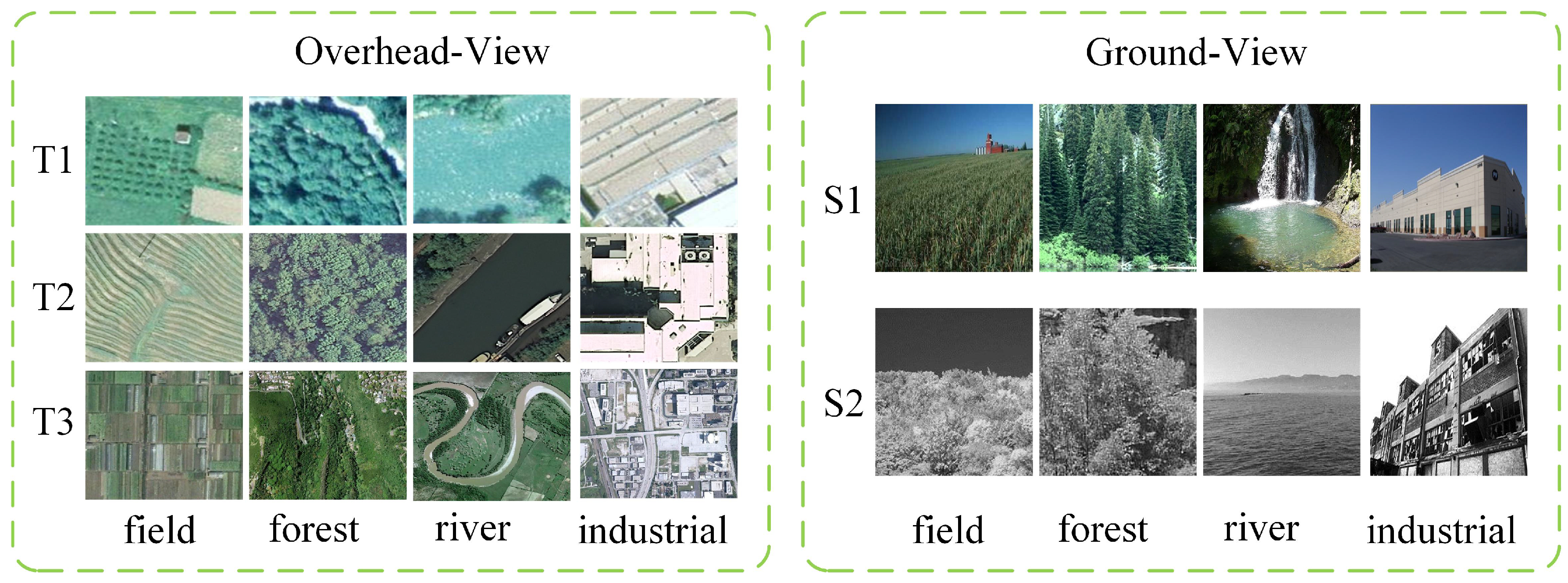
We collected a cross-view scene dataset from two ground-level scene datasets, SUN database (Source domain 1, S1) and Scene-15 [38] (Source domain 2, S2), and three overhead remote sensing scene datasets, Banja Luka dataset [45] (Target domain 1, T1), UC Merced dataset [46] (Target domain 2, T2), and WHU-RS19 dataset [47] (Target domain 3, T3). The Banja Luka dataset consists of 606 RGB aerial images of size $128\times 128$ pixels. The UC Merced dataset is composed of 2100 aerial scene images measuring $256\times 256$ pixels, with a spatial resolution of 0.3 m per pixel in the red green blue color space. The WHU-RS19 dataset was extracted from a set of satellite images exported from Google Earth with spatial resolution up to 0.5 m and spectral bands of red, green, and blue. Our cross-view scene dataset consists of 2768 images of four categories (field/agriculture, forest/trees, river/water and industrial). Figure 4 shows an example of the cross-view scene dataset (one image per class per dataset).

Table 1. Statistical number of images in Cross-view scene dataset. SUN database (S1) and Scene-15 (S2) are the source domains, while Banja Luka (T1), UC Merced (T2), and WHU-RS19 (T3) datasets are the target domains.

	Overhead-View Datasets			Ground-View Datasets
	T1	T2	T3	S1	S2
1 agriculture	178	100	50	84	410
2 forest/trees	105	100	53	62	328
3 river/water	77	100	56	125	360
4 industrial	75	100	53	41	311

gives the statistics of the image numbers in the dataset.

3.1.2. Aerial-to-Satellite Scene Dataset

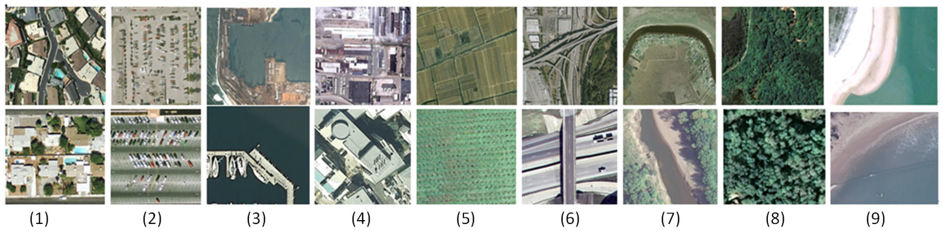
We have collected 1377 images of nine common categories from the UC Merced aerial scene dataset and WHU-RS19 dataset. In this experiment, we use the aerial scene dataset as the source domain, while examples from the satellite scene dataset are used as the target domain training data. In total, there are 900 source training images. Satellite scene dataset has 495 images for all nine categories. Figure 5 shows the images from 9 out of 19 classes.

3.1.3. Base Features and Training/Testing Settings

For images in our two couples of source-target image sets, we extracted four types of global features: HOG (histogram of oriented), DSIFT (dense SIFT), TEXTON and Geo-color. These heterogeneous base features can better describe different visual aspects of images. In addition, we also take the output of fc6 and fc7 layers by using DeCAF [48] as image representation for comparison.

All the instances in the source domain are used as the source training data. The instances in the target domain are evenly split into two subsets: One is used as the target training data and the other is as the target test data. Furthermore, to investigate the effect of the semi-supervised learning in our proposed framework, we divide the target training data into two halves: half is used as the labeled set (we randomly select 1, 3, 5, 7, and 10 samples per class from the target domain set), in which we consider that the labels are known; and the remaining instances are used as the unlabeled set. For all these datasets, the splitting processes are repeated five times to generate five source and target training/testing partitions randomly, and then the average performance of the five-round repetitions is reported.

3.1.4. Compared Approaches

We compare the following competing approaches for performance evaluation.

• SVM-ST: An SVM classifier trained by using the labeled samples from both source and target domains,
• SVM-T: An SVM classifier trained by only using the labeled samples from the target domain.
• A-SVM [49]: Adaptive-SVM is adapted from $f^S(x)$ (referred to pre-learned classifier trained by only using the labeled samples from the source domain). In detail, the samples from the target domain are weighted by $f^S(x)$ then these samples are adopted to train a perturbation function $\Delta f(x)$. The final SVM classifier is a combination of pre-learned classifiers $f^S(x)$ and a perturbation function $\Delta f(x)$, as shown in Equation (5).
• CD-SVM [50]: Cross-domain SVM used k-nearest neighbors from the target domain to define a weight for each source sample, and then the SVM classifier was trained with the reweighted source samples.
• KMM [51]: Kernel Mean Matching is a two-step approach to reduce the mismatch between two different domains. The first step is to diminish the mismatch between means of samples in RHKS from the two domains by reweighting the samples in the source domain. Then, the second step is to learn a classifier from the reweighted samples.
• AMKL [39]: Adaptive MKL can be considered as an extension of A-SVM. Firstly, the unlabeled target samples are used to measure the distribution mismatch between the two domains in the Maximum Mean Discrepancy criterion. Secondly, the final classifier is constrained as the linear combination of a set of pre-learned classifiers and the perturbation function learned by multiple kernel learning.
• SMRMKL is our approach described in Algorithm 1.

Six parameters in our proposed framework need to be set. We set $k=5$ in the kNN (k Nearest Neighbors) algorithm to calculate neighbors in the manifold regularizer and empirically set the value of bandwidth parameter $\sigma$ to be 0.1. The trade-off parameters $\theta$, $\lambda$, and $\zeta$ and regularization parameter C are selected from $\left\{{10}^{-3}\right.,{10}^{-1},1,\left.10,{10}^2,{10}^4\right\}$ and the optimal values are determined. For the comparison algorithms, the kernel function parameter and tradeoff parameter were optimized by the gird search technique on our validation set. Classification accuracy is adopted as the performance evaluation metric for scene classification. Following [39], four types of kernels, including Gaussian kernel, Laplacian kernel, inverse square distance (ISD) kernel, and inverse distance (ID) kernel, are employed for our multiple kernel learning approach.

Algorithm 1 Semi-supervised Manifold-Regularized Multiple Kernel Learning (SMRMKL).

Input:   Source data with labels $D^S=({x_i}^S,{y_i}^S){|}_{i=1}^{n_S}$, target data $D^T={D_l}^T\cup {D_u}^T$, regularization parameter C. trade-off parameter $\lambda$, $\theta$, $\zeta$, bandwidth parameter $\sigma$; Output:   Predicted target labels ${\mathbf{Y}}_T$. 1: Step 1: Compute pre-learned classifiers $f_p(x)$ and $K=[\begin{array}{ccc}{K}_{SS}& K_{ST}{K}_{TS}& K_{TT}\end{array}]$ using base kernels $K^{(m)}$; 2: Step 2: Initialization: $d=\frac{1}{M}\mathbf{1}$; 3: Step 3: Compute MK-MMD values $DIS{T}_K(D^S,D^T)$ for each base kernels $K^{(m)}$; 4:    Repeat: 5:    Compute $\tilde{K}=[\begin{array}{ccc}{\tilde{K}}_L& {\tilde{K}}_{LU}{\tilde{K}}_{UL}& {\tilde{K}}_U\end{array}]=K+\Delta K$, $\Delta K=\frac{1}{\lambda }f{(x_i)}^{\prime }f(x_i)$ and S; 6:    Solve for the dual variables $\alpha$ in Equation (13) by using SVM; 7:    Update the base kernel combination coefficients $d_m$; 8:    Until Maximum Iterations. 9:    Output $\alpha ,d$

3.2. Ground-to-Overhead View Transfer

In this experiment, we focus on one source to one target domain adaptation. In each setting of our experiments, we train scene models using one ground view domain and the corresponding labels and test on one overhead view domains. Then, six source-target domain pairs are generated by the aforementioned five domains, i.e., S1→T1, S1→T2, S1→T3, S2→T1, S2→T2 and S2→T3.

3.2.1. Performance Comparison

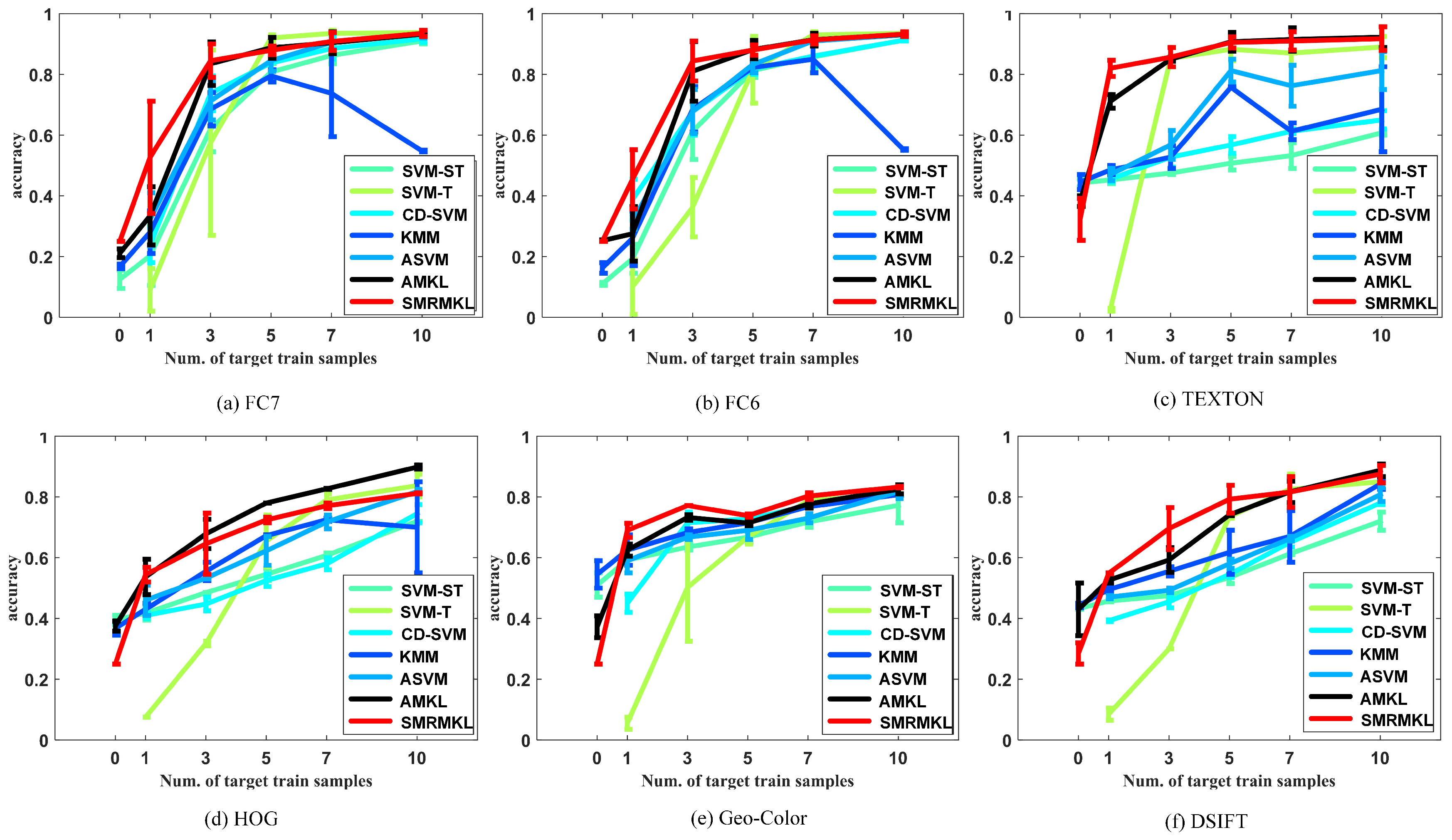
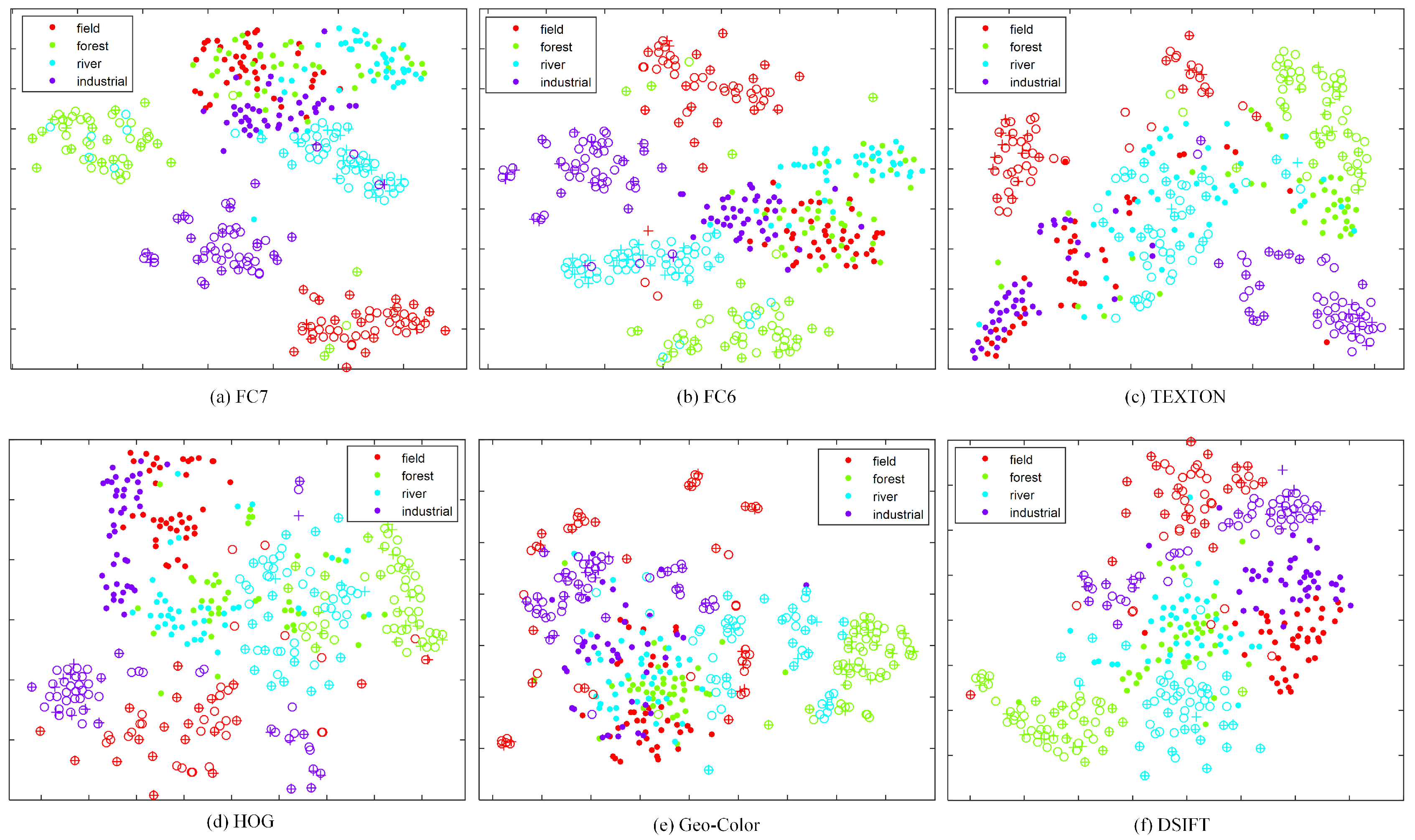
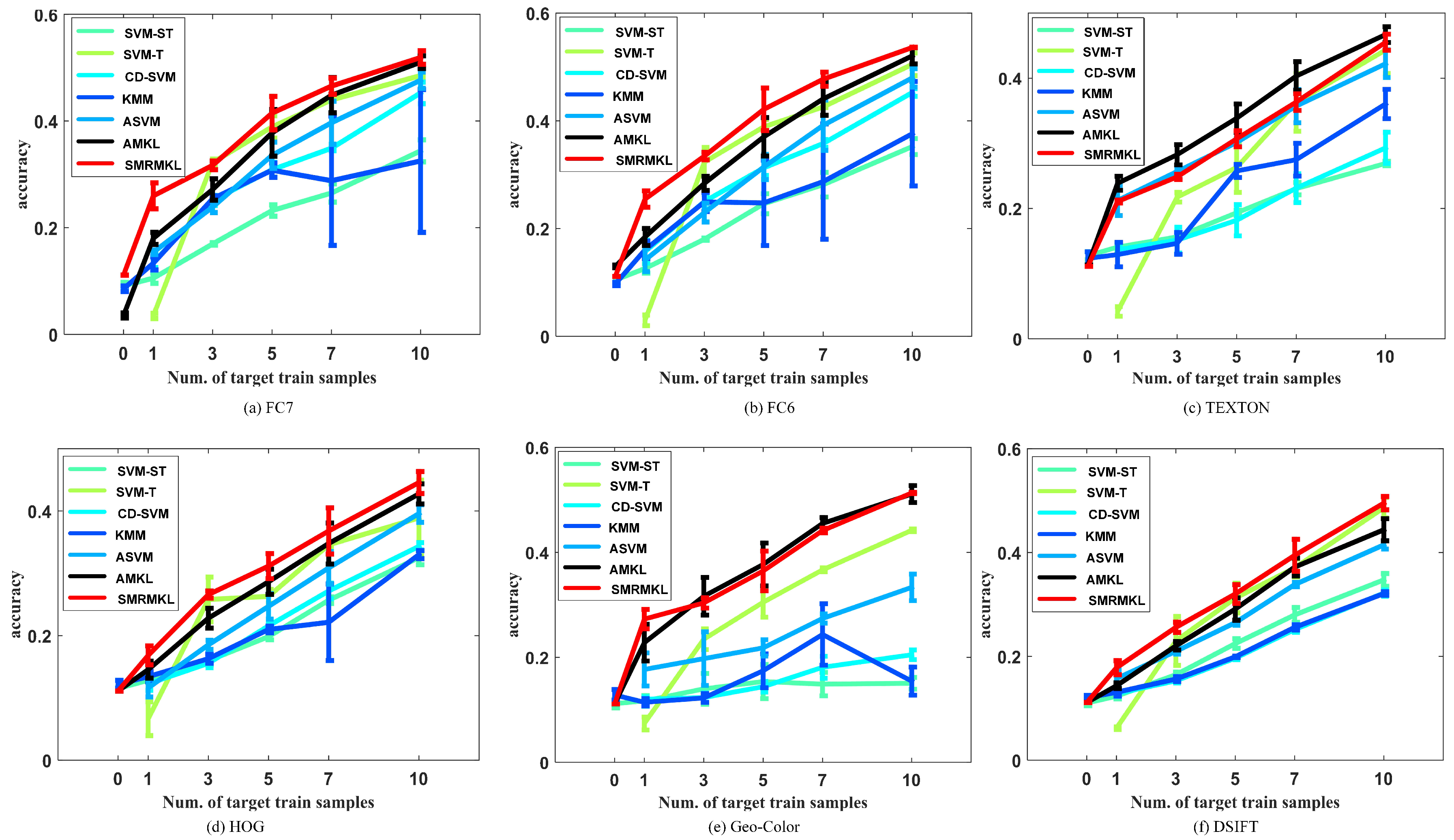
Traditional methods are single feature-based methods; thus, we investigate different approaches on individual features. Figure 6 shows the performance of different approaches with different features for the S1→T3 transfer task in terms of overall accuracy (OA) against the number of target positive training samples. In detail, the curves represent the means of OA and the error bars represent the statistical deviation. The smaller the statistical deviation, the better the consistency of the algorithm. For multiple kernel-based methods, such as A-MKL and SMRMKL, each sub-figure shows the results of single feature with multiple kernels. Figure 7 shows the distributions of S1→T3 cross view scenes with six types of features. Each image’s features in the dataset are projected into two dimensions using t-SNE [33]. The solid points and hollow points represent the source images and target unlabeled images, respectively. In addition, the cross points represent the target labeled images. We observe the following from the results: (1) In most instances, the accuracy curves increase along with the increased number of target labeled training images, which shows that the more information the target domain provides, the better the performance of transfer learning. When the number of target positive training samples exceeds 10, SVM-T has similar performance with other adaptation methods, such as SMRMKL, AMKL and ASVM. (2) A-MKL and SMRMKL lead to better performance than other approaches, which demonstrates the superiority of multiple kernel learning. Compared with A-MKL, SMRMKL achieves higher accuracy in most cases, which demonstrates the successful utilization of unlabeled training images. The exception is the HOG feature in Figure 6d. This observation is not surprising because the differentiation of the HOG feature is worse than the other features’ distributions (as shown in Figure 7d), deteriorating the effect of unlabeled target data in local manifold regularization. (3) The DeCAF and TEXTON features with better differentiation in distribution perform better than the HOG, DSIFT and Geo-Color, which shows that the texture and DeCAF features are more suitable for cross-view transfer tasks.

3.2.2. Analysis on the Kernel Combination Coefficients $d_m$ of the Multiple Features

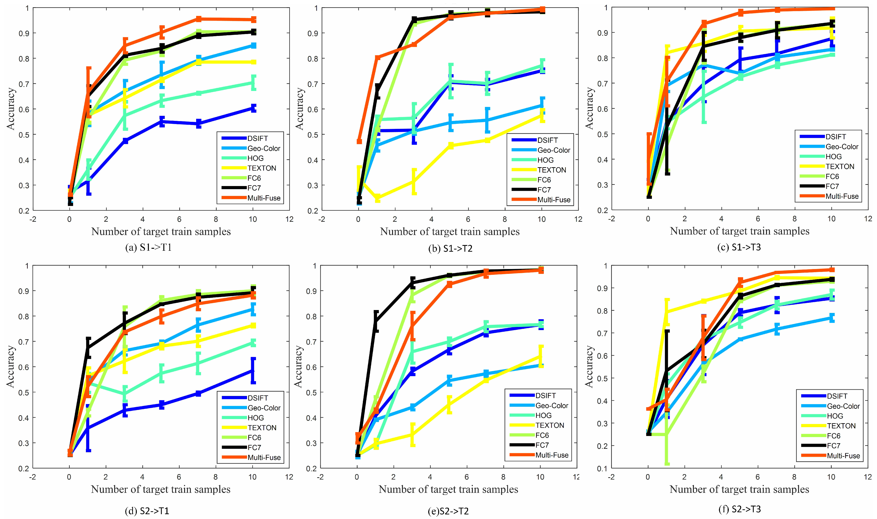
To investigate the performance of multiple kernel learning and the ability to fuse multiple features, we propose two scenarios of cross-view classification with respect to different features and kernels: single-feature with multi-kernels and multi-feature with multi-kernels. Figure 8 shows the performance of SMRMKL for six transfer tasks in terms of classification accuracy against the number of target positive training samples. Multi-Fuse represents the fusion of six features with four types of kernels, and the other features represent the single feature with four types of kernels. From the results, we observe the following: (1) The performance of different features has an obvious dissimilarity in different source-target domain pairs. In most instances, when the number of the target positive training samples exceeds 3, DeCAF features have noticeable improvement over other handcraft features. The results reveal that the DeCAF features generalize well to our cross view datasets. (2) The TEXTON feature has better performance than the DeCAF features for S1→T3 and S2→T3 transfer tasks, whereas it has poor performance for S1→T2 and S2→T2 transfer tasks. This result is possibly caused by the resolution of the image dataset: T3 is a high-resolution satellite scene dataset that has a more similar texture with ground-level datasets. (3) Multi-Fuse generally leads to the highest accuracies in the S1→T1, S1→T2, S1→T3 and S2→T3 transfer tasks. For the S2→T1 and S2→T2 transfer tasks, Multi-Fuse has better performance than four sing hand-craft feature-based methods but slightly worse than single DeCAF feature-based methods. This is possibly caused by the gray-level of S2 dataset and the low-resolution of the T1 and T2 datasets. The results demonstrate that our multiple kernel learning-based approach has the ability to fuse multi-features for improving the performance of cross-view scene classification.

Based on the noticeable improvement of the Multi-Fuse approach, we learned the linear combination coefficient $d_m$ of the multiple features with different types of kernels. The absolute value of each $d_m$ reflects the importance of the corresponding feature and kernel. Taking six types of image features with the Gaussian kernel, we plot the combination coefficient $d_m$ for each class with a fixed number of three target-positive training samples for six pairings of the transfer tasks in

Table 2. The combination coefficients $d_m$ of the multi features with a fixed number of three target positive training samples.

Kernel Coefficients ${\mathit{d}}_{\mathit{m}}$		DSIFT	Geo-Color	HOG	TEXTON	FC6	FC7
S1->T1	agriculture	0.38	0	0.35	0	0.13	0.13
	forest	0.21	0.09	0.19	0	0.24	0.27
	river	0.23	0	0.28	0	0.26	0.23
	industrial	0.34	0	0.39	0	0.13	0.14
S1->T2	agriculture	0.21	0.06	0.36	0	0.17	0.19
	forest	0.07	0.17	0.12	0.16	0.25	0.23
	river	0.23	0.05	0.18	0	0.27	0.27
	industrial	0.33	0.06	0.42	0.02	0.09	0.08
S1->T3	agriculture	0.13	0	0.27	0	0.37	0.23
	forest	0.25	0.06	0.19	0	0.23	0.27
	river	0.16	0.06	0.31	0	0.22	0.25
	industrial	0.29	0.06	0.32	0.03	0.16	0.14
S2->T1	agriculture	0.13	0	0.27	0	0.37	0.23
	forest	0.11	0	0.24	0	0.39	0.26
	river	0.13	0	0.33	0.01	0.37	0.17
	industrial	0.23	0	0.28	0.44	0.05	0
S2->T2	agriculture	0.1	0.07	0.33	0	0.41	0.1
	forest	0.04	0.22	0.22	0	0.42	0.11
	river	0.11	0.02	0.33	0	0.43	0.1
	industrial	0.18	0	0.26	0.52	0.04	0
S2->T3	agriculture	0.03	0.07	0.23	0	0.47	0.2
	forest	0.01	0.34	0.15	0	0.38	0.13
	river	0.04	0	0.32	0	0.45	0.18
	industrial	0.06	0	0.28	0.51	0.15	0

. We observe that the absolute values of DSIFT and HOG are generally larger than other features in S1→T1, S1→T2 and S1→T3 transfer tasks, which shows that DSIFT and HOG play dominant roles among those tasks, whereas the DeCAF features are always larger than other features in the S2→T1,S2→T2 and S2→T3 transfer tasks. This is not surprising because the DSIFT, HOG and DeCAF features are much more distinctive than the Geo-Color and TEXTON features in Figure 7. In Table 2, we also observe that the values of TEXTON are generally close to zero except for the industrial class, which demonstrates that texture is better able to describe the industrial cross-view scene classification.

3.2.3. Effect of Each Regularizer

Our proposed SMRMKL has three components, i.e., multi-kernel minimizing mismatch distribution (MK-MMD) (Section 2.2), structural risk (SR) (Section 2.3), and manifold regularization (MR) (Section 2.4). Here, we investigated the degree of each component’s contribution.

Table 3. The overall accuracy (percent) improvements with different combination of regularization across six pairing of the transfer tasks.

Overall Accuracy	S1->T1	S1->T2	S1->T3	S2->T1	S2->T2	S2->T3
SR+MK-MMD	70.65	81.04	81.00	75.18	90.04	65.08
SR+MR	50.89	62.19	61.25	54.11	63.94	61.63
SR+MK-MMD+MR	81.19	95.21	84.50	77.14	93.08	65.27

shows the performance improvements on different combinations of regularizers (i.e., SR+MK-MMD, SR+MR, and SR+MK-MMD+MR) with a fixed number of three target-positive training samples. The results indicate that SR+MK-MMD+MR exhibits a higher accuracy than SR+MK-MMD and SR+MR, which demonstrates that the combination of three regularizers can effectively improve the adaptation performance. Furthermore, SR+MK-MMD leads to a better performance than SR+MR, which means that the MK-MMD regularizer has a higher contribution than the MR regularizer.

3.2.4. Analysis on Parameters

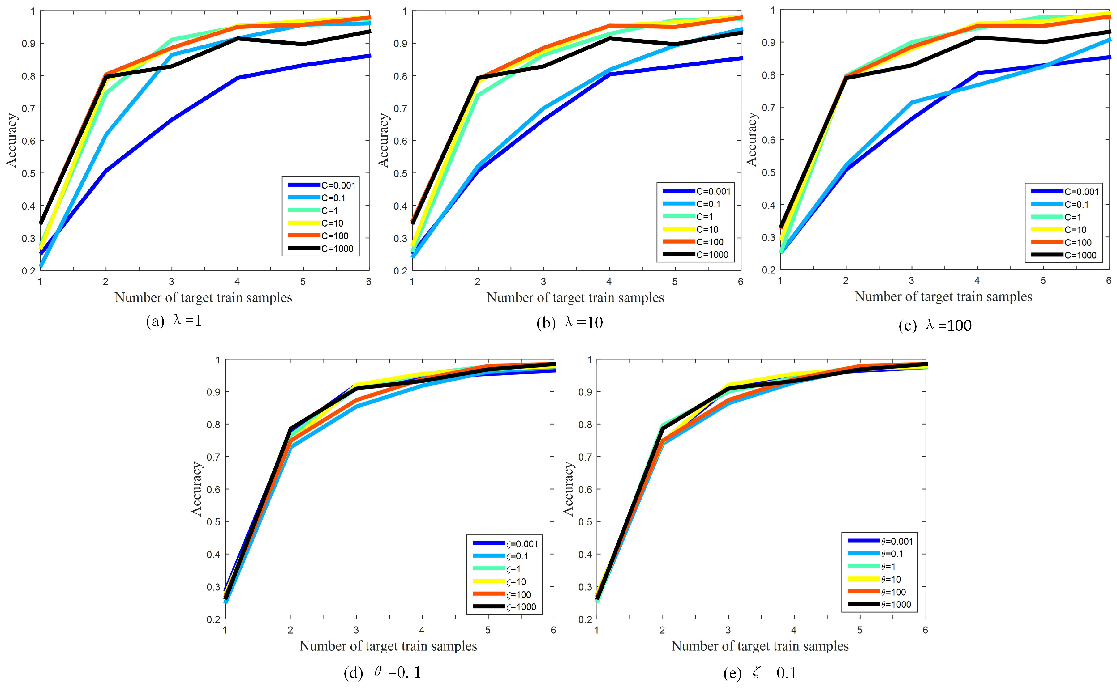
To investigate the impact of each parameter, the regularization parameter C and three trade-off parameters $\theta$, $\lambda$, $\zeta$ are taken into consideration. In Figure 9a–c, we show the impact of regularization parameter C and trade-off parameters $\lambda$ when they are set to take different values of the S1→T1 transfer task. From the results, we can see that C has a dominant impact on classification accuracy, whereas $\lambda$ is not considerably sensitive to the performance. Thus, we empirically set $C=100$ and $\lambda =10$ in our subsequent evaluations. In Figure 9d,e, we show the impact of trade-off parameters $\theta$ and $\zeta$ with different values for the S1→T1 transfer task. From the results, we can see that the performance of our method is not sensitive to trade-off parameters $\theta$ and $\zeta$.

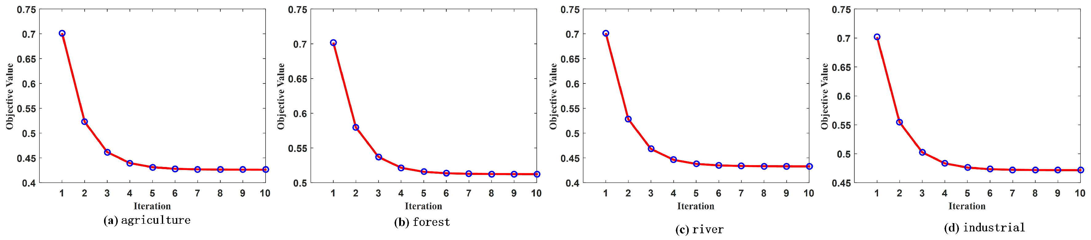
Recall that we iteratively update the linear combination coefficient $d_m$ and dual variable $\alpha$ in SMRMKL (see Section 2.5). We discuss the convergence of the iterative algorithm of SMRMKL. Taking S2→T1 transfer task, we draw the change of the objective value for each class with respect to the number of iterations in Figure 10. We observe that SMRMKL converges after about six iterations for all categories. Other transfer tasks also have similar observations.

3.3. Aerial-to-Satellite Transfer

To demonstrate the robustness of our method, we evaluated the performance of our method in transferring scene models from aerial scenes to satellite scenes. Figure 11 further details the performance of different approaches with different features for the aerial-to-satellite transfer task in terms of classification accuracy against the number of target-positive training samples. In this figure, SMRMKL successfully brings up the performance of different features, which demonstrates that SMRMKL is significantly better than other approaches to the aerial-to-satellite transfer task. The exception is the TEXTON feature in Figure 11c. This observation may be the result of the differentiation of the TEXTON feature deteriorating the effect of unlabeled target data in local manifold regularization, which deteriorates the adaptation performance.

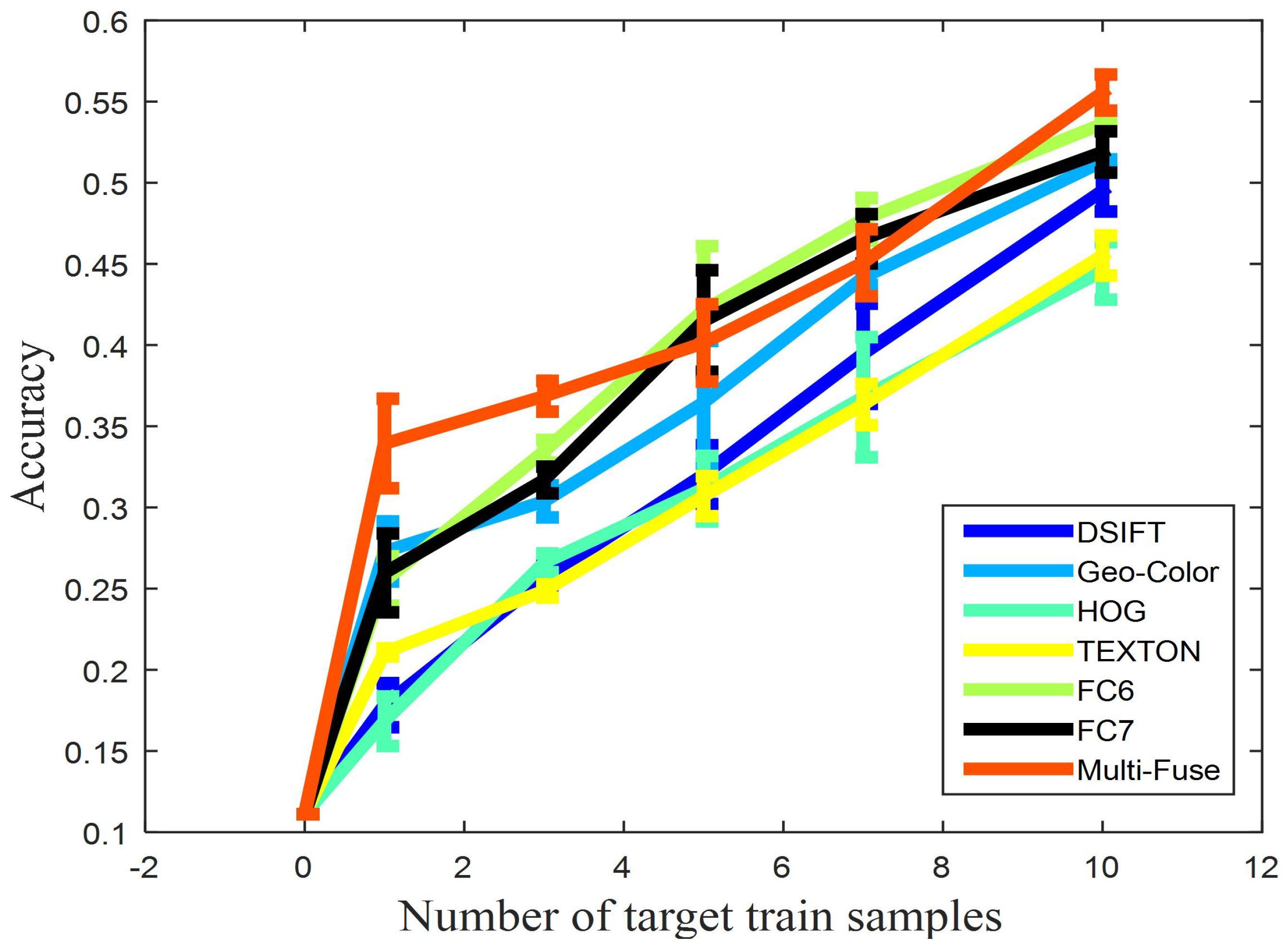
Figure 12 shows the performance of SMRMKL with different features for the aerial-to-satellite transfer task in terms of classification accuracy against the number of target positive training samples. From the results, we can see that DeCAF features have noticeable improvement over other handcraft features. Geo-Color has better performance than other three hand-craft features. In addition, Multi-Fuse generally leads to the highest accuracies in this transfer task. The result indicates that our multiple kernel learning-based approach has the ability to fuse multi-features to improve the performance of aerial-to-satellite scene classification. Furthermore, we can observe that the classification accuracy is very low without using samples form the target domain (i.e., the number of target train samples is 0). As the number of target training samples increases, the classification accuracy increases significantly. As can be seen in Figure 11 and Figure 12, the curve does not have a gentle trend. This proves that the participation of target domain training samples is very important for improving the classification accuracy. However, due to the small size of aerial-to-satellite scene dataset, up to 10 samples per class from the target domain participated in the training. This will result in limited classification accuracy. In our future work, we will collect more samples for training. We believe that the classification accuracy will be improved.

To further observe the performance in individual categories, the mean Average Precision (mAP) of different features with respect to each class is drawn in

Table 4. Per-class mAPs of different features with 10 target positive examples for all nine categories.

mAPs	DSIFT	Geo-Color	HOG	TEXTON	FC6	FC7	Multi-Fuse
residential	0.42	0.46	0.44	0.47	0.48	0.5	0.42
parking	0.47	0.37	0.45	0.61	0.5	0.48	0.5
harbor	0.5	0.51	0.49	0.5	0.57	0.56	0.51
industry	0.44	0.39	0.41	0.51	0.47	0.46	0.46
farmland	0.66	0.63	0.63	0.56	0.67	0.65	0.72
viaduct	0.42	0.44	0.44	0.49	0.46	0.45	0.53
river	0.55	0.51	0.45	0.44	0.57	0.52	0.57
forest	0.76	0.71	0.77	0.78	0.81	0.79	0.84
beach	0.86	0.86	0.68	0.81	0.94	0.93	0.93

. The corresponding confusion matrices are shown in

Table 5. The confusion matrices of Multi-Fuse based SMRMKL with 10 target positive examples per class for aerial-to-satellite classification. The overall accuracy is 56.79% and the Kappa is 0.5139.

Class	Residential	Parking	Harbor	Industry	Farmland	Viaduct	River	Forest	Beach	Total	User. Acc (%)
residential	18	16	11	0	0	0	0	0	0	45	29.51
parking	9	30	4	1	0	0	1	0	0	45	56.6
harbor	16	6	19	1	0	0	1	2	0	45	51.35
industry	10	1	3	14	16	1	0	0	0	45	70.00
farmland	0	0	0	4	39	2	0	0	0	45	61.9
viaduct	0	0	0	0	8	20	17	0	0	45	60.61
river	0	0	0	0	0	10	24	9	2	45	55.81
forest	0	0	0	0	0	0	0	32	13	45	69.57
beach	8	0	0	0	0	0	0	3	34	45	69.39
Total	61	53	37	20	63	33	43	46	49	405
Prod. Acc (%)	40.00	66.67	42.22	31.11	86.67	44.44	53.33	71.11	75.56

. We can observe that different feature responds differently to each class. For instance, “parking” and “industry” are better classified with TEXTON, and “residential” and “harbor” show better results with DeCAF features. For the last five categories, Multi-Fuse-based SMRMKL successfully improves the mAP performance. In Table 5, we can see that most of the scene categories could be correctly classified except “residential”, “harbor”, “industry”, “river”, and “beach”, whose visual aspects are significantly different between the aerial images and satellite images. In addition, “residential” and “harbor” from the aerial images are easily confused with “parking” and “industry” from the satellite images due to the similar configuration in Figure 5. It is also difficult to distinguish “viaduct” and “river” due to the similar winding attribute.

3.4. Running Time and Memory Usage

In the following, the computational complexity of SMRMKL in Algorithm 1 is investigated. Here, we suppose multiple types of features are pre-computed before SMRMKL training. Then, the computational cost for the calculation of the kernel matrix K in Step 1 and $\tilde{K}$ in Step 3 takes the same time $O(M{N}^2)$, where M is the number of base kernels and N is the number of training images in the source and target domains. Suppose the mean computational cost for the two-class classification takes the time $O(D^2{N}^2)$, where D is the dimensionality of each feature. Then, the computational cost of Step 3 is $O(J(k{D}^2{N}^2+M{N}^2))$, where k is the number of required iterations for convergence and J is the number of categories. For Memory Usage, taking six types of image features with four kind of kernels, the kernel matrix of the small size transfer tasks (i.e., S1→T1, S1→T2 and S1→T3) occupies 40.6 megabytes on average, while the kernel matrix of the large size transfer tasks (i.e., S2→T1, S2→T2 and S2→T3) occupies 348.5 megabytes on average. When the kernel matrixes are pre-computed, our algorithm is still effective in computation.

4. Conclusions

In this paper, we propose transferring scene models from ground-view images to very high-resolution remote sensing images. Specifically, a semi-supervised manifold-regularized multiple kernel learning (SMRMKL) algorithm that jointly minimizes the mismatch of distributions between the two domains and leverages available unlabeled target samples to capture the local structure in the target domain is presented. In addition, we conduct an in-depth investigation on various aspects of SMRMKL, such as analysis on the effect of each regularizer, the combination coefficients on the multiple kernels, and the convergence of the learning algorithm. Extensive experimental results on both cross-view and aerial-to-satellite scene datasets show that: (1) SMRMKL has an appealing extension ability to effectively fuse different types of visual features and improve the classification accuracy, whereas traditional methods focus on one kind of features. In addition, SMRMKL could indicate which type of feature plays dominant roles among scene transfer tasks, this is important for feature selection. (2) In the past, most cross-view scene model adaptation models are unsupervised methods [28,29,30]. Without using target domain samples, the classification accuracy is limited. SMRMKL is semi-supervised method which proves that the participation of target domain training samples is very important for improving the adaptation classification accuracy. (3) Manifold regularization can improve the adaptation performance by utilizing unlabeled target samples. In practical applications, there are many unlabeled samples. How to effectively leverage these unlabeled samples has important application significance. However, the results in our manuscript are still limited in practical applications. The dataset constructed is simple. The number of samples in the dataset is small. In our future work, we will extend this work to a larger cross-view dataset collected from web images and UAV( unmanned aerial vehicle) images. Furthermore, our work is expected to be applied to the visual attributes adaptation. Visual attributes can be considered as a middle-level semantic cue that bridges the gap between low-level image features and high-level object classes. Thus, visual attributes have the advantage of transcending specific semantic categories or describing scene images across categories.

References

- Cheng, G.; Han, J.; Lu, X. Remote Sensing Image Scene Classification: Benchmark and State of the Art. Proc. IEEE 2017, 105, 1865–1883. [Google Scholar] [CrossRef]
- Qiu, S.; Wen, G.; Liu, J.; Deng, Z.; Fan, Y. Unified Partial Configuration Model Framework for Fast Partially Occluded Object Detection in High-Resolution Remote Sensing Images. Remote Sens. 2018, 10, 464. [Google Scholar] [CrossRef]
- Tang, T.; Zhou, S.; Deng, Z.; Lei, L.; Zou, H. Arbitrary-Oriented Vehicle Detection in Aerial Imagery with Single Convolutional Neural Networks. Remote Sens. 2017, 9, 1170. [Google Scholar] [CrossRef]
- Luo, Y.M.; Ouyang, Y.; Zhang, R.C.; Feng, H.M. Multi-Feature Joint Sparse Model for the Classification of Mangrove Remote Sensing Images. Int. J. Geo-Inf. 2017, 6, 177. [Google Scholar] [CrossRef]
- He, C.; Liu, X.; Kang, C.; Chen, D.; Liao, M. Attribute Learning for SAR Image Classification. Int. J. Geo-Inf. 2017, 6, 111. [Google Scholar] [CrossRef]
- Hu, F.; Xia, G.S.; Hu, J.; Zhong, Y.; Xu, K. Fast Binary Coding for the Scene Classification of High-Resolution Remote Sensing Imagery. Remote Sens. 2016, 8, 555. [Google Scholar] [CrossRef]
- Chen, C. Remote Sensing Image Scene Classification Using Multi-scale Completed Local Binary Patterns and Fisher Vectors. Remote Sens. 2016, 8, 483. [Google Scholar] [CrossRef]
- Yu, H.; Yang, W.; Xia, G.S.; Liu, G. A Color-Texture-Structure Descriptor for High-Resolution Satellite Image Classification. Remote Sens. 2016, 8, 259. [Google Scholar] [CrossRef]
- Hu, F.; Xia, G.S.; Hu, J.; Zhang, L. Transferring Deep Convolutional Neural Networks for the Scene Classification of High-Resolution Remote Sensing Imagery. Remote Sens. 2015, 7, 14680–14707. [Google Scholar] [CrossRef]
- Liu, N.; Lu, X.; Wan, L.; Huo, H.; Fang, T. Improving the Separability of Deep Features with Discriminative Convolution Filters for RSI Classification. Int. J. Geo-Inf. 2018, 7, 95. [Google Scholar] [CrossRef]
- Wang, J.; Luo, C.; Huang, H.; Zhao, H.; Wang, S. Transferring Pre-Trained Deep CNNs for Remote Scene Classification with General Features Learned from Linear PCA Network. Remote Sens. 2017, 9, 225. [Google Scholar] [CrossRef]
- Ding, C.; Li, Y.; Xia, Y.; Wei, W.; Zhang, L.; Zhang, Y. Convolutional Neural Networks Based Hyperspectral Image Classification Method with Adaptive Kernels. Remote Sens. 2017, 9, 618. [Google Scholar] [CrossRef]
- Han, X.; Zhong, Y.; Cao, L.; Zhang, L. Pre-Trained AlexNet Architecture with Pyramid Pooling and Supervision for High Spatial Resolution Remote Sensing Image Scene Classification. Remote Sens. 2017, 9, 848. [Google Scholar] [CrossRef]
- Qi, K.; Yang, C.; Guan, Q.; Wu, H.; Gong, J. A Multiscale Deeply Described Correlatons-Based Model for Land-Use Scene Classification. Remote Sens. 2017, 9, 917. [Google Scholar] [CrossRef]
- Gong, X.; Xie, Z.; Liu, Y.; Shi, X.; Zheng, Z. Deep Salient Feature Based Anti-Noise Transfer Network for Scene Classification of Remote Sensing Imagery. Remote Sens. 2018, 10, 410. [Google Scholar] [CrossRef]
- Liu, Y.; Huang, C. Scene Classification via Triplet Networks. IEEE J. Sel. Top. Appl. Earth Obs. Remote Sens. 2018, 11, 220–237. [Google Scholar] [CrossRef]
- Deng, Z.; Sun, H.; Zhou, S.; Zhao, J.; Lei, L.; Zou, H. Multi-scale object detection in remote sensing imagery with convolutional neural networks. ISPRS J. Photogram. Remote Sens. 2018. [Google Scholar] [CrossRef]
- Deng, Z.; Sun, H.; Zhou, S.; Zhao, J.; Zou, H. Toward Fast and Accurate Vehicle Detection in Aerial Images Using Coupled Region-Based Convolutional Neural Networks. IEEE J. Sel. Top. Appl. Earth Obs. Remote Sens. 2017, 10, 3652–3664. [Google Scholar] [CrossRef]
- Tuia, D.; Persello, C.; Bruzzone, L. Domain Adaptation for the Classification of Remote Sensing Data: An Overview of Recent Advances. IEEE Geosci. Remote Sens. Mag. 2016, 4, 41–57. [Google Scholar] [CrossRef]
- Persello, C.; Bruzzone, L. Kernel-Based Domain-Invariant Feature Selection in Hyperspectral Images for Transfer Learning. IEEE Trans. Geosci. Remote Sens. 2015, 54, 1–12. [Google Scholar] [CrossRef]
- Yang, H.L.; Crawford, M.M. Domain Adaptation With Preservation of Manifold Geometry for Hyperspectral Image Classification. IEEE J. Sel. Top. Appl. Earth Obs. Remote Sens. 2016, 9, 543–555. [Google Scholar] [CrossRef]
- Othman, E.; Bazi, Y.; Alajlan, N.; Alhichri, H. Three-Layer Convex Network for Domain Adaptation in Multitemporal VHR Images. IEEE Geosci. Remote Sens. Lett. 2016, 13, 354–358. [Google Scholar] [CrossRef]
- Li, X.; Zhang, L.; Du, B.; Zhang, L.; Shi, Q. Iterative Reweighting Heterogeneous Transfer Learning Framework for Supervised Remote Sensing Image Classification. IEEE J. Sel. Top. Appl. Earth Obs. Remote Sens. 2017, 10, 2022–2035. [Google Scholar] [CrossRef]
- Wang, X.; Huang, W.; Cheng, Y.; Yu, Q.; Wei, Z. Multisource Domain Attribute Adaptation Based on Adaptive Multikernel Alignment Learning. IEEE Trans. Syst. Man Cybern. Syst. 2018, 1–12. [Google Scholar] [CrossRef]
- Deng, J.; Dong, W.; Socher, R.; Li, L.J.; Li, K.; Li, F.F. ImageNet: A large-scale hierarchical image database. In Proceedings of the 2009 IEEE Conference on Computer Vision and Pattern Recognition (2009), Miami, FL, USA, 20–25 June 2009; pp. 248–255. [Google Scholar]
- Patterson, G.; Xu, C.; Su, H.; Hays, J. The SUN Attribute Database: Beyond Categories for Deeper Scene Understanding. Int. J. Comput. Vis. 2014, 108, 59–81. [Google Scholar] [CrossRef]
- Workman, S.; Souvenir, R.; Jacobs, N. Wide-Area Image Geolocalization with Aerial Reference Imagery. In Proceedings of the 2015 IEEE International Conference on Computer Vision (ICCV), Santiago, Chile, 7–13 December 2015. [Google Scholar]
- Sun, H.; Liu, S.; Zhou, S.; Zou, H. Transfer Sparse Subspace Analysis for Unsupervised Cross-View Scene Model Adaptation. IEEE J. Sel. Top. Appl. Earth Obs. Remote Sens. 2016, 9, 2901–2909. [Google Scholar] [CrossRef]
- Sun, H.; Liu, S.; Zhou, S.; Zou, H. Unsupervised Cross-View Semantic Transfer for Remote Sensing Image Classification. IEEE Geosci. Remote Sens. Lett. 2016, 13, 13–17. [Google Scholar] [CrossRef]
- Sun, H.; Liu, S.; Zhou, S. Discriminative Subspace Alignment for Unsupervised Visual Domain Adaptation. Neural Process. Lett. 2016, 44, 1–15. [Google Scholar] [CrossRef]
- Sun, H.; Deng, Z.; Liu, S.; Zhou, S. Transferring ground level image annotations to aerial and satellite scenes by discriminative subspace alignment. In Proceedings of the Geoscience and Remote Sensing Symposium, Beijing, China, 10–15 July 2016; pp. 2292–2295. [Google Scholar]
- Deng, Z.; Sun, H.; Zhou, S.; Ji, K. Semi-supervised cross-view scene model adaptation for remote sensing image classification. In Proceedings of the Geoscience and Remote Sensing Symposium, Beijing, China, 10–15 July 2016; pp. 2376–2379. [Google Scholar]
- Laurens, V.; Der, M.; Hinton, G. Viualizing data using t-SNE. J. Mach. Learn. Res. 2008, 9, 2579–2605. [Google Scholar]
- Patel, V.M.; Gopalan, R.; Li, R.; Chellappa, R. Visual domain adaptation: A survey of recent advances. IEEE Signal Process. Mag. 2015, 32, 53–69. [Google Scholar] [CrossRef]
- Volpi, M.; Camps-Valls, G.; Tuia, D. Spectral alignment of multi-temporal cross-sensor images with automated kernel canonical correlation analysis. J. Photogramm. Remote Sens. 2015, 23, 167–169. [Google Scholar] [CrossRef]
- Long, M.; Wang, J.; Jordan, M.I. Unsupervised Domain Adaptation with Residual Transfer Networks. arXiv, 2016; arXiv:1602.04433. [Google Scholar]
- Long, M.; Wang, J.; Cao, Y.; Sun, J. Deep Learning of Transferable Representation for Scalable Domain Adaptation. IEEE Trans. Knowl. Data Eng. 2016, 28, 2027–2040. [Google Scholar] [CrossRef]
- Gueguen, L. Classifying Compound Structures in Satellite Images: A Compressed Representation for Fast Queries. IEEE Trans. Geosci. Remote Sens. 2015, 53, 1803–1818. [Google Scholar] [CrossRef]
- Duan, L.; Xu, D.; Tsang, I.W.; Luo, J. Visual event recognition in videos by learning from Web data. Patten Anal. Mach. Intell. IEEE Trans. 2012, 34, 1667–1680. [Google Scholar] [CrossRef] [PubMed]
- Long, M.; Cao, Y.; Wang, J.; Jordan, M.I. Learning Transferable Features with Deep Adaptation Networks. arXiv, 2015; arXiv:1502.02791. [Google Scholar]
- Melacci, S.; Belkin, M. Laplacian Support Vector Machines Trained in the Primal. J. Mach. Learn. Res. 2009, 12, 1149–1184. [Google Scholar]
- Belkin, M.; Niyogi, P.; Sindhwani, V. Manifold Regularization: A Geometric Framework for Learning from Labeled and Unlabeled Examples. J. Mach. Learn. Res. 2006, 7, 2399–2434. [Google Scholar]
- Chang, C.C.; Lin, C.J. LIBSVM: A library for support vector machines. Acm Trans. Intell. Syst. Technol. 2011, 2, 389–396. [Google Scholar] [CrossRef]
- Rakotomamonjy, A.; Bach, F.R.; Canu, S.; Grandvalet, Y. Simplemkl. J. Mach. Learn. Res. 2008, 9, 2491–2521. [Google Scholar]
- Risojevic, V.; Babic, Z. Aerial image classification using structural texture similarity. In Proceedings of the 2011 IEEE International Symposium on Signal Processing and Information Technology (ISSPIT), Bilbao, Spain, 14–17 Decemner 2011; pp. 190–195. [Google Scholar]
- Yang, Y.; Newsam, S. Bag-of-visual-words and spatial extensions for land-use classification. In Proceedings of the ACM Sigspatial International Symposium on Advances in Geographic Information Systems, Acm-Gis 2010, San Jose, CA, USA, 3–5 November 2010; pp. 270–279. [Google Scholar]
- Dai, D.; Yang, W. Satellite Image Classification via Two-Layer Sparse Coding With Biased Image Representation. IEEE Geosci. Remote Sens. Lett. 2011, 8, 173–176. [Google Scholar] [CrossRef]
- Kataoka, H.; Iwata, K.; Satoh, Y. Decaf: A deep convolutional activation feature for generic visual recognition. Comput. Sci. 2013, 50, 815–830. [Google Scholar]
- Yang, J.; Yan, R.; Hauptmann, A.G. Cross-domain video concept detection using adaptive svms. In Proceedings of the 2007 International Conference on Multimedia, Augsburg, Germany, 25–29 September 2007; pp. 188–197. [Google Scholar]
- Jiang, W.; Zavesky, E.; Chang, S.F.; Loui, A. Cross-Domain Learning Methods for High-Level Visual Concept Classification. In Proceedings of the 15th IEEE International Conference on Image, San Diego, CA, USA, 12–15 October 2008; pp. 161–164. [Google Scholar]
- Duan, L.; Tsang, I.W.; Xu, D. Domain transfer multiple kernel learning. IEEE Trans. Patten Anal. Mach. Intell. 2011, 34, 465–479. [Google Scholar] [CrossRef] [PubMed]
Figure 1.
Ground-to-overhead view and aerial-to-satellite scene transfer task.
Figure 2.
The flowchart of semi-supervised manifold-regularized multiple kernel learning.
Figure 3.
Illustration of multiple kernel learning and manifold regularization.
Figure 4.
Samples of our cross-view datasets.
Figure 5.
Nine common categories of satellite scenes from WHU-RS19 dataset (top row) and aerial scenes from UC Merced dataset (bottom row): (1) residential; (2) parking lot; (3) port/harbor; (4) industry/building; (5) farmland/ agriculture; (6) viaduct/ overpass; (7) river; (8) forest; and (9) beach.
Figure 6.
The performance (means and standard deviation of overall accuracy) of different approaches with different features for S1→T3 transfer task.
Figure 7.
2D visualization of the S1→T3 cross-view scene dataset with different features. The solid points, hollow points, and cross points represent the source images, target unlabeled images and target labeled images, respectively.
Figure 8.
The performance (means and standard deviation of overall accuracy) of our approach with different features for six transfer tasks.
Figure 9.
The performance (classification accuracy) of Multi-Fuse based SMRMKL for S1→T1 transfer task with different trade-off parameters.
Figure 10.
Illustration of the convergence of the SMRMKL learning algorithm for four categories.
Figure 11.
The performance (mean and standard deviation of overall accuracy) of different approaches using different features with respect to different numbers of target samples per class for the aerial-to-satellite transfer task.
Figure 12.
The performance (mean and standard deviation of overall accuracy) of our approach using different features with respect to different numbers of target samples per class for the aerial-to-satellite transfer task.