Spatial Modelling and Prediction Assessment of Soil Iron Using Kriging Interpolation with pH as Auxiliary Information

Abstract

In this study, different interpolation techniques are presented, assessed, and compared for the estimation of soil iron (Fe) contents in locations where observations were not available. Initially, 400 soil samples from the Kozani area, which is near Polifitou Lake in northern Greece, were randomly collected from 2013 to 2015 and were analysed in the laboratory to determine the soil Fe concentrations and pH. The soil Fe concentrations were examined for spatial autocorrelation, and semivariograms were used to determine whether pH and Fe exhibited spatial cross correlation. Three interpolation methods, including Ordinary Kriging, Universal Kriging, and Co-Kriging, were applied, and their results were compared with the use of two different cross-validation methods. In the current study, there was evidence of spatial cross correlation of soil Fe and pH for each year, which was subsequently used to improve the interpolation results in locations where there were no measurements. In nearly all cases, Co-Kriging, which takes advantage of the covariance between the two regionalized variables (Fe and pH), outperformed the other interpolation techniques each year.

1. Introduction

Iron (Fe) is as important for plant nutrition as the major (N, P, K) and secondary (Ca, Mg) nutrients. In fact, iron is so important to plants that they have developed a system to release ions into the soil to lower the pH to prevent iron from becoming unavailable [1]. Iron deficiencies generally result more from interference issues from other ions than from low levels of iron in the soil. A small amount of bicarbonates present in the soil, for example, can block uptake and induce iron deficiency [2], something that is usually found in soils with an alkaline pH level of more than 7. Therefore, at high pH levels, there is an essential factor inducing iron deficiencies.

Measuring soil parameters exhaustively in wide areas is a time consuming and costly effort. However, by using geostatistical analysis, specifically spatial interpolation techniques, the predicted values of soil parameters can be estimated in locations where observations are not available [3,4,5].

Geostatistics is defined as a branch of statistics that specializes in the analysis and interpretation of any spatially referenced data [6] and involves the estimation and modelling of spatial correlation [7]. Its strength is that it recognizes spatial variability at both the large scale and the small scale and models both spatial trends and spatial correlation [8]. However, among the available multiple geostatistical models and techniques, the appropriate models and techniques that will give the most accurate and unbiased results for each case should be chosen.

Geostatistics are extensively used in environmental sciences [6,9,10,11]. Specifically, in soil science, correlations between multiple soil properties [12] and the prediction of soil heavy metal contents [13] across Europe have been thoroughly studied. In precision agriculture (large scales), different techniques are also used to improve the accuracy of mapping soil variables when using electrical conductivity [14] or when predicting soil parameters such as nitrogen (N) with elevation data as auxiliary information [15]. Geostatistics, remote sensing (e.g., ASTER, Landsat images) and the use of auxiliary maps (Digital Elevation Models, soil maps, land coverage maps, etc.) have also been extensively studied [16,17,18,19,20,21].

The objective of this study was to compare geostatistical techniques using the soil Fe and pH data from the 400 soil samples in northern Greece from 2013 to 2015. Although soil Fe and pH are correlated according to the bibliographies of [22,23], their spatial distribution and spatial cross-correlation have not been extensively studied.

In the current study, the three more common techniques among the different spatial interpolation techniques [8,9,24,25] were used for predicting soil iron, and their results were assessed. These techniques included Ordinary Kriging (OK), Universal Kriging (UK), and, finally, Co-Kriging (Co-Kr), which tries to utilize the possible spatial cross-correlation between variables (here, soil Fe and pH).

To determine the true prediction accuracy of the prediction models that were used (the three interpolations), cross-validation [26,27] was performed using two different methods. Initially, an independent data set (holdout method) was used, and then, subsequently, the leave-one-out method (LOOCV) was used. The performances of the different interpolation methods were assessed by the differences between the observations and predictions at validation sites and expressed as the mean error (ME), root mean square error (RMSE), and mean squared deviation ratio (MSDR).

2. Materials and Methods

2.1. Study Area

A soil survey was conducted in the regional unit of Kozani in northern Greece. The specific area is located next to Polifitou Lake (Figure 1) at an altitude of approximately 400 m above sea level (from 300 m in areas close to the lake to 500 m) and covers an area of approximately 28 km².

The area extends from latitudes of 40°11′19.07″ N to 40°17′21.71″ N and from longitudes of 21°59′20.94″ E to 22°6′9.17″ E in WGS84. The main agricultural crops are peach and nectarine trees.

2.2. Soil Sampling and Laboratory Analysis

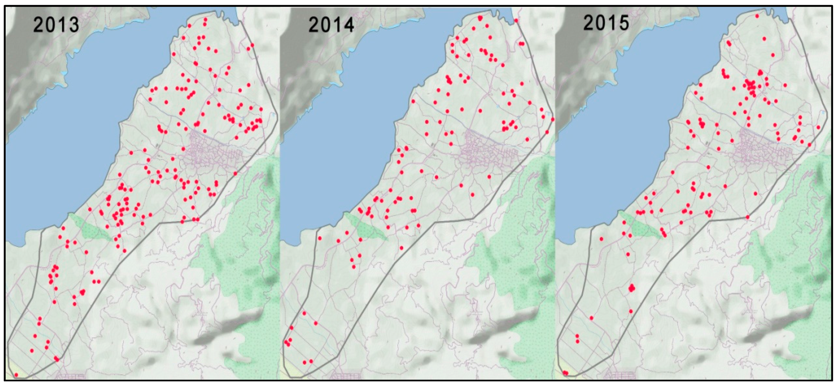
During this soil survey, 400 field parcels were randomly sampled from 2013 to 2015 so that different parts of the cultivated area would be covered. Specifically, 177, 109, and 114 soil samples were taken in 2013, 2014, and 2015, respectively, accounting for 400 samples for all three years (Figure 2). Global Positioning System (GPS) receivers were used to identify the sampling positions. Soil sampling took place during the period from autumn to winter for the three consecutive years.

In more detail, during the soil sampling procedure, a composite soil sample comprised of several sub-samples obtained to a depth of 30 cm was obtained from each field parcel. The soil samples were dried in the Soil Science Institute lab and analysed for pH and iron (Fe). The pH was measured from a saturated soil paste, and Fe was extracted using diethylenetriaminepentaacetic acid (DTPA) and measured using inductively coupled plasma optical emission spectrometry (ICP-OES).

2.3. Semivariograms and Semivariogram Modelling

To apply geostatistics and specifically interpolation methods, we first estimated the experimental variograms (semivariogram) of our Fe and pH data, the cross-semivariogram between them, and their fitted models for every year.

The semivariance [24] quantifies the spatial variation in a variable, as seen in Equation (1):

$$\gamma \left(h\right)=\frac{1}{2N\left(h\right)}{\displaystyle \sum }_i^{N\left(h\right)}{\left[Z\left(s_i\right)-Z\left(s_i+h\right)\right]}^2$$

(1)

where $s_i$ are the locations of the samples, $Z\left(s_i\right)$ is their values, h is the separate distance between the $Z\left(s_i\right)$ and $Z\left(s_i+h\right)$ locations, and $N\left(h\right)$ is the number of pairs $Z\left(s_i\right)$ over the separated distance h. The plot of the estimated $\gamma \left(h\right)$ values against h is called a semivariogram.

Key parameters of the semivariogram are the ‘nugget’ (C₀), which represents measurement errors and the short distance unexplained or random spatial variation; the total ‘sill’ (C₀ + C₁), which is the semivariance value at which the semivariogram levels off and represents the variance of the variable; and, finally, the ‘range’ (a), which is the value of distance at which the semivariogram reaches the sill and, beyond that, distance at which the data are no longer correlated. The semivariogram and its parameters can only be positive.

The spatial dependence of the variables in the semivariograms can be assessed by estimating the nugget to the total sill ratio (C₀/C₀ + C₁). A ratio less than 25% indicates strong spatial dependence, a ratio between 25% and 75% indicates a moderate spatial dependence, and a ratio over 75% indicates a weak spatial dependence [28].

In applied geostatistics, experimental semivariograms are approximated by model functions (the semivariograms models) [3,29]. Some common simple models are the nugget, exponential, spherical, and linear models [8,30]. The model that more often describes the reality in soil [5] is the spherical model based on the following equation:

$$\begin{gathered} \gamma \left(h\right)=C_0+C_1\left[\frac{3}{2}\left(\frac{h}{a}\right)-\frac{1}{2}{\left(\frac{h}{a}\right)}^3\right]whenh\le a \\ =C_0+C_{1}whenh\ge a \\ =C_{0}whenh=0 \end{gathered}$$

(2)

where C₀ is the nugget, α the range, and C₀ + C₁ is the sill. Semivariogram modelling and estimation is extremely important for structural analysis and spatial interpolation [31].

2.4. Kriging Interpolation

Kriging is an exact interpolator that gives the best unbiased linear estimates of point values. Having measured N data values, Z($s_1$), Z($s_2$), ..., Z($s_N$) at $s_1$, $s_2$, ..., $s_N$ locations, we estimate the $\widehat{Z}\left(s_0\right)$ at the unknown location of s₀ with the following equation:

$$\widehat{Z}\left(s_0\right)={\displaystyle \sum }_{i=1}^N{\lambda }_{i}Z\left(s_i\right)$$

(3)

where $Z\left(s_i\right)$ is the measured value at the $s_i$ location and ${\lambda }_i$ is the unknown weight for the measured value at the $s_i$ location. The goal of this process is to determine the weights λ_i that minimize the variance of the estimator:

$$Var[\widehat{Z}\left(s_0\right)-Z\left(s_0\right)]$$

(4)

under the constraint that the estimator is unbiased:

$$E[\widehat{Z}\left(s_0\right)-Z\left(s_0\right)]=0$$

(5)

The $\widehat{Z}\left(s_0\right)$ is decomposed into a trend component $m\left(s_0\right)$ (or the mean function that is assumed to be deterministic and continuous) and a residual component $e\left(s_0\right)$ (the zero-mean random ‘error’ process satisfying a stationarity assumption), as seen in the following equation:

$$\widehat{Z}\left(s_0\right)=m\left(s_0\right)+e\left(s_0\right)$$

(6)

Within the different spatial interpolation techniques, the three most common were used for predicting the soil Fe contents in the current study: Ordinary Kriging (OK), Universal Kriging (UK), and Co-Kriging (Co-Kr).

2.4.1. Ordinary Kriging

Ordinary Kriging [9] is a common geostatistical method. The trend component $m\left(s_0\right)$ (Equation (6)) for the method is an unknown single constant trend defined as the mean of samples within the search windows (local mean). The formula for OK is:

$$\widehat{Z}\left(s_0\right)={\displaystyle \sum }_{i=1}^N{\lambda }_{i}Z\left(s_i\right)$$

(7)

where $\widehat{Z}\left(s_0\right)$ is the predicted/interpolated value for point $s_0,Z\left(s_i\right)$ is the known value, and ${\lambda }_i$ is the corresponding weight for the $Z\left(s_i\right)$ values that satisfies the condition:

$${\displaystyle \sum }_{i=1}^N{\lambda }_i=1$$

(8)

2.4.2. Universal Kriging

Universal Kriging, introduced by Matheron (1969), is a special case of kriging with a changing mean for which the trend is modelled as a function of coordinates [32]. The UK estimate $\widehat{Z}\left(s_0\right)$ at point s₀ is defined by Equation (7) in OK; however the weights ${\lambda }_i$ are optimized to minimize the kriging variance for k = 0, 1, ..., K:

$${\displaystyle \sum }_{i=1}^N{\lambda }_i{f}_k\left(s_i\right)=f_k\left(s_0\right)$$

(9)

UK can be regarded as an extension of OK by incorporating the local trend within the neighbourhood search widow as a smoothly varying function of the coordinates [11].

2.4.3. Co-Kriging

If more data are available for the same locations, such as from multiple soil variables measured at the same position, then these data can be used to help with mapping the spatial variation between the variables. However, it is necessary that these co-variables must exhibit a strong relationship that must be defined; thus, they should present autocorrelation, and the spatial variability of the one variable is correlated with the other variable and can therefore be used for its prediction, and vice versa [7]. To verify that two variables are spatially correlated, it is important to use similar semivariograms and semivariogram parameters.

To implement Co-Kriging, the model of the spatial structure of the co-variables must be defined, and then the covariance with the target variable must be determined (co-regionalisation) [33].

Even though the semivariograms of OK and UK can only be positive, the cross-semivariogram of Co-Kriging can also be negative if the co-variables are negatively correlated [34].

2.5. Cross-Validation Methods and Error Assessment

To evaluate the three kriging techniques (Ordinary Kriging, Universal Kriging, and Co-Kriging), two cross-validation methods were used.

The first was the holdout method, in which the data set was partitioned into two random separate sets of 70% for training and 30% for testing. The same training set for each year was also used for all the semivariogram modelling in the current study. Based on the assumption that the holdout method depends heavily on which data points were randomly selected, a second cross-validation method was also applied to verify the results; the leave-one-out cross-validation. This method uses a single observation from the original sample as the testing data in which a prediction is made, and the remaining observations are used as training data. This process is repeated for all the sampling points, and the average error is computed. The semivariogram model that was used in LOOCV was estimated from the training set.

The true prediction accuracy of the prediction methods was evaluated by the difference between the observations and the predictions at the validation sites and was expressed by the following terms. The mean error (ME) that is used for determining the degree of bias in the estimates is seen in Equation (10):

$$ME=\frac{{{\displaystyle \sum }}_{i=1}^n\left[\widehat{z}\left(s_i\right)-z\left(s_i\right)\right]}{n}$$

(10)

The root mean square error (RMSE), which gives an estimate of the standard deviation of the residuals (prediction errors), is defined by the following equation:

$$RMSE=\sqrt{\frac{{{\displaystyle \sum }}_{i=1}^n{\left[\widehat{z}\left(s_i\right)-z\left(s_i\right)\right]}^2}{n}}$$

(11)

Also, the mean squared deviation ratio (MSDR), which is the mean of the ratio of the squared prediction errors to the kriging variance, is as follows:

$$MSDR=\frac{1}{n}{{\displaystyle \sum }}_{i=1}^n\frac{{\left[\widehat{z}\left(s_i\right)-z\left(s_i\right)\right]}^2}{{\widehat{\sigma }}^2\left(s_i\right)}$$

(12)

The ME should be close to zero for unbiased predictions, the MSDR should be close to one for a good model, and a low RMSE is associated with greater predictive accuracy.

2.6. Software

For statistical analyses, the statistical software R (version 3.3.3) was used. Specifically, for geostatistical analysis, the gstat package [33] was implemented for fitting semivariogram models, performing kriging interpolation, and creating maps of kriging predictions and variances.

3. Results and Discussion

3.1. Exploratory Data Analysis

The soil variables that were measured in the laboratory were iron (Fe) and pH from 400 locations. Their overall summary statistics per year can be seen in the following table (

Table 1. Summary statistics of iron (Fe) in ppm and pH for every year.

Fe (ppm)	2013	2014	2015	pH	2013	2014	2015
mean	47.73	46.86	46.16	mean	6.42	6.47	6.25
median	34.44	36.91	35.19	median	6.61	6.50	6.42
sd	45.74	41.00	38.00	sd	1.09	0.84	1.06
max	201.80	232.60	187.20	max	8.14	7.74	7.97
min	2.22	4.40	2.97	min	3.93	3.75	4.18
measurements	177	109	114	measurements	177	109	114
skewness	1.57	1.94	1.38	skewness	−0.45	−0.50	−0.17
kurtosis	5.01	8.09	4.92	kurtosis	2.22	2.83	1.90

).

The exploratory data analysis of Fe showed quite similar results for every year, with close means (47.73 for 2013, 46.86 for 2014, 46.16 for 2015) and standard deviations (34.44 for 2013, 36.91 for 2014, 35.19 for 2015). Regarding pH again, no major differences between years were observed (the means were 6.42, 6.47, and 6.25 for each year and the standard deviations were 6.61, 6.50, 6.42, respectively).

The frequency distributions for Fe for each year were right-skewed, as seen in the following histograms (Figure 3).

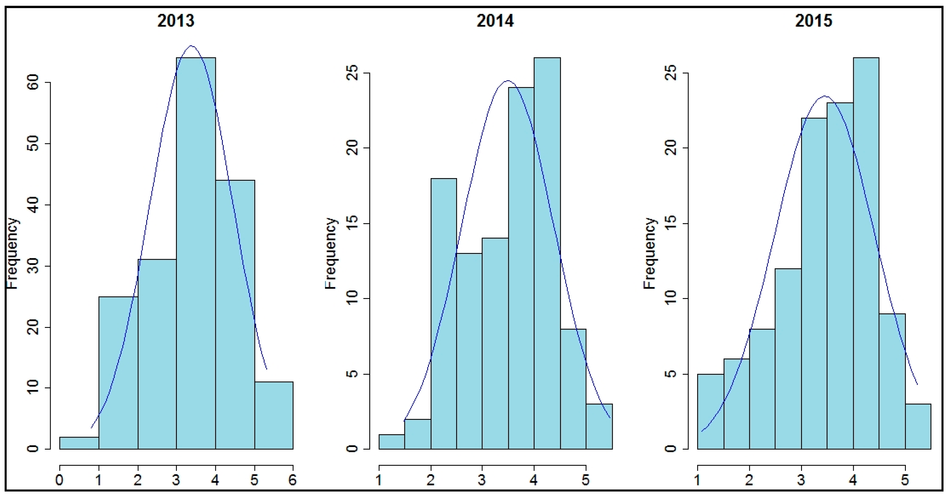
Regardless of the data distribution, kriging can provide the best unbiased predictor of values at unsampled points [35]. Geostatistical methods, however, are optimal when data have close to a normal distribution (lack of strong skewness) to provide the best estimates (e.g., probability maps, confidence intervals). Therefore, it is best to ensure that the data do not significantly deviate from normality. For this reason, the dataset of soil Fe were log transformed (natural logarithm), resulting in more symmetrical distributions that were closer to normal (Figure 4).

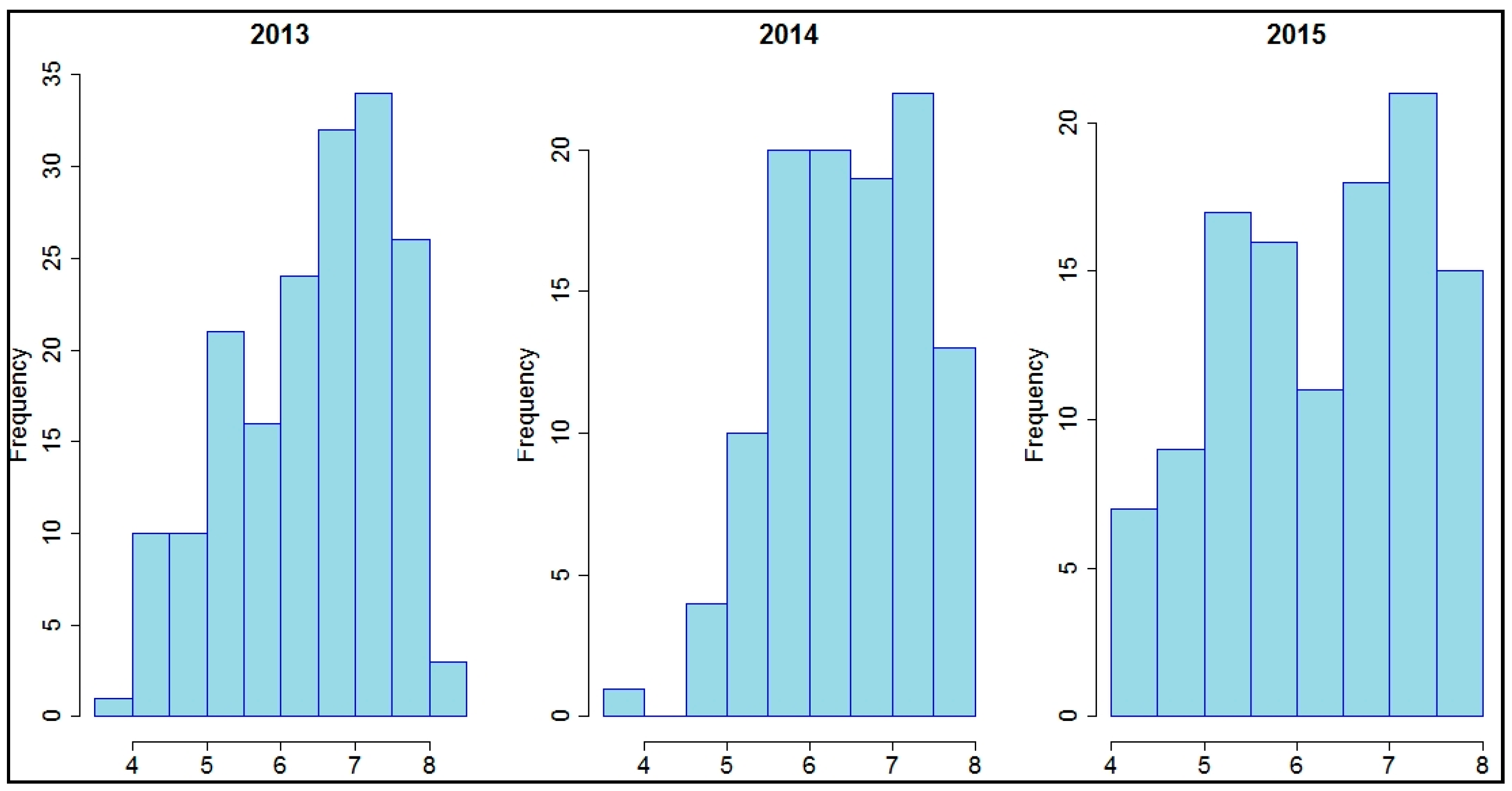
The frequency distributions of pH per year were more symmetrical than those of soil Fe, as seen in the following histogram (Figure 5).

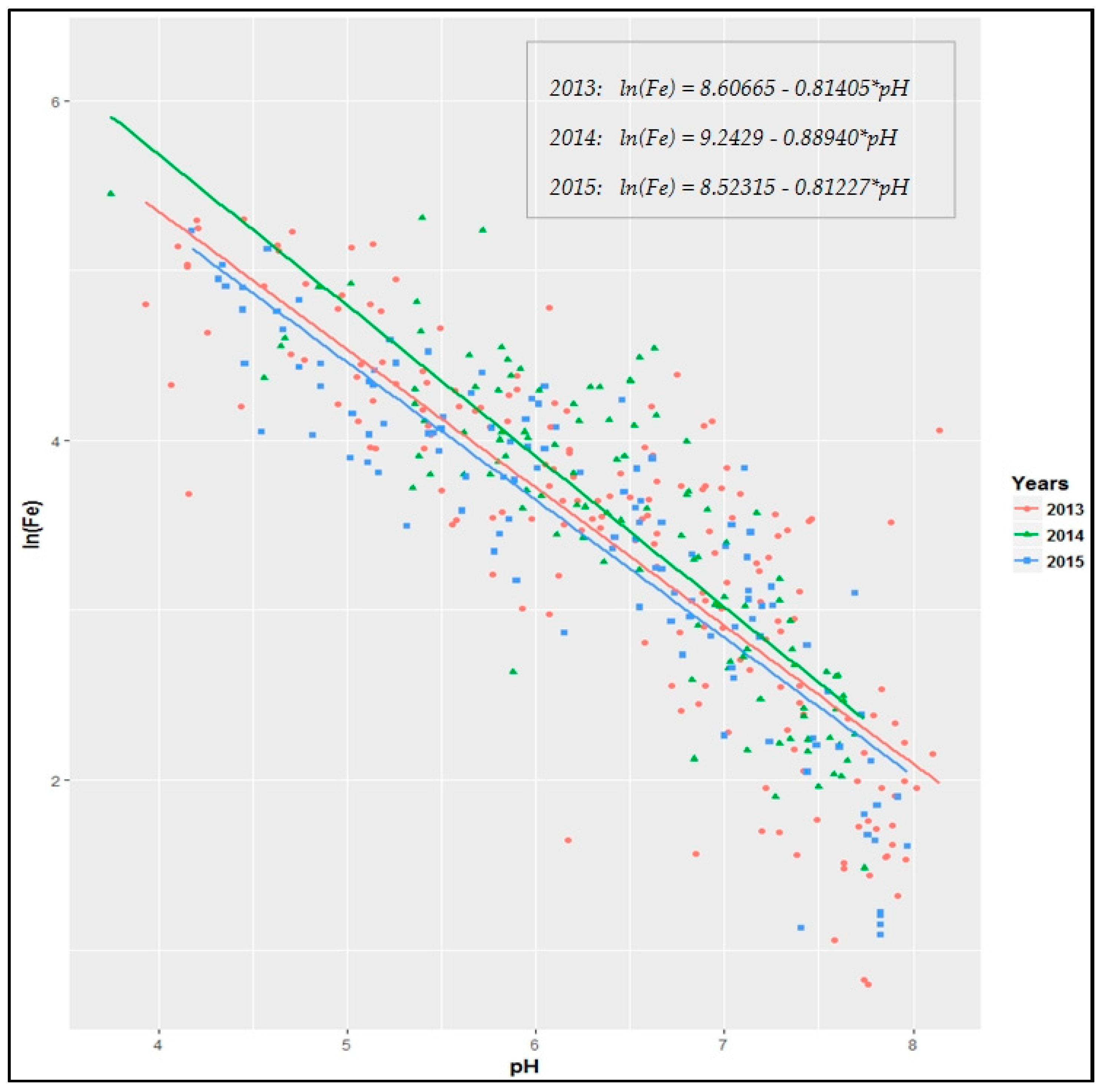
Assessing the correlation between the soil iron (ln(Fe)) and pH by using linear regression analysis of the data in the study area showed a negative correlation between them, which was supported by previous research [22]. There was a statistically significant, moderately strong relationship (at the 95% confidence level) between the two soil variables for each of the years. The correlation coefficient (Pearson’s r) ranged from −0.827 to −0.887 (

Table 2. Correlation parameters between ln(Fe) and pH for each year.

	2013	2014	2015
Pearson’s r	−0.827	−0.842	−0.887

).

Table 2 showed that the fitted linear regression models explained 68%, 70%, and 78% of the variability of ln(Fe) for 2013, 2014, and 2015, respectively, and exhibited quite similar behaviour, having similar regression lines and functions each year, as presented in Figure 6.

It should be noted that the intention for regression analysis presented here was mainly to assess the correlation between the two soil parameters and not to estimate the regression functions between them.

3.2. Semivariograms Analysis

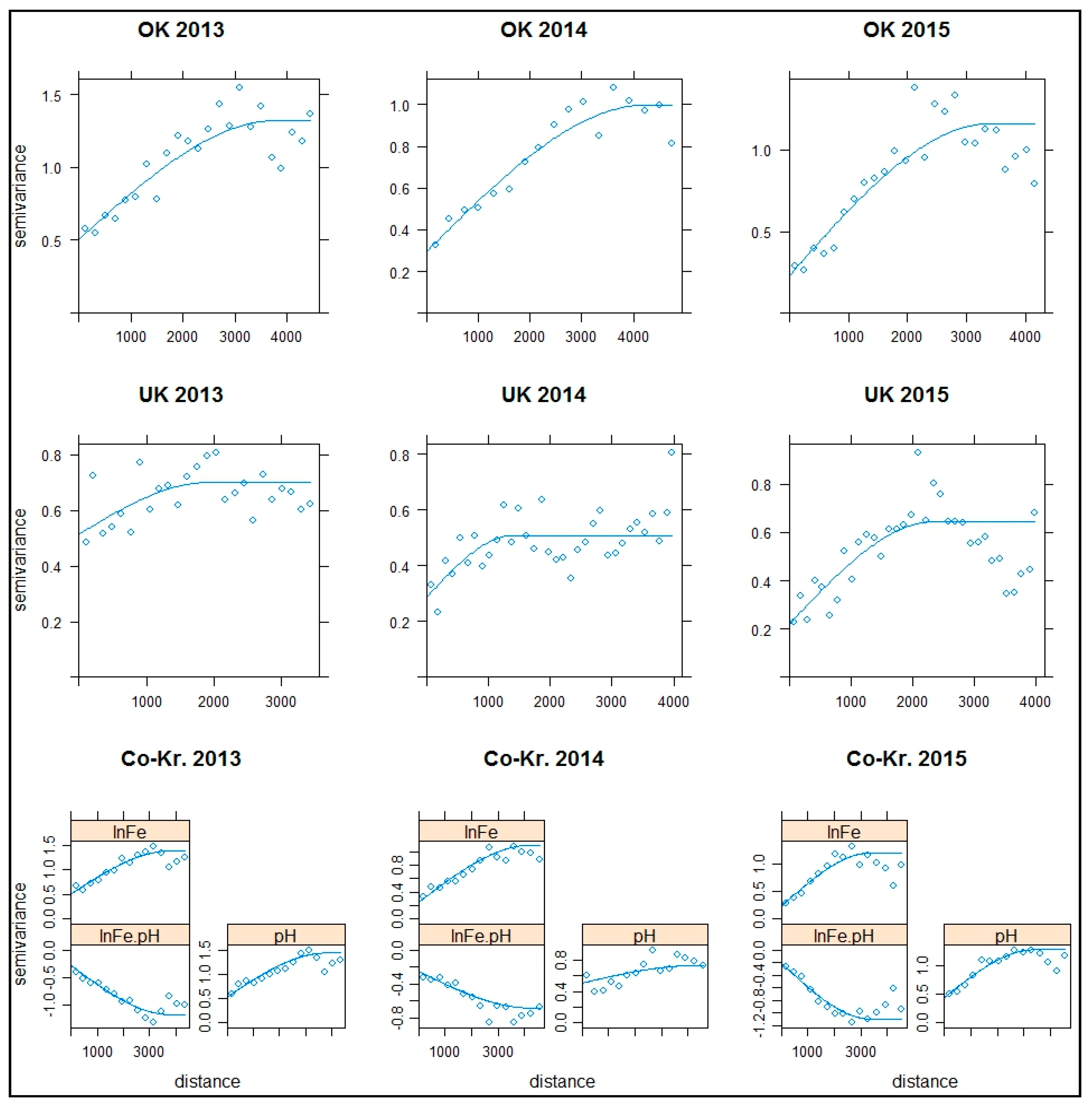
To better assess and compare the interpolation techniques, the models were estimated once and used in the same way in each cross validation. The experimental semivariogram parameters and models were estimated from the randomly selected training set (70% of data) from each year and are presented in

Table 3. The semivariogram models and parameters for the three interpolation methods for each year along with the cross-semivariogram parameters for Co-Kriging. The C₀/C₀ + C₁ is the nugget to total sill ratio. Models were estimated from the training set.

	2013					2014					2015
	Model	Nugget (C0)	Par. Sill (C1)	Range (a) in Metres	C0/C0 + C1	Model	Nugget (C0)	Par. Sill (C1)	Range (a) in Metres	C0/C0 + C1	Model	Nugget (C0)	Par. Sill (C1)	Range (a) in Metres	C0/C0 + C1
OK ln(Fe)	Sph.	0.51	0.82	3795	38%	Sph.	0.30	0.70	4251	30%	Sph.	0.23	0.94	3397	19%
UK ln(Fe)	Sph.	0.52	0.19	1892	73%	Sph.	0.29	0.22	1401	56%	Sph.	0.22	0.43	2351	33%
OK pH	Sph.	0.58	0.74	3458	43%	Sph.	0.36	0.46	4303	43%	Sph.	0.41	0.85	3148	32%
CO-Kr	Sph.	−0.28	−0.89	3795	23%	Sph.	−0.25	−0.43	4251	36%	Sph.	−0.2	−0.89	3396	18%

and Figure 7. In all cases, the optimized semivariogram spherical model (Equation (2)) that best fit the experimental semivariogram was selected.

The negative values of the cross-semivariogram (in Co-Kriging) between soil iron and pH were expected due to a negative correlation between these two variables, as shown in the exploratory data analysis.

For each year, the semivariogram parameters were rather similar for the same interpolation methods.

In OK for ln(Fe), the range was high (from 3397 to 4251 m), with a close partial sill (0.7–0.94). Also, the nugget to total sill ratio was rather low, indicating a moderate to strong spatial dependence, with values from 19% to 38%.

The UK for ln(Fe) had a smaller range (from 1401 to 2351 m) and reduced variability compared to OK, as seen from the lower partial sill values. The spatial dependence was moderate, ranging from 33% to 73%.

The OK for pH had high ranges similar to the OK for ln(Fe), ranging from 3148 to 4300 m. The other semivariogram parameters were also mostly similar. For 2013, all the parameters were very close (C₀ OK: Fe = 0.51, pH = 0.58, C₁ OK: Fe = 0.82, pH = 0.74, range OK: Fe = 3795 m, pH = 3458 m); for 2014, there was a difference in sill (C₀ OK: Fe = 0.30, pH = 0.36, C₁ OK: Fe = 0.70, pH = 0.46, range OK: Fe = 4251 m, pH = 4303 m); and, for 2015, there was a nugget deviation (C₀ OK: Fe = 0.23, pH = 0.41, C₁ OK: Fe = 0.94, pH = 0.85, range OK: Fe = 3397 m, pH = 3148 m). However, the overall similar semivariogram parameters supported that these co-variables exhibited a spatial relationship (in addition to the strong value correlation presented in the regression analysis) that might increase the prediction accuracy in Co-Kriging. The spatial dependence of pH for OK was rather moderate, from 32% to 43%.

Based on the close values in the ranges between OK ln(Fe) and pH for each year, the same range of OK ln(Fe) values was also used for Co-Kriging (each year) as a stable parameter from the semivariogram to the cross-semivariogram (3795 m for 2013, 4251 m for 2014, 3396 m for 2015). The spatial dependence could be characterized as strong to moderate (from 18% to 33%).

Interestingly, the nuggets in each interpolation method for 2013 were similar and much higher than in the other years, which could be random or related to the location/dispersion of the sampling points of this year.

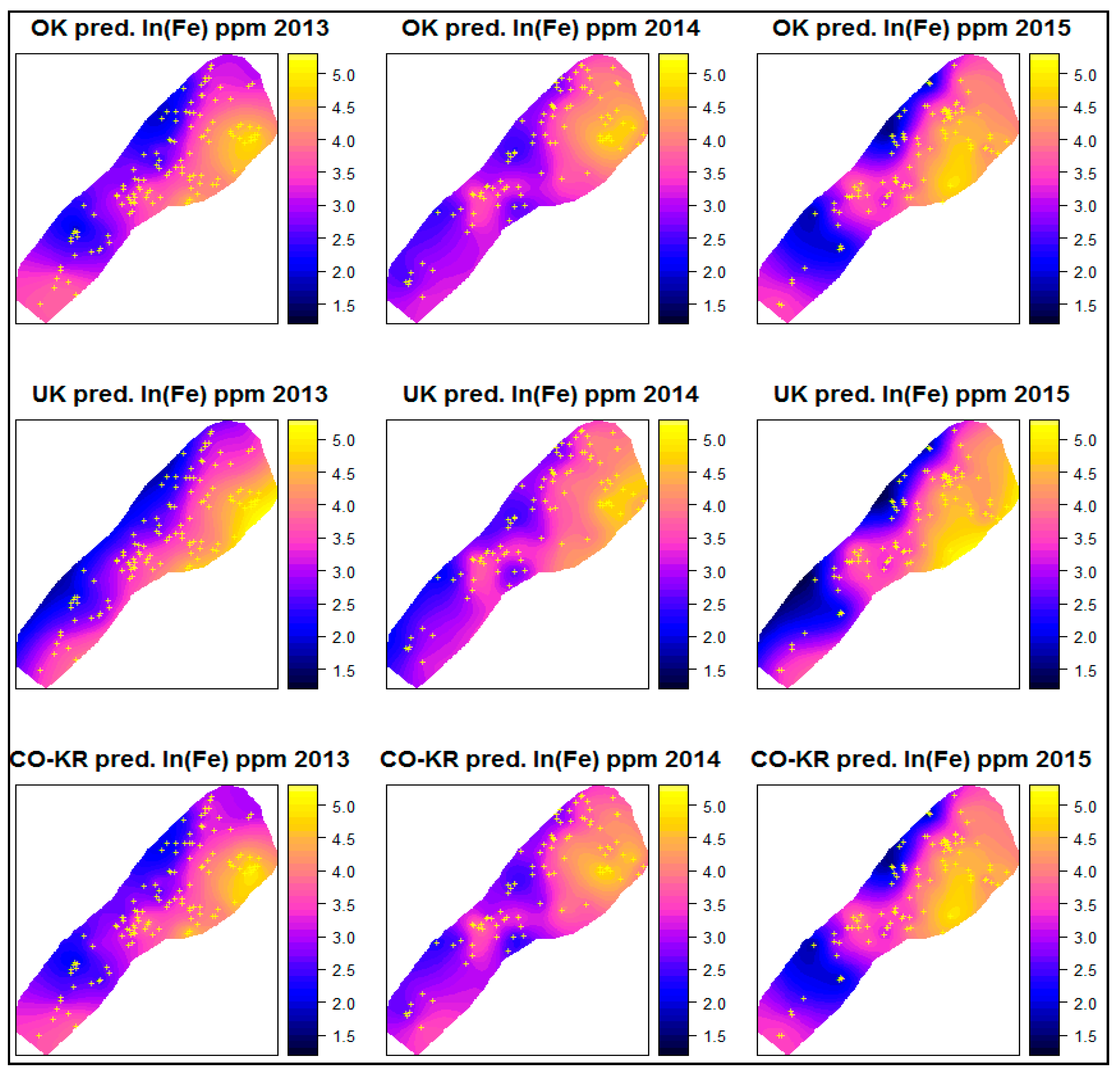
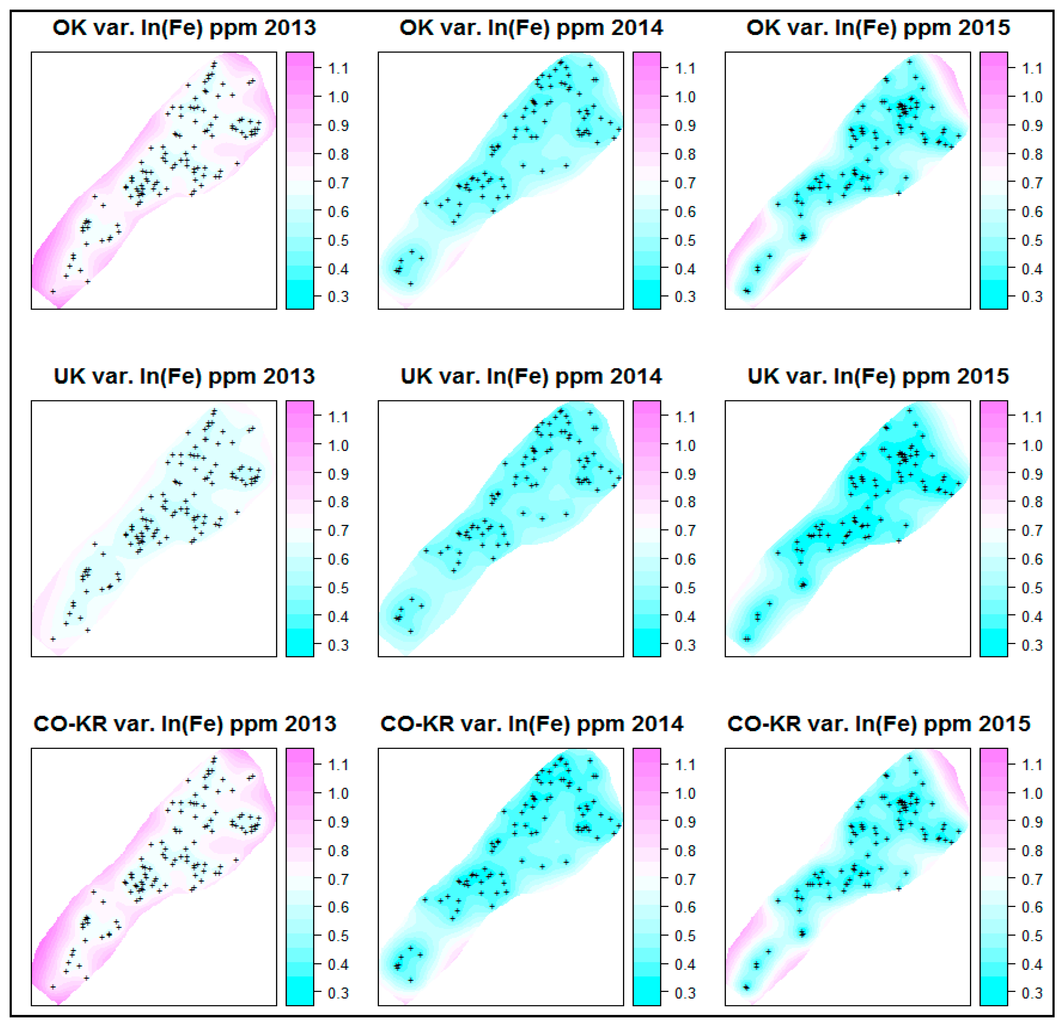
3.3. Prediction Maps and Prediction Error Maps

The prediction maps for each interpolation method and for every year, along with the variances of the prediction maps (prediction errors), are presented in Figure 8 and Figure 9.

For each year, the prediction maps of the different interpolation methods exhibited similar structures with minor differences. Overall, a smooth spatial process was depicted. The areas with high soil Fe concentrations were located at the right side of the maps (yellow colour), further from the lake and at higher altitudes, whereas the areas with lower values were located at the left side of the maps, closer to the lake, and at lower altitudes. Additionally, at the edges of the study area and in some areas in between where there were no sampling points, there were values that were either too high or too low with high prediction errors (mainly interpolation issues due to a lack of data at that point). This can be better assessed by the prediction error maps presented below.

As presented in Figure 9, the 2013 prediction error maps generally had extended areas with high errors (pink colour), possibly due to more concentrated sampling locations (not evenly distributed). The year 2014 had the smallest area, with a high error limited only to the edges of the maps. The next year (2015), the areas with high errors were also limited to the edges of the study areas.

Comparing Co-Kriging with the other interpolation techniques based on only the prediction and prediction error maps provided results that were similar to the OK results without really exhibiting any improvement. On the other hand, the UK interpolation method presented the widest areas with low prediction errors overall (areas with blue colour).

3.4. Cross Validation

Initially, the ‘holdout cross-validation’ method results are presented. In this case, the models that were already estimated from the training set (Table 3) were used for predictions in the test set. As shown in

Table 4. Cross-validation holdout method results of soil Fe predictions. The root mean square error (RMSE), mean error (ME), and mean squared deviation ratio (MSDR) are referring to ln(Fe), for which Fe is in ppm.

	2013			2014			2015
	RMSE	ME	MSDR	RMSE	ME	MSDR	RMSE	ME	MSDR
OK	0.777	0.162	0.885	0.680	0.363	1.108	0.618	0.069	1.003
UK	0.801	0.158	1.028	0.678	0.336	1.135	0.649	0.053	1.210
Co-Kriging	0.772	0.170	0.871	0.638	0.319	1.097	0.618	0.068	0.995

, the prediction errors (RMSE) of soil iron using Co-Kriging were slightly lower than those of the other interpolation methods for every year, except for those of OK for 2015, which were equal (Figure 10). Also, the year 2015 had the lowest prediction errors overall.

The mean error was similar to every interpolating method for each year, having an overall positive bias. Comparing each year, 2014 had the highest ME (>0.3), followed by 2013 (0.1–0.2), and lastly, 2015, with a smaller ME (ME < 0.07).

The MSDR, which ideally should have a value close to one, showed some variation, especially in 2013. The two lower values (0.885 and 0.871) indicated that kriging variances overestimated the squared errors for OK and Co-Kriging. On the other hand, the UK for 2015 had a higher MSDR (1.210), which showed an underestimation of the squared errors.

However, it is important to keep in mind that the holdout method depends heavily on which data points were selected, even at random. Therefore, the ‘leave-one-out cross-validation’ method for soil iron predictions is also presented (

Table 5. The cross-validation results with the leave-one-out method of soil Fe predictions. The root mean square error (RMSE), mean error (ME), and mean squared deviation ratio (MSDR) are referring to ln(Fe), where Fe is in ppm.

	2013			2014			2015
	RMSE	ME	MSDR	RMSE	ME	MSDR	RMSE	ME	MSDR
OK	0.800	−0.0006	1.009	0.632	−0.006	0.945	0.611	−0.005	0.973
UK	0.798	0.0001	1.046	0.625	−0.007	0.954	0.601	−0.006	1.062
Co-Kriging	0.601	0.001	0.880	0.437	0.0004	0.970	0.393	−0.001	0.937

) using the same model as in the holdout method.

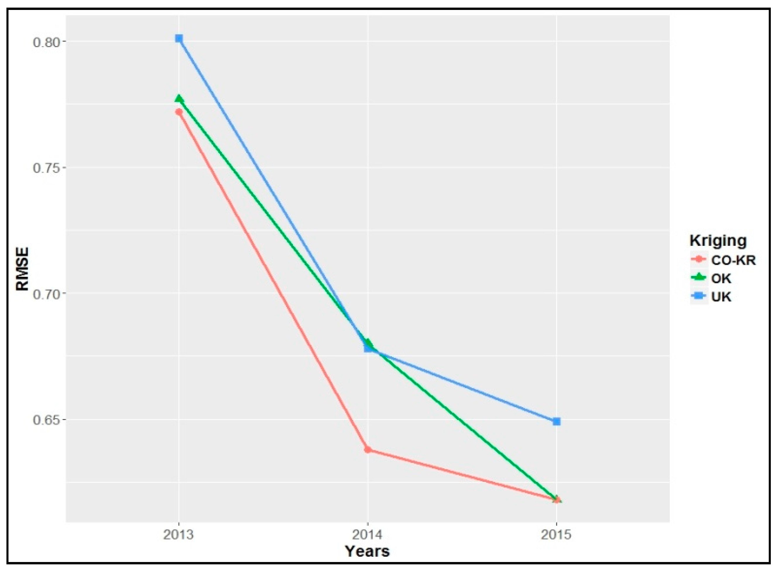
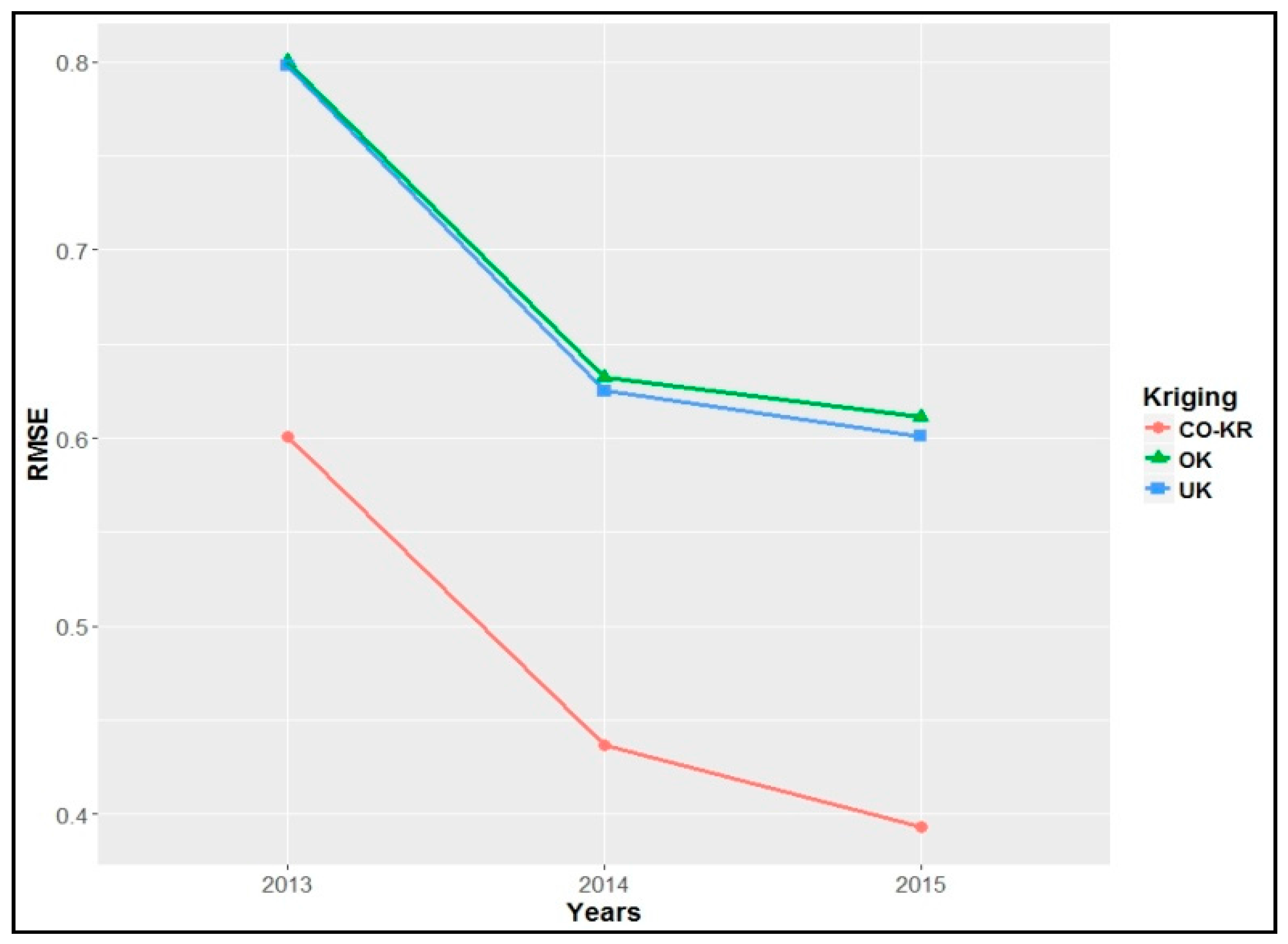
This method had overall similar results with the holdout method regarding prediction errors (RMSE); however, it presented a clear improvement against the Co-Kriging interpolation method in comparison with the other interpolation methods, with an approximately 25%, 30%, and 35% decrease for each year (Figure 11).

Especially for 2014 and 2015, there were significantly lower prediction errors than in the holdout method. Additionally, in the LOOCV method, the mean errors were lower (smaller bias) than in the holdout method, something that was rather expected [27,36]. Finally, the MSDR was more evenly distributed and overall closer to one.

4. Summary and Conclusions

In the current study, three different interpolation methods, including Ordinary Kriging, Universal Kriging, and Co-Kriging, were performed and compared to predict the spatial distribution of soil iron. For this reason, 400 soil samples from the Kozani area, near Polifitou Lake in northern Greece, were randomly collected from 2013 to 2015 and analysed in the laboratory to determine the soil Fe concentrations and pH. A subset of these data was randomly selected (70%, the training set) to estimate the models, and the remaining data (30%, the test set) were used to validate the results.

Initially, assessing value correlations between the soil iron (ln(Fe)) and pH, with the use of a linear regression analysis of all the data in the study area, showed a statistically significant, moderately strong, negative correlation between the two variables. The linear regression models explained 68%, 70%, and 78% of the variability of iron in 2013, 2014, and 2015, respectively, and showed quite similar behaviour, with similar regression equations for each year.

Estimating and studying the semivariograms for the different interpolation techniques for each year showed that the OK for pH had high ranges similar to the OK for ln(Fe). The other semivariogram parameters were also rather similar, supporting the idea that these co-variables exhibit a spatial relationship that could be used for Co-Kriging and that could possibly increase the prediction accuracy.

Based on the prediction maps and prediction error maps throughout, this result was not obvious. Instead, the UK presented better results, including the largest areas with low overall prediction errors.

However, comparing Co-Kriging with the other interpolation techniques using cross-validation showed an improvement in the prediction accuracy, with smaller prediction errors (RMSE) overall. In the holdout method, the improvement was less prevalent, but improvement was substantial in the leave-one-out cross-validation method based on prediction errors that were significantly lower than the other two interpolation methods.

Notably, the difference between the two cross-validation methods was expected based on their methodological differences. However, this difference does not imply that one method (e.g., the one with lower RMSE) is better than the other. Each method has its advantages, disadvantages, and uses. What is important is that both methods exhibited an increased Co-Kriging prediction accuracy compared to the other interpolation techniques in the current study.

These findings are in accordance with previous research indicating that a strong correlation between variables leads to improved results in Co-Kriging [14,37,38]. Having the secondary parameter (pH) more extensively sampled could potentially further improve its prediction accuracy [3,39].

For future work, different areas could be sampled and studied with different sampling densities between the primary and auxiliary parameter. Other cross-validation methods might also be used (e.g., k-fold, Monte Carlo), and potential differences could be assessed.

Finally, this study shows that the use of multivariable geostatistics (here Co-Kriging) by taking advantage of possible variables and data in an area can be effective if there are spatial relationships among these variables that can be appropriately modelled.