An Adaptive Sweep-Circle Spatial Clustering Algorithm Based on Gestalt


1
School of Urban Design, Wuhan University, 129 Luoyu Road, Wuhan 430079, China
2
Collaborative Innovation Center of Geospatial Technology, 129 Luoyu Road, Wuhan 430079, China
3
Department of Civil and Surveying Engineering, Guilin University of Technology at Nanning, 15 Anji Road, Nanning 532100, China
4
Land and Resources Information Center of Guangxi Province, 2 Zhongxin Road, Nanning 530028, China
*
Author to whom correspondence should be addressed.
ISPRS Int. J. Geo-Inf. 2017, 6(9), 272; https://doi.org/10.3390/ijgi6090272
Submission received: 20 July 2017
/
Revised: 17 August 2017
/
Accepted: 24 August 2017
/
Published: 30 August 2017
Abstract
:An adaptive spatial clustering (ASC) algorithm is proposed in this present study, which employs sweep-circle techniques and a dynamic threshold setting based on the Gestalt theory to detect spatial clusters. The proposed algorithm can automatically discover clusters in one pass, rather than through the modification of the initial model (for example, a minimal spanning tree, Delaunay triangulation, or Voronoi diagram). It can quickly identify arbitrarily-shaped clusters while adapting efficiently to non-homogeneous density characteristics of spatial data, without the need for prior knowledge or parameters. The proposed algorithm is also ideal for use in data streaming technology with dynamic characteristics flowing in the form of spatial clustering in large data sets.
1. Introduction
Rapid advancements in geographic spatial information technology, generation, and collection have created exponential growth in spatial data, which has resulted in increasingly complex data structures. It is increasingly necessary to address the challenges involved in extracting useful information and knowledge from large-scale and highly complex spatial data sets. Data mining from the spatial data set is a valuable way to obtain valuable information, with spatial clustering having played an indispensable role in spatial data mining research. Clustering is the process of grouping spatial data objects into a series of meaningful clusters so that objects within a particular cluster share similarities, while being dissimilar to other clusters [1,2]. Spatial point clustering has been applied to a wide variety of fields, including urban planning, remote sensing, geographic information, bio-engineering, geology and minerals, as well as computer science [3,4,5]. The current methods for spatial clustering have been roughly classified into the following categories:
These traditional approaches have been successful in managing a number of specific applications across different domains, but significant limitations exist. Most traditional clustering methods rely on user-specified arguments or a priori knowledge. Furthermore, these methods cannot manage clusters of irregular shapes or of different sizes and are not effective in sets with non-uniform inner density, outliers, or noise. In fact, no particular clustering method has been shown to be superior to its competitors with regards to all of the necessary aspects [25,26]. To date, the advantages and disadvantages of various algorithms have been extensively analyzed [26,27,28,29,30,31]. An analysis of the classical spatial clustering algorithms is shown in Table 1.
Data often involve the relation to geographical space and are processed in large amounts. The spatial object is highly complex and requires extensive computation, which means that clustering algorithms need to be highly efficient. Efficient spatial clustering algorithms are valuable for many real-world, dynamic applications [32]. Large data sets are challenging for computational systems when processed with conventional algorithms, particularly as the amount of spatial data increases exponentially in the real world. Popular traditional clustering algorithms require repeated access to the data set as well as multiple clustering operations, which means that their efficiency decreases with an increase in data set size [5,27,33]. This paper proposes an adaptive spatial clustering algorithm (ASC) that employs both sweep-circle techniques and a dynamic threshold setting based on Gestalt theory to detect spatial clusters. Empirical results and a comparison with traditional methods demonstrated that the proposed ASC can automatically discover clusters in one pass, rather than modifying the initial model. A minimal spanning tree, Delaunay triangulation (DT), or Voronoi diagram can be quickly identified even with arbitrarily-shaped clusters. The proposed ASC can identify the non-homogeneous density characteristics of spatial data without the need for prior knowledge or parameters. It is compatible with streaming dynamic, large-scale data found in spatial clustering.
The remainder of this paper is organized as follows: In Section 2, the relation of ASC to previous methods is described. In Section 3, the proposed algorithm is explained in detail. Section 4 describes the ASC-based streaming process as applied to large data sets. Section 5 reports our analysis of the algorithm, including its time complexity and comparison with other clustering methods. Section 6 provides an example of the proposed algorithm applied to a real-world data set, while Section 7 concludes with an outlook for further research.
2. Related work
2.1. Plane-Sweep Techniques
The plane-sweep is a popular acceleration technique used to solve 2D Euclidean space geometric problems [34]. This technique initially sorts the geometric elements, before imagining that a sweep-line glides over the plane and stops at geometric elements (typically called “event points”) [35], where the corresponding data structure is then updated. The plane-sweep method cannot move backwards across the event points.
The sweep-plane technique was initially applied to computational geometry problems [36]. Shamos and Hoey later applied a unidirectional sweep-plane algorithm that used time O (nlogn) to determine whether or not a finite number of line segments have any intersections in a plane [37].
Bentley and Ottmann extended this algorithm to determine the existence of intersecting line segments. Furthermore, they were able report all k intersections of n line segments within time O ((n+k)logn), where k is the number of intersections [38]. The sweep-line algorithm was also used to construct a Voronoi diagram, i.e., dual Delaunay triangulation [39]. The Delaunay algorithm examined in this study is based on the plane-scattered point sets used by Žalik [35] and Zhou [40]. Žalik was the first to suggest the use of sweep-line techniques for spatial clustering [41].
2.2. Sweep-Circle Algorithm
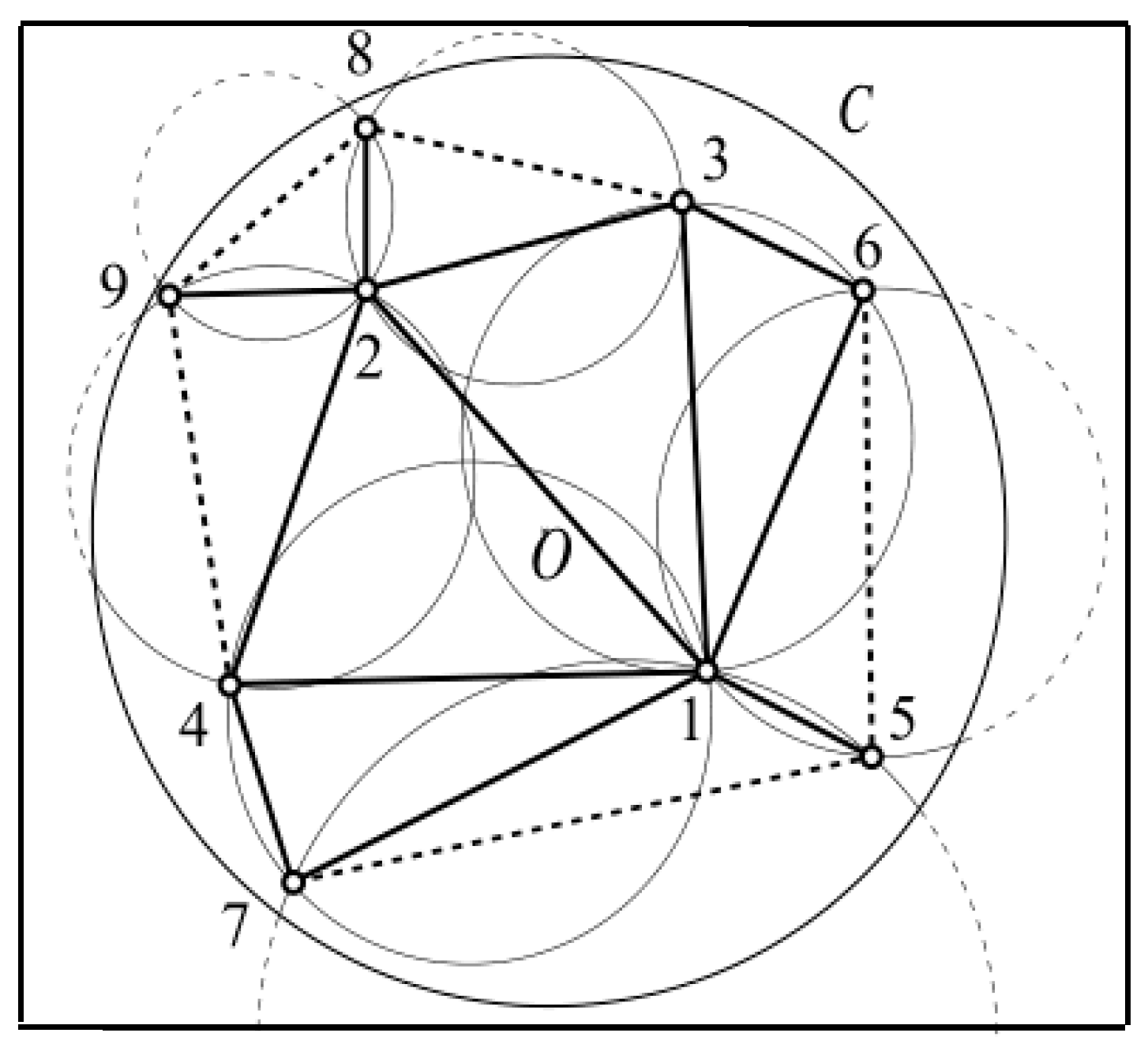
The sweep-circle is another important sweep-line technique, where points are initially sorted according to their distances from a fixed pole O in the convex hull of S. It is assumed there is a circle C centered at O, with radius increasing from 0 to +∞, which stops at event points and updates the data structure. A part of the problem being swept (inside the circle) is already solved, while the remaining part (out of the circle) is unsolved. Dehne and Klein [42] were the first to use a circle that emanates from a fixed point, which resulted in a Voronoi diagram. Adam [43], in addition to Biniaz and Dastghaibyfard (2012), suggested that the incremental sweep-circle algorithm was more suitable for constructing Delaunay triangulations [42] (Figure 1).
2.3. Data Stream Technique
The “data stream” is an unbounded orderly sequence of information, which can consecutively arrive in large quantities. However, this technique can only process data sequentially with appropriate access. Data mining algorithms based on data streaming techniques are commonly used in obtaining data from satellite remote sensors, geographic information, network monitoring, and financial services. Traditional typical spatial clustering algorithms that repeatedly access entire data sets cannot be readily applied for data streaming, as their high complexity and computational cost makes it impossible for them to manage such a large amount of data. In fact, data stream clustering algorithms have become important in data mining research and subsequently, many algorithms based on data stream technology have been proposed, including the commonly-used one-pass algorithm [9,44,45,46,47,48]. This algorithm divides the non-streaming data sets into data blocks so as to fit requirements of the memory space and one-pass sweeping data objects. The traditional clustering algorithm can be applied to the data-streaming environment once the data blocks have arrived from the data stream [49]. For example, K-Means and K-Medians algorithms [44] can be used to process large data sets, before the Squeezer algorithm can allocate the data into similar globes for clustering using one-pass sweeping [46]. The BIRCH algorithm uses a clustering feature tree to minimize I/O requests prior to the one-pass sweeping for clustering [9]. Guha et al. also conducted valuable research on the one-pass algorithm using similar data sets [44,47].
2.4. Sweep-Line Clustering Algorithm
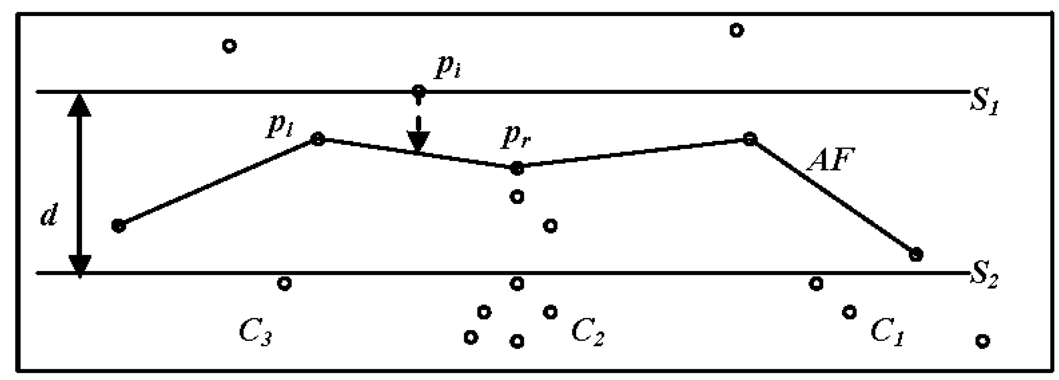
Žalik (2009) proposed an innovative, agglomerative hierarchical clustering algorithm for spatial data using a sweep-line in O (nlogn) time in the worst case. This algorithm does not rely on domain knowledge or modification of the initial model. Furthermore, this algorithm can determine clusters of arbitrary shapes when completing spatial clustering of large data sets. In this algorithm, there are the horizontal sweep-lines named S1 and S2, where the distance from S1 to the front of S2 is d. It is assumed that S1 sweeps the pi-1 set points in accordance with the proximity parameter d to form part of the clusters, while the points of the front line (AF) are sorted in accordance with the x coordinates. When S1 encounters point pi, pi is projected to the frontier toward AF and a cluster is found by comparing the distance from pi to pl and pi to pr using the proximity parameter d (Figure 2). When S1 moves to the next point, S2 follows it at distance d. The points that have been swept by S2 are removed from the AF. If the projection misses the AF (that can also be empty), the corresponding end-point of the AF is tested to determine whether it is close enough to point pi to discover a new cluster [41]. It is difficult to determine the global parameter d that accounts for uneven distribution of data sets. If the parameters are set without a priori knowledge (or measured experimental results), it is difficult to find true clusters accurately.
3. ASC Algorithm
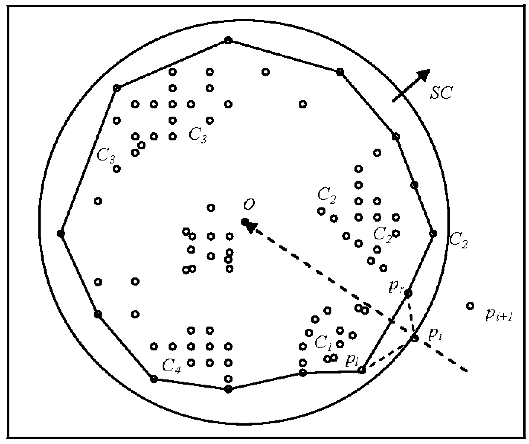
Let E be the Euclidean plane and the Euclidean distance between two points x and y of E; and S be a planar set of n points of E, which are called sites. In the polar coordinate system where the ASC algorithm is applied, pi is swept from the initial frontier in the outwards direction according to the increasing distance from pole O (i.e., the sweep-circle center). Following this, pi is projected onto the segment of frontier edge (plpr) along the circle in the O-direction (Figure 3). According to Tobler, the first law of geography is that “everything is related to everything else, but near things are more related than distant things” [50]. The points are considered to be similar if the points are within a specific distance of each other, such as points pi and pl or pi and pr (Figure 3). These values fall under a threshold value used to determine the formation of clusters.
The algorithm proposed in this paper utilizes the Gestalt theory and the associated definition of the dynamic adaptive threshold. It can efficiently locate the adaptive clusters of arbitrary shapes and can acclimate to the uneven density characteristics of spatial data to avoid the requirements of preset global parameters, such as those necessary for DBSCAN, DENCLUE, and other algorithms [41]. ASC works in a four-phase process: basic conceptualization, initialization, clustering, and cluster merging.
3.1. Basic Concepts and Initialization
Cluster definitions. Given n collection of discrete points S = {p1,p2,p3,···,pn} in 2D set (R2), we use the degree of similarity between data points. Thus, the data set divides S into k clusters C = {C1,C2,…,Ck} C S for defining the cluster, where = S, (i≠j). This will result in the clustering of objects with high similarity, and the division of objects with high dissimilarity into different clusters.
Determining the center of the sweep-circle. S corresponds to the coordinate set {p1 (x1,y1), p2 (x2,y2), p3 (x3,y3),···, pn (xn,yn)}, where the origin of the polar coordinate O (px,py) is the center of the sweep-circle. Select O (px,py) as the average of the largest (xmax,ymax) and smallest (xmix,ymix) values of input S.
Calculating the polar coordinates of input points and sorting. The polar coordinates of input points are calculated and sorted by increasing distance from O as follows:
Each point pi (xi,yi) in the Cartesian coordinates can be transformed to pi (ri,θi), where the points are sorted according to their r-coordinate found in the polar coordinates. If two points have the same r-coordinate, they are sorted by the secondary criterion θ. In a special case where the first point coincides with the origin O (i.e., its r-coordinate is zero), the point is removed from the list.
Constructing the initial frontier and clusters. The three points located nearest to the center O are used to form a triangle, where it is assumed that the three points are non-linear. The three edges of the triangle form a polyline, which is referred to as the frontier. Any spatial clustering algorithm should work based on various distances, such as the Euclidean distance, the Manhattan distance, or the Minkowski distance. This algorithm uses the Euclidian distance between data points to measure the distance needed for spatial clustering. Figure 4 shows an example of the three points nearest to the center O, which forms the initial cluster.
Clustering the threshold. The threshold setting is set as the distance measurement of d (pi,pj), which determines if two points are grouped into the same cluster. If the distance between the two points is less than or equal to this value, they belong to the same cluster; otherwise, they do not. This is calculated as follows:
Cp = ∪ {pi,pj} |d (pi,pj) ≤ ε, (j ≠ i, pi, pj∈S)
The clustering process for the global threshold setting is sensitive to density changes, particularly the internal density changes within the clusters. To manage the gradual changes of the local density, we used the fact that the spatial data mining process obeys not only the objective law of the geographical entity itself, but also relates to the concept of recognition in cognitive psychology. Specifically, the Gestalt theory was taken into account.
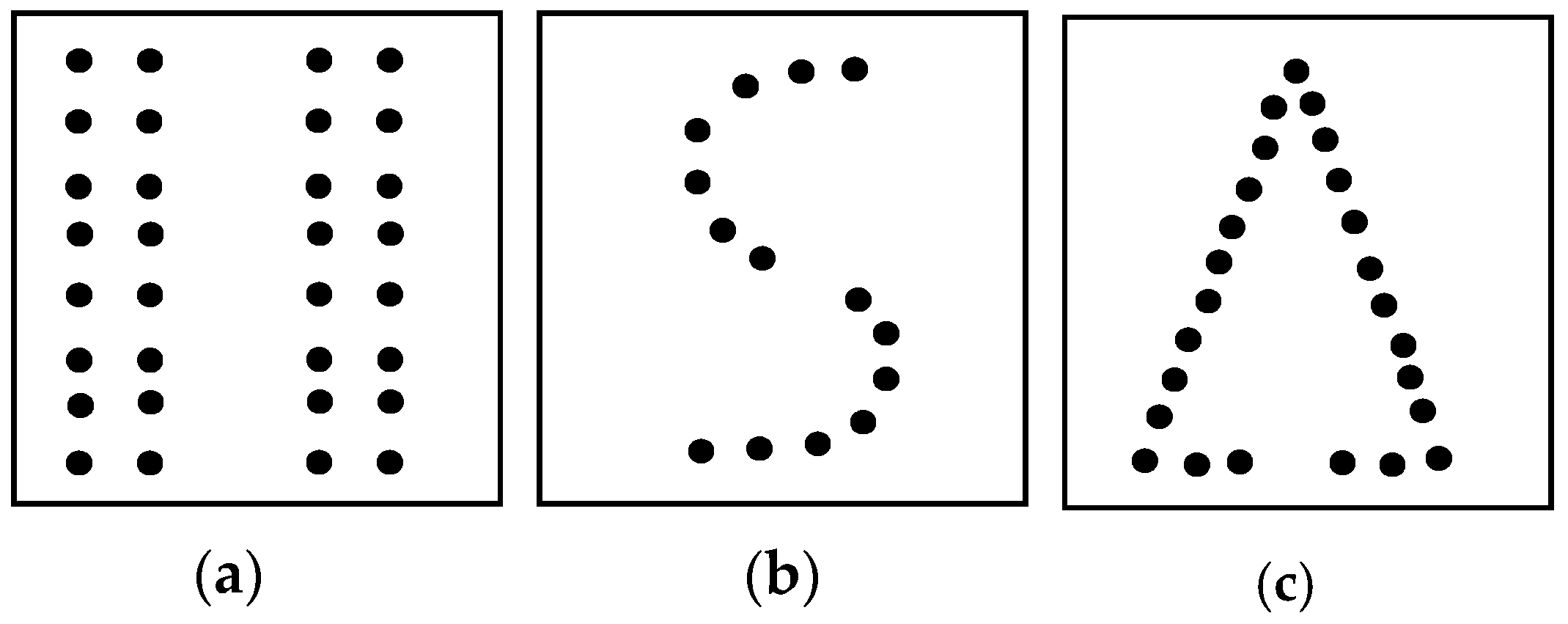
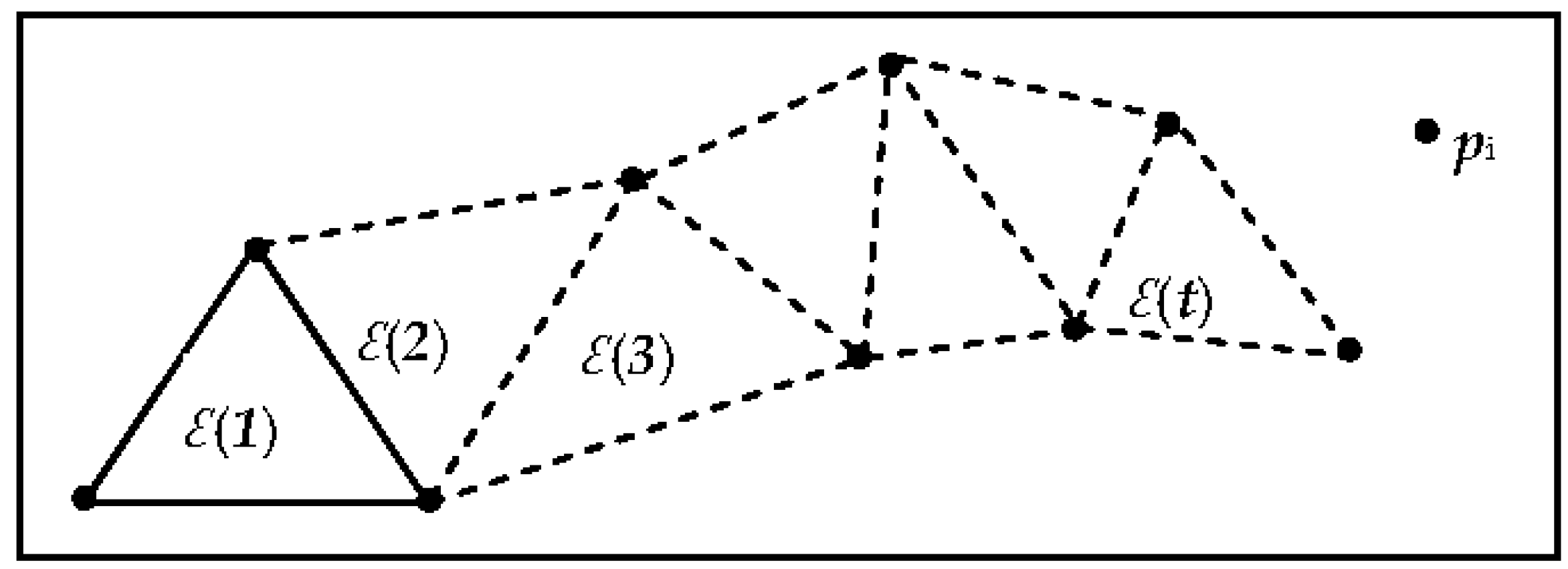
The Gestalt theory summarizes the cognitive law of human vision with the pattern organization discipline generated by the Gestalt principle, having been applied in pattern recognition and spatial clustering [14]. The main principle of the Gestalt perception model is that “the whole is greater than the sum of its parts,” which suggests that people tend to perceptually recognize structural integrity and can initially observe the visual object as a whole before breaking the object down into different parts [14]. Gestalt is interpreted through principles of visual recognition, such as proximity, similarity, closure, continuity, orientation, and common fate [51].We combined a subset of Gestalt principles operating simultaneously to build the dynamic adaptive threshold model (t). We can define the mean of the triangle’s perimeter Lt as the adaptive dynamic threshold (t). In this model, each new event point pi is processed to correspond to the threshold according to the following three Gestalt principles (Figure 5).
• Proximity, where objects placed close together tend to be perceived as a group.
In agreement with Tobler’s First Law of Geography, proximity is the most important for spatial clustering (in addition to also being the basis of continuity and closure). The easier it is to form continuity and closure among spatial data, the greater the similarity.
To build the dynamic threshold, relationships in terms of proximity help to define concepts, such as “distance” and “place”. The concept of ‘distance’ explains the tendency to form a cluster when pi is close to two points of △ (t), while the concept of ‘place’ means that two triangles are adjacent to each other, such as △ (1) and △ (2), or △ (2) and △ (3). These can be used to form the dynamic threshold (1), (2), (3), ··, (t) as a group (Figure 6).
• Continuity, where spatial objects arranged in a logical order are easily perceived as a group or a continuous graph.
The dynamic thresholds require a particular order and continuity relationships create formats, such as a “series”, which are perceived in a more permanent way as the principle of continuity is connected with the concept of integrity in perception.
• Closure, where the observer tends to prioritize closeness and “perfection” of objects. Thus, gaps between objects may be perceived as being filled to create a unified whole.
Closure tendency is valid for visual stimuli. Figure 6 shows that pi has a tendency to connect ∆ (t), which serves as a reminder of the whole.
Accordingly, when the event point pi is projected onto the frontier toward O, the triangle including the frontier is identified and we can define adaptive dynamic threshold (t) as follows:
where is a constant factor. We can enlarge or reduce (t) by manipulating the value of , although this may affect the quality of clusters and reflect the hierarchical relation. The value of is usually set to 1 for ASC.
The three Gestalt principles operate simultaneously within ASC to build the dynamic adaptive threshold model (t), which is shown in Figure 7. The input point p4 is an event point projected on the edge (p2,p3) of triangle ∆p1p2p3 toward O, where p4 is closest to p2 and p3. This results in the formation of a cluster due to the rule of proximity. Under the closure rule, p2 and p3 combine with p4 to form a simple triangle ∆p4p2p3 adjacent to ∆p1p2p3 with a common edge (p2p3). Both the proximity and continuity Gestalt clusters occur at triangle ∆p4p2p3 and ∆p1p2p3, which maintain closely related spatial properties. Therefore, the distance of p4 from p2 and p3 is used to form a cluster, where the mean of the perimeter (L1) of triangle ∆p1p2p3 forms the adaptive dynamic threshold (1). When a new event point p5 is obtained, the mean of the perimeter (L2) of triangle ∆p2p4p5 serves as the adaptive dynamic threshold (2).
Thresholds similar to these are often set in similar real-world applications for use in situation-specific guidelines for users. For example, during urban planning, the threshold value is set according to the minimum radius of the public service area being covered. The threshold can vary, which still allows for the analysis of the distribution of buildings in residential, commercial or industrial areas. Furthermore, this threshold reflects the hierarchical structure of the relationships between different structures.
3.2. Clustering
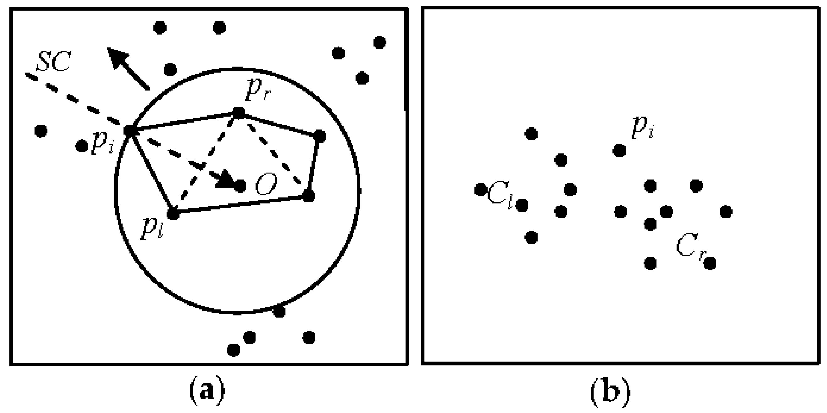
In a system where the sweep-circle SC has already passed the first three points and has assigned them to one cluster, an algorithm surrounds the points by single-closure bordering polylines (i.e., the frontier) as shown in Figure 8a. When SC increases and sweeps to the new point pi, the projection of pi hits the edge (pl,pr) of the frontier toward O. This manner of projection will typically hit the frontier, since the O lies inside the frontier and the new points lie outside of it. By connecting pi and pl as well as pi and pr, the distances dist (pi,pl) and dist (pi,pr) are calculated, where the threshold (t) can be set accordingly. According to Equation (3), there are four possibilities when moving forward:
- dist (pi,pl) > (t) and dist (pi,pr) > (t), where pi is the first element of a new cluster.
- dist (pi,pl) > (t) and dist (pi,pr) ≤ (t), where the right side of pi is assigned to a cluster (Cr) (Figure 8b).
- dist (pi,pl) ≤ (t) and dist (pi,pr) > (t), where the left side of pi is assigned to a cluster (C1) (Figure 8b).
- dist (pi,pl) ≤ (t) and dist (pi,pr) ≤ (t), where if pl and pr are members of the same cluster, before pi is placed into the same cluster. Otherwise, pi is a merging point between left and right clusters [41].
The frontier plays an important role in the process of the discovery of clusters. In order to effectively implement the frontier, heap or balanced binary search trees (e.g., AVL tree, B-tree and Read-Black tree) can be often selected. In our case, a simple hash-table on a circular double-linked list is used to implement the algorithms efficiently and to ensure that large data sets were manipulated correctly (Figure 9). Each record of the frontier stores the key vertex index Pi and the index of the triangle Ti sharing its edge with the frontier (generating an adaptive threshold), in addition to the generated initial clustered index Ci. Fortunately, ASC will not have a projection-missed frontier, as previously mentioned in the literature [41].
3.3. Merging Clusters
The indices of clusters must be merged, i.e., the initial clusters must be adjusted during the final phase in accordance with the merged points. We used a previously applied method [41] to merge the indices of the clusters (Figure 8b provides an example). In this example, the clusters Cl and Cr are merged via pi and the smallest index value is preserved. In each list, any point that does not belong to any cluster is treated as an outlier/noise.
3.4. Point Collinearity
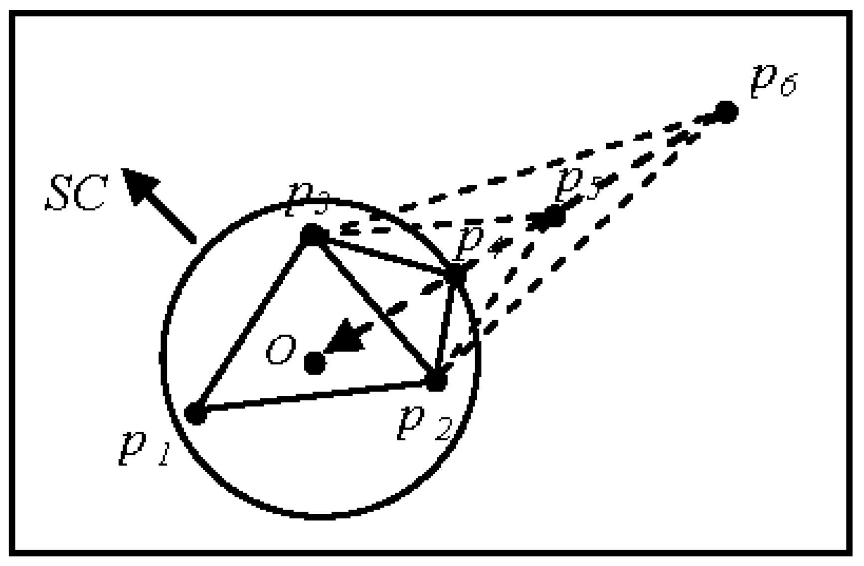
In the ASC algorithm, the “point collinearity” occurs when more than one spatial point is located on the same θ of the polar coordinates. This is a special case that must be treated accordingly in terms of setting the adaptive threshold (t) to ensure the stability of the algorithm. The mean of the triangle perimeter (including previously even points) is defined as the adaptive dynamic threshold that occurs when the sweep-circle located a new even point. When the projection of the next point p5 hits the vertex p4 of the triangle ∆p2p4p3, the mean of the perimeter can be calculated as the threshold, which determines whether the points p4 and p5 are grouped into the same cluster (Figure 10).The threshold of p6 is obtained according to the triangle ∆p2p5p3.
We have described the procedure through a pseudo-code form in Algorithm 1.
| Algorithm 1. ASC clustering algorithm. |
| Input: The 2D set S = {p1,p2,p3,···,pn} of n points |
| Output: C |
| Initialization: |
| 1: select the pole O |
| 2: calculate pi (ri,θi) for points in S |
| 3: sort the S according to r |
| 4: create the first triangle |
| 5: compute (t) ,t←1,t < (n − 3) |
| 6:CL←Ø, CR←Ø,CN←Ø, CS←Ø |
| Clustering: |
| 7: for i ←4 to n do |
| 8: (t) = 1/3 Lt |
| 9: project pi on the frontier; hits the edge (pl, pr) |
| 10: if d (pi,pl) > (t) and d (pi,pr) > (t) then |
| 11: CN←CN∪pi |
| 12: end if |
| 13: if d (pi,pl) > (t) and d (pi,pr) ≤ (t) then |
| 14: CR←CR∪pi |
| 15: end if |
| 16: if d (pi,pl) ≤ (t) and d (pi,pr) > (t) then |
| 17: CL←CL∪pi |
| 18: end if |
| 19: if d (pi,pl) ≤ (t) and d (pi,pr) ≤ (t) then |
| 20: CS←CS∪pi |
| 21: end if |
| 22: create triangle ∆i,l,r |
| 23: t←t + 1 |
| 24: end for |
| Merging: |
| 25: C←CL∪CR∪CN∪CS |
4. ASC-Based Stream Clustering
Bezdek and Hathaway categorize any data set containing 108 objects as a “large data set” [52]. ASC extends the streaming clustering technique to include large spatial data sets repeating a small number of sequential passes over objects (ideally, single passes) and clustering the objects using the average memory space, where the size is a fraction of the stream length. The ASC-based stream clusters use a two-stage online and offline approach, as found in most streaming algorithms. In the online stage, the data set is split into blocks that are divided until they fit into the computer’s main memory bank as the data points are swept within an increasingly large circle. ASC is applied until all spatial data objects in the blocks are processed. In the current experiment, we implemented cluster indexing, which stores the data in units of clusters grouped by ASC within storage systems. In the offline stage, the user sets the threshold and the corresponding clustering number K is identified. Atom clusters in the online stage are repeatedly computed via ASC until the process is complete and the results are provided.
Online stage
- The large data set S is divided into a sequence of data blocks S = {X1,X2,…,Xi} according to the memory size. A load monitor [53] ensures that the loading of spatial data fits the main memory.
- ASC is applied to each data block Xi to form atom clusters Ci = {C1,C2,…,Cl}.
Offline stage
- It is assumed that the user provides a suitable threshold value and the clustering number K is set in advance for the obtained atom clusters. ASC is repeatedly implemented until forming a final (macro) space cluster by processing retrieval queries from the cluster indexes into the adjacent data blocks.
The above algorithm can manage static data and can be extended for the processing of dynamic data.
5. Results and Discussion
5.1. Time Complexity Analysis
All space points n are transformed to polar coordinates in O (n) and sorted according to their r-coordinates by Quicksort in O (nlogn).The total time complexity of the initialization phase is:
Tinti = O (n) + O (nlogn) = O (nlogn)
The sweep-circle status is represented by the frontier, where points must be located to identify those that hit the projected edge. This point location is found in the hash table. A previously reported formula was used [35] to determine the number of entries into the hash-table in ASC:
where h is the size of the hash-table, n is the number of table entries and k is the constant factor.
According to a previous analysis [35], the relationship between CPU time spent and the number of entries into the hash-table h changes according to the value of k. If k is too small or too large, the computational time will be significantly altered. The k was set to 100 for these experiments in accordance to previous literature [35]. During the sweeping phase, each point was projected onto the frontier, where it reached the frontier in a time period calculated as follows:
The frontier that corresponds to threshold (t) is computed in constant time O (n). The frontier projections and their corresponding distances under the adaptive threshold are used to determine if the clusters require O (nlogn). In the final phase, the merged clusters that are adjusted indices require O (nlogn). The total time complexity of clustering is as follows:
where the total expected time complexity of the proposed ASC algorithm is:
Tclus = O (n) + O (nlogn) + O (n) = O (nlogn)
Ttotal = Tinti + Tlocate + Tclus = O (nlogn)
5.2. Comparison and Analysis of Experimental Results
In order to determine if the ASC clustering method is able to handle data with complex distributions, we utilized three 2D simulated spatial testing data sets (D1–D3) and a real-world spatial database. D1 and D2 are benchmark CHAMELEON data sets, which satisfy the similarity test requirements in terms of spatial proximity, thematic attributes, spatial distribution and hierarchy.
Data set D3 is very challenging for most clustering algorithms, as there are clusters with arbitrary shapes, different densities, noise and distinctly uneven internal densities. Traditional clustering algorithms were also tested and compared, including K-Means (the most commonly used method), DBSCAN (which can determine arbitrary shape clusters), CURE (which can identify clusters of more complex shapes and wide variances in size, while preferentially filtering the isolated points) and AMOEDA (which can adapt to the clusters that are arbitrarily-shaped or with different density without any a priori parameters using the Delaunay triangulation). The proposed ASC sweep-circle algorithm was also compared with Žalik’s sweep-line algorithm [41]. A real-world GIS data set was used in order to imitate the proposed algorithm’s ability in dealing with actual spatial data.
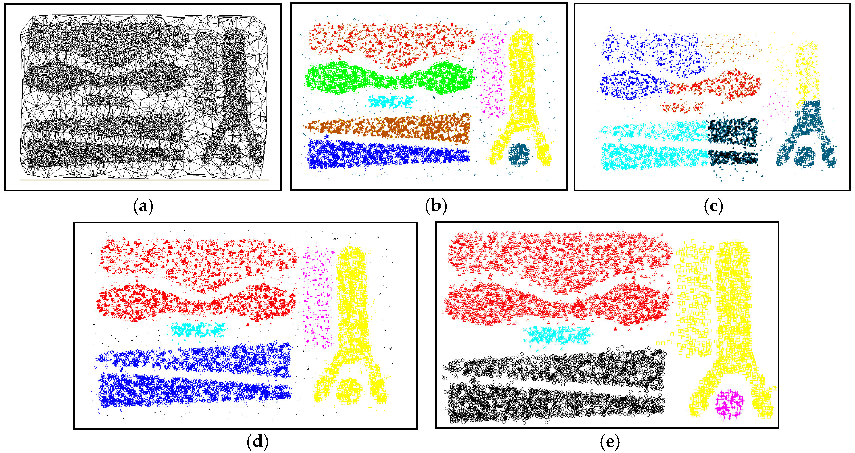
D1 includes 8000 points with eight arbitrary shape clusters of different densities and random noise as seen in Figure 11a. The DBSCAN, CURE and Žalik’s sweep-line algorithm (from here on referred to simply as “Žalik”) were all compared with the ASC. For the DBSCAN, MinPts was set to 4; Eps was fixed to 5.4; the shrink factor of CURE was set to 0.3; and the number of representative points was set to 12. Parameter d was set to 12 for the Žalik algorithm. The ASC algorithm automatically discovered arbitrary shapes, clusters of different densities and nested clusters (Figure 11b). It not only effectively detected all eight clusters but also correctly identified the noise in D1. The CURE algorithm was unable to identify spatial clusters with complex shape and incorrectly defined less dense spatial data as noise. The DBSCAN algorithm could not readily adapt to the density variations among clusters, while the Žalik algorithm used global parameters that prevented it from identifying clusters with varying densities.
There were 10,000 points in data set D2 (Figure 12). We varied the scaling factor , which causes changes in the threshold in order to form clusters at different hierarchies. The results demonstrated that a larger number of clusters were created if the threshold was small when was small. Conversely, the threshold was large if was large, resulting in a smaller number of clusters forming (i.e., relatively shallow hierarchy). When the value of is close to 1, clusters are easily and accurately distinguished from noise. In fact, the two effects create a favorable balance. These implicit hierarchical relationships with different thresholds related to are often used as the basis for analysis in practice [16].
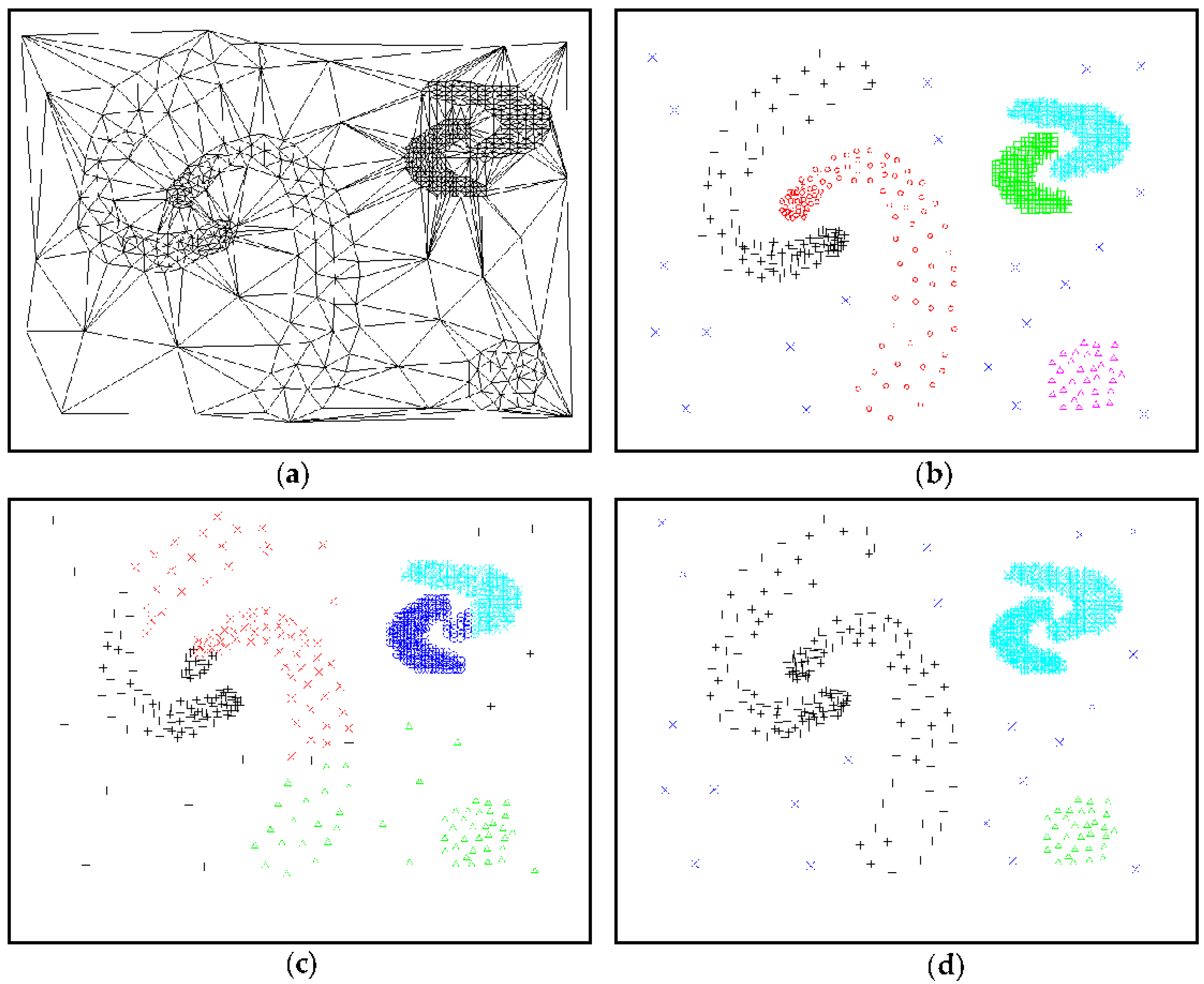
Data set D3 containing 264 test points was used to test the recognition effectiveness of the ASC algorithm in clusters with uneven internal densities and non-uniform data distribution. The clustering results of D3 by K-Means, DBSCAN (Minpts = 4 and Eps = 0.78), AMOEBA, Žalik (d = 0.0074) and the ASC algorithm are seen in Figure 13, which showed that the ASC algorithm was most suitable in discovering clusters of uneven internal density. The clusters were simply divided into several parts by K-Means, while DBSCAN detected noise accurately but failed to separate nearby clusters. Both the AMOEBA and the Žalik failed to identify clusters of uneven internal density.
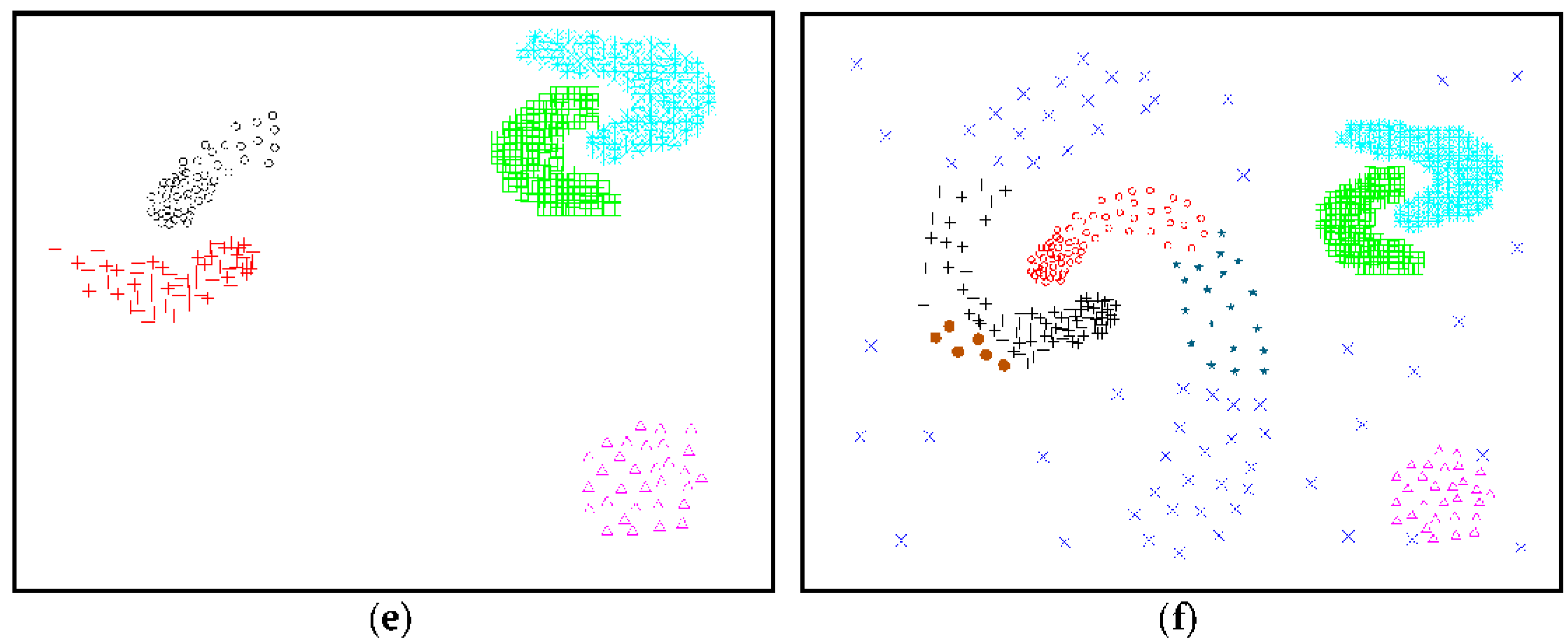
To illustrate the practical adaptability of ASC, we applied it to a real-world GIS data set collected obtained from the DCW (Digital Chart of the World), which focused on 15,067 position data points taken from Chinese cities, towns and villages pertaining to the population in 2002. The results from the ASC showed that the algorithm adapted well and is effective for this manner of practical application (See Figure 14).
5.3. CPU Time
The actual computational time for data processing is a greater concern in real-world applications, so we tested the proposed algorithm and compared it to several other methods accordingly. All algorithms were executed with the same development language, development environment, operating system and hardware (Intel R-core i3-3220 [email protected] 3.29 GHz and 2 GB memory, Seagate SV35 7200 rpm and access time 14.7 ms).
5.3.1. CPU Time Spent for Clustering
The CPU time spent for clustering data sets from Figure 11, Figure 12, Figure 13 and Figure 14 is compared in Table 2. The actual efficiency of CPU time is correlated to the number of clusters and test points generated. More CPU time was spent on larger numbers of clusters when the number of test points were the same. When the same number of clusters was obtained, the computational time decreased when there were fewer test points. Additional time was spent when clustering or merging many small clusters rather than one larger cluster.
Most current adaptive algorithms (AMOEB and AUTOCLUST) were developed based on the Delaunay triangulation (i.e., high spatial proximity). Table 3 shows a comparison of the traditional adaptive method AUTOCLUST against the proposed algorithm. AUTOCLUST is a relatively new algorithm developed to manage complex data sets (such as those with clusters of varying density and arbitrary shapes). This algorithm is similar to the proposed algorithm in that it can adaptively discover spatial clusters without the need to set parameters in advance. The implementation class of AUTOCLUST can be obtained from the Web [29].
There are several methods available for constructing Delaunay triangulations. We used the fastest Sweep Line (SL) algorithm according to the literature [35]. The experimental results suggested that ASC is more efficient than AUTOCLUST (Table 3). AUTOCLUST required more CPU time for Delaunay triangulation phase of the algorithm in addition to when dealing with repeated global and local uninteresting edges during the clustering process when the number of edges exceeded the number of points.
The CPU time spent between Žalik and ASC was compared (Table 4) using the same dataset, although different corresponding phases of the ASC algorithm were used. Initialization involved sorting input points by Quicksort in Žalik, which accounted for 22% of the total time spent. Initialization involved calculating the polar coordinate with Quicksort in ASC, which accounted for 30% of the total time. ASC employed the hash-table to speed up the efficiency during the clustering and merging phases when searching the event queue and locations on the borders. It was not necessary to consider projections that surpassed the border. However, this portion of the computational time in Žalik was spent both on missed projections and deleting the useless AF. In ASC, 8–9% of the total time was spent calculating polar coordinates of the input points and adaptive thresholds of the event points. Overall, there was less computational time and it is possible that the ASC algorithm could be truncated even further if the polar coordinates of the input points are obtained in advance.
5.3.2. CPU Time Spent for ASC-Based Stream Clustering
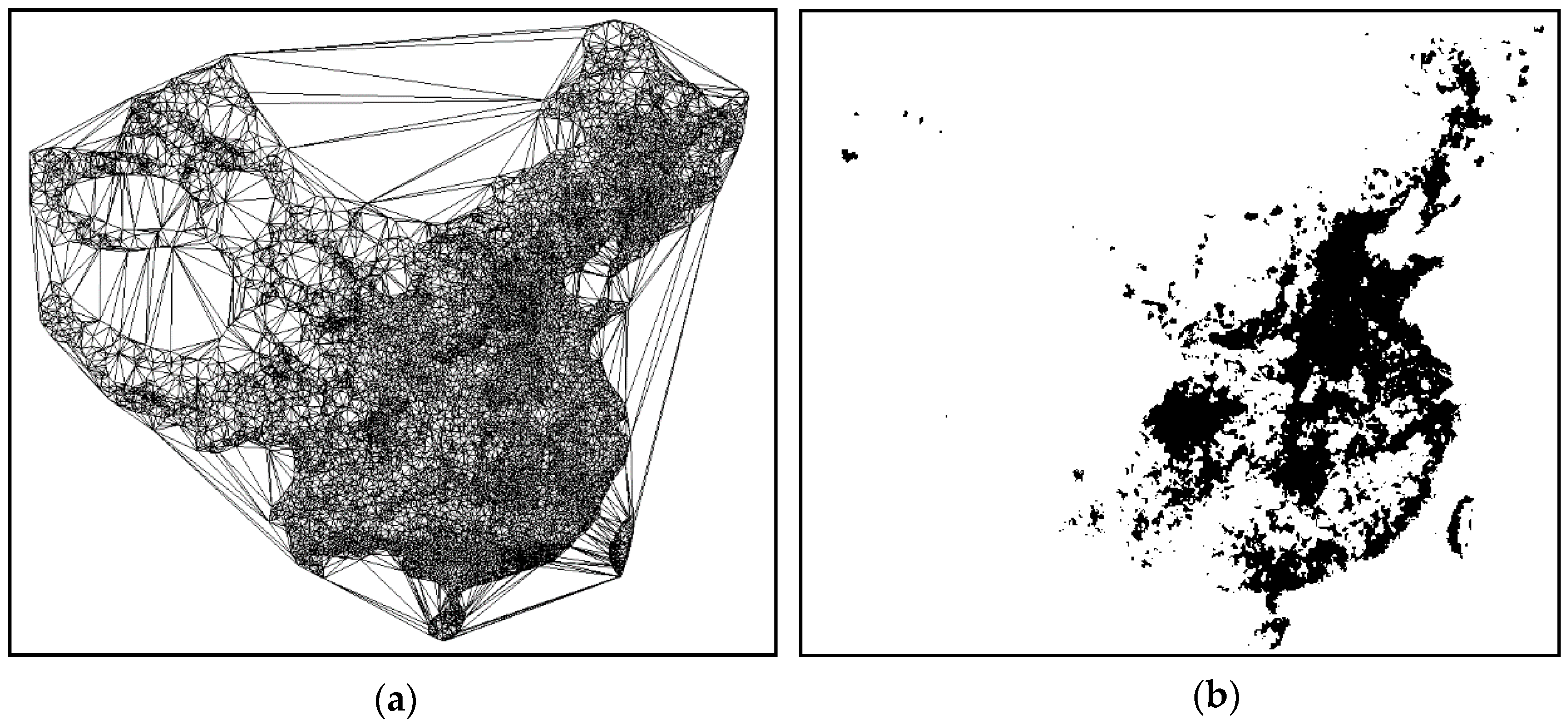
The ASC algorithm was also tested based on stream clustering techniques. Input spatial data sets were generated with high-resolution images obtained from Bing Maps (http://www.bing.com/maps/) containing 1.3 GB of data points. As shown in Figure 15, varying thresholds for (e.g., 100–600 m) and clusters K (e.g., 100–500) were provided to test the CPU time spent running the algorithm. The obtained clusters decreased with an increase in , while the running time of the algorithm was lower in the offline phase. Furthermore, having an value in the range of 100–300 resulted in relatively accurate clusters as shown in Figure 15. It required a longer period of time to generate a larger number of adaptive sub-clusters during the online phase.
6. Practical Applications of ASC
In order to explore the feasibility of the ASC algorithm in real-world scenarios, it was used to forecast geological disasters and quake magnitude based on geography. The real-world spatial data set containing 1264 geological disaster spots in Congzuo was collected from the geologic hazard database at the land department of Guangxi Zhuang Autonomous Region, China. The clustering results are shown in Figure 16.
ASC successfully detected nine clusters with varying densities within the disaster spots, which were divided into a preliminary distribution range of disaster-prone geographical areas (Figure 16c). It is possible to set a specific threshold (e.g., = 1000 m) in order to find areas that are most prone to major disasters, which could be beneficial for early warning purposes (Figure 16d).
7. Conclusions
The most notable conclusions of this study can be summarized as follows:
- The Gestalt theory was successfully applied to enhance the adaptability of the spatial clustering algorithm. Both the sweep-circle technique and the dynamic threshold setting was employed to detect spatial clusters.
- The ASC algorithm can automatically locate clusters in a single pass, rather than through modifying the initial model (i.e., via minimal spanning tree, Delaunay triangulation or Voronoi diagram). The algorithm could quickly adapt to identify arbitrarily-shaped clusters and could locate the non-homogeneous density characteristics of spatial data without necessitating a priori knowledge or parameters. The time complexity of the ASC algorithm was approximately O (nlogn), where n is the size of the spatial database.
- Scalability in ASC was not limited to the size of the data set, which demonstrated that the algorithm is suitable for data streaming technology to cluster large, dynamic spatial data sets.
- The proposed algorithm was efficient, feasible, easily understood and easily implemented.
The vast amount of information contained in spatial data sets and their relative complexity represent challenges that are yet to be solved. In the future, we believe we may benefit from further exploiting the characteristics of human vision. Humans can easily form clusters connected by chains and/or necks in addition to creating Gaussian clusters [14]. However, ASC is unable to discover these special clusters. Additionally, in ASC, points that do not belong to any cluster are treated as outliers/noise, where multiple outliers or noise points could be processed as new, independent clusters. Finally, the algorithm can potentially be extended to clustering spatial data with a higher dimensionality than those discussed in the present study.
Acknowledgments
This work has been supported by the National Science and Technology Support Program (Grant No. 2014BAL05B07) funded by the Ministry of Science and Technology of China.
Author Contributions
Qingming Zhan and Shuguang Deng conceived and designed the experiments; Shuguang Deng performed the experiments; All the authors analyzed the data; Qingming Zhan and Shuguang Deng wrote the paper. All authors contributed to revising the manuscript.
Conflicts of Interest
The authors declare no conflict of interest.
References
- Han, J.; Kamber, M.; Pei, J. Data Mining, 3rd ed.; Morgan Kaufmann: Boston, MA, USA, 2012. [Google Scholar]
- Chen, J.; Lin, X.; Zheng, H.; Bao, X. A novel cluster center fast determination clustering algorithm. Appl. Soft Comput. 2017, 57, 539–555. [Google Scholar]
- Deng, M.; Liu, Q.; Cheng, T.; Shi, Y. An adaptive spatial clustering algorithm based on Delaunay triangulation. Comput. Environ. Urban Syst. 2011, 35, 320–332. [Google Scholar] [CrossRef]
- Liu, Q.; Deng, M.; Shi, Y. Adaptive spatial clustering in the presence of obstacles and facilitators. Comput. Geosci. 2013, 56, 104–118. [Google Scholar] [CrossRef]
- Bouguettaya, A.; Yu, Q.; Liu, X.; Zhou, X.; Song, A. Efficient agglomerative hierarchical clustering. Expert Syst. Appl. 2015, 42, 2785–2797. [Google Scholar] [CrossRef]
- MacQueen, J. Some Methods for Classification and Analysis of Multivariate Observations. In Proceedings of the Fifth Berkeley Symposium on Mathematical Statistics and Probability, Berkeley, CA, USA, 21 June–18 July 1965 and 27 December 1965–7 January 1966; pp. 281–297. [Google Scholar]
- Ng, R.T.; Han, J. Efficient and effective clustering methods for spatial data mining. In Proceedings of the 20th International Conference on Very Large Data Bases, Santiago de Chile, Chile, 12–15 September 1994; pp. 144–155. [Google Scholar]
- Guha, S.; Rastogi, R.; Shim, K. Cure: An efficient clustering algorithm for large databases. Inf. Syst. 1998, 26, 35–58. [Google Scholar] [CrossRef]
- Zhang, T. Birch: An efficient data clustering method for very large databases. In Proceedings of the 1996 ACM SIGMOD international conference on Management of data, Montreal, QC, Canada, 4–6 June 1999; pp. 103–114. [Google Scholar]
- Karypis, G.; Han, E.-H.; Kumar, V. Chameleon: Hierarchical clustering using dynamic modeling. Computer 1999, 32, 68–75. [Google Scholar] [CrossRef]
- Ester, M.; Kriegel, H.-P.; Sander, J.; Xu, X. A density-based algorithm for discovering clusters in large spatial databases with noise. In Proceedings of the 2nd International Conference on Knowledge Discovery and Date Mining, Portland, OR, USA, 2–4 August 1996; pp. 226–231. [Google Scholar]
- Ankerst, M.; Breunig, M.M.; Kriegel, H.-P.; Sander, J. Optics: Ordering points to identify the clustering structure. In Proceedings of the 1999 ACM SIGMOD International Conference on Management of Data, Philadelphia, PA, USA, 31 May–3 June 1999; pp. 49–60. [Google Scholar]
- Hinneburg, A.; Keim, D.A. An Efficient Approach to Clustering in Large Multimedia Databases with Noise. In Proceedings of the 4th International Conference on Knowledge Discovery and Data Mining, New York, NY, USA, 27–31 August 1998; pp. 58–65. [Google Scholar]
- Zahn, C.T. Graph-theoretical methods for detecting and describing gestalt clusters. IEEE Trans. Comput. 1971, C-20, 68–86. [Google Scholar] [CrossRef]
- Estivill-Castro, V.; Lee, I. Autoclust: Automatic clustering via boundary extraction for mining massive point-data sets. In Proceedings of the 5th International Conference on Geocomputation, London, UK, 23–25 August 2000. [Google Scholar]
- Kang, I.-S.; Kim, T.-W.; Li, K.-J. A spatial data mining method by delaunay triangulation. In Proceedings of the 5th ACM International Workshop on Advances in Geographic Information Systems, Las Vegas, NV, USA, 10–14 November 1997; pp. 35–39. [Google Scholar]
- Wang, W.; Yang, J.; Muntz, R.R. Sting: A statistical information grid approach to spatial data mining. In Proceedings of the 23rd International Conference on Very Large Data Bases, Athens, Greece, 25–29 August 1997; pp. 186–195. [Google Scholar]
- Sheikholeslami, G.; Chatterjee, S.; Zhang, A. Wavecluster: A multi-resolution clustering approach for very large spatial databases. In Proceedings of the 24rd International Conference on Very Large Data Bases, New York, NY, USA, 24–27 August 1998; pp. 428–439. [Google Scholar]
- Dempster, A.P.; Laird, N.M.; Rubin, D.B. Maximum likelihood from incomplete data via the em algorithm. J. R. Stat. Soc. Ser. B 1977, 39, 1–38. [Google Scholar]
- Gennari, J.H.; Langley, P.; Fisher, D. Models of incremental concept formation. Artif. Intell. 1989, 40, 11–61. [Google Scholar] [CrossRef]
- Kohonen, T. Self-organized formation of topologically correct feature maps. Biol. Cybern. 1982, 43, 59–69. [Google Scholar] [CrossRef]
- Schikuta, E. Grid-clustering: An efficient hierarchical clustering method for very large data sets. In Proceedings of the 13th International Conference on Pattern Recognition, Vienna, Austria, 25–29 August 1996; pp. 101–105. [Google Scholar]
- Pei, T.; Zhu, A.X.; Zhou, C.; Li, B.; Qin, C. A new approach to the nearest-neighbour method to discover cluster features in overlaid spatial point processes. Int. J. Geogr. Inf. Sci. 2006, 20, 153–168. [Google Scholar] [CrossRef]
- Tsai, C.-F.; Tsai, C.-W.; Wu, H.-C.; Yang, T. Acodf: A novel data clustering approach for data mining in large databases. J. Syst. Softw. 2004, 73, 133–145. [Google Scholar] [CrossRef]
- Estivill-Castro, V.; Lee, I. Amoeba: Hierarchical clustering based on spatial proximity using delaunaty diagram. In Proceedings of the 9th International Symposium on Spatial Data Handling, Beijing, China, 10–12 August 2000. [Google Scholar]
- Estivill-Castro, V.; Lee, I. Argument free clustering for large spatial point-data sets via boundary extraction from delaunay diagram. Comput. Environ. Urban Syst. 2002, 26, 315–334. [Google Scholar] [CrossRef]
- Wei, C.P.; Lee, Y.H.; Hsu, C.M. Empirical comparison of fast partitioning-based clustering algorithms for large data sets. Expert Syst. Appl. 2003, 24, 351–363. [Google Scholar] [CrossRef]
- Li, D.; Yang, X.; Cui, W.; Gong, J.; Wu, H. A novel spatial clustering algorithm based on Delaunay triangulation. In Proceedings of the International Conference on Earth Observation Data Processing and Analysis (ICEODPA), Wuhan, China, 28–30 December 2008; Volume 7285, pp. 728530–728539. [Google Scholar]
- Liu, D.; Nosovskiy, G.V.; Sourina, O. Effective clustering and boundary detection algorithm based on delaunay triangulation. Pattern Recognit. Lett. 2008, 29, 1261–1273. [Google Scholar] [CrossRef]
- Nosovskiy, G.V.; Liu, D.; Sourina, O. Automatic clustering and boundary detection algorithm based on adaptive influence function. Pattern Recognit. 2008, 41, 2757–2776. [Google Scholar] [CrossRef]
- Xu, D.; Tian, Y. A comprehensive survey of clustering algorithms. Ann. Data Sci. 2015, 2, 165–193. [Google Scholar] [CrossRef]
- Zhao, Q.; Shi, Y.; Liu, Q.; Fränti, P. A grid-growing clustering algorithm for geo-spatial data. Pattern Recognit. Lett. 2015, 53, 77–84. [Google Scholar] [CrossRef]
- Bolaños, M.; Forrest, J.; Hahsler, M. Clustering large datasets using data stream clustering techniques. In Data Analysis, Machine Learning and Knowledge Discovery; Spiliopoulou, M., Schmidt-Thieme, L., Janning, R., Eds.; Springer International Publishing: Cham, Switzerland, 2014; pp. 135–143. [Google Scholar]
- Preparata, F.P.; Ian, S.M. Computational geometry: An Introduction; Springer-Verlag New York: New York, NY, USA, 1985. [Google Scholar]
- Žalik, B. An efficient sweep-line delaunay triangulation algorithm. Comput.-Aided Des. 2005, 37, 1027–1038. [Google Scholar] [CrossRef]
- Alfred, U. A mathematician’s progress. Math. Teach. 1966, 59, 722–727. [Google Scholar]
- Shamos, M.I.; Hoey, D. Geometric intersection problems. In Proceedings of the 17th Annual Symposium on Foundations of Computer Science, Houston, TX, USA, 25–27 October 1976; pp. 208–215. [Google Scholar]
- Bentley, J.L.; Ottmann, T.A. Algorithms for reporting and counting geometric intersections. IEEE Trans. Comput. 1979, C-28, 643–647. [Google Scholar] [CrossRef]
- Fortune, S. A sweepline algorithm for voronoi diagrams. Algorithmica 1987, 2, 153–174. [Google Scholar] [CrossRef]
- Zhou, P. Computational geometry algorithm design and analysis. In Computational Geometry Algorithm Design and Analysis, 4th ed.; Tsinghua University Press: Beijing, China, 2011. [Google Scholar]
- Žalik, K.R.; Žalik, B. A sweep-line algorithm for spatial clustering. Adv. Eng. Softw. 2009, 40, 445–451. [Google Scholar] [CrossRef]
- Biniaz, A.; Dastghaibyfard, G. A faster circle-sweep delaunay triangulation algorithm. Adv. Eng. Softw. 2012, 43, 1–13. [Google Scholar] [CrossRef]
- Adam, B.; Kauffmann, P.; Schmitt, D.; Spehner, J.-C. An increasing-circle sweep-algorithm to construct the Delaunay diagram in the plane. In Proceedings of the 9th Canadian Conference on Computational Geometry (CCCG), Kingston, ON, Canada, 11–14 August 1997. [Google Scholar]
- Guha, S.; Mishra, N.; Motwani, R.; O’Callaghan, L. Clustering data streams. In Proceedings of the 41st Annual Symposium on Foundations of Computer Science, Redondo Beach, CA, USA, 12–14 November 2000; pp. 359–366. [Google Scholar]
- O’Callaghan, L.; Mishra, N.; Meyerson, A.; Guha, S.; Motwani, R. Streaming-data algorithms for high-quality clustering. In Proceedings of the 18th International Conference on Data Engineering, San Jose, CA, USA, 26 February–1 March 2002; pp. 685–694. [Google Scholar]
- Zengyou, H.E.; Xiaofei, X.U.; Deng, S. Squeezer: An efficient algorithm for clustering categorical data. J. Comput. Sci. Technol. 2002, 17, 611–624. [Google Scholar]
- Guha, S.; Meyerson, A.; Mishra, N.; Motwani, R.; O’Callaghan, L. Clustering data streams: Theory and practice. IEEE Trans. Knowl. Data Eng. 2003, 15, 515–528. [Google Scholar] [CrossRef]
- Ding, S.; Zhang, J.; Jia, H.; Qian, J. An adaptive density data stream clustering algorithm. Cogn. Comput. 2016, 8, 30–38. [Google Scholar] [CrossRef]
- Zheng, L.; Huo, H.; Guo, Y.; Fang, T. Supervised adaptive incremental clustering for data stream of chunks. Neurocomputing 2016, 219, 502–517. [Google Scholar] [CrossRef]
- Tobler, W.R. A computer movie simulating urban growth in the detroit region. Econ. Geogr. 1970, 46, 234–240. [Google Scholar] [CrossRef]
- Ellis, W.D. A Source Book of Gestalt Psychology; Kegan Paul, Trench, Trubner & Company: London, UK, 1938; p. 403. [Google Scholar]
- Hathaway, R.J.; Bezdek, J.C. Extending fuzzy and probabilistic clustering to very large data sets. Comput. Stat. Data Anal. 2006, 51, 215–234. [Google Scholar] [CrossRef]
- Cho, K.; Jo, S.; Jang, H.; Kim, S.M.; Song, J. Dcf: An efficient data stream clustering framework for streaming applications. In Proceedings of the 17th International Conference on Database and Expert Systems Applications, Kraków, Poland, 4–8 September 2006; pp. 114–122. [Google Scholar]
Figure 1.
Incremental sweep circle algorithm used to construct Delaunay triangulation.

Figure 2.
Sweeping the points by the sweep-lines.

Figure 3.
Sweeping the data set to obtain clusters.

Figure 4.
Initial frontier.

Figure 5.
Grouping principles with regards to: (a) proximity; (b) continuity; and (c) closure.

Figure 6.
Grouping principles exemplified.

Figure 7.
Adaptive dynamic threshold example.

Figure 8.
Adaptive spatial clustering (ASC) algorithm cluster basics with the following steps: (a) sweeping of the points; and (b) obtaining two clusters.
Figure 8.
Adaptive spatial clustering (ASC) algorithm cluster basics with the following steps: (a) sweeping of the points; and (b) obtaining two clusters.

Figure 9.
Hash-table on a circular double-linked list for sweep-circle clustering.

Figure 10.
Vertexes located on the same line.

Figure 11.
Testing data set D1 of ASC: (a) Graph built by triangulation of D1; (b) clustering result by ASC; (c) clustering result by DBSCAN; (d) clustering result by CURE; and (e) clustering result by Žalik.
Figure 11.
Testing data set D1 of ASC: (a) Graph built by triangulation of D1; (b) clustering result by ASC; (c) clustering result by DBSCAN; (d) clustering result by CURE; and (e) clustering result by Žalik.

Figure 12.
Results largely dependent on parameters: (a) Graph built by triangulation of D2; (b) 20 clusters obtained when = 1; (c) 30 clusters obtained when = 0.8; and (d) 8 clusters obtained when = 1.2.
Figure 12.
Results largely dependent on parameters: (a) Graph built by triangulation of D2; (b) 20 clusters obtained when = 1; (c) 30 clusters obtained when = 0.8; and (d) 8 clusters obtained when = 1.2.

Figure 13.
Clustering results of data set D3 by comparison: (a) Graph built by triangulation of D3; (b) clustering result by ASC; (c) clustering result by K-Means; (d) clustering result by DBSCAN; (e) clustering result by Žalik; and (f) clustering result by AMOEBA.
Figure 13.
Clustering results of data set D3 by comparison: (a) Graph built by triangulation of D3; (b) clustering result by ASC; (c) clustering result by K-Means; (d) clustering result by DBSCAN; (e) clustering result by Žalik; and (f) clustering result by AMOEBA.


Figure 14.
Clusters discovered by ASC in large spatial datasets: (a) graph built by triangulation of GIS datasets; and (b) clustering results of GIS large spatial datasets generated by ASC.
Figure 14.
Clusters discovered by ASC in large spatial datasets: (a) graph built by triangulation of GIS datasets; and (b) clustering results of GIS large spatial datasets generated by ASC.

Figure 15.
Speed comparison of stream clustering.

Figure 16.
Spatial clustering results for disaster database by ASC: (a) Distribution of disaster data points; (b) description of spatial neighborhood relations via Delaunay triangulation; (c) clustering result of ASC; and (d) clustering result of user-defined threshold setting ( = 1000 m).
Figure 16.
Spatial clustering results for disaster database by ASC: (a) Distribution of disaster data points; (b) description of spatial neighborhood relations via Delaunay triangulation; (c) clustering result of ASC; and (d) clustering result of user-defined threshold setting ( = 1000 m).


Table 1.
Comparisons of some classical spatial clustering algorithms.
| Category | Typical Algorithm | Shape of Suitable Data Set | Discovery of Clusters with Even Density | Scalability | Requirement of Prior Knowledge | Sensitive to Noise/Outlier | for Large-Scale Data | Complexity (Times) |
|---|---|---|---|---|---|---|---|---|
| Partition | K-means | Convex | No | Middle | Yes | Highly | Yes | Low |
| CLARANS | Convex | No | Middle | Yes | Little | Yes | High | |
| Hierarchy | BIRCH | Convex | No | High | Yes | Little | Yes | Low |
| CURE | Arbitrary | No | High | Yes | Little | Yes | Low | |
| CHAMELEON | Arbitrary | Yes | High | Yes | Little | No | High | |
| Density | DBSCAN | Arbitrary | No | Middle | Yes | Little | Yes | Middle |
| OPTICS | Arbitrary | Yes | Middle | Yes | Little | Yes | Middle | |
| DENCLUE | Arbitrary | No | Middle | Yes | Little | Yes | Middle | |
| Graph theory | MST | Arbitrary | Yes | High | Yes | Highly | Yes | Middle |
| AMEOBA | Arbitrary | Yes | High | No | Little | No | Middle | |
| AUTOCLUST | Arbitrary | Yes | High | No | Little | No | Middle | |
| Grid | STING | Arbitrary | No | High | Yes | Little | Yes | Low |
| CLIQUE | Arbitrary | No | High | Yes | Moderately | No | Low | |
| WaveCluster | Arbitrary | No | High | Yes | Little | Yes | Low | |
| Model | EM | Convex | No | Middle | Yes | Highly | No | Low |
Table 2.
CPU time (s) spent for clustering.
| Data Set | Points | CPU Time (s) |
|---|---|---|
| Figure 13 | 264 | 0.014 |
| Figure 11 | 8000 | 0.074 |
| Figure 12b | 10,000 | 0.116 |
| Figure 12c | 10,000 | 0.124 |
| Figure 12d | 10,000 | 0.243 |
| Figure 14 | 15,067 | 0.457 |
Table 3.
CPU time (s) spent by ASC and AUTOCLUST for clustering.
| Dataset | ASC | AUTOCLUST | ||
|---|---|---|---|---|
| Clustering Time | DT Time | Clustering Time | Total (s) | |
| 10,000 | 0.249 | 0.026 | 0.314 | 0.340 |
| 20,000 | 0.422 | 0.082 | 2.450 | 2.532 |
| 50,000 | 0.941 | 0.287 | 5.125 | 5.412 |
| 100,000 | 2.653 | 0.607 | 14.234 | 14.841 |
| 200,000 | 5.324 | 2.290 | 61.124 | 63.414 |
Table 4.
CPU time (s) spent by ASC and Žalik for different algorithm phases.
| Data Set Algorithm | 100,000 | 200,000 | ||
|---|---|---|---|---|
| ASC | Žalik | ASC | Žalik | |
| Initialization | 0.646 | 0.717 | 1.597 | 2.700 |
| Clustering | 1.026 | 1.944 | 2.715 | 7.242 |
| Merging | 0.481 | 0.624 | 1.012 | 2.332 |
| Total | 2.153 | 3.285 | 5.324 | 12.274 |
© 2017 by the authors. Licensee MDPI, Basel, Switzerland. This article is an open access article distributed under the terms and conditions of the Creative Commons Attribution (CC BY) license (http://creativecommons.org/licenses/by/4.0/).
Share and Cite
MDPI and ACS Style
Zhan, Q.; Deng, S.; Zheng, Z. An Adaptive Sweep-Circle Spatial Clustering Algorithm Based on Gestalt. ISPRS Int. J. Geo-Inf. 2017, 6, 272. https://doi.org/10.3390/ijgi6090272
AMA Style
Zhan Q, Deng S, Zheng Z. An Adaptive Sweep-Circle Spatial Clustering Algorithm Based on Gestalt. ISPRS International Journal of Geo-Information. 2017; 6(9):272. https://doi.org/10.3390/ijgi6090272
Chicago/Turabian StyleZhan, Qingming, Shuguang Deng, and Zhihua Zheng. 2017. "An Adaptive Sweep-Circle Spatial Clustering Algorithm Based on Gestalt" ISPRS International Journal of Geo-Information 6, no. 9: 272. https://doi.org/10.3390/ijgi6090272
Note that from the first issue of 2016, this journal uses article numbers instead of page numbers. See further details here.