Hybrid 3D Rendering of Large Map Data for Crisis Management

Abstract

In this paper we investigate the use of games technologies for the research and the development of 3D representations of real environments captured from GIS information and open source map data. Challenges involved in this area concern the large data-sets to be dealt with. Some existing map data include errors and are not complete, which makes the generation of realistic and accurate 3D environments problematic. The domain of application of our work is crisis management which requires very accurate GIS or map information. We believe the use of creating a 3D virtual environment using real map data whilst correcting and completing the missing data, improves the quality and performance of crisis management decision support system to provide a more natural and intuitive interface for crisis managers. Consequently, we present a case study into issues related to combining multiple large datasets to create an accurate representation of a novel, multi-layered, hybrid real-world maps. The hybrid map generation combines LiDAR, Ordnance Survey, and OpenStreetMap data to generate 3D cities spanning 1 km². Evaluation of initial visualised scenes is presented. Initial tests consist of a 1 km² landscape map containing up to 16 million vertices’ and run at an optimal 51.66 frames per-second.

1. Introduction

Creating detailed and realistic 3D virtual environments for real-world maps for crisis management applications is increasingly difficult due to the variety, complexity, and large-scale GIS datasets. Modern GIS visualisation applications focus on a limited number of datasets [1,2,3] with relation to crisis management. Combining multiple datasets can alleviate errors, produce unmapped areas, and increase accuracy of a map for terraforming of extruded models in runtime applications.

The creation of realistic virtual scenes at crisis time gives crisis managers the ability to plan specific emergency procedures: evacuations, fire extinguishing, flood prevention, etc. If errors or inaccurate data is visualised, the cascading effects can, and will, if not circumvented, cause vast upset and potential loss of life.

Map data including critical infrastructures’ are highly complex and include very large sets of data. For example, in the USA alone there are 560,104 infrastructures. In 2005, there were: two million miles of pipeline, 2800 power plants (with 300,000 production sites providing assets), 104 nuclear power plants, 80,000 dams, 60,000 chemical plants, 87,000 food-processing plants, 28,600 networked Federal Deposit Insurance Corporation institutions, and 1600 water-treatment plants [4]. If accidental, natural, or man-made upset happened to a single one of these infrastructures then this can have vast consequences and cascading effects to many other infrastructures of the USA. If crisis managers produce evacuation plans for specific infrastructures, the need for accurate, high resolution maps to create accurate recovery plans are needed. For instance, top-down 2D map representations do not give a fully immersive experience into the best locations for emergency vehicles to be placed. High resolution maps containing height points separated by small cell values give improved spatial awareness which is critical for the placing and manoeuvring of emergency vehicles.

In addition to map complexity, the map data is not always kept up to date timely. For example, Google’s map system can be up to three years out of date for highly populated areas, and further out of date for rural areas. Although the updating of commercial map data can be helped by using crowd-sourced data, as used with OpenStreetMap.org, this is not yet a common practice.

Current solutions provide limited user interaction, constricting a user’s ability to fully understand a scene, as discussed in Section 2.2. The use of modern commercial game engines can provide cheaper, or free, alternatives to custom bespoke pieces of software. Research in user-experience shows that immersion into simulations is broken, when inaccuracies, such as visible unsmooth level of detail (LOD) morphing, occurs [5]. Robertson et al. state that a common criticism of immersion is the lack of peripheral vision due to limited screen size [5]. Game engines can allow advanced immersion into 3D scenes with use of: common rendering algorithms, culling techniques to produce large scale scenes running in real-time, animation systems which can be built upon, and advanced mathematics modules used for 3D world navigation and 3D camera creation. Advanced camera systems are capable of real-time changeable perspectives and projections to aid a user’s interaction and understanding of a scene; perspective and orthographic projection. Perspective projection shows depth, orthographic [6,7]. Within this paper, we discuss the procedures and techniques needed to create novel hybrid maps, for 3D terrain and scene generation, from the use of big data fusion from several GIS data sources and procedural techniques. State-of-the-art rendering techniques for the visualisation of hybrid maps will be implemented by a commercial grade game engine specifically designed for crisis management. Light Detection and Ranging (LiDAR) [8,9,10], OpenStreetMap (OSM) [11], and Ordnance Survey (OS) [12] data are combined to reduce error and create increased accurate layered maps for use within a modern novel disaster support system using 3D environments. The layered hierarchy of maps allow a user to view the information they want to see; static or dynamic artefacts, highly detailed terrains, and procedurally generated content (PCG) [13,14,15,16], and specific infrastructure buildings. Uses of filtering and interpolation algorithms are used to correct errors and generate missing map data. See [17] for early work into interpolation techniques for derivative of digital elevation models. For our research we will focus on the use and implementation of Catmull-Rom interpolation [18,19].

The research focus is on map data generation, specifically the processes of combining maps in a variety of combinations, and the interpolation of data points.

The case study will test the improved high resolution map data within a game engine to decide the best resolution map density needed to run at a minimum 30 frames per-second.

The paper is structured as follows. Section 2 covers background work consisting of crisis management, related work and open data. Section 3 covers our visualisation framework and the techniques and procedures for the generation and combination of multiple map datasets. Section 4 discusses evaluations of the framework. Section 5 states future work. Section 6 concludes our discussion and paper.

2. Background

Within this section we will cover background research into crisis management and current state of the art visualisation tools and techniques focusing on terrain and map generation.

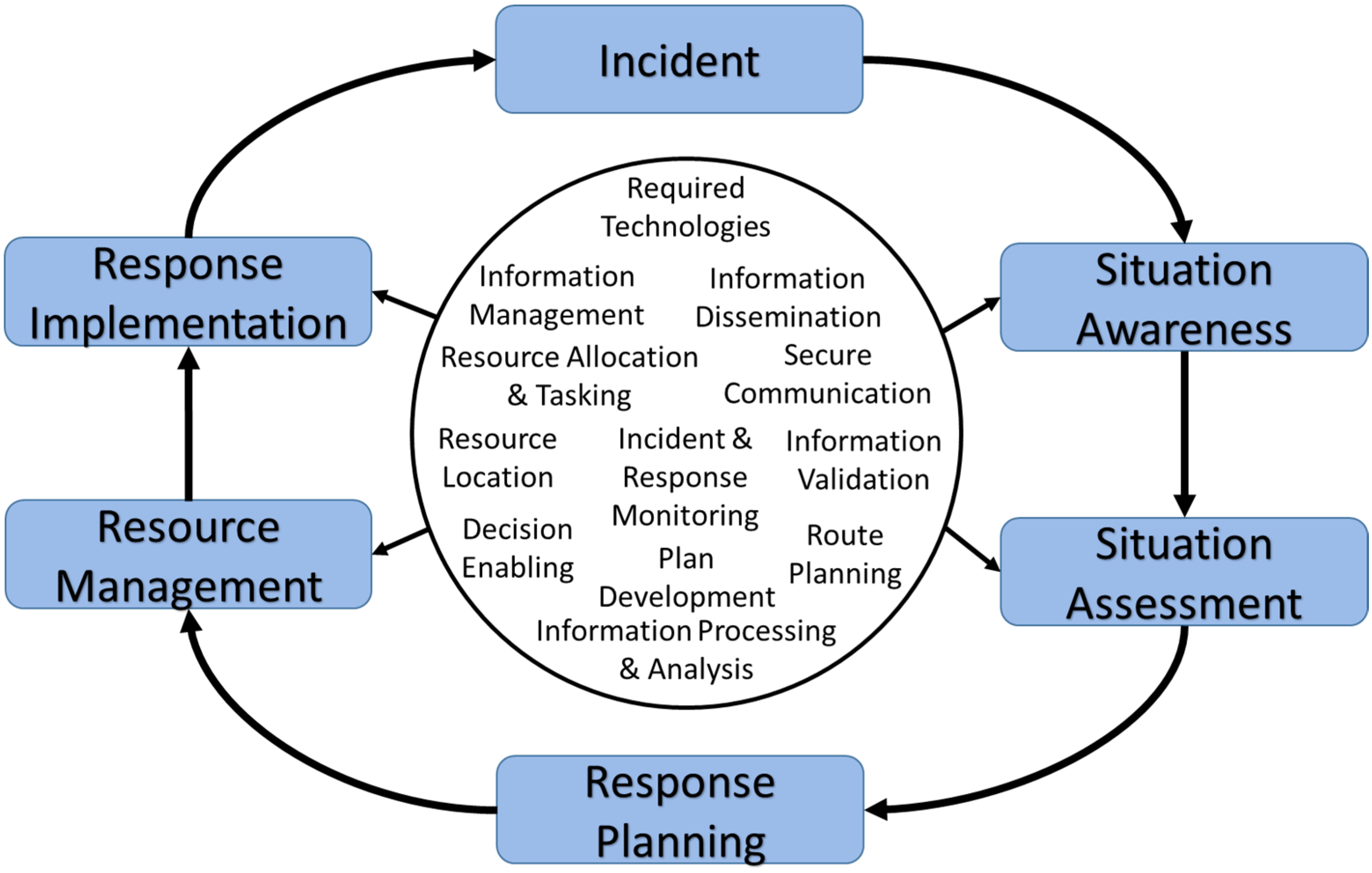
2.1. Crisis Management

Interdependencies between infrastructures and unforeseen non-natural disasters can bring cities to a standstill [20]. A clear demand for proactive and reactive management strategies and systems for severe critical infrastructure (CI) disasters are needed [21]. Currently, limited response and effectiveness of plans and systems are hindered by: large number and diversity of stakeholders; conflicting demands and resources; and the lack of cooperation between different stakeholders, despite the best efforts of communities and governments [20,21].

When a crisis incident occurs, response is a cyclic/iterative dynamic procedure. See Figure 1 for incident cycle.

Minimising decision time at crisis situation saves lives, resources, and costs. Fully understanding a large local area is time consuming. Many applications are available for the viewing of real-world scenes at crisis and non-crisis time. For example, Aqil et al. present a tool for real-time flood monitoring and simulation [22].

The application is limited to a top-down 2D representation of large areas giving little perspective to a scene/terrain. Simplistic polygon representations are used for flooded areas. Generation of realistic height terrains and 3D virtual cameras navigating scenes will produce a fuller understanding of potential flood plains, or potential flood paths; functionality that the Aqil et al. tool does not have.

We have observed from [23] that there are four types of interdependencies between infrastructures: Physical, Cyber, Geographical, and Logical. Within our research, we are focusing on the physical and geographical interdependencies due to their relevance to visualisation, and their impact on the constraints they inhibit on potential crisis management plans. For example, the physical dependencies between a coal mine and a power plant, connected by roads used for delivery, are put at risk if flooding of said roads prevents delivery.

Figure 1. Incident and crisis management response cycle.

Figure 1. Incident and crisis management response cycle.

To prevent this situation, crisis managers and city planners can generate virtual scenes within our visualisation framework, to simulate this situation. If map data is initially wrong, i.e., contains missing or inaccurate/outdated data, then user generated plans can be wrong from the beginning.

As highlighted, high complexity, inaccuracies, and incompleteness of map data; and lack of appropriate visualisation solutions, are all the challenges we meet in dealing with 3D rendering of large map data for crisis management.

In their paper, Kwan and Jiyeong [24] state the potential importance for real-time 3D GIS frameworks for quick emergency response. They present a GIS-based intelligent emergency response system (GIERS) that aims to visualize and detect potential bottle necks in conduits within environments and a focus on building structures for use of terrorist attacks on buildings.

To solve some of these problems and provide a more fitting solution, we put forward procedures, which will alleviate these issues by use of hybrid GIS data combination techniques and game technology visualisation techniques.

2.2. Related Work

In this section, we discuss the current state of the art in visualisation tools and techniques for geographical information.

Sketchaworld [25] is a tool that converts simplified sketches of landscapes, and generates full 2D and 3D procedural environments able to tackle rivers and bridges. The tool can generalise conflicting user inputs and create satisfactory scenes. This work does not include real world data, thus, the maps in question are user generated and subject to unrealistic terrain generation. Using real-world data with their procedural techniques will provide greater realism for future city planners. We would like to use this software as a benchmark for ideas into the interactivity and design procedures, which may be relevant to users in a decision support system for crisis management. For example, a user can input a shorter path between destinations for use in pathfinding algorithms [26,27,28,29,30], such as through parks or open spaces which vehicles are normally prohibited to travel, and see the effects it might have on the planning algorithms used for automated routing.

Tanagra [31] is an editing tool that uses a mixed initiative paradigm to create a tool which helps the creation of 2D platform levels. Objects are placed within the world, such as obstacles and platforms, which the player must navigate to get to the end of the level. They state current techniques in procedural level generation tend to offer little author guidance and suggest other techniques allowing them to tweak parameters and variables, which can be “unintuitive, with small shifts leading to radical changes in the produced content”. Mixed initiative is the term where user and algorithm work together to create content; the algorithm suggests the next position of objects in the world, and in some cases overrides the user’s decision because of unreachable desires. Using a mixed initiative approach provides access to large numbers of varying map types. A procedural autonomous map generator can ask a user to resolve conflicts of data within a scene. For example, if one data-set states land height should be above sea level, and another state below sea-level, the user can be queried.

Falconer et al. [32] created a prototype simulation and visualisation tool, named “SAVE”, which allows stakeholders to interact with a virtual environment composed of real-world data combing computer game technology with computer modelling techniques. Their work has been used to model effect and cause of future concepts and plans for the sustainability of assets within the environment, e.g., buildings, population, economy, etc. Their application colours assets, which the stakeholder is interested in, with distinctive colours and patterns representing high or low results for the effect they want to observe; sustainability, cost and safety comparisons, among others. Their tool needs a large number of user-generated variables representing their personal interest of assets. We want to use similar visualisation techniques to view scenes with multiple overlays, highlighting crisis situations, infrastructure critical buildings, and potential crisis zones.

A real-time procedurally generated, GPU only, application for the visualisation and interaction of real-time accurate fluid simulator has been created by Kellomäki [33]. We believe we can implement this purely GPU driven fluid simulator in our simulation and accurately model many scenarios involving water, with tremendous realism. The simulation can also interact with a physics engine to move objects within in a scene, simulating the damage a flood can create. The algorithm can also take into account rainfall data, which is specifically interesting to our work. Modelling the rainfall predicted by the METoffice, can simulate flash floods or even dam water levels and predict how long it will be before flooding commences. To observe accurate simulation of fluids within a scene, accurate terraforming of real-world map data is needed, otherwise, the fluid simulator will guide the resource in the wrong direction, with potential of huge consequences.

Autonomous Learning Agents for Decentralised Data and Information Network (ALADDIN), a research project to investigate multi-agent systems and data fusion, decision making, resource allocation, and other domains. The project consists of simple visualisations but complex planning procedures. An issue with this work is the limited visualisation of 2D scenes.

The SAVE project and ALADDIN project are great examples which we can be built upon with the use of 3D game technologies.

The commercial product CityEngine [34] created by ESRI, a GIS mapping software solution company, provides in-depth analysis into future city planning. The claim of generating a large city within five steps is impressive: (1) prepare 2D data/geodatabase, (2) import and edit city layout, (3) generate 3D building and streets, (4) texture facades, and (5) visualise and share 3D city models. Using preprocessing technique as discussed in future sections, we wish to streamline this process by combining the processes and only interacting with a user when an unresolvable conflict is encountered. The CityEngine also has the ability to visualise land use zoning of residential, and commercial areas for the help with future city planning and zoning law. We can adopt a similar technique for use by crisis managers and intelligent systems to organize and potentially avoid certain zoned areas such as residential areas at night for loud sirens, or avoid contaminated areas. Another commercial product, which can be used for benchmarking our system, is CyberCity3D [35], a city visualisation analysis system.

Visualisation is not the only problem with creating a coherent modern decision support system for crisis management. Correct and accurate data is key for successful planning for possible future issues.

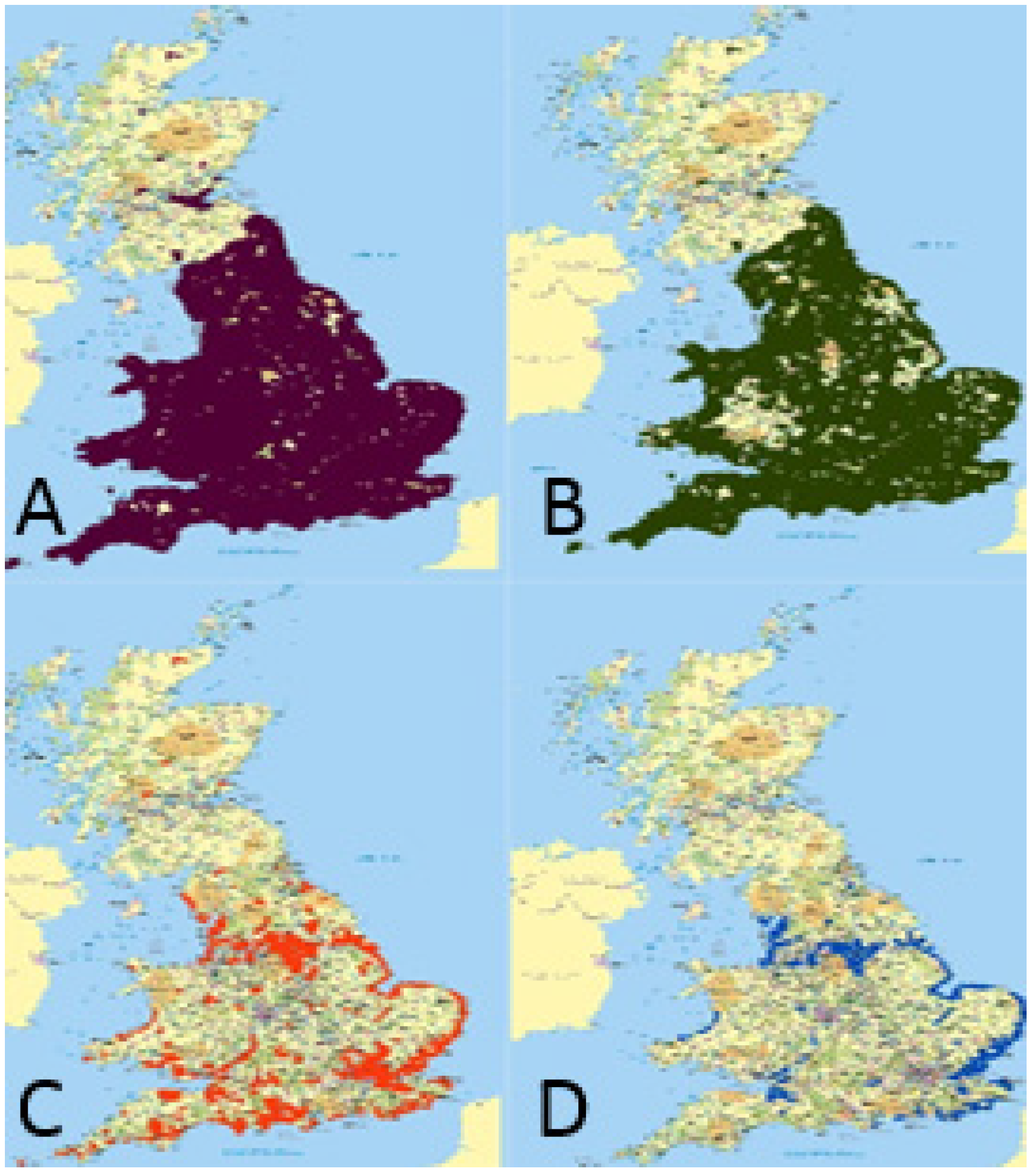
2.3. Digital Map Open Data

Open data is freely available, often through Internet portals, provided by companies and government sectors. Careful consideration must be given when working with open-data due to inconsistencies and quality assurance and amount of multiple data types and file formats.

Many projects have incorporated open data for improved visualisation and engagement: Open Data Monopoly; Bar Chart Ball [36]; Open Trumps; Flight Leader; Urbanopoly, MuseumVILLE, and Open Street Racer. For example, the Open Street Racer uses OSM data to generate virtual racing tracks through procedurally generated urban environments, translating buildings, which interrupt the track playability [37].

Combination of open data and commercial data can alleviate errors within single maps by querying each map to detect anomalies.

We propose to use a mixed initiative approach to content generation: procedurally generating landscapes and building models at multiple LOD at run-time will allow generalised map generation of many selected areas, and premade models of assets, which can be tailored offline and loaded when necessary. The use of LiDAR and OSM data will be the most relevant and accurate data sets for this type of content creation due to the high density of LiDAR data sets with the added minimum error rate of between 5–15 cm, and OSM for the ability for streamlined and ability to input custom data-tags which can be used directed by disaster support systems. OSM implements quality assurance procedures, by human and procedural operators, to minimize user-inputted error in the data sets. The use of OS data is needed as a base of interpolation, which will be used when no other accurate data, or data which can be interpolated, or derived from procedural techniques are available.

3. Visualisation Framework

This section we present our framework Project Vision Support (PVS), a multi-agent system which combines an advanced game engine and planning algorithms to manipulate complex intertwining sets of big-data extracted from real-world map instances, to aid the action planning of emergency services and response management during crisis events.

PVS is a C# framework built on top of a modern game engine [38]. We have upgraded the engine used for the framework to a more advanced version of DirectX [39]. As stated in [40], most CAD and GIS applications do not have the ability of 3D tools, navigation systems, and physics math libraries, whereas most games engines do, or can be extended with the use of freely available libraries. The framework includes many separate components as depicted in Figure 2. The main “engine” consists of: animation classes, custom 2D and 3D camera classes, debugging classes, primitive geometry classes, input systems, advanced shader classes used for advanced rendering, and advanced screen system. The main project extends these basic objects for custom assets such as buildings or road networks.

Figure 2. Project Vision Support Framework Components.

Figure 2. Project Vision Support Framework Components.

Figure 3. PVS procedural city generation of New York Manhattan containing buildings, roads, and rail networks.

Figure 3. PVS procedural city generation of New York Manhattan containing buildings, roads, and rail networks.

PVS has the ability to convert the OSM data and generate 3D environments including minimal procedural buildings (walls and roof tops), road networks, amenities (user generated assets, such as pharmacies and parking areas), as well as boundary locations used for depicting emergency locations. The power of PVS is the ability to generate procedural scenes from any OSM map selected from the OSM webpage. See Figure 3 to see an 800 m² visualisation of an area of New York Manhattan. A screen shot of Open Street Racer is shown in [37]. Open Street Racer generates procedural tracks but relocates generated buildings, which impact the track, producing inaccurate visualisations. Generated OSM buildings and road and rail networks are visualised to the unaltered OSM specifications in Figure 3. Object pooling allows the visualisation of large cities within the UK, currently tested up to 115 km² running above 50 frames per second (FPS).

In the following sections, we will focus on map data generation procedures and algorithms, specifically the data complexity, the generation of missing data, errors in data and related issues.

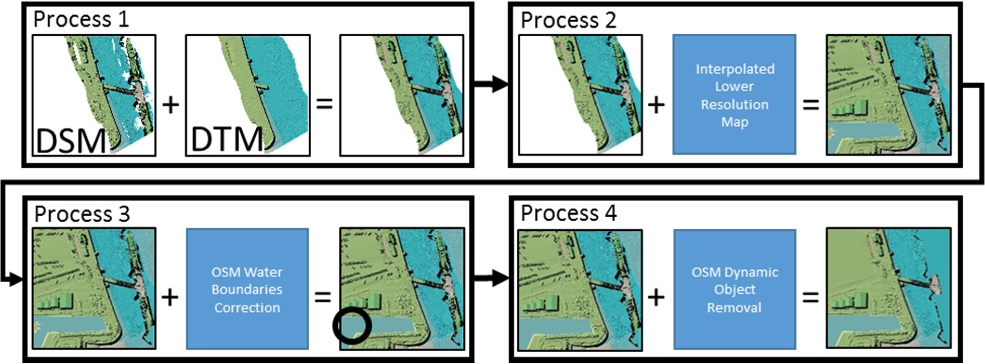
3.1. Map Data Generator

Generation of 3D terrains within virtual environments is a common technique in modern computer games. Generating real-world, accurate, terrains representing one kilometre square at multiple resolutions adds additional problems. Increased computation and memory consumption at runtime, and storage limits are issues, which need to be overcome.

Terrain meshes generated in games are traditionally created in square grids, with vertex points separated in equal segments, called cells. A map of 500² points at 2 m cells representing 1 km², will use 250,000 vertex points, containing data specific for each application: position in a 3D world, 1 or more texture coordinates, and quite often a facing vector direction for use with advanced lighting systems. Terrain generated at this resolution using real-world recordings, with cell sizes representing 2 meters apart, has the potential to miss vital information such as walls, trees, bollards, small buildings, and telephone boxes. Producing higher resolution maps by combining multiple GIS datasets can reduce this error.

Ordnance Survey (OS) Data is terrain height maps represented by points separated by 50 metres, covering the whole UK. This distance of 50 m² is a generalisation of the terrain heights above sea level recorded using Ordnance Datum Newlyn. Each map file covers 10 km² containing 200² points. A subset of 1km² map will contain only 20² points from the larger OS map. The potential for missed artefacts within a scene is vast. Although the data is only a generalisation, improvements can be made with the combination of alternative GIS datasets such as OSM and LiDAR data.

LiDAR is a mapping technique capable of recording highly accurate spatial positions on a surface. The LiDAR data obtained was captured by flying a small aircraft over selected areas, commonly at 800–1000 feet. Because of the high cost of flying an aircraft, much of the UK is unmapped. Where mapping has taken place, multiple resolutions are normally available. Figure 4 shows the areas of UK which has been mapped. Image A represents the areas of the UK which have been mapped to a 2 m resolution, image B represents 1 m resolution coverage, image C represents 0.5 m resolution coverage, and image D represents 0.25 m resolution coverage. See Table 1 to compare LiDAR resolution with area coverage and point density. Light pulses are shot towards the surface of the Earth, and sensors detect how long the light signal takes to bounce of the surface, back to the aircraft. As stated, this particular data is accurate to within 5–15 cm of error. The data provided is split into two types of map: Digital Terrain Model (DTM) and Digital Surface Model (DSM).

Figure 4. LiDAR coverage of the UK. (A) 2 m resolution, (B) 1 m resolution, (C) 0.5 m resolution, and (D) 0.25 m resolution.

Figure 4. LiDAR coverage of the UK. (A) 2 m resolution, (B) 1 m resolution, (C) 0.5 m resolution, and (D) 0.25 m resolution.

Table 1. LiDAR data comparison.

LiDAR Map	Area	Points Contained
2 m	1 km2	5002 = 250,000
1 m	1 km2	10002 = 1,000,000
0.5 m	500 m2	10002 = 1,000,000
0.25 m	500 m2	20002 = 4,000,000
Proposed 0.25 m	1 km2	40002 = 16,000,000

Table 1. LiDAR data comparison.

LiDAR Map	Area	Points Contained
2 m	1 km2	5002 = 250,000
1 m	1 km2	10002 = 1,000,000
0.5 m	500 m2	10002 = 1,000,000
0.25 m	500 m2	20002 = 4,000,000
Proposed 0.25 m	1 km2	40002 = 16,000,000

A DTM map is pre-processed interpolated data-set representing only the terrain height, removing all objects from a scene: buildings, trees, cars etc. interpolation only occurs when small areas of data is missing and is done by the company from whom we obtained the data from Geomatics-Group [8]. Figure 5 shows the difference between DSM and DTM maps. White space represents missing data. The top images are DSMs, the bottom images are DTMs. The two right bottom images show large areas of missing data after processing.

The DSM map is un-altered surface heights of a scene containing buildings, walls, trees, power-lines, and also flocks of birds, which can input huge errors within a map. When visualised, the huge spike of height data can be interpreted as a skyscraper or monument, which can hinder potential routes for emergency vehicles. This issue can be removed by combining the multiple maps of DTM, DSM, and OSM map data. Another issue which can be resolved by hybrid map combination techniques is the error of parked cars represeted by increaed height data within the LiDAR maps. This can be done by simply querying every point within a map to see if it lies on a road, if so, then remove this data point and interpolate using the surrounding data points.

Figure 5. LiDAR DSM (top) and DTM (bottom) comparison, left to right are 2 m, 1 m, 0.5 m, 0.25 m resolution map images.

Figure 5. LiDAR DSM (top) and DTM (bottom) comparison, left to right are 2 m, 1 m, 0.5 m, 0.25 m resolution map images.

OSM is a worldwide open data-mapping project, using over 1.7 million volunteers to map local environments. The Topological Integrated Geographic Encoding and Referencing system (TIGER), which includes road data for almost all of the USA has been donated to OSM. OSM has four main elements: Node (a latitude and longitude location on the Earth’s surface); Way (a group of ordered Nodes. If the first Node is the same as the last Node in the ordered list then this denotes a boundary, else it is a Highway.

The direction of the Highway is the order of the Nodes in the list); Relations; and Tag (extra information describing the Node or Way, for example Tag = Building) which is a key/value pair. Currently OSM map data contains: 52,971 different key items. The complexity of deciphering the massive data sets and intricate naming’s for seemingly similar objects in the world is demanding and needs vast attention to detail to compare names and split corresponding data sets into more manageable groups of data. For example, the Key:Building has 7512 Tags to describe it, many of which are repeated but with slightly different string representations. Many fuzzy text-matching algorithms have been created to fix this problem [41]. Another option would be manually selection of the most commonly used Key and Tag data. Within the database there are: 2.8 billion objects; 1.1 billion tags; 2.5 billion nodes of which 3.73% have at least one Tag description; 255 million Ways, half of which are closed (boundaries); and 2.8 million Relations. A planets worth of data is 498 GB. Pre-processing and separating this big-data set can greatly reduce storage space needed, i.e., pre-process OSM maps for specific locations, and scenarios. An example of a specific scenario could be to generate a map containing water-ways and water boundaries to monitor potential flood alerts.

Generating files containing specific data can greatly improve processing time. Having separate files containing single objects: buildings, roads networks, path networks, etc. can improve processing of this data, and convert complex highly dense data-sets into manageable components for use to build up layers of a scene, for which a crisis manager can pick to build up their own representation of a real-world scene.

Parsing unprocessed files can take a considerable amount of time, which can be better spent elsewhere. Generating run-time objects and 3D meshes takes much longer, see Table 2.

The process of converting the node locations to game world locations is a brute force process, and does not exclude nodes that are not used. Obviously this can be improved as stated above.

Other errors contained in the LiDAR data is dynamic objects; mobile vehicles which are picked up at the point of recording. This has potential to create spikes in height data on surfaces, which should be flat, such as roads. These errors can also dictate the direction of potential flood paths.

Using a combination of OS, DSM, DTM, and OSM can create custom layered accurate maps, with reduced errors and removed dynamic objects within scenes.

Table 2. OSM file parsing and generation for buildings within Manchester UK. Area coverage 115.6 km².

Process	Time
Serialisation of OSM map file	5977 milliseconds
Converting node longitude and latitude to X,Y,Z position	3 minutes, 38 seconds, 287 milliseconds
Extracting and generating 3D building meshes	1 minute, 48 seconds, 228 milliseconds.

Table 2. OSM file parsing and generation for buildings within Manchester UK. Area coverage 115.6 km².

Process	Time
Serialisation of OSM map file	5977 milliseconds
Converting node longitude and latitude to X,Y,Z position	3 minutes, 38 seconds, 287 milliseconds
Extracting and generating 3D building meshes	1 minute, 48 seconds, 228 milliseconds.

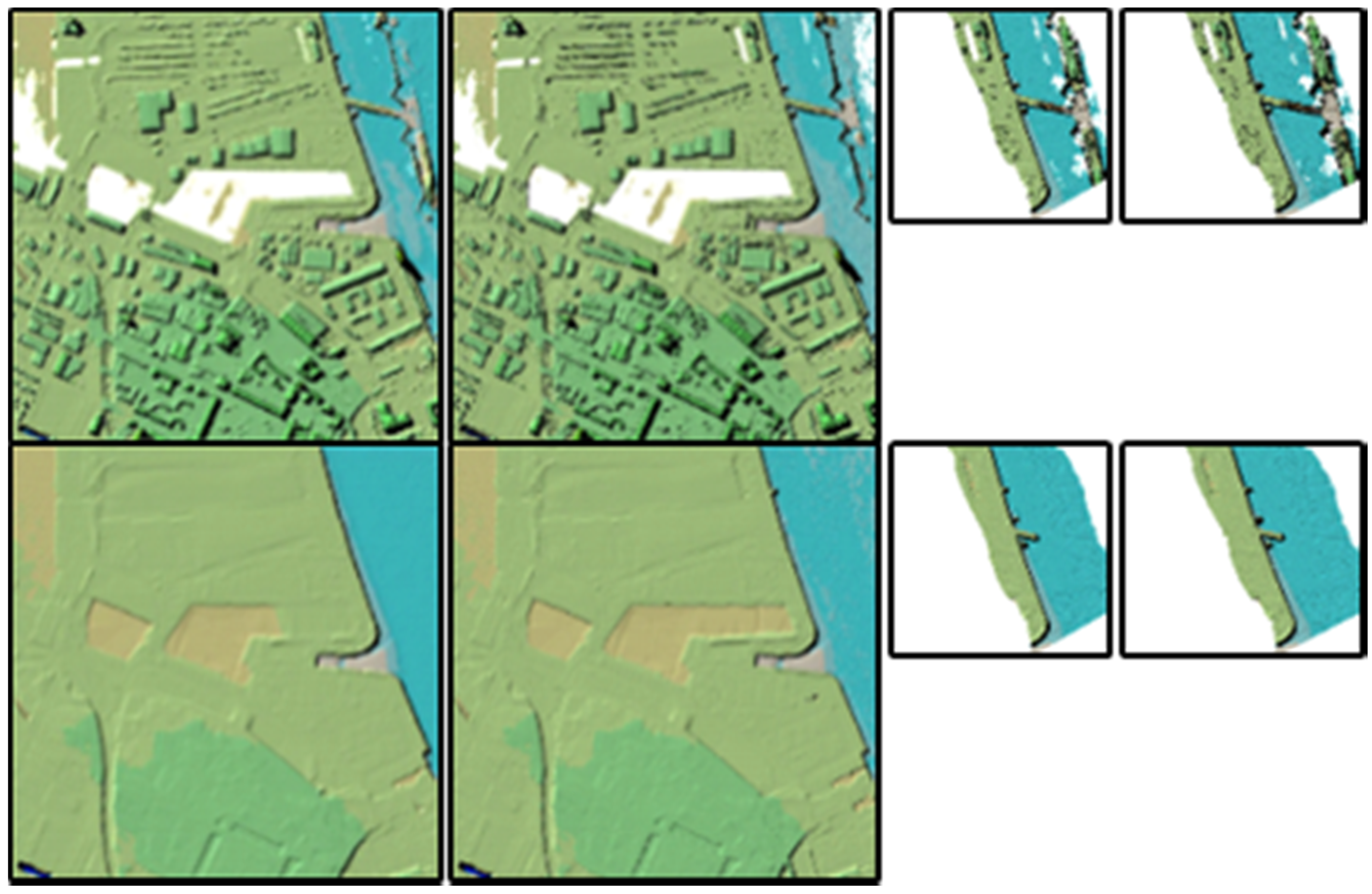
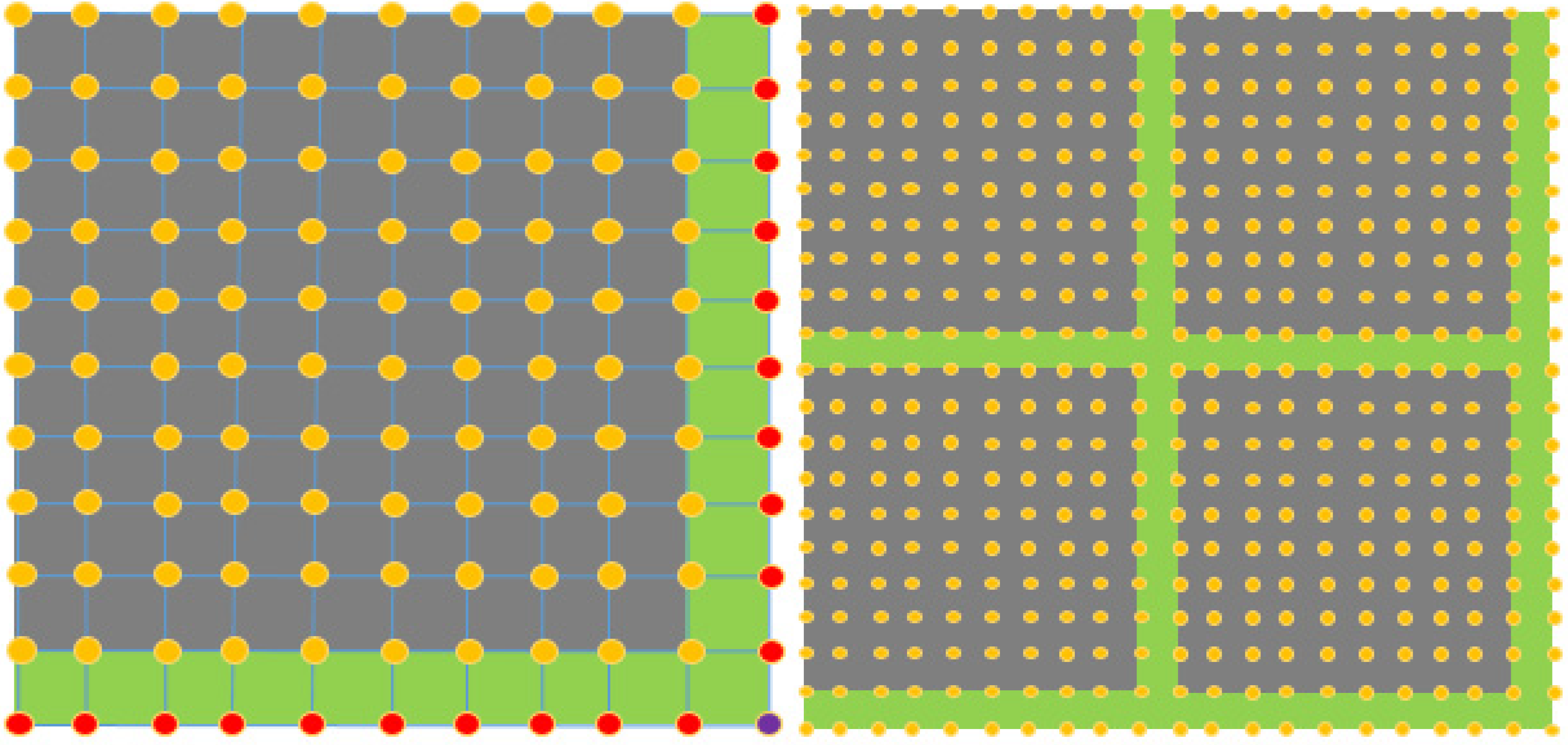
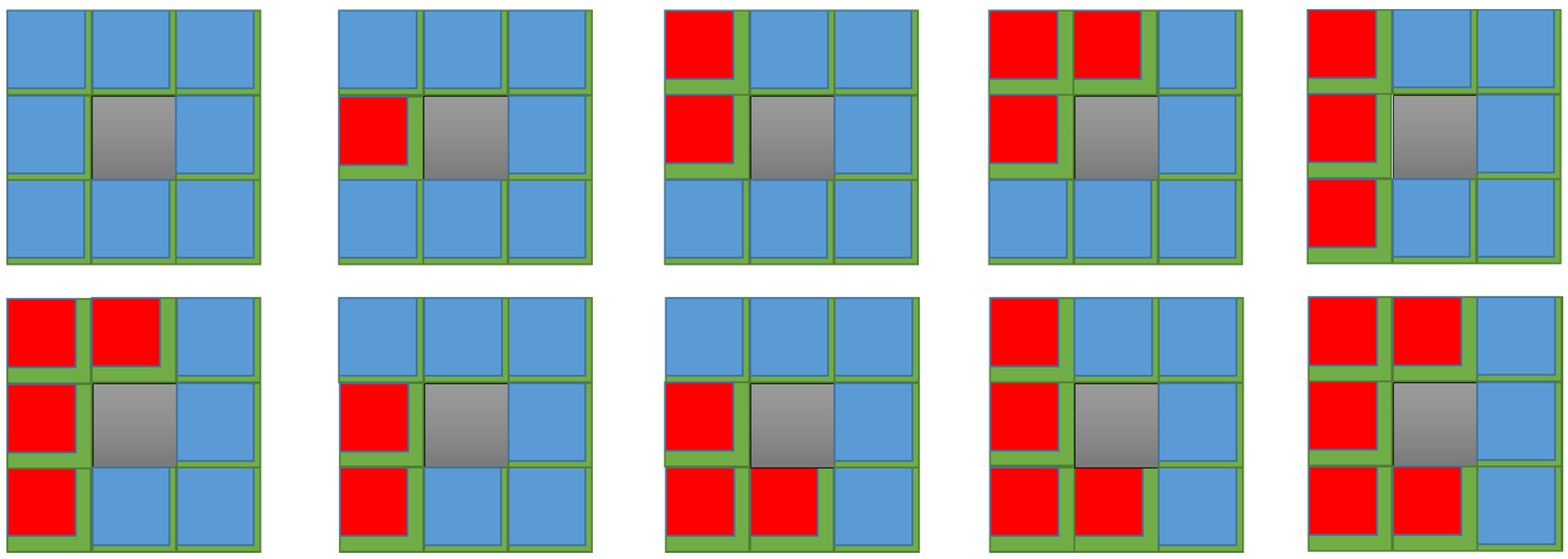
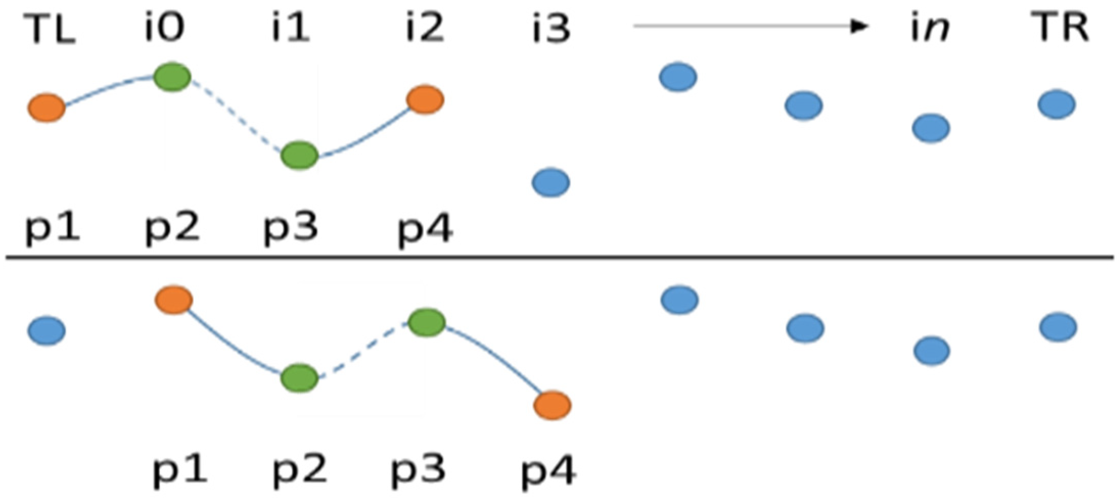
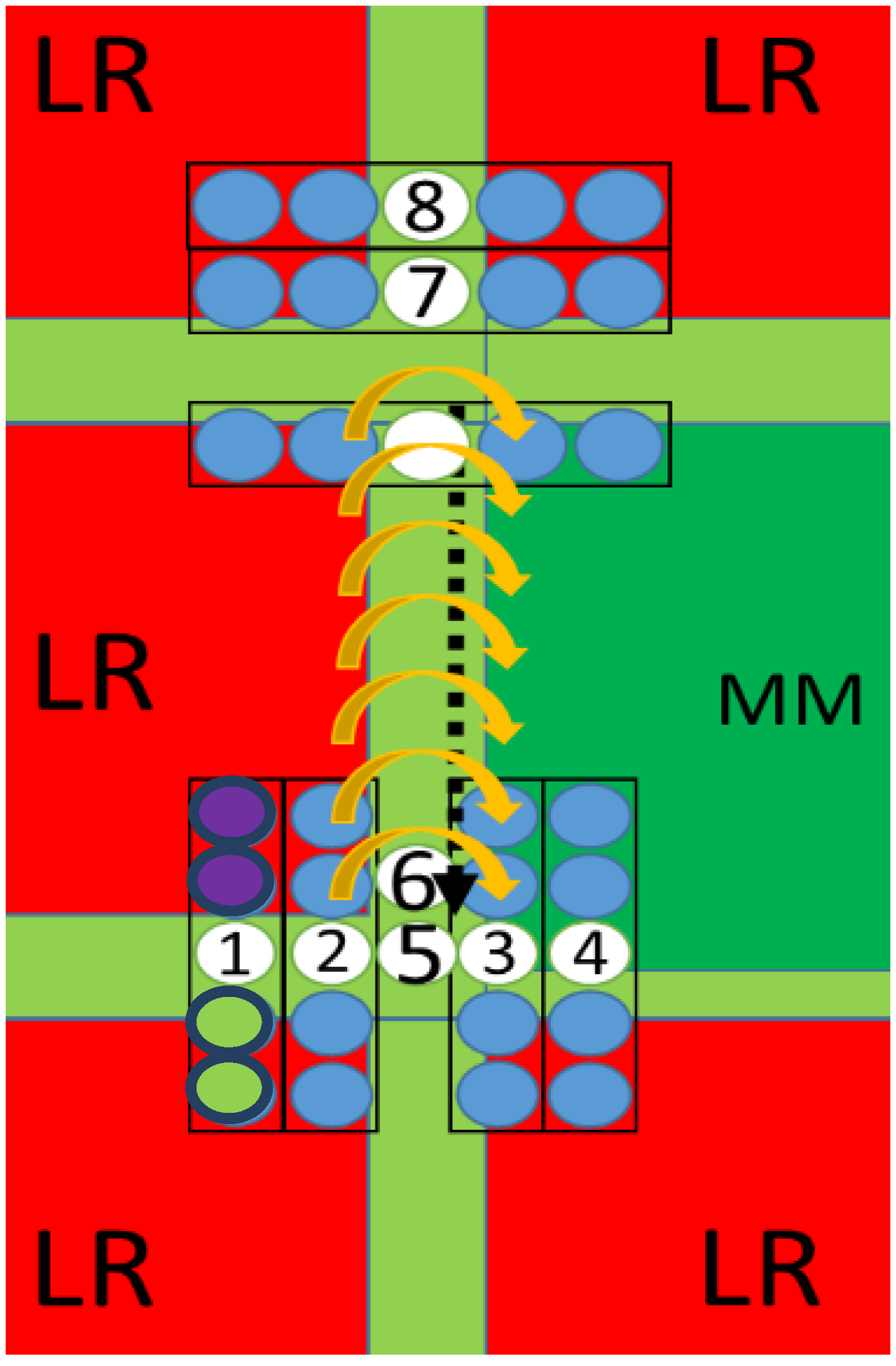
3.2. High Resolution Map Generation

To create high resolution maps, we propose to interpolate missing map data from the lowest resolution, to the highest resolution: OS 50 m to LiDAR 0.25 m using Catmull-Rom interpolation. Catmull-Rom has the benefit of interpolating through control points, and accurate starting tangents by the use of additional control points either side of the interpolation control points. This is important for accurate map generation, especially when interpolating from the 50-m resolution points of OS data to the 2 m LiDAR data due to the large difference in distance between them.

Before we discuss the process of minimising errors by the combination of map data, an issue became apparent at the beginning of the terrain generation process.

However, when generating virtual terrain from map files, the polygons are generated from the outside vertex’s inwards, which is not a problem when only a single map is visualised. When multiple neighbouring maps are needed, a visible skirt of missing polygons appears between neighbouring maps. See Figure 6. A technique proposed by [42] allows smoother LOD transitioning between levels of resolution, and removes the need for stitching meshes. LOD popping is a problem when simulating accurate realism to the user. An alternative to this is to duplicate data from surrounding maps, as represented by the red points and single purple point from Figure 6. This duplication of data can dramatically increase the need for large storage devices, as well as memory at runtime simulation.

With using an optimised binary file format for the generated maps for the complete UK, we estimate a saving of 29.23%, which is equal to 13.22 Terabytes. With added duplicated data, this an extra 16.384 Gigabytes of storage space which is needed. This is only for the highest resolution of 4000² points at 0.25 m cells covering the same coverage of as OS covers and not taking into account other map resolutions. The generation of the binary format file is out of scope for this article.

Figure 6. Skirt of missing data between maps.

Figure 6. Skirt of missing data between maps.

Another issue with the generation of complete maps, maps, which have no missing data but may still contain errors of accuracy, is the differences in the LiDAR data available. Figure 7 shows the differences between the maps. White space represents missing data. Inserting data from the DTM map into the missing data points of the DSM will not generate complete maps due to DTM maps having large areas of missing data. Figure 7 also shows maps generated by combining DSM and DTM data sets.

Figure 7. Hybrid map combination for improved map data.

Figure 7. Hybrid map combination for improved map data.

Process 1 is the combination of DSM and DTM map to exchange data from the DTM to the DSM. If data is still missing, process 2 interpolates lowers resolution map points and combines it with the map from process 1. Process 3 uses map data from OSM to improve height levels by querying OSM boundaries such as water boundaries. Process 4 uses OSM data for the removal of dynamic object heights such as cars on roads. An issue with process 1, working with DTM maps, is the pre-removal of information. The DSM map in process 1 shows a ship and slipway. The DTM map in process 1 has this data removed. The issue is not the removal of the ship but the slipway. This is an issue for creating accurate paths for water vehicles but can be applied to other dynamic artefacts within an urban environment.

Each of these processes has been simulated individually, but has not been combined into a full automated or partial automated programmatic procedure. This is a potential issue with the limit of testing into all possible combinations of maps and OSM data boundaries. Future work will improve this issue.

To generate the missing data, interpolation from lower resolution maps is needed. The Catmull-rom interpolation algorithm uses four points; points 1 and 4 are tangent points used to get the tangent angle entering and leaving points 2 and 3, respectively. It is between points 2 and 3 where interpolation occurs.

To generate missing map data, the left, top, right and bottom tangent interpolation points are needed. The algorithm procedure runs as: combine 2 m DSM and DTM map together, if the map is not complete then generate missing data points from surrounding maps of the same resolution or lower. If a map is lower resolution then multiple interpolation stages are processed.

To generate the left tangent interpolation points, there are a possible 10 combinations of maps, the top interpolation tangent points have five possible combinations, the right interpolation tangent points has five possible combinations, and the bottom interpolation tangent points has 10 possible combinations. The combination consists of the current resolution map we are generating the tangent points at, and the lower resolution map, i.e., the map we want to generate has eight surrounding maps. Conceptually, this can be viewed as a 3 by 3 matrix with the centre index being the map we want generate. To generate the left tangent points, the combination consists of top left map, top map, left map, bottom left map, and the bottom map. Figure 8 shows the combinations needed for the generation of the left tangent points. Red represents lower resolution maps, blue represents the next higher resolution map, and green represents the missing skirt of data between the maps. Notice there are larger skirts on the lower resolution maps.

Figure 8. Map combination for the left tangent points extraction.

Figure 8. Map combination for the left tangent points extraction.

Figure 9 depicts the iterative interpolation technique used to generate values between control points. TL can be thought of as the left tangent point, then being interpolated horizontally through a single row of data from the 2D map to the final right tangent points.

If a neighbour map does not exist then a lower resolution map will be used. If a lower resolution map does not exist, i.e., the map is an edge map of the UK, then tangent interpolation points will be taken from the lower resolution map we are trying to create, i.e., the green map in Figure 10.

Figure 10 shows the procedure needed to generate the left tangent interpolation points for the interpolation of the missing map, depicted as green in Figure 10. As shown, the surrounding maps are all lower resolution. In this case, multiple interpolations using adjacent data points between maps are needed. Points 1, 2, 3, and 4 are needed to create point 5. Each point is generated through interpolation of adjacent points from multiple maps.

Figure 9. Catmull-rom interpolation. “TL” and “TR” represent the tangent points generated from surrounding maps. The “I” represents index position.

Figure 9. Catmull-rom interpolation. “TL” and “TR” represent the tangent points generated from surrounding maps. The “I” represents index position.

Figure 10. Surrounding maps needed for missing map interpolation for higher resolution maps. Left tangent line depicted.

Figure 10. Surrounding maps needed for missing map interpolation for higher resolution maps. Left tangent line depicted.

The first data value loaded from the file is the top left point of the map. This is contradictive to how OS data is explained. OS map naming and referencing are taken from the bottom left, noted as easting and northing, but the OS data within the map can be thought of as upside down, the first value loaded corresponds to the top left point of the map. This is a confusing state of affairs, especially when visualising this data with polygon creation within a game engine to view on screen.

To generate point 1, the lower left map supplies the index (width.max − 1, height.index 1) data point, and index (width.max − 1, height.index 0) data point depicted as green points, and the index (width.max − 1, height.index 0) data point, and index (width.max − 1, height.index − 1) depicted as purple points. Width.max represents the total width of the map, and height.max represents the total height of the map. Width − 1 represents the width value minus 1. Width.index and height.index represent the column and row index respectively. These four points are used as control points and interpolated to create point 1. This process is repeated to create points 2, 3, 4, 7 and 8. Point 5 is generated by points 1, 2, 3, 4 being the control points for interpolation horizontally.

The next process is to interpolate between the left map and the green map horizontally is the same as was done with points 1, 2, 3, and 4, to make point 5, to generate the majority of tangent points. This is depicted by the curve gold arrows and the black dashed arrow line.

With point data generated between the left and centre map, vertical interpolation of the tangent points produces the final array of tangents used in a later process. Point 5 is the tangent point, and point 6 is the control point for the first iteration of the interpolation process. Figure 9 depicts this situation in the top of the image.

Edge and corner maps of the UK are special cases because the tangent points needed cannot be generated due to lack of neighbouring maps. These specific maps are often in the middle of the surrounding oceans of the UK, and need custom procedures. Because of the locations we will not focus map generation techniques for these areas. See Table 3, which shows the number of maps with 1 or more neighbouring maps missing for the 2 m and 1 m LiDAR maps, and also the OS maps after being split into 1 km map segments. The 0.5 m and 0.25 m LiDAR maps cover 500 m², so the left, right, top and bottom missing maps are doubled.

Table 3. Showing the number of maps which do not have certain neighbour maps, for 2 m and 1 m LiDAR maps covering 1 km² and 1 km² subsections of OS maps.

Maps with Missing Neighbours to the:	Count
Left	1300
Right	1300
Top	1100
Bottom	1100
Top-left only	5
Top-right only	4
Bottom-left only	2
Bottom-right only	3
Top Left, Left, Bottom Left, Bottom, Bottom Right	3
Top Right, Right, Bottom Right, Bottom, Bottom Left	4
Bottom Left, Left, Top Left, Top, Top Right	6
Bottom Right, Right, Top Right, Top, Top Left	5

Table 3. Showing the number of maps which do not have certain neighbour maps, for 2 m and 1 m LiDAR maps covering 1 km² and 1 km² subsections of OS maps.

Maps with Missing Neighbours to the:	Count
Left	1300
Right	1300
Top	1100
Bottom	1100
Top-left only	5
Top-right only	4
Bottom-left only	2
Bottom-right only	3
Top Left, Left, Bottom Left, Bottom, Bottom Right	3
Top Right, Right, Bottom Right, Bottom, Bottom Left	4
Bottom Left, Left, Top Left, Top, Top Right	6
Bottom Right, Right, Top Right, Top, Top Left	5

With all surrounding interpolation points generated, interpolation vertically occurs, then horizontally. If a map has data, the interpolation algorithm uses these as control points.

With missing data being created, removing objects from the DSM can be completed by utilising OSM.

The novelty of this paper is the use of OSM building boundary data for the extraction of building meshes from the DSM data. This data can be placed within the DTM data to create a map with reduced dynamic artefacts; cars, flocks of birds, other movable objects etc. OSM also has data locations of trees, bollards, walls and many others, which can be used for the extraction of assets needed for accurate planning. This hybrid combination has the ability to get accurate heights of static artefact: buildings, trees, pylons, which can be used for reduced mesh models for visualisation at runtime.

LiDAR has difficulty penetrating water. OSM brings improvements to LiDAR map generation by the use of water boundaries. Figure 7 shows that combining DSM and DTM maps may remove missing data, but that data may be false positive. Using water boundaries of OSM, these errors in heights can be lowered a specified height value as shown in Figure 7 procedure 3: OSM water boundaries correction. Deciding the height of water levels is complicated due to water ways and rivers may be higher or lower than the sea level state by Ordnance Datum Newlyn.

Within this section we have explained the technique and benefits that a combination of multiple GIS data-sets can bring to hybrid map generation, by reducing errors and removing dynamic objects, while keeping needed data for accurate crisis management planning decisions including for example, planning evacuation routes for crisis events, and proposing emergency developments and resources.

4. Evaluation

In this section we report our experiments to evaluate the performance of our system and techniques to manage complex map data, correct errors and missing data, and identity the best trade-off between maps/terrains resolution and performance. We have used the map densities stated in Table 4 and Table 5 on a desktop computer: Intel Core i7-3770 @ 3.40 GHz, 16.0 GB RAM, 64-bit Operating System, x64-based processor, Windows 8.1 Pro, NVIDIA GeForce GTX 650 Ti graphics card. As stated, the framework is built on top of a game engine. We have used DirectX for this experiment due to the limitless size of vertex buffers. Microsoft.NET does not allow arrays to be over 2 GB, thus, additional configuration files must be added to allow very large objects. We have tested a LiDAR map file covering 1km² containing 1000² height points of Liverpool UK dock lands, producing accurate and realist results running at 751 frames per-second. We have extrapolated and tested the densities directly corresponding to measurements for the testing of maximum potential frame rate to area coverage trade off.

Table 4. Runtime evaluation of visualised terrains at multiple resolutions with single vertex buffers. Only one map is visualised within each scene. The data is captured while the 3D camera is pointing to the centre of the scene, containing all terrain polygons.

Map Dimensions: Points within Map at Meter Cell Size	Index Count	Vertex Count	Polygon Count	FPS	Draw MS	GPU MS	Vertex Buffer Count
5002 points at 2 m 1 km2	1,494,006	250,000	498,002	2,153.98	0.08	0.33	1
10002 points at 1 m 1 km2	5,988,006	1,000,000	1,996,002	751.15	0.18	0.24	1
10002 points at 0.5 m 500 m2	5,988,006	1,000,000	1,996,002	764.99	0.08	1.76	1
20002 points at 0.25 m 500 m2	23,976,006	4,000,000	7,992,002	203.73	0.17	4.56	1
40002 points at 0.25 m 1 km2	95,952,006	16,000,000	31,984,002	51.66	0.23	20.38	1

Table 4. Runtime evaluation of visualised terrains at multiple resolutions with single vertex buffers. Only one map is visualised within each scene. The data is captured while the 3D camera is pointing to the centre of the scene, containing all terrain polygons.

Map Dimensions: Points within Map at Meter Cell Size	Index Count	Vertex Count	Polygon Count	FPS	Draw MS	GPU MS	Vertex Buffer Count
5002 points at 2 m 1 km2	1,494,006	250,000	498,002	2,153.98	0.08	0.33	1
10002 points at 1 m 1 km2	5,988,006	1,000,000	1,996,002	751.15	0.18	0.24	1
10002 points at 0.5 m 500 m2	5,988,006	1,000,000	1,996,002	764.99	0.08	1.76	1
20002 points at 0.25 m 500 m2	23,976,006	4,000,000	7,992,002	203.73	0.17	4.56	1
40002 points at 0.25 m 1 km2	95,952,006	16,000,000	31,984,002	51.66	0.23	20.38	1

Initial test of the 4*4000² representing 2 km² area map at 0.25 m resolution within the framework with, no LOD techniques applied, uses 3.42676 GB of memory.

Figure 11 and Table 4 shows the relation between FPS and polygon count for a map. We observe that the FPS to polygon count correlation between map sizes of 10002 points at 1 m 1 km² and 10,002 points at 0.5 m 500 m² are different by 13.84, even though they are the same size in index count, vertex count, and polygon count. This could be because of culling techniques used by the graphics card. Further research is needed to account for this issue.

We can see that the technique for generating large and complex maps has a good performance and is able to process with an acceptable frame rate and rendering time, up to 16 million polygons for a map dimension of 4000² at 0.25 m.

Figure 11. Graph showing the correlation between frames per second and polygon count of single vertex buffers.

Figure 11. Graph showing the correlation between frames per second and polygon count of single vertex buffers.

Table 5. Runtime evaluation of visualised terrains at multiple resolutions with multiple vertex buffers.

Map Dimensions: Points within Map at Meter Cell Size	Index Count	Vertex Count	Polygon Count	FPS	Draw MS	GPU MS	Vertex Buffer Count
1*20002 points at 0.25 m 500 m2	23,976,006	4,000,000	7,992,002	203.73	0.17	4.56	1
2*20002 points at 0.25 m 500 m2	47,952,012	8,000,000	15,984,004	103.41	0.18	9.52	2
4*20002 points at 0.25 m 500 m2	95,904,024	16,000,000	31,968,008	52.04	0.19	18.76	4
8*20002 points at 0.25 m 500 m2	191,808,048	32,000,000	63,936,016	11.75	0.26	84.64	8
1*40002 points at 0.25 m 1 km2	95,952,006	16,000,000	31,984,002	51.66	0.17	18.51	1
2*40002 points at 0.25 m 1 km2	191,904,012	32,000,000	63,968,004	12.81	0.26	71.92	2
4*40002 points at 0.25 m 1 km2	383,808,024	64,000,000	127,936,008	4.68	0.27	211.99	4
8*40002 points at 0.25 m 1 km2	767,616,048	128,000,000	255,872,016	X	XX	X	8

Table 5. Runtime evaluation of visualised terrains at multiple resolutions with multiple vertex buffers.

Map Dimensions: Points within Map at Meter Cell Size	Index Count	Vertex Count	Polygon Count	FPS	Draw MS	GPU MS	Vertex Buffer Count
1*20002 points at 0.25 m 500 m2	23,976,006	4,000,000	7,992,002	203.73	0.17	4.56	1
2*20002 points at 0.25 m 500 m2	47,952,012	8,000,000	15,984,004	103.41	0.18	9.52	2
4*20002 points at 0.25 m 500 m2	95,904,024	16,000,000	31,968,008	52.04	0.19	18.76	4
8*20002 points at 0.25 m 500 m2	191,808,048	32,000,000	63,936,016	11.75	0.26	84.64	8
1*40002 points at 0.25 m 1 km2	95,952,006	16,000,000	31,984,002	51.66	0.17	18.51	1
2*40002 points at 0.25 m 1 km2	191,904,012	32,000,000	63,968,004	12.81	0.26	71.92	2
4*40002 points at 0.25 m 1 km2	383,808,024	64,000,000	127,936,008	4.68	0.27	211.99	4
8*40002 points at 0.25 m 1 km2	767,616,048	128,000,000	255,872,016	X	XX	X	8

The experiments results look promising in regards to visualizing highly dense polygon scenes at real-time frame rates. Further analysis has to be carried out into the best situation for the splitting of maps. The splitting of a 4000² map at 0.25 m resolution to a 4 neighbouring 2000² maps at 0.25 m resolution contains 4 vertex buffers to cover 1 km², which increases the frame rate by 0.33 fps. The GPU draw time is reduced from 0.23 ms, to 0.19 ms. A question is raised whether the speed increase is due to bus-speed transfer from CPU to GPU, or is it the reduction of polygons the GPU has to rasterise. The splitting of a map adds the issues of missing skirt information as stated earlier, removing 47,982 polygons from the scene. Table 5 shows multiple maps generated at 0.25 m resolution covering 500 m² and 1 km². As you can see from the last row in Table 5, the 8*40,002 points at 0.25 m 1 km² visualisation frame rate is below a frame a second and we were unable to gather measurements. We can compare the fps of our implementation to the work of [43]. They generated a LiDAR ground surface model (DGM) consisting of 1,659,958 vertices with 3,228,653 polygons at 6.3 fps on a Intel-XeonX5650 @ 2.67 Ghz(x6).

NVIDIA-Quadro5000 system. The system they use is often used as a specialized workstation using CAD software, as opposed to our off the shelf configuration with a more modern advanced GPU.

5. Conclusion

In this paper we have discussed the use of Games Technologies for the research and development of 3D virtual environments representing real environments captured from GIS information and Open source map data. The challenges involved in these research areas concern the large amount of data to be dealt with, as well as some map data, which include errors and are not complete. The domain of application of our work is crisis management, which requires very accurate GIS or map information, as well as data that is manageable and user friendly. We have proposed and tested procedures for improved map generation techniques combining real-world maps using LiDAR, OSM, and OS data for terrain generation. We have also stated improvements in storage space by saving maps in an optimised file format. Evaluations of initial tests stress testing a C# game engines rendering capabilities and concluded that with additional advanced rendering techniques, large, highly dense, and accurate map visualisations over multiple kilometres is achievable at a comfortable frame-rate.

The differentiation of multiple GIS data sets and programming of map processors has been more complex than first thought. To complete our framework, we must complete future work. The generation algorithm for hybrid map generation needs to be tested and completed to allow additional data to be combined, as well as increased OSM integration. For example, using the road system of OSM to smooth out dynamic objects on the LiDAR maps where roads will be placed.

LOD techniques need to be added to the framework to allow larger terrain coverage. Once larger terrains are visible on screen, and map data is complete, i.e., contains no missing data but can still be error prone, then automated planning algorithms can be tested within the framework while viewing the results in real-time.

6. Future Work

Our future work consists of completing and programming a semi-automatic procedure, which can combine the multiple map data sets into a hybrid layered representation capable of querying a user to supersede its own decisions.

Research and testing of multiple interpolation techniques are needed to decide which techniques are a more accurate representation when interpolating from a lower resolution to a higher resolution dataset. We intend to test: linear, cubic, sinusoidal, exponential, quadratic, and quantic interpolation functions. The classification and testing of these interpolation functions are needed for the large criteria of data sets we have worked with in this paper.

The creation 3D virtual environments using real world map data whilst correcting and completing missing data will improve quality and performance of a crisis management decision support system and provide a more natural and intuitive interface for crisis managers. Usability testing will need to be expanded and tested which requires further research into the currently implemented crisis management decision support systems. To increase usability and interface analysis, discussions with real-world crisis managers are needed to discuss and criticize the applicability of initial ideas.

Improved error reduction techniques are needed to minimize error within the underlining data sets. Using a 3D application providing by a game engine, a user can view scenes and if large errors are within a virtualized scene, such as flocks of birds inflight, introducing large errors in the LiDAR DSM data-sets, the user can query this error and remove it from the data-set. This is a large task to accomplish, so to speed the procedure, procedural error checking can be implemented to query building bounding data from the OSM data-sets, if a large spike of error is within this boundary, but the OSM data-set states that the building of only of a certain height, the issue can be logged for further inspection by a user.

The need to implement flooding visualisation techniques other than using a single plane representing water level is needed to combine the enriched hybrid maps to monitor flood pooling to create future artificial intelligent path finding world representations custom for individual agents.

For improved visualization of scenes, the need for advanced techniques for the rendering of objects within a scene are needed, such as: real-time water, night and day simulations, improved road systems for curved roads, improved procedural generation of procedural buildings, added physics engine, simplified weather simulation depicting rain, LOD techniques, and advanced shader techniques for highlighting potential errors or hotspots in scenes.

References

1. Folger, P. Geospatial Information and Geographic Information Systems (GIS): Current Issues and Future Challenges; DIANE Publishing: Collingdale, PA, USA, 2009. [Google Scholar]
2. What is GIS. Available online: http://www.esri.com/what-is-gis (accessed on 30 March 2015).
3. Folger, P. Geospatial Information and Geographic Information Systems (GIS ): An Overview for Congress; DIANE Publishing: Collingdale, PA, USA, 2011. [Google Scholar]
4. Miller, A. Trends in process control systems security. IEEE Secur. Priv. 2005, 3, 57–60. [Google Scholar] [CrossRef]
5. Robertson, G.; Mary, C.; Van Dantzich, M. Immersion in desktop virtual reality. In Proceedings of the 10th Annual ACM Symposium on User Interface Software and Technology, Banff, AB, Canada, 14–17 October 1997.
6. Mihail, R.P.; Goldsmith, J.; Jacobs, N.; Jaromczyk, J.W. Teaching graphics for games using Microsoft XNA. In Proceedings of 18th International Conference on Computer Games: AI, Animation, Mobile, Interactive Multimedia, Educational & Serious Games, Louisville, KY, USA, 30 July–1 August 2013.
7. Bourke, P. Low cost projection environment for immersive gaming. J. Multimed. 2008, 3, 41–46. [Google Scholar] [CrossRef]
8. Geomatics Group: Aerial LIDAR Data, Aerial Photography and Spatial Data. Available online: https://www.geomatics-group.co.uk/geocms/ (accessed on 30 March 2015).
9. Cheng, L.; Gong, J.; Li, M.; Liu, Y. 3D building model reconstruction from multi-view aerial imagery and lidar data. Photogramm. Eng. Remote Sens. 2011, 77, 125–139. [Google Scholar] [CrossRef]
10. Leberl, F.; Irschara, A.; Pock, T.; Meixner, P.; Gruber, M.; Scholz, S.; Wiechert, A. Point Clouds: Lidar versus 3D Vision. Photogramm. Eng. Remote Sens. 2010, 76, 1123–1134. [Google Scholar] [CrossRef]
11. OpenStreetMap.Org. Available online: http://www.openstreetmap.org/#map=15/53.4312/-2.8737 (accessed on 23 June 2015).
12. Britain’s Mapping Agency | Ordnance Survey. Available online: http://www.ordnancesurvey.co.uk/ (accessed on 30 March 2015).
13. Parish, Y.I.H.; Müller, P. Procedural modeling of cities. In Proceedings of the 28th Annual Conference on Computer Graphics and Interactive Techniques, Los Angeles, CA, USA, 12–17 August 2001.
14. Bradley, B. Towards the Procedural Generation of Urban Building Interiors Table of Contents. Master’s Thesis, University of Hull, Yorkshire, UK, 2005. [Google Scholar]
15. Wonka, P.; Aliaga, D.; Müller, P.; Vanegas, C. Modeling 3D urban spaces using procedural and simulation-based techniques. In Proceedings of the 2011 Annual Conference on Computer Graphics and Interactive Techniques, Hong Kong, China, 7–11 August 2011.
16. Yannakakis, G.N.; Togelius, J. Experience-driven procedural content generation. IEEE Trans. Affect. Comput. 2011, 2, 147–161. [Google Scholar] [CrossRef]
17. Chaplot, V.; Darboux, F.; Bourennane, H.; Leguédois, S.; Silvera, N.; Phachomphon, K. Accuracy of interpolation techniques for the derivation of digital elevation models in relation to landform types and data density. Geomorphology 2006, 77, 126–141. [Google Scholar] [CrossRef]
18. Twigg, C. Catmull-rom splines. Computer 2003, 41, 4–6. [Google Scholar]
19. Marschner, S.R.; Lobb, R.J. An evaluation of reconstruction filters for volume rendering. In Proceedings of 1994 IEEE Visualization Conference, Washington, DC, USA, 17–21 October 1994.
20. Dudenhoeffer, D.; Hartley, S.; Permann, M. Critical infrastructure interdependency modeling: A survey of critical infrastructure interdependency modeling. Available online: http://www5vip.inl.gov/technicalpublications/Documents/3489532.pdf (accessed on 23 June 2015).
21. Hernantes, J.; Rich, E.; Laugé, A.; Labaka, L.; Sarriegi, J.M. Learning before the storm: Modeling multiple stakeholder activities in support of crisis management, a practical case. Technol. Forecast. Soc. Change 2013, 80, 1742–1755. [Google Scholar] [CrossRef]
22. Aqil, M.; Kita, I.; Yano, A.; Soichi, N. Decision support system for flood crisis management using artificial neural network. Int. J. Intell. Technol. 2006, 1, 70–76. [Google Scholar]
23. Rinaldi, S. Modeling and simulating critical infrastructures and their interdependencies. In Proceedings of the 37th Annual Hawaii International Conference on System Sciences, Big Island, HI, USA, 5–8 January 2004.
24. Kwan, M.P.; Lee, J. Emergency response after 9/11: The potential of real-time 3D GIS for quick emergency response in micro-spatial environments. Comput. Environ. Urban Syst. 2005, 29, 93–113. [Google Scholar] [CrossRef]
25. Smelik, R.; Tutenel, T. Interactive creation of virtual worlds using procedural sketching. In Proceedings of the 2010 Eurographics, Norrköping, Sweden, 4–7 May 2010.
26. Cui, X.; Shi, H. A*-based pathfinding in modern computer games. Int. J. Comput. Sci. Netw. Secur. 2011, 11, 125–130. [Google Scholar]
27. Kumar, P.; Bottaci, L.; Mehdi, Q.; Gough, N.; Natkin, S. Efficient path finding for 2D games. In Proceedings of the 5th International Conference on Computer Games: Artificial Intelligence, Design and Education, Leicester, UK, 8–10 November 2004.
28. Björnsson, Y.; Halldórsson, K. Improved heuristics for optimal path-finding on game maps. In Proceedings of the Second Artificial Intelligence and Interactive Digital Entertainment Conference, Marina del Rey, CA, USA, 20–23 June 2006.
29. Graham, R.; McCabe, H.; Sheridan, S. Pathfinding in computer games. ITB J. 2003, 8, 57–81. [Google Scholar]
30. Kumari, S.; Geethanjali, N. A survey on shortest path routing algorithms for public transport travel. Glob. J. Comput. Sci. 2010, 9, 73–76. [Google Scholar]
31. Smith, G.; Whitehead, J.; Mateas, M. Tanagra: Reactive planning and constraint solving for mixed-initiative level design. Comput. Intell. AI Games 2011, 3, 201–215. [Google Scholar]
32. Isaacs, J.P.; Falconer, R.E.; Gilmour, D.J.; Blackwood, D.J. Enhancing urban sustainability using 3D visualisation. Available online: https://repository.abertay.ac.uk/jspui/bitstream/10373/1122/1/udap164-163.pdf (accessed on 23 June 2015).
33. Kellomäki, T. Interaction with dynamic large bodies in efficient, real-time water simulation. J. WSCG 2013, 21, 117–126. [Google Scholar]
34. Piccoli, C. CityEngine for Archaeology. Available online: http://www.academia.edu/10586805/CityEngine_for_Archaeology (accessed on 23 June 2015).
35. CyberCity3D. Available online: http://www.cybercity3d.com/newcc3d/ (accessed on 27 May 2015).
36. Togelius, J.; Friberger, M.G. Bar Chart Ball, a Data Game. In Proceedings of the 8th International Conference on the Foundations of Digital Games, Crete, Greece, 24 June 2013.
37. Friberger, M.G.; Togelius, J.; Cardona, A.B.; Ermacora, M.; Mousten, A.; Jensen, M.M. Data games. In Proceedings of 2013 Foundations of Digital Games, Crete, Greece, 14–17 May 2013.
38. Tully, D.; El Rhalibi, A.; Merabti, M.; Shen, Y.; Carter, C. Game based decision support system and visualisation for crisis management and response. In Proceedings of the 15th Annual PostGraduate Symposium on the Convergence of Telecommunications, Networking and Broadcasting, Liverpool, UK, 24 June 2014.
39. MonoGame | Write Once, Play Everywhere. Available online: http://www.monogame.net/ (accessed on 30 March 2015).
40. Indraprastha, A.; Shinozaki, M.; Program, U.D. The investigation on using Unity3D game engine in urban design study. J. ICT Res. Appl. 2009, 3, 1–18. [Google Scholar] [CrossRef]
41. Jokinen, P.; Tarhio, J.; Ukkonen, E. A comparison of approximate string matching algorithms. Software—Practice Exp. 1996, 26, 1–4. [Google Scholar] [CrossRef]
42. Strugar, F. Continuous distance-dependent level of detail for rendering heightmaps. J. Graph. GPU Game Tools. 2009, 14, 1–15. [Google Scholar] [CrossRef]
43. Manya, N.; Ayyala, I.; Benger, W. Cartographic rendering of elevation surfaces using procedural contour lines. In Proceedings of 21st WSCG International Conferences in Central Europe on Computer Graphics, Visualization and Computer Vision, Prague, Czech Republic, 20 May 2013.