Multidimensional Spatial Vitality Automated Monitoring Method for Public Open Spaces Based on Computer Vision Technology: Case Study of Nanjing’s Daxing Palace Square

Abstract

Assessing the vitality of public open spaces is critical in urban planning and provides insights for optimizing residents’ lives. However, prior research has fragmented study scopes and lacks fine-grained behavioral data segmentation capabilities and diverse vitality dimension assessments. We utilized computer vision technology to collect fine-grained behavioral data and proposed an automated spatial vitality monitoring framework based on discrete trajectory feature points. The framework supported the transformation of trajectory data into four multidimensional vitality indicators: crowd heat, resident behavior ratio, movement speed, and spatial participation. Subsequently, we designed manual validation mechanisms to demonstrate the monitoring framework’s efficacy and utilized the results to explore the changes in vitality, and the influencing factors, in a small public space. Discrete trajectory feature points effectively addressed the literature’s fragmented study scope and limited sample size issues. Spatial boundaries had a significantly positive impact on spatial vitality, confirming the “boundary effect” theory. The peak spatial vitality periods were from 08:30 to 09:30 and from 17:30 to 18:30. A higher enclosure degree and better rest facilities positively impacted spatial vitality, while a lower enclosure degree did not consistently suppress spatial vitality in all situations. Overall, spatial features and spatial vitality have a complex nonlinear relationship.

1. Introduction

Public open spaces are essential elements of urban life and are significant for public health, safety, and quality of life [1,2,3,4]. In recent years, China has embarked on extensive public open space renovation projects to address the urban challenges arising from rapid urbanization [5,6]. Humanistic and precise planning and transformation have become mainstream approaches, supplanting “the grand narrative” concept in urban spatial planning and construction [7]. This necessitates researchers to macroscopically monitor urban accessibility and the physical environment while microscopically re-evaluating public open spaces from the humancentric perspective [8,9,10,11,12,13]. Based on Jacobs’ humanistic urban studies [14], numerous researchers have emphasized the importance of crowd behavior to assess spatial vitality in public open spaces. Specifically, they have argued that crowd behavior can mirror spatial vibrancy and utilization, offering a foundation for urban designers to enhance public open-space environments and elevate residents’ well-being [15,16,17]. However, the acquisition of detailed crowd behavior data and the establishment of an equivalent relationship between crowd behavior information and spatial vitality continue to pose challenges in public open space research [18,19]. For example, emerging technologies that rely on big data, global positioning system (GPS) location data [20,21,22], mobile signaling [2,18,23], social media data [24,25], and multisource big data have effectively assisted researchers in improving the efficiency of urban crowd behavior data acquisition [15,26,27,28]. However, in contrast to macroscale urban spatial vitality research, which prioritizes data breadth, microscale studies have exhibited heightened sensitivity toward the granularity of behavioral information, geographical positioning accuracy, and temporal coherence [29]. Moreover, owing to data granularity and collection limitations, large-scale behavioral datasets are insufficient for application at the microscale [30]. Therefore, researchers must identify a suitable method for acquiring small-scale spatial behavioral data that offers a convenient and efficient data acquisition approach while meeting the precision requirements of empirical research.

To obtain fine-grained behavioral data, mainstream behavioral data collection modes include questionnaire surveys and behavioral annotation methods [31,32,33,34], which are low-throughput approaches. Meanwhile, traditional manual statistics are inefficient, lack generalizability, and exhibit strong subjectivity when annotating the locations of behavioral data, making it difficult to record dynamic changes in activity over time. Wi-Fi probe technology has emerged as a method for acquiring small-scale spatial behavioral data, with significant advantages in terms of coverage and efficiency [35]. However, data interference caused by environmental obstructions and non-mobile-phone crowds cannot be avoided. In comparison, video data can faithfully represent human activities, provide rich and precise behavioral trajectory information, and include body movements and facial expressions, thus offering multidimensional raw data for behavioral research. Therefore, building on Whyte’s early work [36], some researchers have combined video data with emerging computer vision (CV) to develop video computer recognition technology that can quantitatively capture crowd behavior information. The effectiveness of video computer recognition technology has been verified via social behavior monitoring [37], public open space pedestrian flow distribution [38], and walking behavior assessments [39]. Moreover, with the simultaneous support of fine-grained data, the relationship between crowd behavior and the physical environment of public open spaces has been analyzed at the microscale. For example, Loo et al. [40] constructed a regression model between social activities and interactive landscape features to analyze the relationship between urban furniture and social activities. Wei et al. [41] sampled surveillance videos from 16 urban streets to establish the relationship between behavioral preferences and urban physical boundaries. Furthermore, some studies have linked crowd behavior characteristics to spatial vitality, explored new factors representing spatial vitality [42], and constructed spatial vitality proxy models for automated spatial vitality assessment [29]. While these studies have indicated that using video computer recognition technology is a reliable approach for acquiring behavioral data since it combines the data granularity advantages of traditional manual statistics with the data collection efficiency and objectivity of emerging technologies, there are unresolved issues in public open space vitality research based on crowd behavior. First, most studies have been confined to evaluations within the boundaries of independent video frames [29,40]; as such, they have failed to link data samples from multiple viewpoints and have prevented a holistic analysis of the spatial vitality distribution in a public open space. Second, some studies have used complete behavioral trajectories as statistical units [29], or relied solely on grid-based methods to count pedestrian movements [38], hindering spatiotemporal behavioral feature segmentation. Finally, most studies have considered a single population quantity metric to represent spatial vitality [38,41]; as such, they have failed to provide a multidimensional exploration of crowd behavior characteristics.

Accordingly, we propose a method for measuring crowd behavior characteristics using discrete weighted trajectory feature points as statistical units. Consequently, human behavioral characteristics can be expressed within a single trajectory feature point. Furthermore, by using weighted calculations to associate neighboring trajectory feature points and retain continuous trajectory features, we provide an effective solution for integrating data from multiple viewpoints [17], thereby addressing the challenges of spatiotemporal behavioral feature segmentation. Finally, we analyze the distribution of spatial vitality among different spatial features of a public open space. Our main research questions are as follows:

How can we build an automated monitoring model using detailed population behavior data to characterize spatial vitality?

Are there spatial distribution differences in spatial vitality during different periods?

Do spatial vitality characteristics vary heterogeneously for different spatial features?

2. Methods

2.1. Methodology Framework Overview

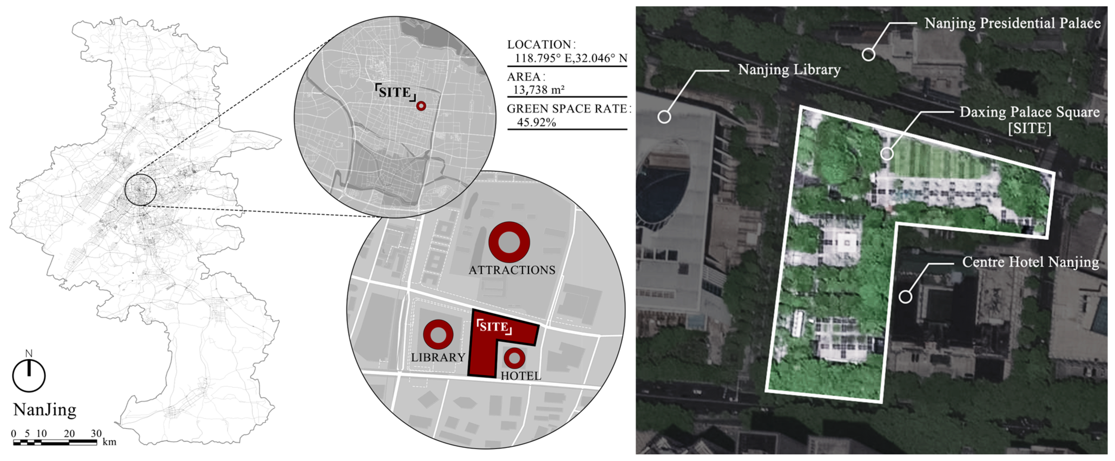
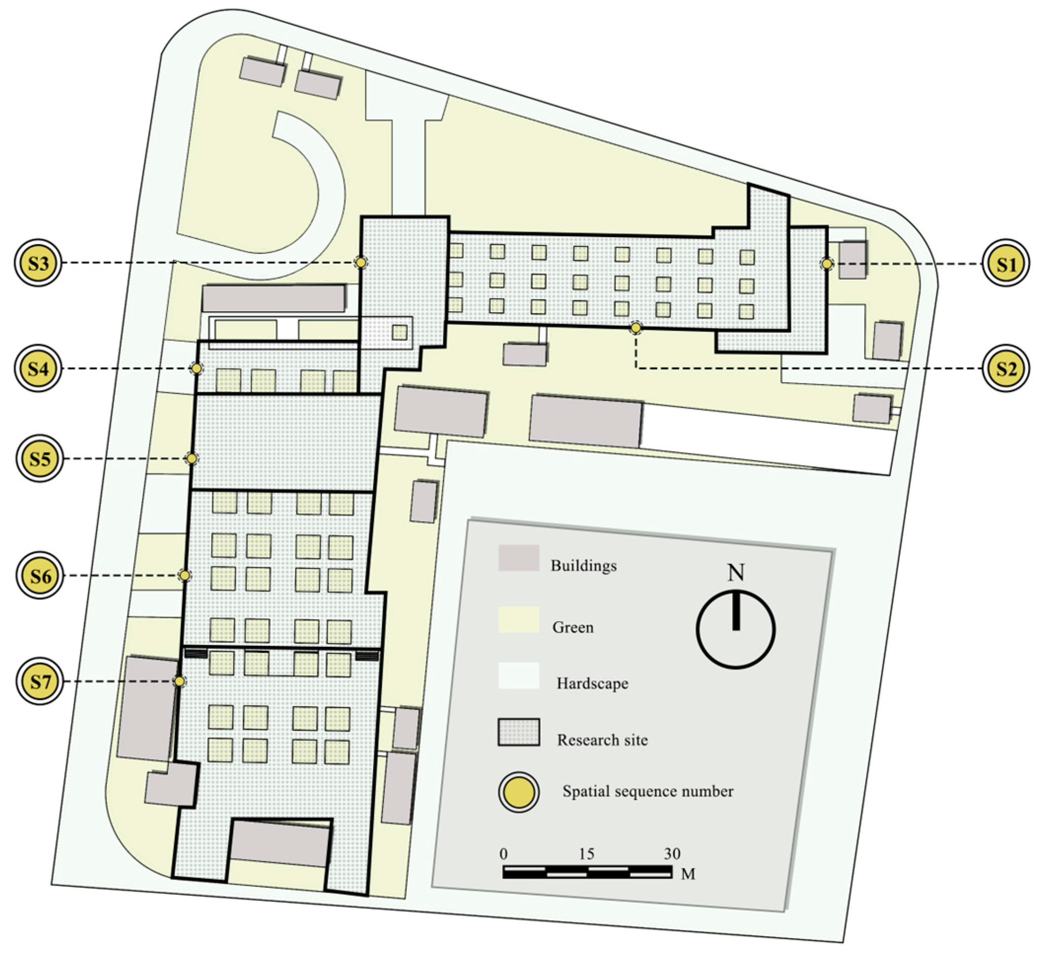
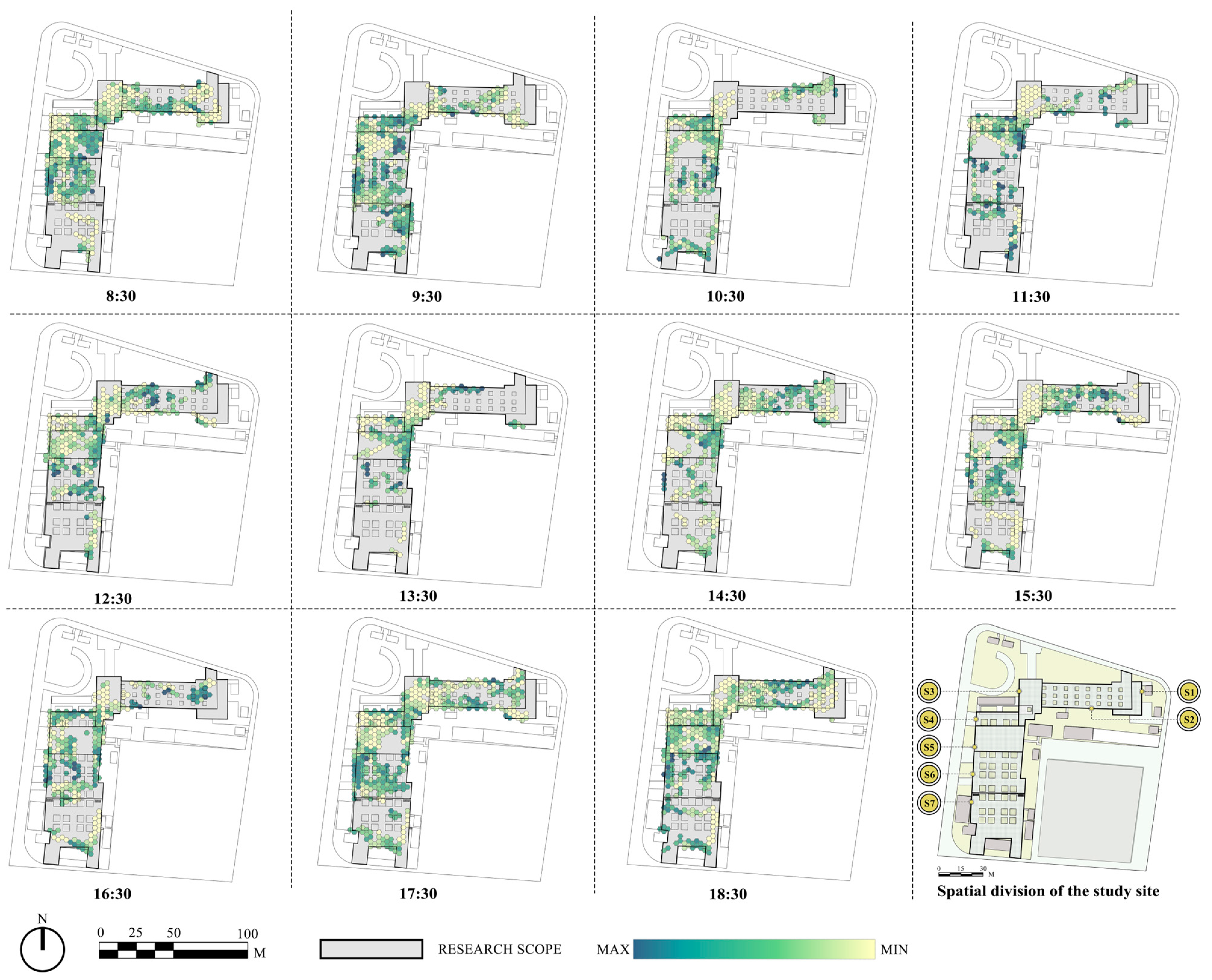
We first collected video datasets capable of replicating crowd behavior within the study site, which we then partitioned into seven internally homogeneous independent spatial units. Subsequently, we used a computerized automated monitoring framework to quantify the multidimensional spatial vitality of the research site. Specifically, we deployed the YOLOv7-DeepSort model on the Python platform to extract pedestrian trajectories from videos. We then developed a method for quantifying spatial vitality from four dimensions: crowd heat, staying behavior ratio, movement speed, and spatial participation. For detailed methodologies, see Section 2.3 and Section 2.4. Then, we designed a set of manual assessment and verification methods, with each metric corresponding to the automated monitoring results. Finally, we divided the study site into hexagonal grids. Each hexagonal grid area corresponded to the staying behavior recognition threshold. We selected hexagonal grid shapes because of their strong statistical properties for trajectory data [40]. We linked the trajectory feature point data to a grid to ascertain the average feature index of each spatial unit, facilitating the construction of spatial distribution maps. This approach enabled our investigation of the distribution of and variation in spatial vitality factors for different spatial features in the spatiotemporal dimensions. Figure 1 shows the research process.

2.2. Study Site

In the preliminary design phase of our study, we first established criteria for selecting the research site. Firstly, due to the need for repeated experiments in method exploration, the research site should be of appropriate size and free of excessive obstructions. This ensures that utilizing multiple camera positions to cover the research area will not incur excessively high research costs. Secondly, the site should have a high level of activity richness to validate the stability of the space vitality monitoring method in analyzing different trajectory characteristics. Thirdly, the site should have multiple spaces with distinct spatial features, aiding in testing the stability of the space vitality monitoring method under various spatial characteristics and exploring the differences in space vitality across different spatial features.

Ultimately, our research site was chosen to be Daxing Palace Square, Nanjing, southeast China (118°22′ E–119°14′ E, 31°14′ N–32°37′ N). Daxing Palace Square covers an area of 13,738 m² and is free of excessive obstructions. It is located in the densely populated Xuanwu District, adjacent to the city’s significant attractions, such as Nanjing Presidential Palace, and a municipal library (Figure 2). This location has high pedestrian flow and a rich variety of activities. Additionally, the square contains diverse small space types, including fully covered and semi-covered tree-lined squares and open hard-surfaced squares of varying sizes. Therefore, Daxing Palace Square meets our research requirements and was selected as our research site.

2.3. Obtaining the Research Data

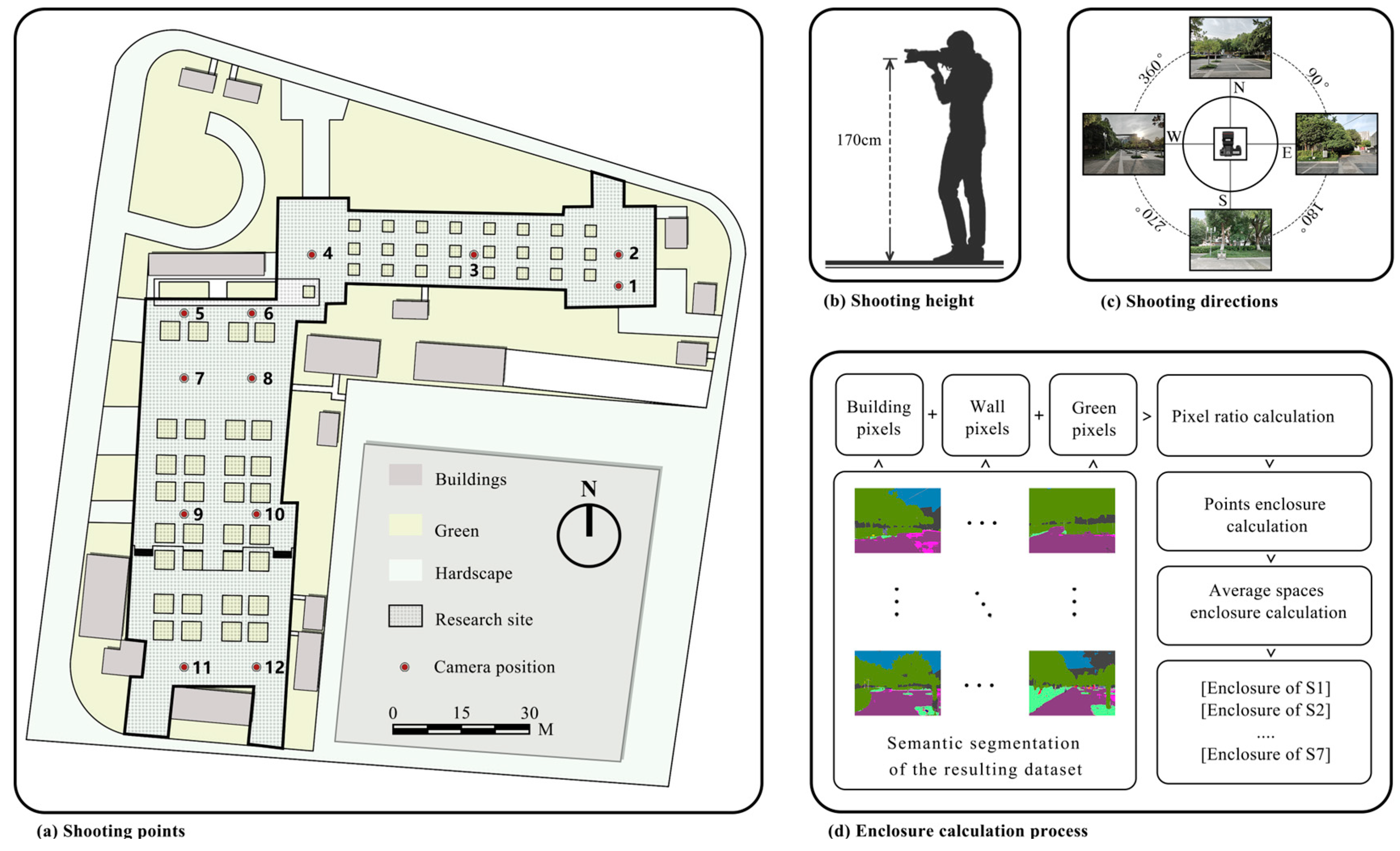
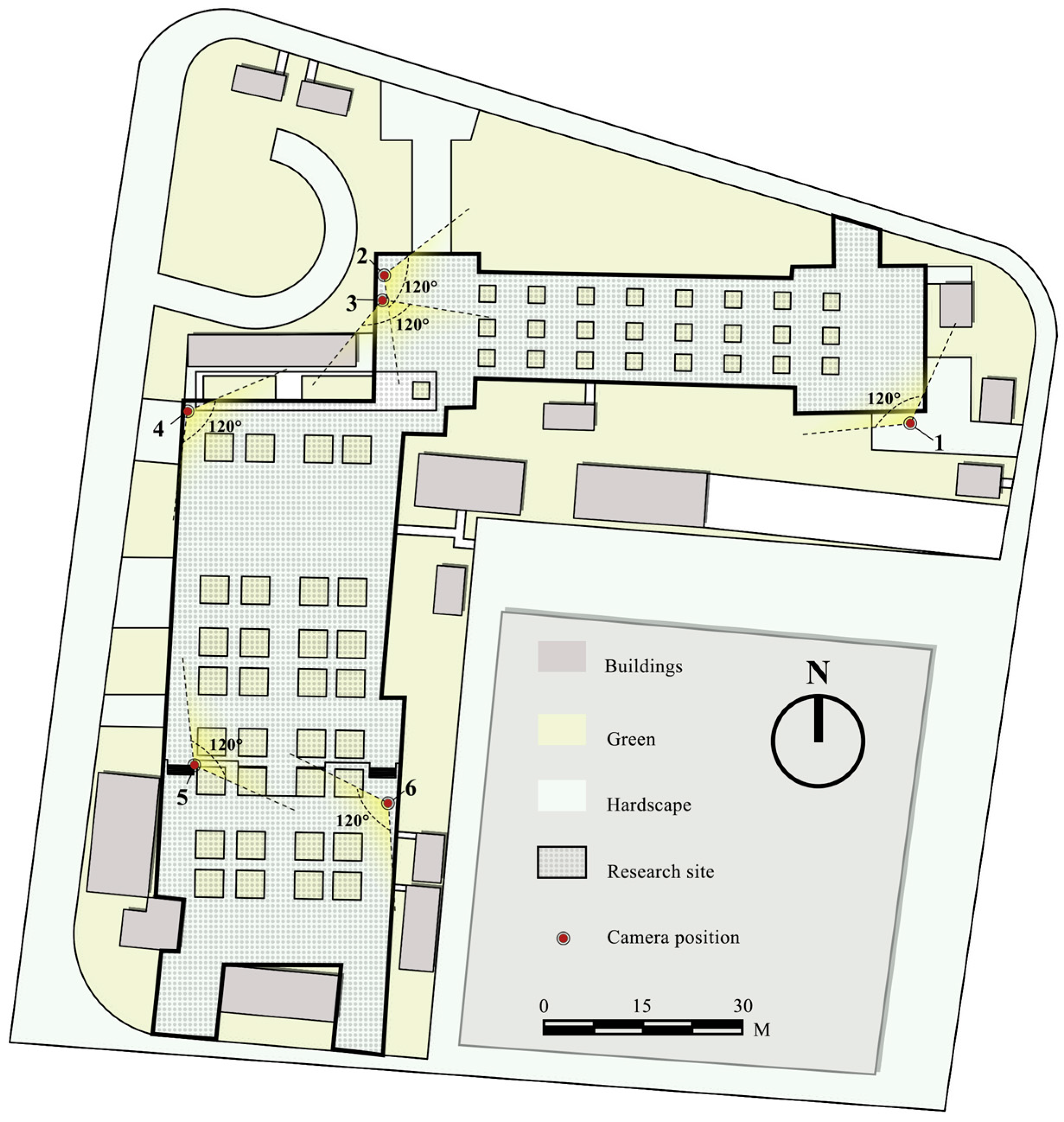
2.3.1. Quantification of Physical Site Environment

During our spatial vitality assessments and analyses of the study site, averaging the overall vitality level of the site may have led to the mutual interference of pedestrian data for different spatial features, reduced data granularity, and resulted in biased analyses. Therefore, our study site required further subdivision, based on its spatial features, to enhance analysis precision.

Spatial scale, openness, and seating arrangements are fundamental factors that affect spatial vitality [17]. However, more complex factors, such as aesthetics and scenic qualities [43], are challenging to quantitatively analyze in nonlinear open spaces. Therefore, we selected the area size, enclosure degree, and number of rest facilities as the spatial features (

Table 1. Summary of spatial features.

Space	Spatial Features			Scenery
	Area (m²)	Enclosure (%)	Rest Facilities
s1	297	52.38	None
s2	1244	46.50	None
s3	471	52.00	None
s4	310	62.88	Benches - 4
s5	685	53.38	None
s6	1141	67.38	Benches - 13
s7	1434	55.25	None

). Combined with the site boundary conditions, we divided the hard-surfaced activity space into seven independent spatial units, labeled as s1–s7 (Figure 3), to ensure the homogenization of internal spatial features while differentiating features between adjacent spaces. We computed the area features using a geographic information system (GIS) platform. We obtained the number of facilities from field surveys. The enclosure degree referred to the extent to which a space was visually surrounded by structures, plants, and other environmental elements [43]. We uniformly positioned 12 locations around the site and captured images from 4 angles at a height of 170 cm. We used semantic segmentation to extract the pixel proportions of buildings, walls, and vegetation. We calculated the enclosure degree of a space (Figure 4) as follows:

$$En=A_b+A_w+A_g$$

where $En$ represents the enclosure degree of a space, and $A_b,$ $A_w$, and $A_g$ represent the average pixel proportions of buildings, walls, and vegetation in the photos, respectively.

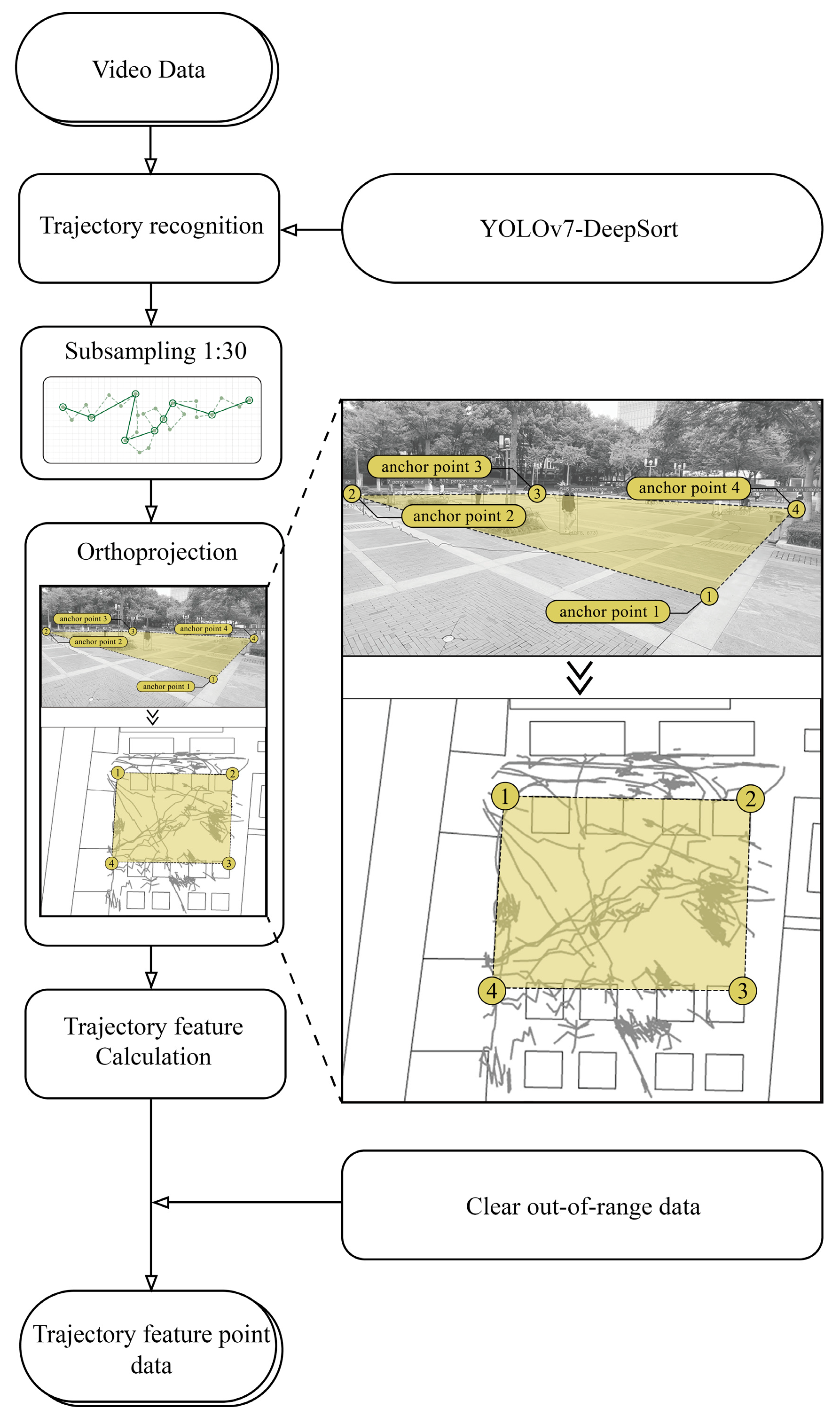
2.3.2. Obtaining Pedestrian Trajectory Data

Different times, weather conditions, and social and natural factors cause crowd behavior in public open spaces to exhibit heterogeneous characteristics [44,45]. Therefore, we tracked and recorded crowd behavior throughout the day. Through our preliminary research, we identified 08:30–20:30 as the site’s peak activity hours. After 18:30, the site was significantly affected by the sunset, resulting in noticeable changes in the lighting environment, which were inconducive to stable crowd data collection. Regarding weather conditions, conducting the data collection on cloudy days was advantageous for reducing the impact of hard-to-measure weather changes on crowd behavior data. Ultimately, we collected the research data at Daxing Palace Square from 08:30 to 18:30 on 18 July 2023. Recordings were taken every hour, and each recording lasted for 5 min.

We established six filming locations at Daxing Palace Square (Figure 5) to cover the primary areas of crowd activity. We used smartphones mounted on 1.7 m tripods for synchronized filming, with the standard video resolution of 1080 p and a frame rate of 30 fps. We used the YOLOv7-DeepSort model to recognize crowd trajectories frame by frame in the video data. Compared with the traditional YOLOv5 model, this model exhibits superior efficiency and accuracy, aiding researchers in obtaining high-confidence crowd trajectory data in large quantities. To smooth the trajectory data, we conducted multiple comparative experiments and decided on a 1:30 ratio for secondary trajectory sampling (Figure 6). Finally, we orthographically projected the crowd trajectories based on predefined landmarks in the frames, resulting in crowd trajectory data being obtained for the subsequent calculations.

To ensure that the separately collected behavioral data did not overlap during the integration, we defined the shooting ranges for each collection point and removed the behavior point data that exceeded these ranges during post-processing. We performed this step after computing the behavioral data characteristics to ensure that each trajectory feature point was calculated in the dataset and to avoid errors caused by data cleaning. Simultaneously, we resolved the trajectory discontinuity issues at the edges of the imagery frames.

We obtained consent from the park management unit for the data collection. During filming, we used eye-catching filming equipment and signs to inform those present that their behaviors were being recorded. All image data were silenced and were only used during the research process.

2.4. Spatial Vitality Factors

2.4.1. Crowd Heat

According to Gehl, spatial vitality can be measured using the number of people in a space and their staying times [17]. Previous studies have defined staying time as the average length of the complete trajectories of different identifications (IDs) within the same period [29]. However, in complex environments with dense crowds, inevitable occlusions can lead to errors in corresponding trajectory IDs [39], significantly reducing the accuracy of staying time measurements. Therefore, we proposed a crowd heat factor, with discrete trajectory feature point data as the statistical unit, to calculate the total number of people present per second in a space (1) and their staying times in that space as follows:

$$H_k=\frac{\sum _{i=0}^n{h}_i}{M_k}$$

(1)

where $H_k$ represents the crowd heat of space k, $h_i$ represents the number of people in sample frame $i$, and $M_k$ represents the area size of space k (m²).

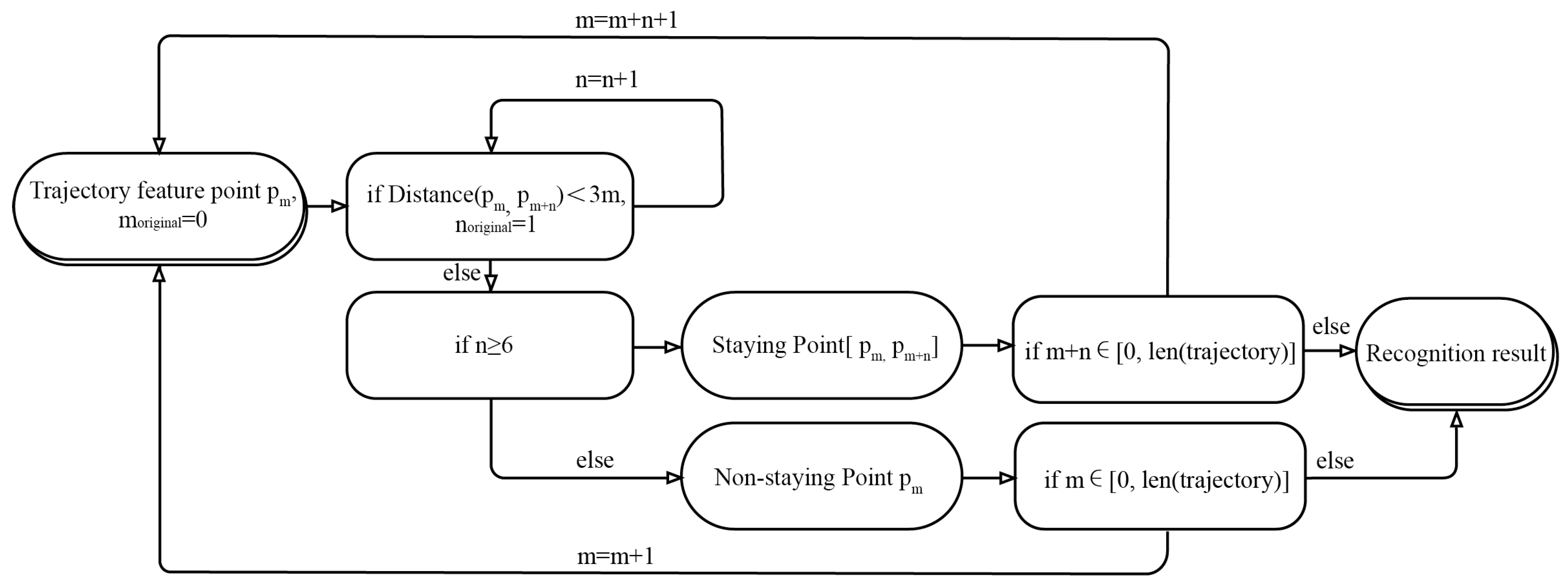
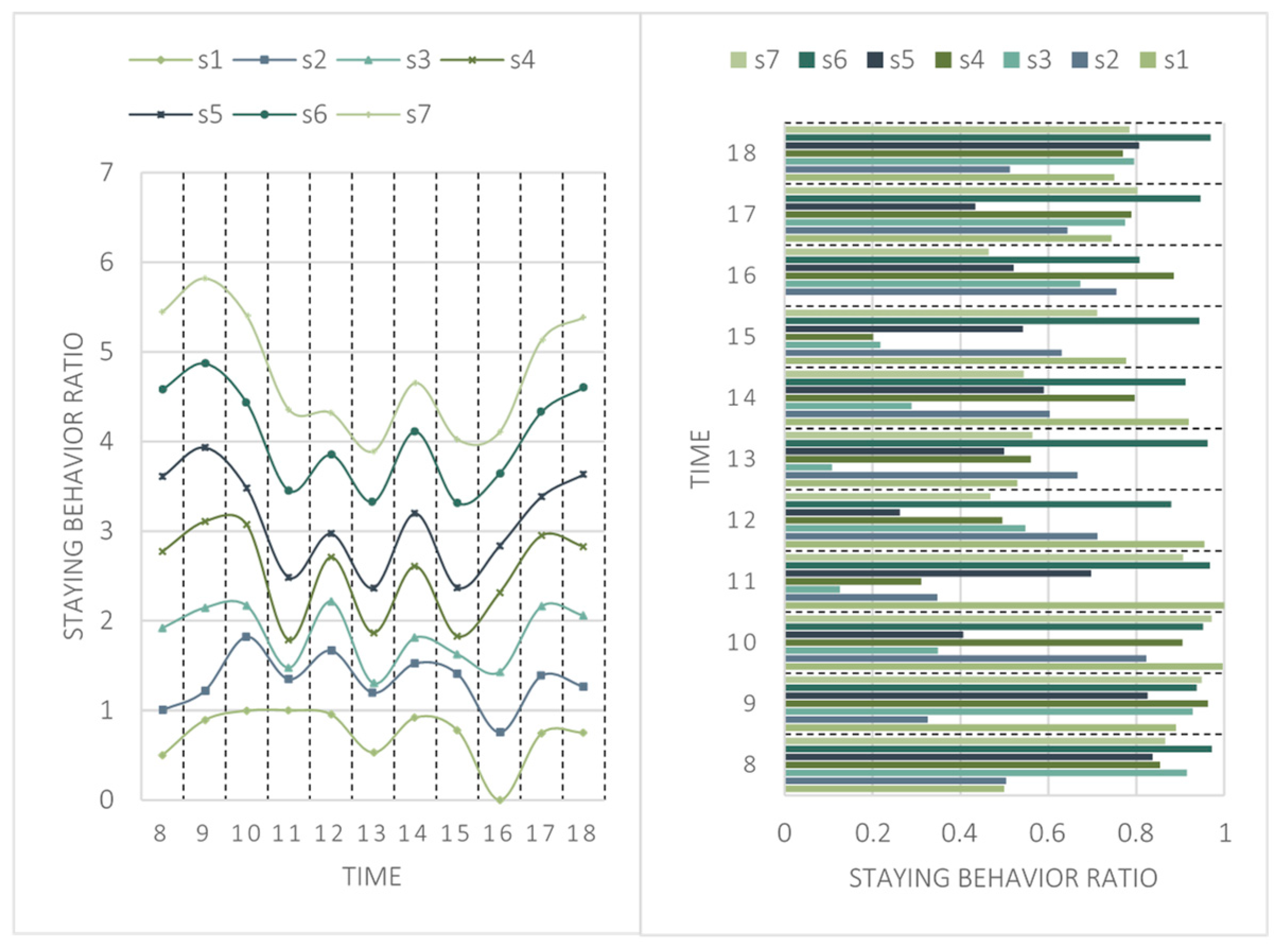
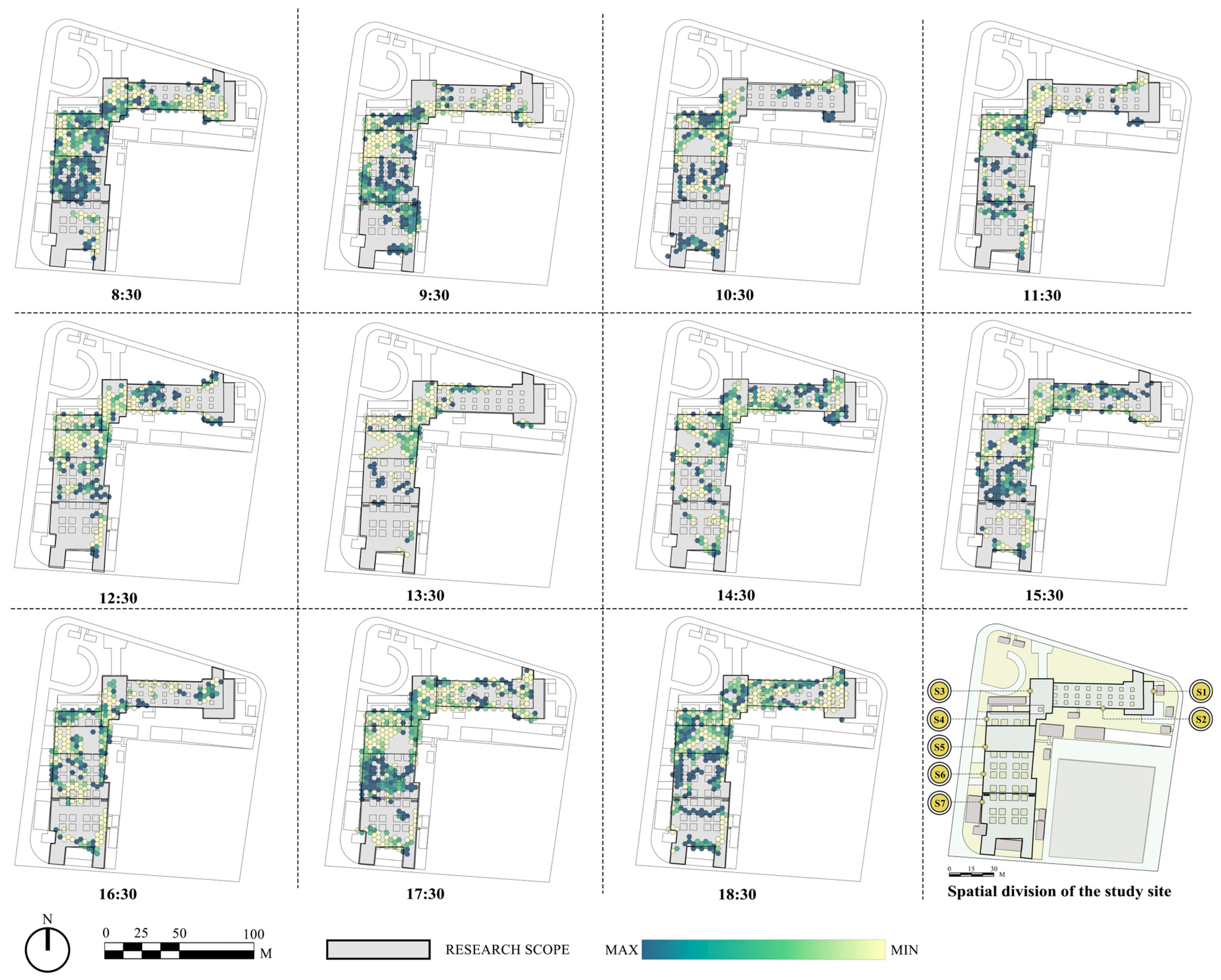
2.4.2. Staying Behavior Ratio

We defined staying behavior as a person remaining within a defined area for a certain period, excluding activities such as running and walking. Previous research has shown that the frequency of staying behavior is a significant indicator of a space’s attractiveness [46]. Public open spaces with high staying behavior frequency tend to generate crowd aggregation effects and social activities, thereby enhancing their spatial vitality. Moreover, distinguishing between non-staying and staying behaviors can assist researchers in better differentiating the impacts of different crowd trajectory types on a space’s spatial vitality. Consequently, we utilized the following method for identifying staying behavior trajectory feature points and formulated identification criteria based on site observations: if a trajectory was within a 3 m radius for ≥6 s (Figure 7), we considered it a staying behavior trajectory.

Finally, we calculated the proportion of staying behavior at a space in a period using the following formula:

$${SP}_k=\frac{{sc}_k}{{pc}_k}$$

(2)

where ${SP}_k$ represents the proportion of the staying behavior in space k, ${sc}_k$ represents the total number of temporal staying behavior trajectory feature points in space $k$, and ${pc}_k$ represents the total number of temporal trajectory feature points in space $k$.

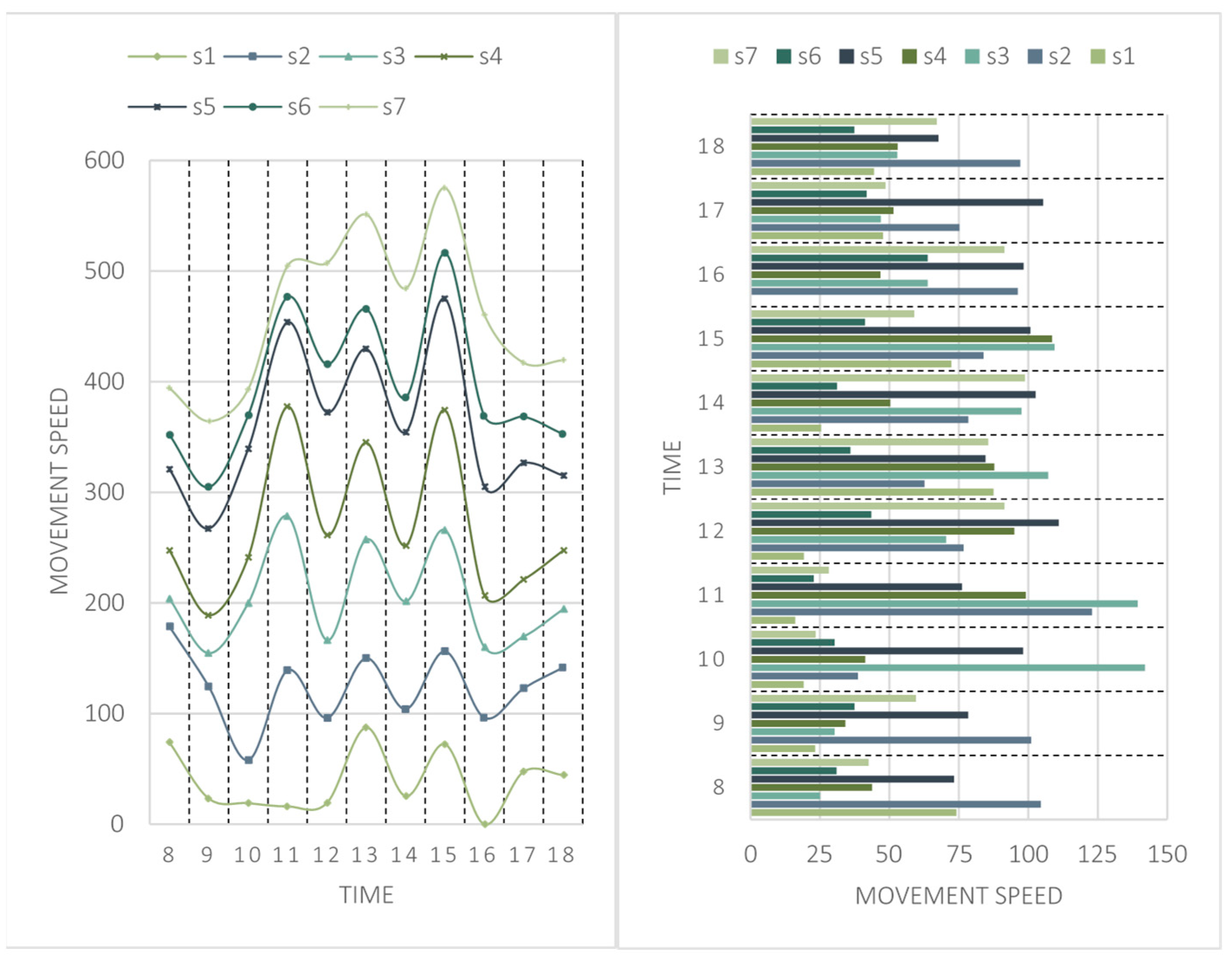
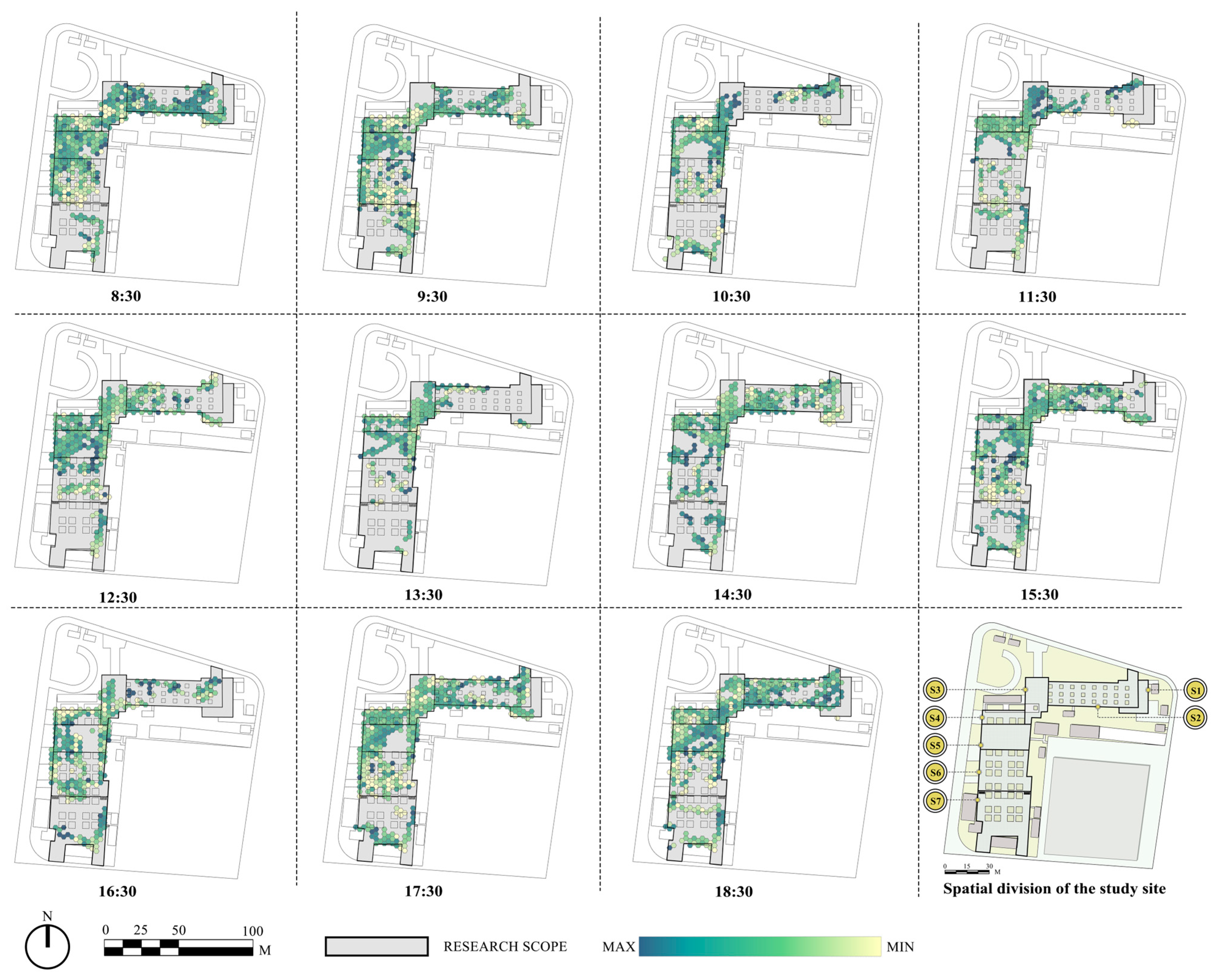
2.4.3. Movement Speed

Movement speed is a crucial dimension of measuring human activity in a space. When integrated with the results of staying behavior recognition, the movement speed of staying behaviors indicates the intensity of human activities, while the movement speed data for non-staying behaviors represents the transit speed of individuals. The former directly reflects spatial vitality, whereas the latter indicates a space’s attractiveness. High-quality vibrant spaces encourage people to slow down and linger [45]. Therefore, we considered movement speed as a factor that represented spatial vitality. To obtain quantitative values for this factor, we calculated the Euclidean distance between adjacent trajectory feature points with the same ID to represent the movement distance per second (3) and the average movement speed for each space within a specific period (4) as follows:

$$S_{p_i}=\left\{\begin{array}{c}\frac{{‖\overrightarrow{p_i{p}_{i+1}}‖}_2}{t},i\in \left[0,len\left(tr\right)\right)\cap i\in Z\\ {SP}_{p_{i-1}},i=len\left(tr\right)\end{array}\right.$$

(3)

$${AS}_k=\frac{\sum _{i=0}^n{S}_{p_i}}{\sum _{i=0}^n{h}_i}$$

(4)

where $S_{pi}$ represents the movement speed of trajectory feature point $p_i$, $t$ represents the sampling interval between two trajectory feature points, and $len\left(tr\right)$ represents the total number of samples for a trajectory. ${AS}_k$ represents the average movement speed for space $k$ within a specific period. The movement speed of the last trajectory feature point is the same as that of the second to last point.

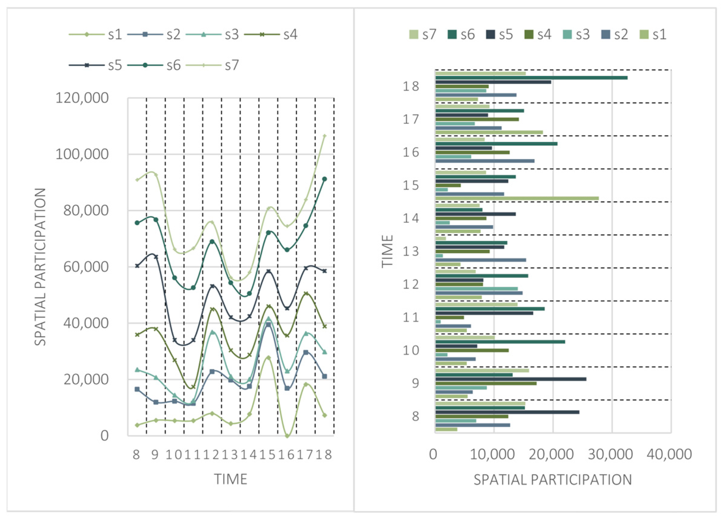
2.4.4. Spatial Participation

We defined spatial participation as the extent to which human behavior was influenced by environmental or social forces within a space. Regarding crowd behavior, using space as a conduit for transportation results in a simple trajectory structure. In contrast, behaviors such as sitting, sightseeing, dancing, and others exhibit complex trajectory structures, indicating that these behaviors are subject to environmental or social forces to a greater extent [47]. This suggests people’s deep participation in space, thereby enhancing spatial vitality. Therefore, we utilized quantifiable trajectory structures to characterize people’s spatial participation and aid our examination of spatial vitality.

Regarding the quantification of the trajectory structures, structural differences exist for different trajectories, and structural differences also exist among the local structures within the same trajectory. However, most of the extant methods for determining trajectory structures can only assess the structure of complete trajectories; as such, they neglect the specificity of local structures within the same trajectory [29]. To enhance the representational capability of structural difference indicators for local trajectory segments, we used a structural difference calculation method based on distance and rank weighting and assigned structural difference values to trajectory feature points $p_i$ as follows: First, we introduced the trajectory length difference (5) and trajectory angle difference (6), whose effectiveness has been demonstrated in prior research.

$$D_{p_i}=\left\{\begin{array}{c}\left|{‖\overrightarrow{p_{i-1}{p}_i}‖}_2-{‖\overrightarrow{p_i{p}_{i+1}}‖}_2\right|,i\in \left(0,len\left(tr\right)\right)\cap i\in Z\\ D_{p_{i+1}},i=0\\ D_{p_{i-1}},i=len\left(tr\right)\end{array}\right.$$

(5)

$$A_{p_i}=\left\{\begin{array}{c}{\mathit{cos}}^{-1}\left(\frac{\overrightarrow{p_{i-1}{p}_i}·\overrightarrow{p_i{p}_{i+1}}}{{‖\overrightarrow{p_{i-1}{p}_i}‖}_2{‖\overrightarrow{p_i{p}_{i+1}}‖}_2}\right),i\in \left(0,len\left(tr\right)\right)\cap i\in Z\\ A_{p_{i+1}},i=0\\ A_{p_{i-1}},i=len\left(tr\right)\end{array}\right.$$

(6)

where $D_{p_i}$ represents the trajectory length difference, $A_{p_i}$ represents the trajectory angle difference, and the length and angle differences between the initial and final trajectory feature points are the assigned values of the adjacent trajectory feature points. Subsequently, we calculated the weighted values (7) for the trajectory feature points based on the rank and distance differences, which were weighted using Gaussian functions:

$$W_{p_{ij}}=e^{\frac{{d^2(p_i,p_j)·dist}^2(p_i,p_j)}{4c_r^2·c_l^2}}$$

(7)

where $W_{p_{ij}}$ represents the weight of trajectory feature point $p_j$ relative to $p_i$, $d(p_i,p_j)$ denotes the rank difference between trajectory feature points, $dist(p_i,p_j)$ signifies the Euclidean distance between trajectory feature points, and $c_r$ and $c_l$ are the Gaussian weighting functions for the rank and Euclidean distance, respectively. We set $c_r$ as 3 and $c_l$ as 150, which was half of the threshold value for determining staying behavior. We considered the trajectory feature points that were further apart in rank and Euclidean distance to have relatively low weights, indicating low interrelatedness. Subsequently, we calculated the spatial participation (${SC}_{p_i}$) (8) based on Formulas (5)–(7). We then obtained the temporal average of the spatial participation in space $k$ (${AC}_k$) (9) as follows:

$${SC}_{p_i}={\displaystyle {\sum }_{j=0}^n}{D}_{p_j}{A}_{p_j}{W}_{p_{ij}}$$

(8)

$${AC}_k=\frac{\sum _{i=0}^n{SC}_{p_i}}{\sum _{i=0}^n{h}_i}$$

(9)

2.5. Manual Assessment of Spatial Vitality

Manual assessment is the mainstream method used to evaluate the effectiveness of machine monitoring and has been widely applied in various urban research fields [43], providing a humanistic research perspective. Currently, many indicators are used to evaluate spatial vitality [48]; however, different indicator types are prone to interference, affecting the evaluation results. Therefore, it was necessary to formulate a set of unified standards to evaluate the spatial vitality, provide training to experts, and standardize the theoretical basis of the evaluation results. Since we defined our aforementioned indicators to accommodate machine detection, they differed from those used in human assessments. Therefore, we adjusted the indicator definitions to align them with manual scoring conventions. Moreover, the indicators to be manually assessed were consistent with those used in machine monitoring in terms of their evaluation dimensions, allowing for the performance assessment of machine-monitored spatial vitality in the spatiotemporal dimensions. Finally, we utilized a set of spatial vitality evaluation standards composed of four sub-indicators: crowd heat, staying behavior ratio, movement speed, and spatial participation.

2.6. Assessment Criteria

2.6.1. Crowd Heat

We defined crowd heat as the total number of people present in a space per second during the video capture. Large transient crowds and small stationary crowds can provide equivalent crowd heat [17]. Therefore, we graded crowd heat using five levels (

Table 2. Crowd heat rating rules.

Grade	Description
1	Few people
2	Relatively few people
3	Moderate number of people
4	Relatively many people
5	Many people

). Subsequently, 13 experts with backgrounds in urban and rural planning and landscape architecture volunteered to conduct manual assessments of the spatial vitality. The experts used their professional knowledge to determine the two crowd types’ contributions to crowd heat and provide comprehensive scores. The experts focused on the independence of crowd heat as a spatial vitality factor and avoided interference from other crowd behavior characteristics.

2.6.2. Staying Behavior Ratio

We defined stationary behavior as a person remaining in a space for more than 6 s, including standing, resting, and activities, such as games and fitness. We graded the occurrence of stationary behavior in a space using five levels (

Table 3. Staying behavior ratio rating rules.

Grade	Description
1	Almost all crowd behaviors are non-staying
2	Most crowd behaviors are non-staying, and more than half of the staying people have short stay times (less than 1 min)
3	Most crowd behaviors are non-staying, with more than half of the staying people having longer stay times (over 1 min); most crowd behaviors are staying, and more than half of the staying people have shorter stay times (less than 1 min)
4	Most crowd behaviors are staying, and more than half of the staying people have longer stay times (over 1 min)
5	Almost all crowd behaviors are staying

). Because human observation cannot replicate machine precision, we required the experts to watch video clips repeatedly until they reached a consensus in the pre-scoring.

2.6.3. Movement Speed

We defined movement speed as the crowd’s movement speed. Unlike the machine monitoring indicators, we used walking speed to refer to the distance that a person covered in a space within a certain period, rather than the displacement distance per second. This was because excessively detailed observation requirements would reduce the accuracy of human judgments. We graded movement speed using five levels based on the average movement speed of the crowd in a space (

Table 4. Movement speed rating rules.

Grade	Description
1	Most crowd behaviors have slow movement speeds
2	Most crowd behaviors have relatively slow movement speeds
3	The proportion of crowd behaviors with different movement speeds is balanced
4	Most crowd behaviors have relatively fast movement speeds
5	Most crowd behaviors have fast movement speeds

).

2.6.4. Spatial Participation

Machine monitoring quantifies the structure of a trajectory, representing the interaction status of crowd behavior with both a space and other crowds. While a manual assessment cannot accurately assess the state of trajectory structure, the determination of fuzzy details, such as social behavior, upper body movements, and facial expressions, is an advantage of this method. We graded spatial participation using five levels based on the crowd behaviors in a space (

Table 5. Spatial participation rating rules.

Grade	Description
1	Most crowd behaviors have weak interactions with space, with few or no social behaviors
2	Most crowd behaviors have moderate interactions with space, with relatively few social behaviors
3	Most crowd behaviors have moderate interactions with space, with a moderate number of social behaviors
4	Most crowd behaviors have strong interactions with space, with relatively many social behaviors
5	Most crowd behaviors have strong interactions with space, with many social behaviors

).

2.7. Validation Process

We designed a standardized process for the manual assessment and subsequent validation of the results to ensure the credibility of the results. First, considering the manual assessment’s high workload, we selected five typical periods as the evaluation samples—8:30, 10:30, 12:30, 15:30, and 18:30—to represent the variations in spatial vitality throughout the day. We then established the following workflow for the manual assessment.

2.7.1. Preparation Phase

We briefed the experts on the experimental procedures and provided scoring instructions, sample videos, and a platform on which to seek clarification. As a single video could include images from multiple spatial locations, we informed the experts in advance about the specific ranges of each space within each video to prevent interference from other spaces in the scoring.

2.7.2. Pre-Scoring Phase

We selected the video data from 09:30 as the training sample. The experts completed two full viewings of the video from spaces S1 to S7 and then scored each evaluation indicator. Subsequently, we used the widely accepted intraclass correlation coefficient (ICC) to verify the scoring effectiveness [49]. This process was repeated until it passed the reliability test. As the scoring results were derived from a randomly sampled infinite dataset using a single method, the ICC used a two-way random model for the single rater type. We also used the absolute agreement type to consider systematic errors among the raters and monitor the potential for different individual raters to overestimate or underestimate the spatial vitality factor assessment.

2.7.3. Scoring Phase

To prevent scoring errors due to the order of video viewing, the experts initially scored each indicator and space for the five sample periods. They then repeated the viewing process. During this time, they could adjust their scores. Once completed, the scoring results were subjected to ICC reliability testing. The ICC model used was consistent with that used in the prescoring phase.

2.7.4. Validation Phase

We employed ICC to assess the consistency between the human and machine monitoring scores, which were standardized using min.–max. normalization. Since the scoring for this phase was based on a random sample from an infinitely large sample set, the ICC used a two-way random model with a single rater type. To investigate the presence of systematic errors between the human and machine monitoring scores, we compared the results using two ICC models: absolute agreement and consistency (

Table 6. ICC scores.

Spatial Vitality Indicators	Human Evaluation Agreement (Absolute Agreement)		Machine Monitoring vs. Human Evaluation (Absolute Agreement)		Machine Monitoring vs. Human Evaluation (Consistency)
	ICC	p	ICC	p	ICC	p
Crowd heat	0.763	<0.001	0.512	<0.001	0.719	<0.001
Staying behavior ratio	0.820	<0.001	0.549	<0.001	0.812	<0.001
Movement speed	0.794	<0.001	0.612	<0.001	0.628	<0.001
Spatial participation	0.748	<0.001	0.584	<0.001	0.660	<0.001

Note. ICC > 0.8 denotes perfect agreement, 0.6 < ICC < 0.8 denotes substantial agreement, 0.4 < ICC < 0.6 denotes moderate agreement, 0.2 < ICC < 0.4 denotes fair agreement, and ICC < 0.2 denotes slight agreement; p < 0.001 suggests statistical significance [50].

).

3. Results

3.1. Validation Results

Table 6 shows that for the intergroup consistency model using human evaluation, the ICC values for all indicators exceed 0.6, showing substantial agreement or higher. This indicates the high reliability of the spatial vitality scores obtained through human evaluation.

Regarding the intergroup consistency between machine monitoring and human evaluation using the absolute agreement model, the values for crowd heat, resident behavior ratio, and spatial participation range from 0.4 to 0.6, indicating moderate agreement. The ICC values for movement speed range from 0.6 to 0.8, signifying substantial agreement. The consistency ICC model values range from 0.6 to 0.8 for all indicators, also indicating substantial agreement. The ICC values for crowd heat, staying behavior ratio, and spatial participation under the consistency model are significantly higher, while those for movement speed are similar in both models. This may be because counting, comparing ratios, and distinguishing different behaviors require cognitive effort and memory, making it difficult for people to make effective judgments in adjacent situations and leading to conservative estimations with significant systematic biases. Movement speed can be scored in a way that aligns with human perceptions of everyday speeds, such as “no displacement”, “slow walking”, “normal walking”, “fast walking”, and “jogging”, resulting in more objective scoring with less systematic bias. This further validates the advantages of our machine monitoring approach in terms of objectivity and precision in the spatial vitality assessment of the study site.

3.2. Spatial Vitality Factor Analysis

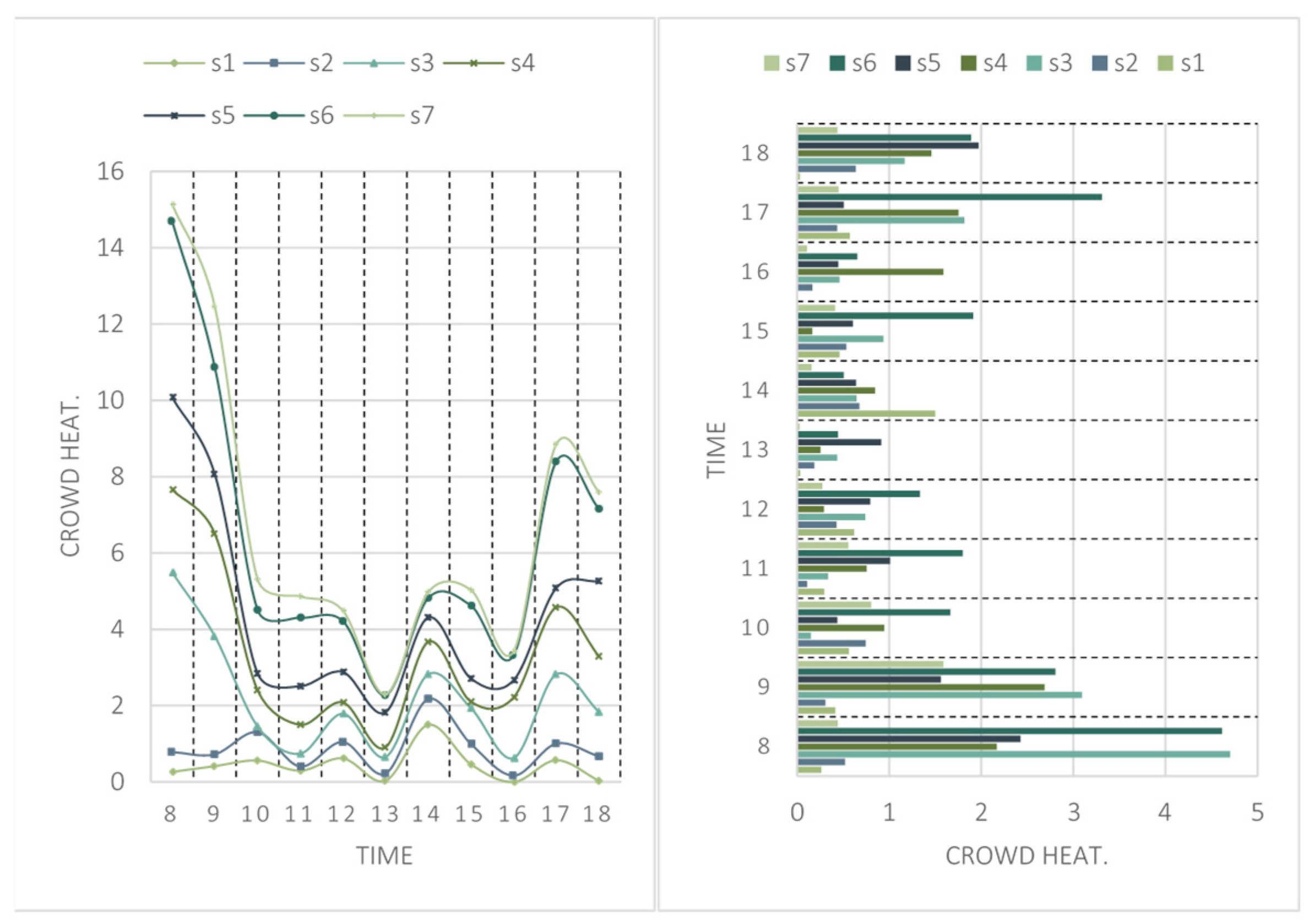
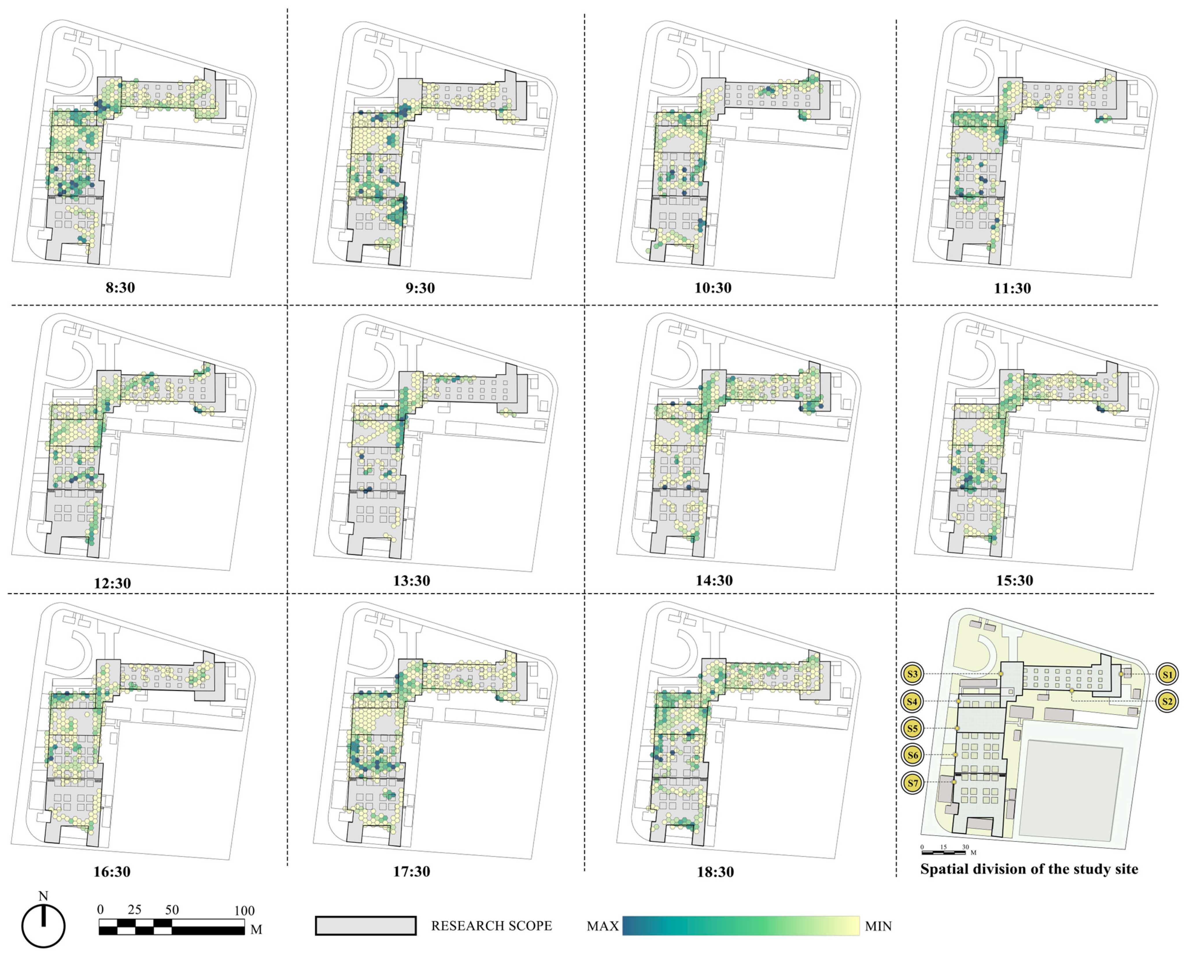
3.2.1. Crowd Heat

Figure 8 (left) shows that crowd heat peaks at 08:30 and 17:30 and troughs at 13:30, showing a pattern of low in the middle and high on both sides. The temporal trends of crowd heat in various spaces are generally consistent with the overall study site, with peaks at the 08:30–10:30 and 17:30–18:30 periods and troughs at the 12:30–14:30 period.

Figure 8 (right) shows that crowd heat in s4 and s6 maintains relatively high values throughout the period, demonstrating the significant advantage of spaces with large enclosures in attracting crowd activity. S3 and s5, with lower enclosures, demonstrate the highest crowd heat values at 08:30 and 18:30, respectively. This may be because collective sports, children’s play, and social activities were performed at 08:30 and 18:30, and these activities utilized the hard surfaces provided by the spaces with low enclosures. S2, also characterized by a low enclosure, experiences low crowd heat values throughout the period owing to the disruption in spatial continuity caused by the array of tree pits. The spatial distribution map (Figure 9) confirms the aforementioned observations, with high-frequency crowd distributions occurring in high-enclosure spaces or at landscape boundaries throughout the period. From 08:30 to 9:30 and from 17:30 to 18:30, the crowd distributions occur synchronously in low-enclosure spaces with good spatial continuity.

3.2.2. Staying Behavior Ratio

Figure 10 (left) shows that the staying behavior ratio peaks at 09:30, decreases from 09:30 to 11:30, stabilizes before 16:30, and increases from 16:30 to 18:30. Overall, the staying behavior ratio exhibits a U-shaped distribution pattern, with higher values in the morning and evening and lower values at midday.

Regarding the spatial distribution, Figure 10 (right) shows that the proportion of staying behavior in s6 exceeds 0.8 throughout the period, whereas other spaces exhibit larger fluctuations. Specifically, the amplitude in s3 reaches 0.82. This may be attributed to the high-enclosure nature of and excellent rest facilities in s6, which enhance its attractiveness for staying behavior. However, this does not imply that low-enclosure spaces have a negative impact on staying time. Influenced by aggregative crowds, such as square dancing, the staying behavior ratio value in s3 at 08:30 is second only to that of s6. Additionally, there is a clustering phenomenon of staying behavior at the landscape boundaries for various spaces, which is consistent with the “boundary effect” theory (Figure 11) [17].

3.2.3. Movement Speed

Figure 12 (left) shows that the movement speed peaks at 15:30 and troughs at 9:30, exhibiting an overall camel-shaped distribution, with higher values at midday and lower values in the morning and evening, showing a negative correlation with other feature factors.

Figure 12 (right) shows similar fluctuation trends for the movement speed in various spaces. S3, s5, and s7 maintain relatively higher movement speeds throughout the period, whereas s4 and s6 exhibit lower movement speeds, suggesting a preference for high-speed behavior in low-enclosure spaces. Figure 13 shows that high-speed movement areas exhibit extensive clustering, particularly at 17:30, when continuous clusters appear in s2, s3, and s5. Low-speed movement areas mostly display isolated point-like distributions at the landscape boundaries. Additionally, low-speed movement areas in s3 exhibit clustered distributions, whereas those in s6 mostly show scattered distribution patterns and the phenomenon of intermittent high-speed behaviors. This suggests that low-density, low-speed behaviors tend to occur in high-enclosure spaces with better rest facilities, whereas high-density, low-speed behaviors, represented by square dancing, tend to occur in low-enclosure spaces.

3.2.4. Spatial Participation

Figure 14 (left) shows that the spatial participation fluctuates periodically, reaching a trough at 13:30 and experiencing significant growth from 14:30 to 18:30. Owing to the absence of crowd behavior data in s1, there is no spatial participation at 16:30, resulting in an overall decrease in spatial participation. Overall, the temporal distribution of spatial participation exhibits a U-shaped pattern, with higher values in the morning and evening and lower values at midday.

Figure 14 (right) shows that the spatial participation value in s5 is higher than that in other spaces from 08:30 to 09:30 due to the influence of morning exercise behavior. In other periods, s6 consistently leads in its spatial participation value. Figure 15 shows that at 17:30, s3 and s6 form large-scale clusters of low- and high-level spatial participation, respectively, reflecting differences in crowd behavior in spaces with distinct characteristics. In s3, the crowd behavior is passage-oriented, whereas in s6, crowds tend to engage in extensive interactions with the space. This aligns with the evaluations of other spatial vitality factors. Therefore, despite the relatively high levels of crowd heat in s3 and s6 at 17:30 (Figure 14 (left)), the spatial vitality values exhibit significant differences. Furthermore, from 08:30 to 09:30 and from 11:30 to 17:30, there is a clustering phenomenon of high-level spatial participation at the eastern boundary of s5, while isolated high-participation aggregation areas appear at the tree pool boundary of s1 from 10:30 to 17:30 (Figure 15). In other periods, the distribution of high- and low-participation crowd behavior is mixed, but high-participation areas are generally shown at the boundaries of high-enclosure spaces and landscape boundaries (Figure 15), possibly indicating that in-depth interactions between people and spaces are more likely to occur at spatial boundaries, which correlates with the tendency to exhibit staying behavior at boundaries.

4. Discussion

We utilized a CV-supported method for spatial vitality detection and conducted a spatiotemporal statistical analysis of a small site’s vitality. Compared with manual counting [34] or the results obtained from continuous trajectories [29], we quantitatively determined the spatial coordinates and temporal sequences of crowd behavior per second, thus enhancing the efficiency and reliability of the spatial vitality assessment indicators. Moreover, by using fine-grained behavioral data, we conducted a multidimensional behavioral factor assessment of spatial vitality at an appropriate scale so as to address the criticism of single-factor spatial vitality assessment subjectivity [38] and enhance the feasibility of examining the coupling between spatial vitality and spatial features in small-scale space research.

Regarding the behavioral data, we transformed continuous behavioral trajectories into discrete multidimensional behavior trajectory feature points to efficiently expand the dataset volume, reduce the impact of erroneous data, and enhance the granularity of the behavioral data. Simultaneously, our method of overlapping different viewpoints using the weighted calculations of the behavioral features in the original dataset, and our subsequent use of spatial segmentation, effectively resolved the trajectory discontinuity issues at the edges of the imagery frames [41]. The manual assessment results demonstrated that the behavior feature calculation based on discrete trajectory feature points could characterize the various spatial vitality factors. However, we noticed that the tracking loss problems persisted owing to the occlusion of the camera view, behaviors being too far from the camera equipment, or behaviors extending beyond the cameras’ coverage boundaries. This resulted in the loss of some data on crowd behavior. Our feasibility analysis demonstrated that the use of discrete trajectory feature point data to expand the dataset ensures that minor data losses do not affect the measurement of spatial vitality factors. Nevertheless, if video datasets with high camera view occlusion rates are used, or if the camera positions in the research site cannot cover the entire area, the accuracy of the spatial vitality measurement results cannot be guaranteed. Therefore, as with other studies that use video data, the quality of the video data is important.

Regarding the correlation between spatial vitality and spatial features, our experimental results had strong explanatory power for the “boundary effect” theory [17], indicating a significantly positive impact of landscape boundaries on spatial vitality phenomenon. This was deduced through our statistical analysis of the spatial vitality factor calculations and spatial vitality distribution maps supported by discrete trajectory feature point data. We found that the landscape boundary regions significantly and positively impacted the spatial vitality factors, which is consistent with Loo et al.’s results [40]. Moreover, our results indicated that the spatial vitality factors were not solely influenced by the landscape boundaries; spatial characteristics, such as the continuity of hard-surfaced spaces, rest facilities, and enclosure levels, also had complex nonlinear influencing effects. Therefore, future research should use a nonlinear multivariate quantification model to explore the correlation between spatial features and spatial vitality.

Our study has a few limitations. Regarding the research site, first, the data used in this study were collected from a specific public open space in Nanjing, China. While this does not affect the credibility of the spatial vitality monitoring results, the findings on the temporal variation patterns of spatial vitality and its correlation with spatial features may not be generalizable to other cities and regions with different geographical and cultural backgrounds [51]. Secondly, since the purpose of this study was to explore a feasible method for the automated multi-dimensional monitoring of public open space vitality at a small scale, we chose a city square that is rich in spatial types and activity categories for method testing. In our future work, we will aim to explore the applicability of this method in different types of public open spaces. Moreover, in different types of public open spaces, more trajectory features may need to be considered. For instance, in a commercial street space, the trajectory features generated by the interaction between crowds and surrounding shops might be an important variable in spatial vitality monitoring, while in mountainous parks, changes in trajectory on the z-axis will become one of the trajectory features we need to consider.

In terms of the selection of spatial features, further research into the nonlinear correlation between spatial features and spatial vitality, as mentioned in the previous discussion, will require the fine-grained quantification of spatial features and more potentially relevant spatial features. For example, Wei et al. [41] qualitatively discussed the “tele-coupling” phenomenon, which suggests that spatial features outside the research site may influence crowd behavior within the site, yet there is no method available for effective quantitative discussion. Moreover, if the spatial vitality monitoring method proposed in this paper were to be extended to studies of other types of public open spaces, more spatial features suited to the research subject would need to be considered. For instance, in urban street spaces, interface shapes and facade elements have been reported as important spatial features [16]. In urban parks with environments that are more complex than that of the research site of this study, natural spatial features, such as bodies of water and lawns, as well as artificial spatial features, like sculptures, fountains, and fitness equipment, need to be taken into consideration [30]. Our future work includes exploring methods to create a quantitative representation of spatial features to advance the quantitative study of the relationship between spatial features and spatial vitality in small-scale public open spaces.

Furthermore, we recognized that the nature of our sampling research could lead to the presence of errors. Our sampling periods covered the major activity periods of the day and met the accuracy requirements for conducting temporal change research. However, weather and lighting conditions, which are significant influencing factors of spatial vitality, change rapidly. Limited by current technological capabilities, we struck a balance between sampling time and efficiency and selected cloudy weather to mitigate the impact of lighting conditions. However, we again acknowledged the potential existence of sampling errors. When more efficient video collection and behavior tracking methods become available, continuous behavior monitoring throughout the day can replace our sampling approach and enhance the accuracy of spatial vitality research in the future.

5. Conclusions

Determining and analyzing the vitality of public open spaces is crucial for urban planners and designers to understand the use of such spaces and enhance their functionality, along with the support of CV technology to enable efficient quantitative data collection. Based on our behavioral data characteristics and the spatial vitality assessment, we transformed the behavioral data into four multidimensional spatial vitality factors, namely crowd density, staying behavior ratio, movement speed, and spatial participation, and analyzed their spatiotemporal distribution in Daxing Palace Square. Our study contributions are outlined below.

First, our use of discrete trajectory feature points reduced the data collection errors and helped us calculate the spatial vitality factors, which effectively addressed the data sensitivity issues arising from trajectory fragmentation and inadequate sample sizes between different data collection ranges. Therefore, our constructed spatial vitality monitoring model and vitality distribution maps avoided interference from duplicate data or blank areas. Second, by leveraging the advantages of discrete trajectory feature points in the subdivision of the behavioral feature space, we constructed spatial vitality maps that showed that all four spatial vitality factors exhibited positive characteristics at the landscape boundaries, which is consistent with Gehl’s “boundary effect” theory [17], indicating that landscape boundaries have a significantly positive impact on spatial vitality. Third, we simultaneously quantified the changing trends in spatial vitality factors at different periods. From 08:30 to 09:30 and from 17:30 to 18:30, the crowd heat and staying behavior ratio values in the square were higher, and the crowd movement speed value was lower, indicating people’s greater tendency to engage with the square space at these times. Spatially, this phenomenon was more prominent in the high-enclosure areas of s4 and s6. Finally, we examined the complex coupling relationship between spatial features and spatial vitality. The analysis revealed that better rest facilities consistently and positively impacted spatial vitality. High-enclosure spaces were more likely to attract more spatial participation behaviors, increasing the interactions between people and spaces. Conversely, low-enclosure spatial features attracted high- and low-speed aggregative behaviors, negatively impacting the staying behavior ratio and spatial participation behaviors. Overall, high-enclosure areas positively impacted spatial vitality, while low-enclosure areas exhibited higher spatial vitality during periods of concentrated aggregative behavior.

The multidimensional spatial vitality automated monitoring method proposed in this article is a standardized and scalable workflow. In urban research, it addresses the challenge of quantitatively analyzing spatial vitality at the human scale, assisting urban researchers in examining the spatiotemporal distribution and influencing factors of vitality in public open spaces across multiple dimensions and scales and summarizing patterns from it. In the context of urban design and renovation, the method developed in this paper can assist designers in making quantitative assessments of the temporal and spatial differences in current spatial vitality. Furthermore, the spatial vitality recorded by discrete trajectory feature points can be conveniently chosen for analysis granularity and overlaid with other urban data for targeted urban space renovation. Designers can also quantitatively compare changes in spatial vitality before and after renovations, serving as scientifically backed material for design retrospectives.

References

1. Ren, X. Combined effects of dominant sounds, conversational speech and multisensory perception on visitors’ acoustic comfort in urban open spaces. Landsc. Urban Plan. 2023, 232, 104674. [Google Scholar] [CrossRef]
2. Scheiber, S. Re-designing urban open spaces to act as green infrastructure—The case of Malta. Transp. Res. Procedia 2022, 60, 148–155. [Google Scholar] [CrossRef]
3. Hooper, P.; Boruff, B.; Beesley, B.; Badland, H.; Giles-Corti, B. Testing spatial measures of public open space planning standards with walking and physical activity health outcomes: Findings from the Australian national liveability study. Landsc. Urban Plan. 2018, 171, 57–67. [Google Scholar] [CrossRef]
4. Wang, A.; Ho, D.C.W.; Lai, L.W.C.; Chau, K.W. Public preferences for government supply of public open space: A neo-institutional economic and lifecycle governance perspective. Cities 2023, 141, 104463. [Google Scholar] [CrossRef]
5. Mu, B.; Mayer, A.L.; He, R.; Tian, G. Land use dynamics and policy implications in Central China: A case study of Zhengzhou. Cities 2016, 58, 39–49. [Google Scholar] [CrossRef]
6. Zheng, W.; Shen, G.Q.; Wang, H.; Hong, J.; Li, Z. Decision support for sustainable urban renewal: A multi-scale model. Land Use Policy 2017, 69, 361–371. [Google Scholar] [CrossRef]
7. Xie, D.; Fan, J.; Chang, J. From space reproduction to place-making: The new trend of China’s urban regeneration. Urban Dev. Stud. 2017, 24, 110–115. [Google Scholar]
8. Ma, L.; Shi, W.; Wu, L. Mediating roles of perceptions and visiting behavior in the relationship between urban greenspace accessibility and personal health: Evidence from Lanzhou, China. Appl. Geogr. 2023, 159, 103085. [Google Scholar] [CrossRef]
9. Xia, H.; Yin, R.; Xia, T.; Zhao, B.; Qiu, B. People-Oriented: A Framework for Evaluating the Level of Green Space Provision in the Life Circle from a Supply and Demand Perspective: A Case Study of Gulou District, Nanjing, China. Sustainability 2024, 16, 955. [Google Scholar] [CrossRef]
10. Wang, N.; Zhao, Y. Construction of an ecological security pattern in Jiangnan water network area based on an integrated Approach: A case study of Gaochun, Nanjing. Ecological Indicators 2024, 158, 111314. [Google Scholar] [CrossRef]
11. Chen, J.; Chen, L.; Li, Y.; Zhang, W.; Long, Y. Measuring Physical Disorder in Urban Street Spaces: A Large-Scale Analysis Using Street View Images and Deep Learning. Ann. Am. Assoc. Geogr. 2023, 113, 469–487. [Google Scholar] [CrossRef]
12. Ding, P.; Jensen, F.S.; Carstensen, T.A.; Jorgensen, G. Exploring adults’ passive experience of children playing in cities: Case study of five urban public open spaces in Copenhagen, Denmark. Cities 2023, 136, 104250. [Google Scholar] [CrossRef]
13. Zhu, W.; Wang, J.; Qin, B. Quantity or quality? Exploring the association between public open space and mental health in urban China. Landsc. Urban Plan. 2021, 213, 104128. [Google Scholar] [CrossRef]
14. Jacobs, J. The Death and Life of Great American Cities; Random House: New York, NY, USA, 1961. [Google Scholar]
15. Liu, S.; Lai, S.-Q.; Liu, C.; Li, J. What influenced the vitality of the waterfront open space? A case study of Huangpu River in Shanghai, China. Cities 2021, 114, 103197. [Google Scholar] [CrossRef]
16. Zhang, L.; Zhang, R.; Yin, B. The impact of the built-up environment of streets on pedestrian activities in the historical area. Alex. Eng. J. 2021, 60, 285–300. [Google Scholar] [CrossRef]
17. Gehl, J. Life between Buildings; Van Nostrand Reinhold: New York, NY, USA, 1987. [Google Scholar]
18. Jia, C.; Liu, Y.; Du, Y.; Huang, J.; Fei, T. Evaluation of Urban Vibrancy and Its Relationship with the Economic Landscape: A Case Study of Beijing. Isprs. Int. J. Geo-Inf. 2021, 10, 72. [Google Scholar] [CrossRef]
19. Miranda, A.S.; Fan, Z.; Duarte, F.; Ratti, C. Desirable streets: Using deviations in pedestrian trajectories to measure the value of the built environment. Comput. Environ. Urban Syst. 2021, 86, 101563. [Google Scholar] [CrossRef]
20. Delclos-Alio, X.; Gutierrez, A.; Miralles-Guasch, C. The urban vitality conditions of Jane Jacobs in Barcelona: Residential and smartphone-based tracking measurements of the built environment in a Mediterranean metropolis. Cities 2019, 86, 220–228. [Google Scholar] [CrossRef]
21. Wu, J.; Ta, N.; Song, Y.; Lin, J.; Chai, Y. Urban form breeds neighborhood vibrancy: A case study using a GPS-based activity survey in suburban Beijing. Cities 2018, 74, 100–108. [Google Scholar] [CrossRef]
22. Hahm, Y.; Yoon, H.; Choi, Y. The effect of built environments on the walking and shopping behaviors of pedestrians; A study with GPS experiment in Sinchon retail district in Seoul, South Korea. Cities 2019, 89, 1–13. [Google Scholar] [CrossRef]
23. Sulis, P.; Manley, E.; Zhong, C.; Batty, M. Using mobility data as proxy for measuring urban vitality. J. Spat. Inf. Sci. 2018, 2018, 137–162. [Google Scholar] [CrossRef]
24. Meng, Y.; Xing, H. Exploring the relationship between landscape characteristics and urban vibrancy: A case study using morphology and review data. Cities 2019, 95, 102389. [Google Scholar] [CrossRef]
25. Wu, C.; Ye, X.; Ren, F.; Du, Q. Check-in behaviour and spatio-temporal vibrancy: An exploratory analysis in Shenzhen, China. Cities 2018, 77, 104–116. [Google Scholar] [CrossRef]
26. Yue, W.; Chen, Y.; Zhang, Q.; Liu, Y. Spatial Explicit Assessment of Urban Vitality Using Multi-Source Data: A Case of Shanghai, China. Sustainability 2019, 11, 638. [Google Scholar] [CrossRef]
27. Zhu, J.; Lu, H.; Zheng, T.; Rong, Y.; Wang, C.; Zhang, W.; Yan, Y.; Tang, L. Vitality of Urban Parks and Its Influencing Factors from the Perspective of Recreational Service Supply, Demand, and Spatial Links. Int. J. Environ. Res. Public Health 2020, 17, 1615. [Google Scholar] [CrossRef] [PubMed]
28. Smith, R.; Miller, K. Ecocity Mapping Using GIS: Introducing a Planning Method for Assessing and Improving Neighborhood Vitality. Prog. Community Health Partnersh. Res. Educ. Action 2013, 7, 95–106. [Google Scholar] [CrossRef] [PubMed]
29. Niu, T.; Qing, L.; Han, L.; Long, Y.; Hou, J.; Li, L.; Tang, W.; Teng, Q. Small public space vitality analysis and evaluation based on human trajectory modeling using video data. Build. Environ. 2022, 225, 109563. [Google Scholar] [CrossRef]
30. Mu, B.; Liu, C.; Mu, T.; Xu, X.; Tian, G.; Zhang, Y.; Kim, G. Spatiotemporal fluctuations in urban park spatial vitality determined by on-site observation and behavior mapping: A case study of three parks in Zhengzhou City, China. Urban For. Urban Green. 2021, 64, 127246. [Google Scholar] [CrossRef]
31. Pakoz, M.Z.; Isik, M. Rethinking urban density, vitality and healthy environment in the post-pandemic city: The case of Istanbul. Cities 2022, 124, 103598. [Google Scholar] [CrossRef]
32. Jalaladdini, S.; Oktay, D. Urban Public Spaces and Vitality: A Socio-Spatial Analysis in the Streets of Cypriot Towns. In Proceedings of the Asia Pacific International Conference on Environment-Behaviour Studies (AicE-Bs), Eastern Mediterranean Univ (EMU), Urban Res & Dev Ctr (URDC), Famagusta, Cyprus, 7–9 December 2012; pp. 664–674. [Google Scholar]
33. Marquet, O.; Miralles-Guasch, C. The Walkable city and the importance of the proximity environments for Barcelona’s everyday mobility. Cities 2015, 42, 258–266. [Google Scholar] [CrossRef]
34. Veitch, J.; Carver, A.; Abbott, G.; Giles-Corti, B.; Timperio, A.; Salmon, J. How active are people in metropolitan parks? An observational study of park visitation in Australia. BMC Public Health 2015, 15, 610. [Google Scholar] [CrossRef]
35. Hu, X.; Shen, P.; Shi, Y.; Zhang, Z. Using Wi-Fi probe and location data to analyze the human distribution characteristics of green spaces: A case study of the Yanfu Greenland Park, China. Urban For. Urban Green. 2020, 54, 126733. [Google Scholar] [CrossRef]
36. Whyte, W.H. The Social Life of Small Urban Spaces; Conservation Foundation: Washington, DC, USA, 1980. [Google Scholar]
37. Su, J.; He, X.; Qing, L.; Niu, T.; Cheng, Y.; Peng, Y. A novel social distancing analysis in urban public space: A new online spatio-temporal trajectory approach. Sustain. Cities Soc. 2021, 68, 102765. [Google Scholar] [CrossRef] [PubMed]
38. Hou, J.; Chen, L.; Zhang, E.; Jia, H.; Long, Y. Quantifying the usage of small public spaces using deep convolutional neural network. PLoS ONE 2020, 15, e0239390. [Google Scholar] [CrossRef] [PubMed]
39. Wong, P.K.-Y.; Luo, H.; Wang, M.; Leung, P.H.; Cheng, J.C.P. Recognition of pedestrian trajectories and attributes with computer vision and deep learning techniques. Adv. Eng. Inform. 2021, 49, 101356. [Google Scholar] [CrossRef]
40. Loo, B.P.Y.; Fan, Z. Social interaction in public space: Spatial edges, moveable furniture, and visual landmarks. Environ. Plan. B-Urban Anal. City Sci. 2023, 50, 2510–2526. [Google Scholar] [CrossRef]
41. Wei, W.; Deng, Y.; Huang, L.; Chen, S.; Li, F.; Xu, L. Environment-deterministic pedestrian behavior? New insights from surveillance video evidence. Cities 2022, 125, 103638. [Google Scholar] [CrossRef]
42. Hsu, W.T.; Ma, H.; Bai, N. The Influence of Spatial Vitality Around Subway Stations in Beijing on Pedestrians’ Emotion. In Proceedings of the 13th International Symposium for Environment-Behavior Studies (EBRA), Wuhan, China, 3–4 November 2018. [Google Scholar]
43. Ma, X.; Ma, C.; Wu, C.; Xi, Y.; Yang, R.; Peng, N.; Zhang, C.; Ren, F. Measuring human perceptions of streetscapes to better inform urban renewal: A perspective of scene semantic parsing. Cities 2021, 110, 103086. [Google Scholar] [CrossRef]
44. Marcus, C.; Francis, C. People Places: Design Guidelines for Urban Open Space; John Wiley: New York, NY, USA, 1998. [Google Scholar]
45. Gehl, J.; Svarre, B. How to Study Public Life; Island Press: Washington, DC, USA, 2013. [Google Scholar]
46. Rutledge, A.J. A Visual Approach to Park Design; Garland STPM Press: New York, NY, USA, 1982. [Google Scholar]
47. Helbing, D.; Molnar, P. Social force model for pedestrian dynamics. Phys. Rev. E 1995, 51, 4282. [Google Scholar] [CrossRef]
48. Williams, S.; Ahn, C.; Gunc, H.; Ozgirin, E.; Pearce, M.; Xiong, Z. Evaluating sensors for the measurement of public life: A future in image processing. Environ. Plan. B-Urban Anal. City Sci. 2019, 46, 1534–1548. [Google Scholar] [CrossRef]
49. Fleiss, J.L.; Levin, B.; Paik, M.C. Statistical Methods for Rates and Proportions; John Wiley & SonsJohn Wiley & Sons: New York, NY, USA, 2003. [Google Scholar]
50. Ewing, R.; Clemente, O.; Neckerman, K.M.; Purciel-Hill, M.; Quinn, J.W.; Rundle, A. Measuring Urban Design: Metrics for Livable Places; Island Press: Washington, DC, USA, 2013. [Google Scholar]
51. Cao, J.; Kang, J. Social relationships and patterns of use in urban public spaces in China and the United Kingdom. Cities 2019, 93, 188–196. [Google Scholar] [CrossRef]
Figure 1. Research process.
Ijgi 13 00048 g001
Figure 2. Location map of the research site.
Ijgi 13 00048 g002
Figure 3. Spatial division of the study site.
Ijgi 13 00048 g003
Figure 4. Enclosure degree calculation flow.
Ijgi 13 00048 g004
Figure 5. Camera positions.
Ijgi 13 00048 g005
Figure 6. Video data processing workflow.
Ijgi 13 00048 g006
Figure 7. Staying behavior identification process.
Ijgi 13 00048 g007
Figure 8. Temporal accumulation of crowd heat (left); temporal trends of crowd heat (right).
Ijgi 13 00048 g008
Figure 9. Spatial distribution maps of crowd heat.
Ijgi 13 00048 g009
Figure 10. Temporal accumulation of staying behavior ratio (left); temporal trends of staying behavior ratio (right).
Ijgi 13 00048 g010
Figure 11. Spatial distribution maps of staying behavior ratio.
Ijgi 13 00048 g011
Figure 12. Temporal accumulation of movement speed (left); temporal trends of movement speed (right).
Ijgi 13 00048 g012
Figure 13. Spatial distribution maps of movement speed.
Ijgi 13 00048 g013
Figure 14. Temporal accumulation of spatial participation (left); temporal trends of spatial participation (right).
Ijgi 13 00048 g014
Figure 15. Spatial distribution maps of spatial participation.
Ijgi 13 00048 g015