Site Selection Prediction for Coffee Shops Based on Multi-Source Space Data Using Machine Learning Techniques

Abstract

Based on a study of the spatial distribution of coffee shops in the main urban area of Beijing, the main influencing factors were selected based on the multi-source space data. Subsequently, three regression models were compared, and the best site selection model was found. A comparison was performed between the prediction model functioning with a buffer and without one, and the accuracy of the location model was verified by comparing the actual change trend and the predicted trend in two years. The following conclusions were obtained: (1) coffee shops in the main urban area of Beijing are clustered in an area within 12 km of the main urban center, and also around the core commercial agglomeration area; (2) the random forest (RF) model is the best model in this study, and the accuracy values before and after buffer analysis were 0.915 and 0.929, respectively; and (3) after verifying the accuracy of the model through two years of data, we recommend the establishment of a main road buffer zone for site selection, and the success rate of site selection was found to reach 72.97%. This study provides crucial insight for coffee shop prediction model selection and potential store location selection, which is significant to improving the layout of leisure spaces and promoting economic development.

1. Introduction

Chinese per capita disposable income has gradually risen, reaching CNY 35,128 per person in 2021, according to the China National Bureau of Statistics. In addition, the overall consumption level of Chinese residents has been rising. The per capita consumption expenditure has been steadily increasing, and people now prioritize quality in their consumption methods. The expansion of the coffee store market is a microcosm of Chinese residents’ pursuit of a better quality of life. Different from the saturation of Western markets, China is an emerging market for the development of the coffee industry [1]. Ferreira, J. et al. and Zheng Mengfan et al. suggest that China’s coffee market will continue to grow at a growth rate of 15%, with huge development potential [1,2]. This has led to increasing potential capital entering the coffee circle and increasingly fierce competition in the coffee industry. At the same time, in first-tier and new first-tier cities, the main hubs for the current Chinese coffee industry giants, the competition is fiercer [3] (in mainland China, first-tier cities and new first-tier cities are the top 19 cities in terms of comprehensive economic strength and comprehensive competitiveness, and the first-tier cities are the strongest 4 of them, namely, Beijing, Shanghai, Guangzhou, and Shenzhen, which have the characteristics of a large population size, status as a national economic center, and outstanding international influence [4]). Under this huge competitive pressure, choosing a favorable geographical location to open a shop is a necessary task in order to achieve substantial profits [5]. In terms of spatial layout, coffee shops are mainly situated close to the main urban areas of a city, which exhibit greater economic turnaround and are usually associated with the distribution of the main business districts [6,7]. Exploring site selection for coffee shops is not only a demand of the coffee industry itself, but also has great practical significance for improving the tourism and cultural standings of a city, improving the spatial distribution of entertainment and leisure spaces, and promoting economic development.

Site selection for commercial stores has practical significance, a long research history, and a relatively outstanding theoretical research basis. In this process, four site selection theories of retail business have been developed, namely, the central zone, space interaction, competitive rent, and minimum difference theories [8,9]. With the development of geographic information science (GIS), statistics, economics, and other related disciplines, scholars have developed a hierarchical analysis method [10], regression model [11], gravity model [12], and other methods on the basis of these four classical site selection theories. The problem of spatial site selection based on multiple factors has been widely examined. Compared with the classical site selection model, the complexity of these methods has been improved to some extent, and different studies focus on their own characteristics. However, there are still some problems with these site selection models. Michael Nwogugu et al. [13] and Les Dolega et al. [12] pointed out that gravity models do not fully conform to shoppers’ consumption patterns, and some models are based on specific distribution models. In the selection process of model-influencing factors, too much depends on the author’s subjective ideas, which cannot be well applied to the universal scene-fitting problem.

Due to the continuous development and improvement of GIS research and smart city theory and methods, some scholars believe that the success of many retail location selection applications in the future may be closely related to GIS. GIS can greatly aid in complex decision-making processes, such as choosing a suitable retail location [14,15]. With the development of GIS, the data quality for store location selection has improved, data continuity has improved, data sources have gradually increased, and the data volume has increased exponentially. The sharing of open-source data such as points of interest (POI), OpenStreetMap (OSM), and night light data provides massive and accessible data sources for site selection models. For example, Geng Lin et al. [16] analyzed the locations of various retail stores and street centers using POI and street network data. Huang Qin et al. [17] studied the site selection and prediction of stores in Changsha, Hunan Province, based on multi-source space data such as POI data and night light data. In the complex decision-making process of site selection, the research method has also changed from subjective to objective and from simple to complex. Machine learning-based methods are widely used in store location model construction. For example, Hui-Jia Yee et al. [18] evaluated the predictive performance of 42 machine learning classifiers using 20 feature subsets and identified the new location of the sales organization of a Malaysian telco, confirming that the RF model had the highest accuracy. Yuxue Wang et al. [19] used the empirical method of the improved Huff model and machine learning algorithms, such as a back-propagation neural network, to calculate the potential location of digital signage in Beijing. To some extent, the changes in data source and model solve the problems of finding small effective data amounts, poor model applicability, and strong subjectivity, which improves the accuracy of the site selection prediction model. These models have enriched the research of location selection theory and methods, and they have important inspiration and reference significance for this study. However, the above research also has some shortcomings. Some studies have been carried out from the perspective of revealing the degree of each influencing factor on the research objective; sometimes the influencing factors of the study are too simple, and it is difficult to clearly fit and explain the influence of various influencing factors on the site selection objective in real life; in other studies, the prediction method is too simple, and a single machine learning method cannot explain the influence mechanism of the influencing factors.

The accuracy evaluation and success evaluation of site selection model construction have also attracted the research attention of many scholars because correct site selection may bring very good benefits, while incorrect site selection may bring serious business risks [18,20]. The existing verification methods mainly focus on verification based on actual cases and verification based on algorithm model accuracy. For example, through field investigation, Anan Jin et al. selected some stores to test the reasons for the location of Hema fresh stores in Nanjing [21]; Mengwen Xu et al. selected two actual cases of “Starbucks” and “HaiDiLao” to verify their demand-driven location model [20]. Although this case verification method is simple and reliable, it is limited to the verification of a certain region; the verification of the whole research region will face require more time and effort and will not be globally representative. Secondly, in the machine learning prediction models of Yuxue Wang [19], Hui-Jia Yee [18], Huang Qin [17], etc., R², RMSE, and other indicators to measure the performance of machine learning algorithms are mostly used to evaluate the models, but these evaluation indicators cannot confirm the problem that “there will indeed be newly opened stores in recommended locations”. These deficiencies need to be addressed through further research.

Most contemporary studies on the locations of commercial stores focus on a single influencing factor or a single forecasting method; therefore, it is meaningful to compare multiple location methods when considering multiple influencing factors. Based on an analysis of the spatial distribution characteristics of coffee shops in the main urban area of Beijing and the integration of multi-source geographic data in the context of smart cities, this study selected the RF model [18] with accurate machine learning, the ordinary least squares (OLS) linear regression model, and the gradient descent (GD) regression model commonly used in traditional regression methods for research. By comparing the actual data of two time snapshots with the corresponding prediction results of coffee shop kernel density estimation (KDE), the probability that the actual trends of coffee shops are consistent with our prediction trend is obtained, thus verifying the accuracy of the prediction model selected in this paper from a practical point of view. Finally, we give the recommended locations of coffee shops. We hope that this paper will provide a valuable reference for the selection of store location regression models and the verification of site selection success rates.

2. Data and Methods

2.1. Study Area and Data

2.1.1. Overview of the Study Area

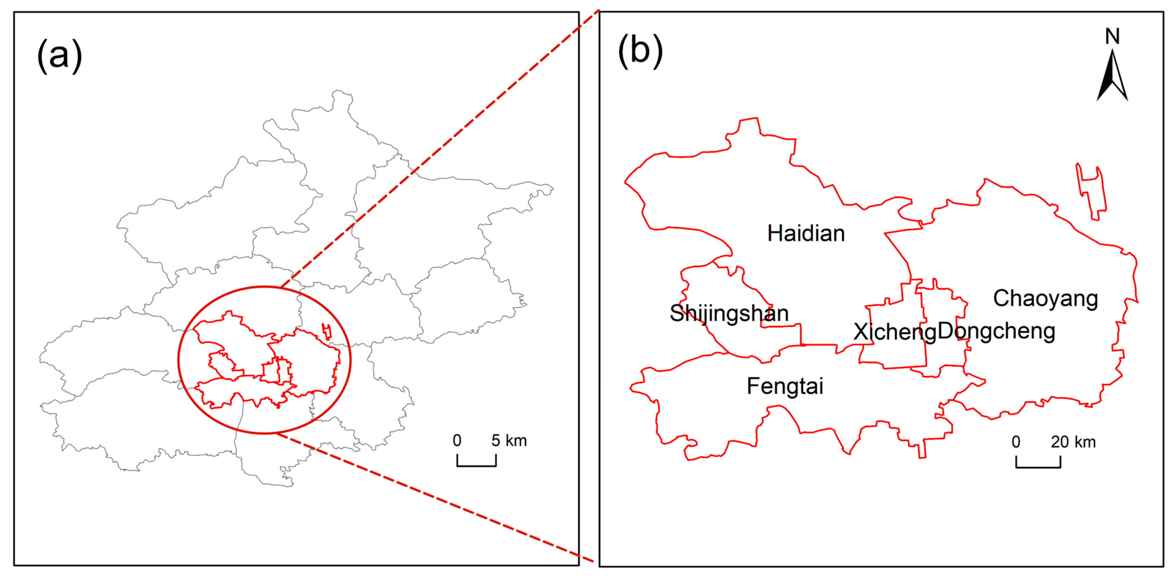
Beijing is the capital of China, its political and cultural center, a world-famous ancient capital, and a modern international city. The main urban area of Beijing (Figure 1) was selected as the research area. The main urban area of Beijing includes Dongcheng District, Xicheng District, Haidian District, Chaoyang District, Fengtai District, and Shijingshan District, with a total area of approximately 1366 km², accounting for 8.3% of the city’s total area. In 2020, the permanent resident population of the main urban area was 10.985 million, accounting for 50.18% of the city’s permanent resident population. The GDP of the main urban area was CNY 2626.08 billion, accounting for 72.76% of the city’s total GDP [22]. Thus, the main urban area is the most concentrated area of population and social and economic activities in Beijing. In addition, in the first quarter of 2023, Beijing’s tourism market showed significant growth compared with the same period in 2022. The number of tourists received was approximately 57.9 million, an increase of about 10%. Tourism revenue was about CNY 105 billion, an increase of about 17%. The prosperous tourist market, highly concentrated business district, and profound cultural heritage provide good conditions for the breeding and development of coffee shops in the main urban area of Beijing [1,7].

2.1.2. Data Collection

This study involved multi-source spatial data (

Table 1. Sources and descriptions of the data used in the study.

Item	Data Sources	Spatial Resolution	Data Description
POI data	Amap API Data Open Interface (https://lbs.amap.com) (accessed on 1 December 2020 and 1 December 2022)	-	Obtained 20 types of POI data in the main urban area
Population density data	LandScan (https://landscan.ornl.gov) (accessed on 1 December 2020 and 1 December 2021)	1 km	Due to the limitation of data sources, the population density data in 2022 were replaced by the 2021 data
Housing price data	Beijing Lianjia Network (https://bj.lianjia.com) (accessed on 1 December 2022)	-	Obtained using crawler technology, the listing price/floor area, and interpolation
Night light data	The Earth Observation Group (https://eogdata.mines.edu/products/vnl/) (accessed on 1 December 2020 and 1 December 2022)	15 arcseconds (Equator ~500 m)	In order to avoid the impact of COVID-19, monthly synthetic products were used, and September images were selected
Road network data	OpenStreetMap (OSM) (https://www.openstreetmap.org) (accessed on 1 December 2020 and 1 December 2022)	-	Five categories—primary, secondary, tertiary, motorway, and trunk—were identified as major urban roads, and the correlation between store distribution and roads was studied
Administrative division data	Beijing Municipal Geographic Information Public Service Platform (https://beijing.tianditu.gov.cn) (accessed on 5 December 2022)	-	Obtained the latest version of the Beijing city and the central city standard base map
Business layout planning data	Beijing Municipal People’s Government (https://www.beijing.gov.cn/) (accessed on 5 December 2022)	-	The special plan for commercial consumption space layout in Beijing (2022–2035) was used to obtain the dynamic consumption circle data of the urban consumption center of the main urban area

), such as basic boundary, social economy, and urban structure data. We processed the data for 2020 and for 2022 separately. Our POI data were based on the first class of POI classifications released by Amap on 10 August 2021, combined with the actual classification requirements; they were processed as follows:

• Eliminate the “place-name and address information” that has no practical significance for prediction.
• Considering the data volume of the “automobile service”, “automobile sales”, and “automobile maintenance” categories, as well as the consistency of their impact on site prediction [23], we combined the points under these three categories into one category, called the “car-related” category.
• Under the category of “catering services”, because the study took the points under the category of “cafe” as the dependent variable, the subcategory of “cafe” was excluded.

After these treatments, we obtained a total of 20 types of POI data (

Table 2. Statistics of the 20 types of POI.

	2020	2022		2020	2022
Catering services	62,639	73,332	Service for life	92,156	89,043
Road-affiliated facilities	1380	91	Event activities	6	13
Famous scenery	5418	6991	Inside plant	11	7
Communal facilities	13,553	11,226	Sports and leisure services	14,512	17,974
Incorporated business	87,651	55,815	Access facilities	37,901	52,412
Shopping services	123,289	115,041	Healthcare services	15,339	17,919
Transportation facilities services	54,676	57,890	Government agencies and social organizations	33,123	31,300
Financial insurance services	12,891	10,017	Accommodation services	18,821	9919
Science, education, and culture services	48,400	38,959	Car-related	13,436	13,087
Motorcycle service	438	576	Commercial residence	33,940	25,332
			Sum	669,580	626,944

). Notably, although the amounts of data for “inside plant” and “event activities” were small, they reflect the distribution of infrastructure such as waiting rooms and terminals as well as the locations of various large-scale activities. These locations have great influence on the public and the city and are the places and destinations where a large number of overseas tourists gather [7,24]. In addition, the waiting properties of waiting rooms, terminals, and other places, as well as the entertainment properties of venues that host large events, have increased the demand for coffee shops; thus, we kept both types of information in the dataset.

2.1.3. Construction of Impact Factors

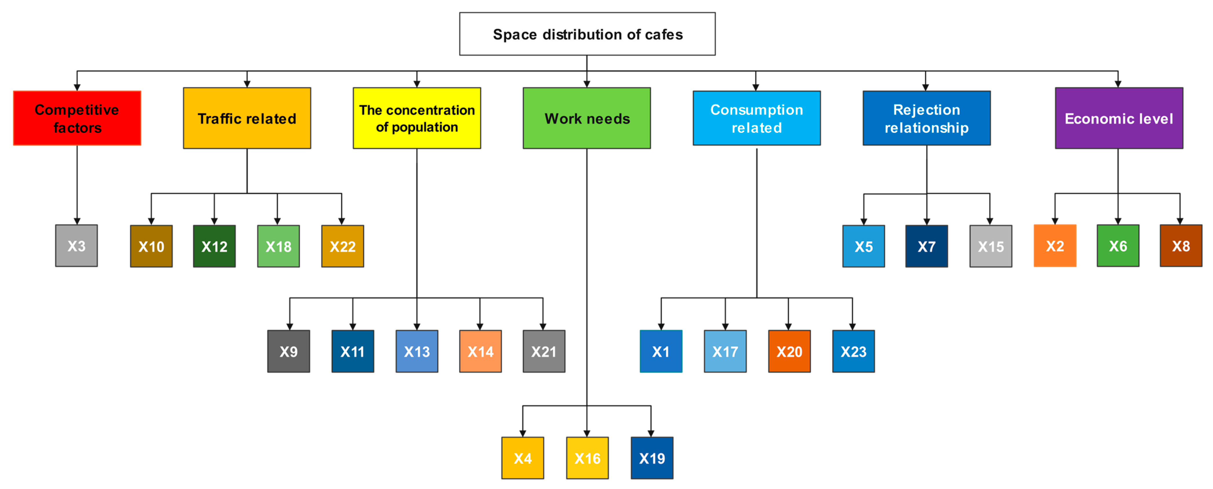
Based on the reference study of Huang Qin by Zha Aiping and Hui-Jia Yee [17,18,25], we preliminarily constructed 23 factors (Figure 2) that may affect the location of cafe stores in 7 ways; the explanations of each factor are shown in

Table 3. The 23 indicators mentioned in Figure 3.

Feature	Name	Handling Method
X1	Sports and leisure services	The result of KDE of POI data
X2	Commercial residence
X3	Catering services
X4	Financial insurance services
X5	Motorcycle service
X7	Car-related
X9	Communal facilities
X10	Transportation facilities services
X11	Science, education, and culture services
X12	Road-affiliated facilities
X13	Famous scenery
X14	Event activities
X15	Healthcare services
X16	Incorporated business
X17	Service for life
X18	Inside plant
X19	Government agencies and social organizations
X20	Shopping services
X22	Access facilities
X23	Accommodation services
X8	Average house prices	The grid data are obtained by Kriging interpolation of discrete housing price points
X6	Night lights	Use raw raster data
X21	Density of population

. Among them, the calculation method of each factor was as follows:

• The kernel densities of the 20 types of POI data and coffee shop distribution data were estimated.
• Raw data on population density and night light were used.
• The average house prices were determined by Kriging interpolation.

In later studies, we will further evaluate the suitability of these indicators, and we will also eliminate the factors with a small influence on site selection, a process called pruning.

It is important to note that the road data covered in Table 1 will be considered separately as factors independently of the 23 influencing factors. Roads are linear elements; therefore, the construction of a multilevel road buffer can filter out a part of the area, reduce the bias generated in the construction model, and may have the potential to improve the accuracy of the location model [26]. Therefore, we discuss the distribution of coffee shops around a road by constructing a multilevel road buffer and study the influence of road buffer construction on the accuracy of the prediction model.

2.1.4. Extraction of Sampling Points

Based on the research of Yu Yue et al. [27] and combined with actual research and accuracy requirements, this study established sampling points on the geometric center of a 500 m grid scale that was within the scope of the main urban area. The values of characteristic factors were extracted from the sampling points. In order to eliminate the dimensional inconsistency of various data, for 2020, we carried out the normalization processing of various characteristic factors and the coffee shop kernel density, as indicated in the following equation:

$$f_j\left(X_i\right)=\frac{X_i-X_{min}}{X_{max}-X_{min}},j=\mathrm{1,2},3,\dots 23$$

(1)

where $j$ is a certain feature, $X_i$ is the value of the sample point feature of $i$, $X_{min}$ is the minimum value of all sample point features, and $X_{max}$ is the maximum value of all sample point features.

2.2. Methods

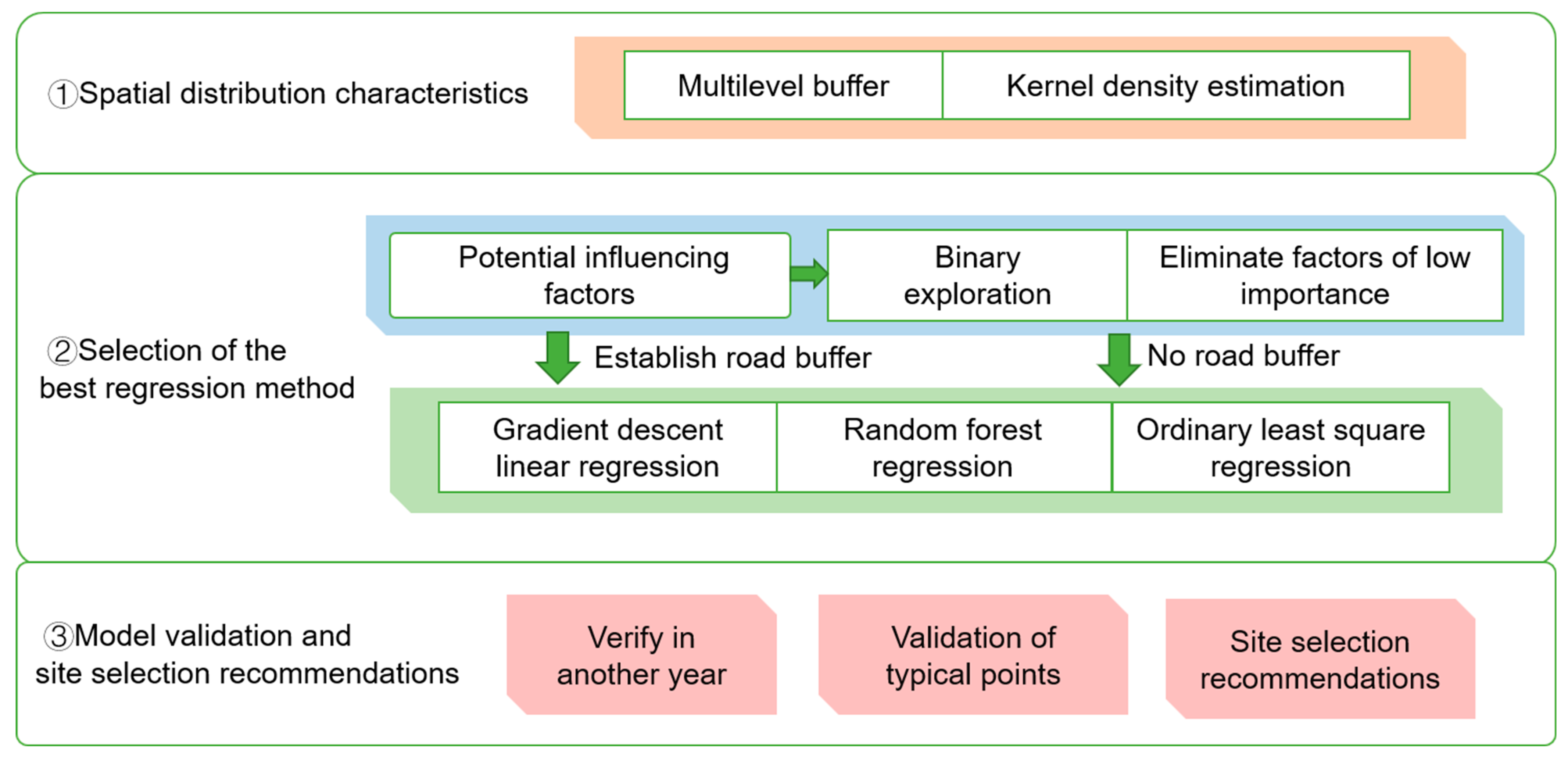
Based on a study of the spatial distribution and agglomeration characteristics of coffee shops, this study compared and selected the three regression methods both before and after considering the road buffer zone, so as to give suggestions on recommended locations for coffee shops. The content of the study (Figure 3) can be summarized as follows:

• Study of the spatial distribution characteristics of coffee shops: with the coffee shop KDE as the base map, an overlay analysis was carried out with the multilevel buffer zone established with Jingshan Park as the center point.
• Comparison of regression methods: on the basis of the construction of characteristic factors and binary classification exploration to determine whether there was a coffee shop in a grid, the regression accuracies of RF, GD, and OLS models were compared and analyzed to select the best model.
• Comparison of regression results considering road constraints: comparative analysis of the regression accuracy of the models before and after the main road buffer zone was established, and comparison and verification of the prediction success rate of the two models.
• Verify the accuracy of the model: by comparing the actual data of two time snapshots with the corresponding prediction results of coffee shop KDE, the probability that the actual trends of coffee shops are consistent with our prediction trend is obtained, thus verifying the accuracy of the prediction model selected in this paper from a practical point of view.
• On the basis of the above steps, the best prediction model is selected, and the evaluation and recommended location of a coffee shop in typical areas are given.

2.2.1. Study of Spatial Distribution Characteristics

Coffee shop data are dotted elements in the main urban area. This study used buffer zone analysis and kernel density analysis to study the spatial distribution characteristics of stores.

KDE is an important statistical analysis method for extracting the distribution characteristics of geospatial facilities. It can represent the agglomeration area of dotted elements in space. If the location is closer to the core element, the kernel density will be greater, indicating a higher aggregation degree of the midpoint in this region [17,28,29]. The formula of the estimation is:

$$f\left(x\right)=\sum _{i=1}^n\frac{1}{r^2}k\left(\frac{x-x_i}{r}\right)$$

(2)

where $f\left(x\right)$ is the kernel density at the point x, n represents the number of elements in the range of distance r from the point x, k is the spatial weight coefficient, and r is the distance decay threshold.

In addition to these parameters, cell size is an important parameter in KDE which directly affects the pixel size of the output kernel density grid image and has a certain impact on the generation of the kernel density image. Some studies have pointed out that the default parameter values determined by the analysis of different cell sizes by some professional GIS products (such as ESRI’s ArcGIS Spatial Analyst) provide practitioners with better image processing quality [30]. Therefore, we adopted the default cell size value in ESRI’s ArcGIS: the value obtained by dividing the width or height (the smaller value) of the factor dataset range by 250.

A buffer zone is a ribbon zone with a certain width that is used to identify the influence of a spatial object on its surrounding features [31]. For a given object, its buffer can be defined as:

$$P=\left\{x\right||d\left(x,A\right)\le r\}$$

(3)

where d refers to the distance between point x and point A in space, according to different application fields, with the expression of the distance also being different; r is the neighborhood radius or buffer’s established conditions. There are three common patterns in buffer analysis: the point, line, and surface. By establishing a buffer zone, the influence ranges of geographical elements can be expressed. In this paper, we set up a multilevel buffer zone centered on Jingshan Park to study the spatial distribution characteristics of coffee shops and took the constraints of main roads in the city as a buffer zone to screen out some areas for better site selection.

2.2.2. Prediction Method

(1)

Random Forest Algorithm

RF, proposed by Leo Breiman [32] in 2001, is a bagged integration algorithm based on machine learning theory. It is widely used to solve classification, regression, and other data mining problems, and it can also evaluate the importance of classification and predictive variables [33]. Research by Hui-Jia Yee et al. [18] has showed that RF models have high accuracy among many machine learning models used for location problems. Therefore, we choose this method to be compared with the other two regression methods.

The basic process of establishing the RF model is that the training samples are randomly selected to establish multiple decision trees, which constitute a base evaluation sequence $\{h_1\left(X\right),h_2\left(X\right),h_3\left(X\right),\dots ,h_k\left(X\right)\}$, and the order or average of the prediction results of each base evaluation sequence determines the prediction results of the unknown sample.

$$H\left(x\right)=\mathit{arg}{max}_y\sum _{i=1}^{k}I(h_i\left(X\right)=Y)$$

(4)

where $H\left(x\right)$ represents the final result of the model, $I$ is the schematic function, $h_i$ is the base evaluator, and $Y$ is the target variable. When Y is a classification variable, the model is used to solve the classification problem. When Y is a continuous variable, the model is used to solve the regression problem [34].

RF can evaluate the impact of displacement importance. The core idea is to judge the importance of features by comparing the prediction accuracy of the model before and after adding noise. If the model prediction accuracy is greatly reduced, the feature is important.

RF cannot obtain certain equations as traditional models do, and it usually uses the data to evaluate the model [35,36]. Usually, the established model is applied to the training and test data, and the model evaluation results are obtained. In this study, we uniformly used 70% of the data for training and the remaining 30% of the samples for testing.

In RF classification problems, the error is the error rate of the classification, and the model performance is often evaluated based on a confusion matrix. In this study, we selected $Recall$, $Precision$, and $F1$ to evaluate the model performance with the following formulae:

$$Recall=\frac{TP}{TP+FN}$$

(5)

$$Precision=\frac{TP}{TP+FP}$$

(6)

$$F1=\frac{2\times Precision\times Recall}{Precision+Recall}$$

(7)

where $TP$ is the number of true classes, $FP$ is the number of false-positive classes, and $FN$ is the number of false-negative classes. The $F1$ score is the harmonic average of the precision and recall, and the larger the three indicators, the better the classifier is.

(2)

Gradient descent algorithm

GD is the solution for the minimum [37] in the direction of a negative gradient. The basic idea is to use the GD algorithm to solve the cost function so that the cost function loses the minimum value. Because this method can go through several iterations and has the smallest gap between the estimated value and the target value, it can be used to solve the optimization problem of model parameters and is widely used [38]. In this paper, the GD model is used to optimize the OLS parameters, and the accuracy of the results is compared with the traditional OLS regression method. Suppose that the linear regression function is:

$$h_{\theta }\left(x\right)=\sum _{i=0}^n{\theta }_i{x}_i={\theta }^{T}x$$

(8)

and $x_0=1$.

$$J\left(\theta \right)=\frac{1}{2m}\sum _{i=1}^m{\left(h_{\theta }\left(x^{\left(i\right)}\right)-y^{\left(i\right)}\right)}^2$$

(9)

where $x$ is a feature, the corresponding $\theta$ is the regression coefficient of this feature, n is the number of features, $m$ is the number of samples, $h_{\theta }\left(x\right)$ is the predicted value, $y^{\left(i\right)}$ is the actual value, and $J\left(\theta \right)$ is the cost function. For the $\theta$ of j, the loss function gradient is [39]:

$$J\left(\theta \right)=\frac{1}{m}\sum _{i=1}^m\left[\right(h_{\theta }\left(x^{\left(i\right)}\right)-y^{\left(i\right)}\left){x_j}^{\left(i\right)}\right]$$

(10)

To minimize the cost function loss value, iteration can be performed using the following methods:

$${\theta }_j≔{\theta }_j-\alpha \frac{\partial }{{\partial \theta }_j}J\left(\theta \right)$$

(11)

where $\alpha$ is the learning rate used to control the step size of the GD. As the number of iterations increases, the parameter reaches a stable point and no longer changes, yielding the determined regression coefficient.

(3)

Ordinary least squares method

OLS is a traditional linear regression method which is based on minimizing the model based on the mean square error. Its main aim is to minimize the sum of squares of the difference between the predicted value and the actual value by solving a set of unknowns [36]. As a classical and stable linear regression model, we use this model as a benchmark to compare with two other machine learning regression models. Suppose that the linear regression function is:

$$h_{\theta }\left(x\right)=X\theta$$

(12)

where $h_{\theta }\left(x\right)$ is the $m\times 1$ dimension vector, $\theta$ is the $n\times 1$ dimension vector, $X$ is the $m\times n$ matrix, m is the number of samples, and n represents the number of features. The loss function of $\theta$ is defined as:

$$J\left(\theta \right)=\frac{1}{2}{(X\theta -Y)}^T(X\theta -Y)$$

(13)

where $Y$ is the output vector of the sample, and the dimension is $m\times 1$. According to the principle of least squares, this means that:

$$\frac{\partial }{{\partial \theta }_j}J\left(\theta \right)=0$$

(14)

After finishing, we find that:

$$\theta ={{(X}^{T}X)}^{-1}{X}^{T}Y$$

(15)

(4)

Construction of road buffer zone

In cities, most of the store facilities are distributed along the streets [26], and human activities are also constrained by the roads, while the traditional analysis method is based on the whole region, which has some limitations. For example, the traditional analysis method generally adopts the globally consistent parameter model for analysis but ignores the spatial non-stationarity of the influencing factors when applied to the analysis of commercial facility vitality [40]. Therefore, our study considers the comparison of multivariate regression models taking into account road constraints. Based on OSM data, this paper establishes a multilevel buffer zone for the key roads in the main urban area of Beijing by setting appropriate distance intervals through analysis.

(5)

Precision evaluation of the model

For the regression models of RF and the GD, we used the mean squared error (MSE), root-mean-square error (RMSE), mean absolute error (MAE), and R² indicators to evaluate the models [35]. The calculation method is as follows:

$$MSE=\frac{1}{m}{\sum _{i=1}^m(y_i-\widehat{y_i})}^2$$

(16)

$$RMSE=\sqrt{MSE}$$

(17)

$$MAE=\frac{1}{m}\sum _{i=1}^m|y_i-\widehat{y_i}|$$

(18)

$$R^2=1-\frac{{{\sum }_{i=1}^m(y_i-\widehat{y_i})}^2}{{{\sum }_{i=1}^m(\overline{y_i}-y_i)}^2}$$

(19)

where $y_i$ is the true value of the table sample, $\widehat{y_i}$ represents the predicted value of the sample, and $\overline{y_i}$ represents the mean value of the samples. $RMSE$ is the square-root value of the MSE. The MAE is the mean value of the absolute error, which can reflect the actual situation of the predicted error. The smaller the values of the above three indicators, the higher the accuracy of the model.$R^2$ is the coefficient of determination, and the closer the value is to 1, the higher the model accuracy is.

For the regression model established via the OLS method, we analyzed the linear relationship by analyzing the value of $F$ and the value of $P$, analyzed the model fit using the R² value, explored the influence of the independent variable on the dependent variable using the significance of the P-value, and studied the influence of the independent variable on the dependent variable with the value of the regression coefficient, B.

3. Results

3.1. Spatial Distribution Characteristics

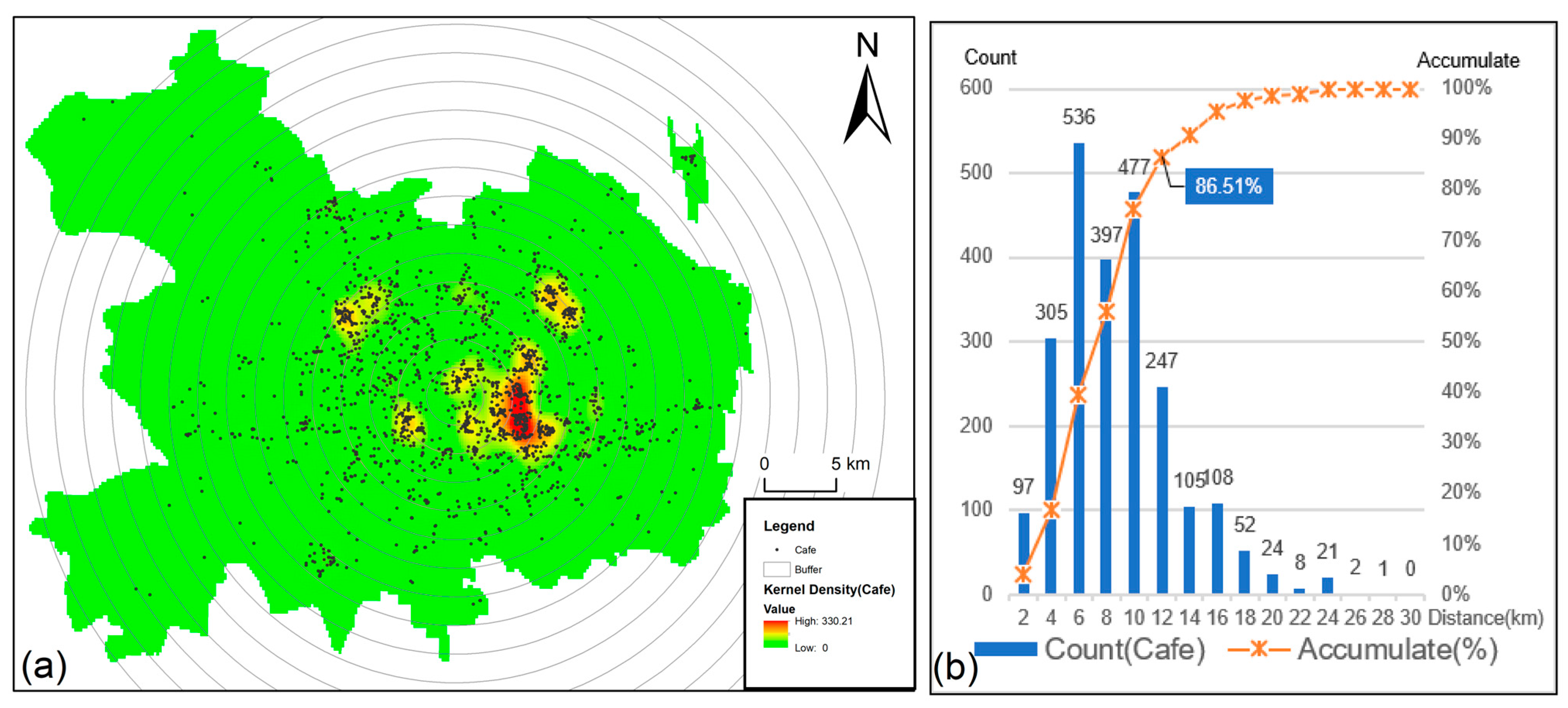
In order to understand the distribution characteristics of coffee shops in the main urban area of Beijing, a multilevel buffer zone was established every 2 km in an outward direction, with Jingshan Park being the center of Beijing. We conducted a statistical analysis of the number of coffee shops in each buffer zone (Figure 4b). From the cumulative number of stores at different distances from the central point (Figure 4b), it was found that more than 85% of the coffee shops in the main urban area of Beijing are concentrated in an area within 12 km of the central point. Because a single central buffer cannot represent the true aggregation range [12], we overlayed the KDE (Figure 4a) results with the multilevel buffer we had established. Through the observation of kernel density interpolation images, we found that the coffee shop distribution features had obvious agglomeration effects, and multiple regions with high kernel density values were generated within 2–10 km of the central point. The distribution of high values was consistent with the conclusion of the buffer analysis.

3.2. Binary Classification Exploration and Regression Method Selection

3.2.1. Exploratory Study Based on RF Classification

After the extraction of sampling points, in order to explore the feasibility of the location selection method in this paper, we first carried out binary classification of the sampling data to determine whether there was a coffee shop in a grid. We established a spatial connection between a base set of cafe points and a 500-square-meter grid and divided the sampling points into two categories based on the number of coffee shops contained in each grid. We set the value of 4586 grids with no coffee shop to 0 and the value of 922 grids with at least one coffee shop to 1. Then, the 23 influencing factors constructed above were taken as independent variables, and the binarized coffee shop data were taken as dependent variables for classification by the RF algorithm. In order to reduce the accidental error of the experiment, after 50 rounds of experiments, the arithmetic average of the numbers of various types in the results of RF classification was taken, as shown in

Table 4. Accuracy evaluation of binary RF classification.

	Sampling Number	Recall	Precision	F1
Training set	3854	0.924	0.922	0.921
Test set	1653	0.895	0.887	0.888

.

Table 4 shows that the average test accuracy rate was 88.7%, and the recall rate was 89.5%, both of which reached a high level, and the average F1 score was 0.888, which reflected that the precision and recall rate also reached a high level after the average reconciliation. Therefore, we found that the sampled data achieved high performance when they were used for binary classification of the presence and absence of coffee shops; thus, they could be used for multivariate regression and predictions of coffee shop kernel density based on the sampled data.

Therefore, we conducted regression based on the RF algorithm for the sampled data, taking the coffee shop KDE as the dependent variable and the other 23 possible influencing factors as independent variables for regression. To improve the stability of the model, after 50 rounds of experiments, the experimental average results are shown in

Table 5. RF model accuracy before pruning (2020).

	MSE	RMSE	MAE	R2
Before pruning	0.001	0.029	0.015	0.907

and Figure 5a.

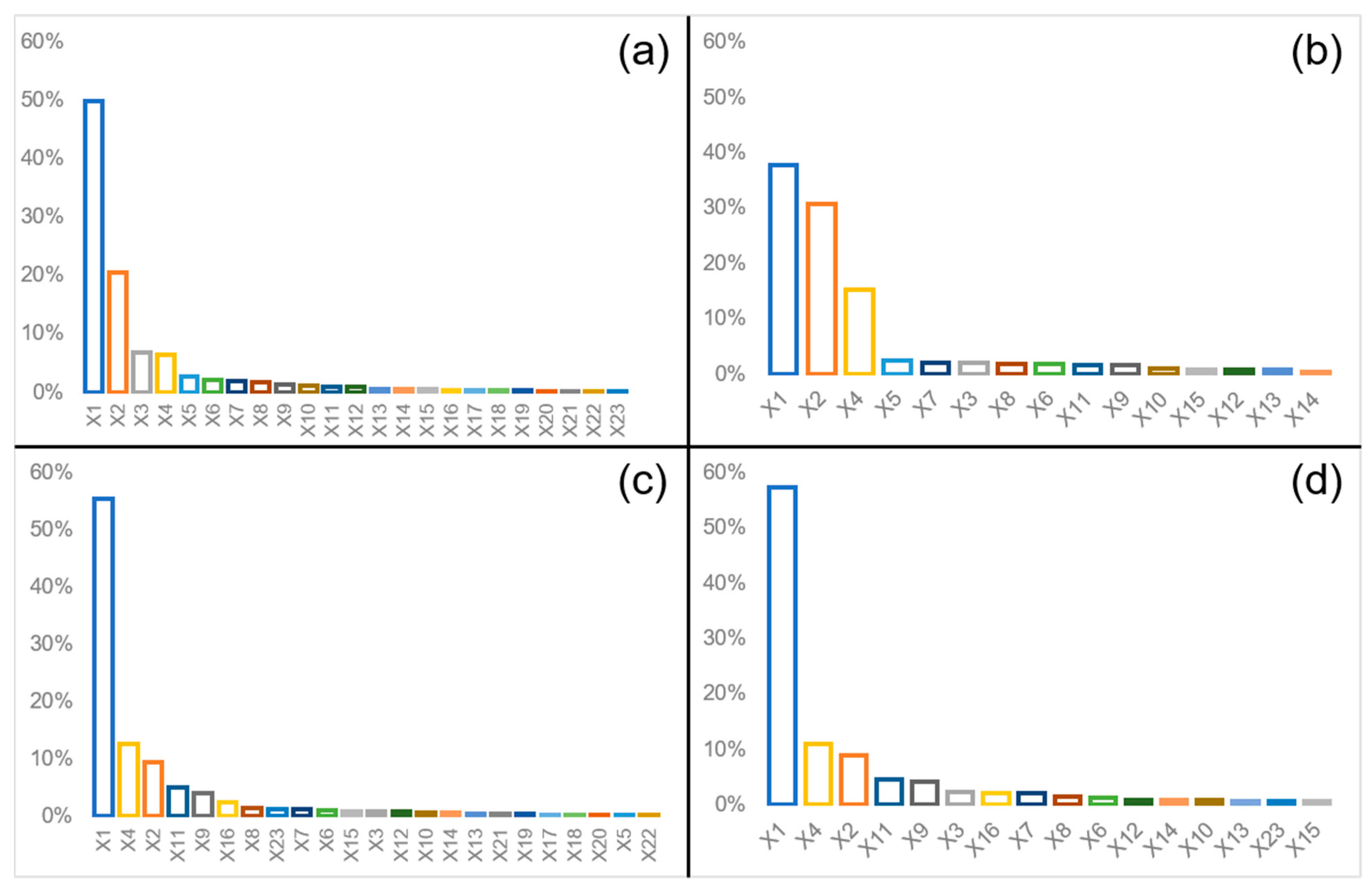
Table 5 shows that the average MSE, RMSE, and MAE were 0.001, 0.029, and 0.015, respectively, i.e., small values, which shows that the expected difference between the predicted value and the actual value was very small; the average R² was 0.907, which is close to 1. The validation results showed that the sampled data also achieved high accuracy when used for multivariate regression. Regarding the characteristic importance of influencing factors, sports and leisure services (X1), commercial residences (X2), catering services (X3), and financial insurance services (X4) were the main factors that had a significant impact on the spatial distribution of coffee shops [3]. We found that X15 to X23 were eight factors which had low importance, and the average of the low-influence factors was relatively higher. In order to simplify the model and improve the applicability and accuracy and taking into account the actual research and precision control needs, in the subsequent experiment we eliminated eight influencing factors whose average feature importance was less than 0.5%.

3.2.2. Comparison of Multivariate Regression Methods

After eliminating the influencing factors where the average importance of the characteristic was too small, 15 influencing factors were taken as the independent variables, and the coffee shop KDE was taken as the dependent variable. RF model regression, linear regression based on the GD method, and OLS regression were selected to predict the kernel density of the coffee shops. In order to improve the stability of the model, after 50 rounds of experiments, the experimental average results were obtained, as shown in

Table 6. The accuracy of the RF, GD method, and OLS regression models.

		MSE	RMSE	MAE	R2
Before buffer analysis	RF	0.001	0.029	0.015	0.915
	GD	0.001	0.037	0.021	0.873
	OLS	-	-	-	0.859

and Figure 5b.

The results show that the MSE, RMSE, and MAE values of the two machine learning regression methods based on RF and the GD method were small, which reflects the expected difference between the predicted value and the actual value. The significance level, P, of the most influential factors in the OLS regression was validated. This indicates that the effect of excluding low-importance features from the RF model is ideal. From the perspective of R², RF > GD > OLS. In general, the three regression methods had high accuracy and could predict the kernel density of coffee shops; the RF model achieved the best prediction effect.

3.2.3. Comparison of Multivariate Regression Accuracy of the Main Road Network Constraints

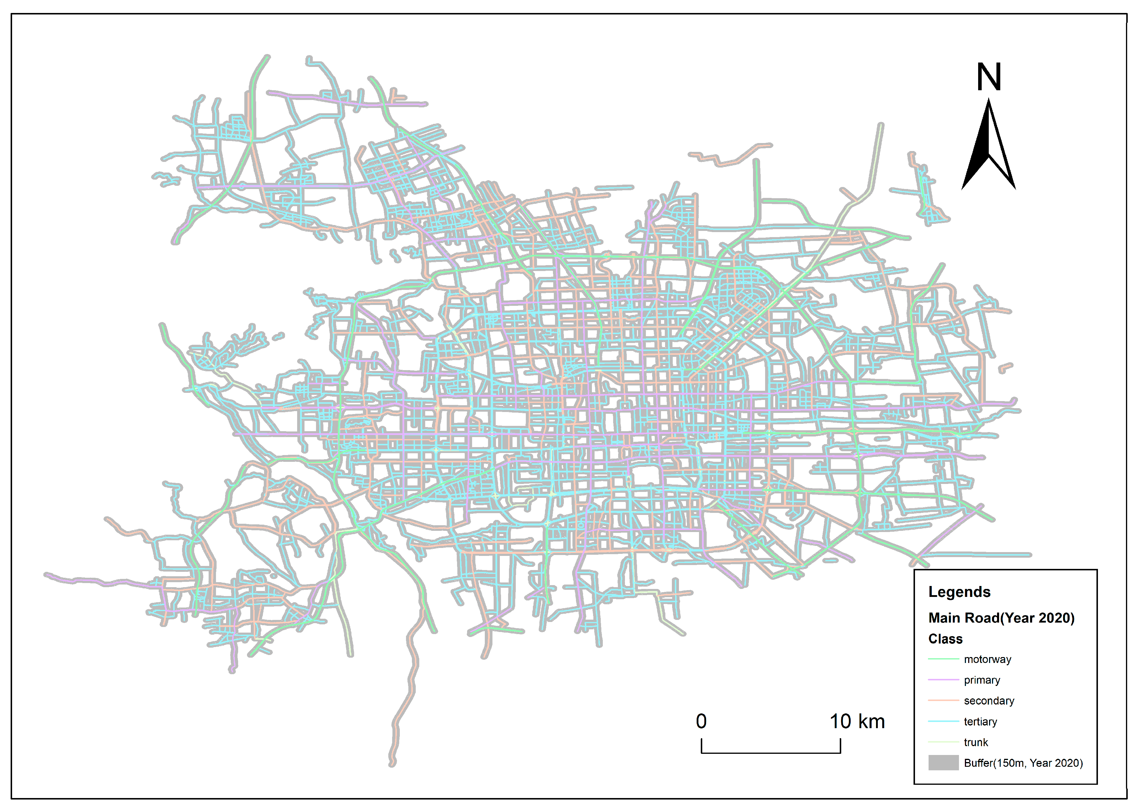
The results of constructing a multilevel road buffer are shown in

Table 7. Multilevel buffer with 50 m radius based on the main road.

Distance/m	(0,50)	(50,100)	(100,150)	(150,200)	(200,+∞)
Counts	893	737	302	147	303
Cumulative ratio	37.49	68.43	81.11	87.28	100.00

and Figure 6 We found that, similar to most commercial facilities, coffee shops were mainly distributed along roads. The zoning statistics show that about 81.1% of the coffee shops were distributed in the buffer zone 150 m away from the main road network. Therefore, we selected sampling points within the buffer zone 150 m from the main road for further regression analysis. Similarly, comparative analysis of the three regression methods was still used after establishing the road buffer zone. In order to improve the stability of the model, after 50 rounds of experiments, the average experimental results were obtained, as shown in

Table 8. The accuracy of the RF, GD method, and OLS regression models after buffer analysis.

		MSE	RMSE	MAE	R2
After buffer analysis	RF	0.001	0.035	0.021	0.929
	GD	0.002	0.041	0.027	0.893
	OLS	-	-	-	0.872

.

The experimental results showed that after the regression prediction of buffer processing, the accuracy of the three models changed as follows: for machine learning regression based on RF and the GD method, the accuracy of RMSE and MAE decreased, while the R² values of both datasets increased from 0.915 and 0.873 to 0.929 and 0.893, respectively. For the OLS method, R² also exhibited a relatively high increase. In general, after buffer processing, the R² ranking of the three models did not change, and the regression effect of machine learning based on RF was the best. However, the accuracy of various regression analyses on the sampled data was improved to a certain extent, which is in line with the above speculation.

Thus far, we have compared the three regression methods under the conditions of buffer analysis and non-buffer analysis and achieved comprehensive analysis results of the model prediction accuracy. The analysis found that the RF method outperformed the GD and OLS methods in the buffer analysis and non-buffer analysis. Between the RF model and the OLS model, the prediction accuracy of RF also outperformed OLS, which indicates that the site selection prediction in this paper may be more biased toward nonlinear influence [41], which is consistent with the discussion of Michael Nwogugu et al. [13]. Within the context of observing the similar distributions of various regression features, we decided to choose the RF model with better generalization ability and higher prediction accuracy under the two analysis conditions as the basic method of our site selection model. However, whether buffer processing is carried out or not has little impact on the prediction accuracy, and whether buffer processing is to be carried out or not needs further practical performance verification.

3.3. Practical Verification

After selecting the RF model as the best regression prediction model, we verified the utility of the model before and after establishing the buffer zone in this section. First, we treated the same data in the study area in 2022 using the same method and built an RF site prediction model to compare the similarities and differences between the model and the data from 2020. Secondly, we combined the hierarchical layout plan of the commercial consumption space in the central urban area of Beijing and used the model to evaluate the location suitability of coffee shops in each consumption space in the region, verifying the practicability of the model through the changing trends in the actual kernel density of stores in 2022 compared with 2020.

3.3.1. Construction of the Site Selection Model in 2022

(1)

Comparison of exploratory studies based on RF

After the RF regression modeling of possible factors, the model accuracy (

Table 9. Regression accuracy of the RF model in 2022.

	MSE	RMSE	MAE	R2
Before pruning	0.001	0.03	0.016	0.907
After pruning without buffer	0.001	0.028	0.015	0.920
After creating the buffer zone	0.001	0.035	0.02	0.921

) in 2022 was compared with the model accuracy in 2020 (Table 5, Table 6, and Table 8). By comparing the indicators in the test set, we found that the prediction accuracy of MSE and R² was consistent in the two years, with R² being as high as 0.907; the RMSE and MAE in 2022 were only 0.01 lower compared with 2020. By comparing the rankings of feature importance in the two years (Figure 5a,c), we found a strong consistency in trait importance across the two years, with sports and leisure services (X1), financial insurance services (X4), and commercial residence (X2) being among the top five in both years; density of population (X21), access facilities (X22), shopping services (X20), government agencies and social organizations (X19), service for life (X17), and inside plant (X18) were all less than 0.5%. In 2022, we also eliminated eight influencing factors with an average feature importance of less than 0.5%: X5, X13, and X17–X22. After excluding factors with an average feature importance of less than 0.5% in both years of regression analysis, the importance ranking of each influencing factor is shown in Figure 5b,d. Accuracy evaluations are shown in Table 6 and Table 9.

In conclusion, in the two-year RF exploratory study, the RF model maintained high accuracy, and the selected feature factors maintained high stability.

(2)

Precision of the RF model before and after establishment of buffer

Due to the high accuracy of the RF model in 2020, we compared the prediction accuracy of the RF model with the data from 2022. Similarly, we reduced the accuracy of the road buffer zone and compared the model before and after the establishment of the road buffer zone (Table 8 and Table 9). The results show that the accuracy in 2020 is consistent with the accuracy in 2022, and R² is closer to 1 for RF regression with buffer establishment; for the RF model without a buffer, the RMSE and MAE are closer to 0. In the two years of processing, the quality of the accuracy evaluation index remained consistent before and after adding the buffer, which verified the stability of the model prediction for different years, which meant that adding the road buffer did not cause too much of an impact on the accuracy of the location selection.

3.3.2. Forecast Results of Commercial Consumption Space

As the core framework of constructing an urban consumption space network, the commercial consumption agglomeration area plays a vital role in economic development. Taking Beijing in 2021 as an example, the final consumption rate of the commercial consumption agglomeration area was about 60%, which contributed significantly to urban economic growth. According to the data, the commercial consumption agglomeration area is the core factor influencing residents’ leisure and entertainment, as well as being the main site for coffee shops [5,7,12]. In light of the characteristics of a high consumption rate and high flow of people in commercial consumption gathering areas, we selected the urban consumption center and regional dynamic consumption circle included in the main urban area of Beijing for site selection prediction and verification in order to provide suggestions for coffee store locations and the sustainable development of the spatial pattern of commercial consumption.

(1)

The distribution relationship between the commercial consumption agglomeration area and coffee shops

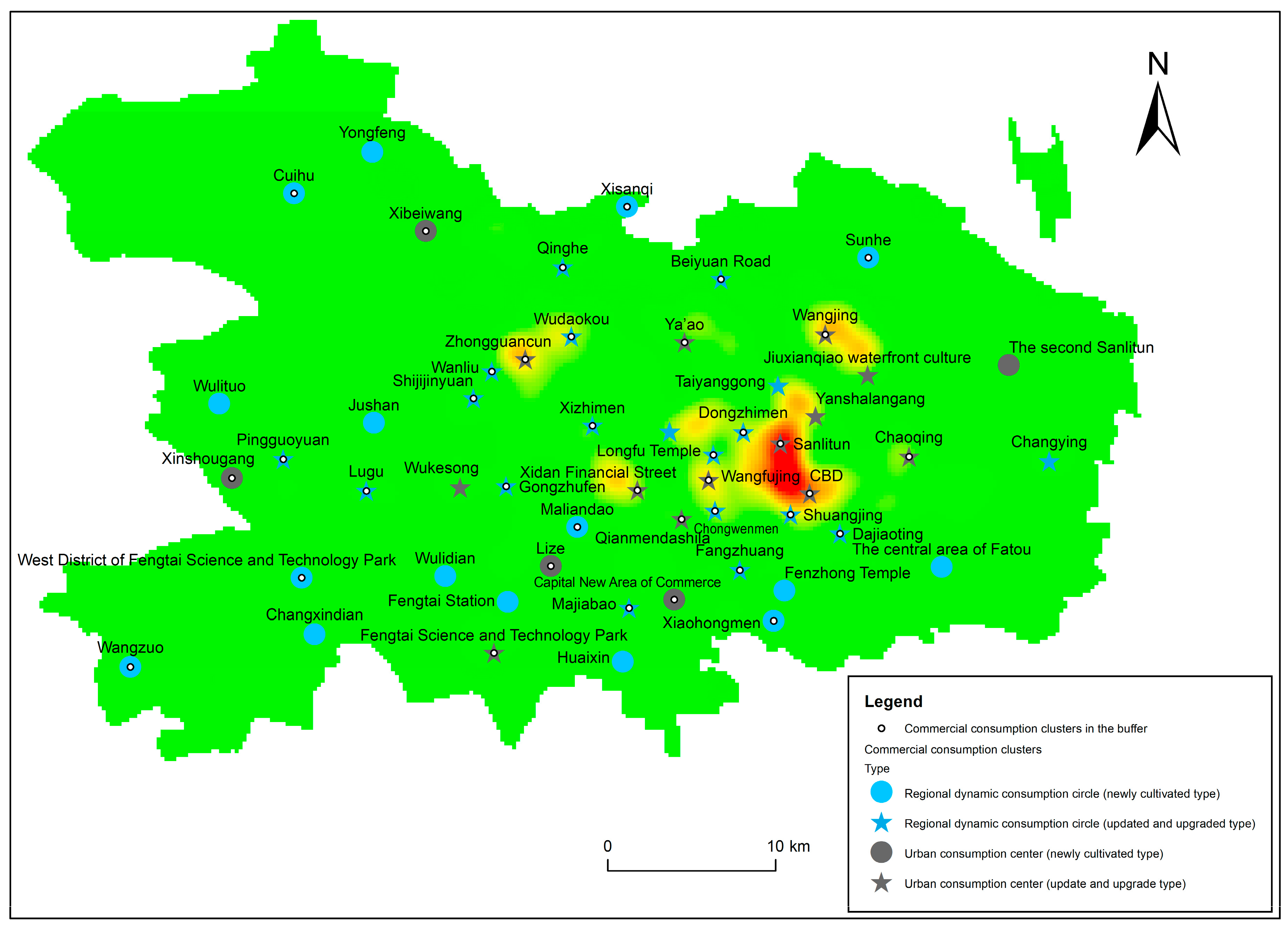
The Special Plan of Beijing Commercial Consumption (2022–2035) divides these commercial consumption cluster areas into newly cultivated and updated types. We analyzed the kernel density of coffee shops and urban consumption center elements (Figure 7).

Table 10. Average kernel density of all types of commercial consumption agglomeration areas.

	Average Kernel Density
Main urban area	16.35
Commercial consumption clusters	49.21
Commercial consumption clusters (updated and upgraded type)	78.27
Commercial consumption clusters (newly cultivated type)	4.92

shows the average kernel density of commercial consumption clusters.

The results in Table 10 show that the average kernel density of coffee shops in all commercial consumption agglomeration areas was 49.21, and the average core density of coffee shops in the updated and upgraded commercial consumption agglomeration areas even reached 78.27, which was much higher than the average kernel density of coffee shops in the main urban area: 16.35. In addition, there were 1835 coffee shops in the buffer zone of the commercial cluster area, accounting for 77.04% of all coffee shops in the main city. Therefore, it can be considered that the commercial consumption agglomeration area is closely related to the kernel density of Beijing coffee shops, as shown by the fact that the updated and improved commercial consumption agglomeration area highly coincided with the high-value kernel density of coffee shops, and the commercial consumption cluster area had a strong agglomeration effect on coffee shops.

(2)

Predicting the success of commercial consumption clusters

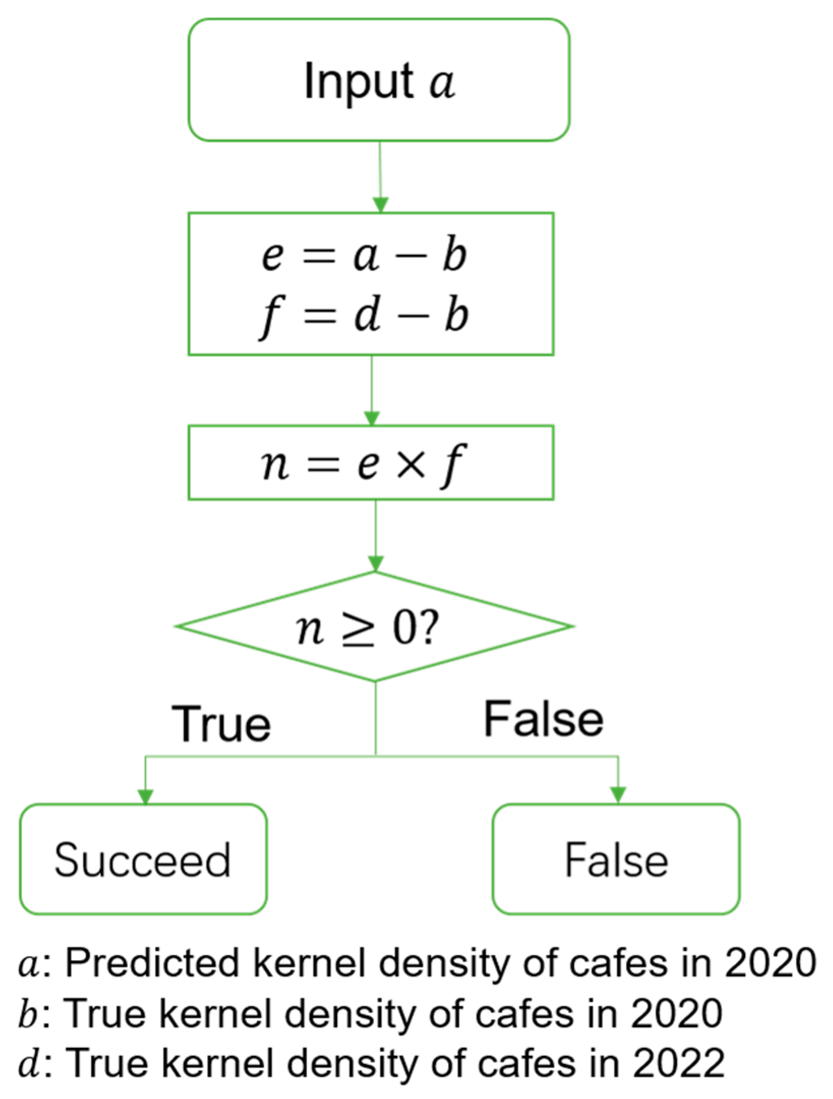
Therefore, we believe that the commercial consumption cluster is a typical area suitable for the location of coffee shops and can be used to verify the practicality of the model. Here, we used the image difference operation method in the digital image processing field to monitor the change information [42,43] in order to show the growth trend of coffee stores. As shown in Figure 8, by subtracting the predicted kernel density value in 2020 from the actual kernel density value in 2020 (e), it could be determined whether the site selection was recommended or not. If the difference was greater than 0, site selection was recommended. If the difference was less than or equal to 0, site selection was not recommended. By subtracting the actual kernel density value of 2020 from that of 2022, the actual change trend for coffee shops is represented [29]. If the recommendation results agreed with the actual trend (e × f ≥ 0), the prediction was successful; otherwise, the prediction failed.

Notably, in order to examine the impact of market saturation factors on location selection results, we focused on the actual changing trends of coffee shops in 53 commercial consumption clusters from 2020 to 2022. The results showed that the kernel density of 38 coffee shops increased positively, accounting for 71.7% of all commercial consumption clusters. This indicates that the coffee shop market in the commercial consumption clusters of the main urban area of Beijing had not reached saturation as a whole and will not considerably impact the site selection results.

The prediction results are as follows. When the main road buffer zone had not been established, there were 53 commercial consumption cluster areas, with 39 cases of the RF model predicting successfully and 14 cases of it failing; in addition, the actual prediction success rate was shown to be 73.58%. After the establishment of the road buffer zone, we eliminated 16 commercial consumption cluster areas that were not in the road buffer zone and predicted 37 commercial consumption cluster areas. The RF model successfully predicted 27 cases and failed in 10 cases, and the actual prediction success rate was 72.97%. After eliminating the low-probability distribution area for the coffee shops, the model still maintained a comparable prediction success ratel; therefore, we recommend using the model with the road buffer zone.

3.3.3. Site Selection Advice

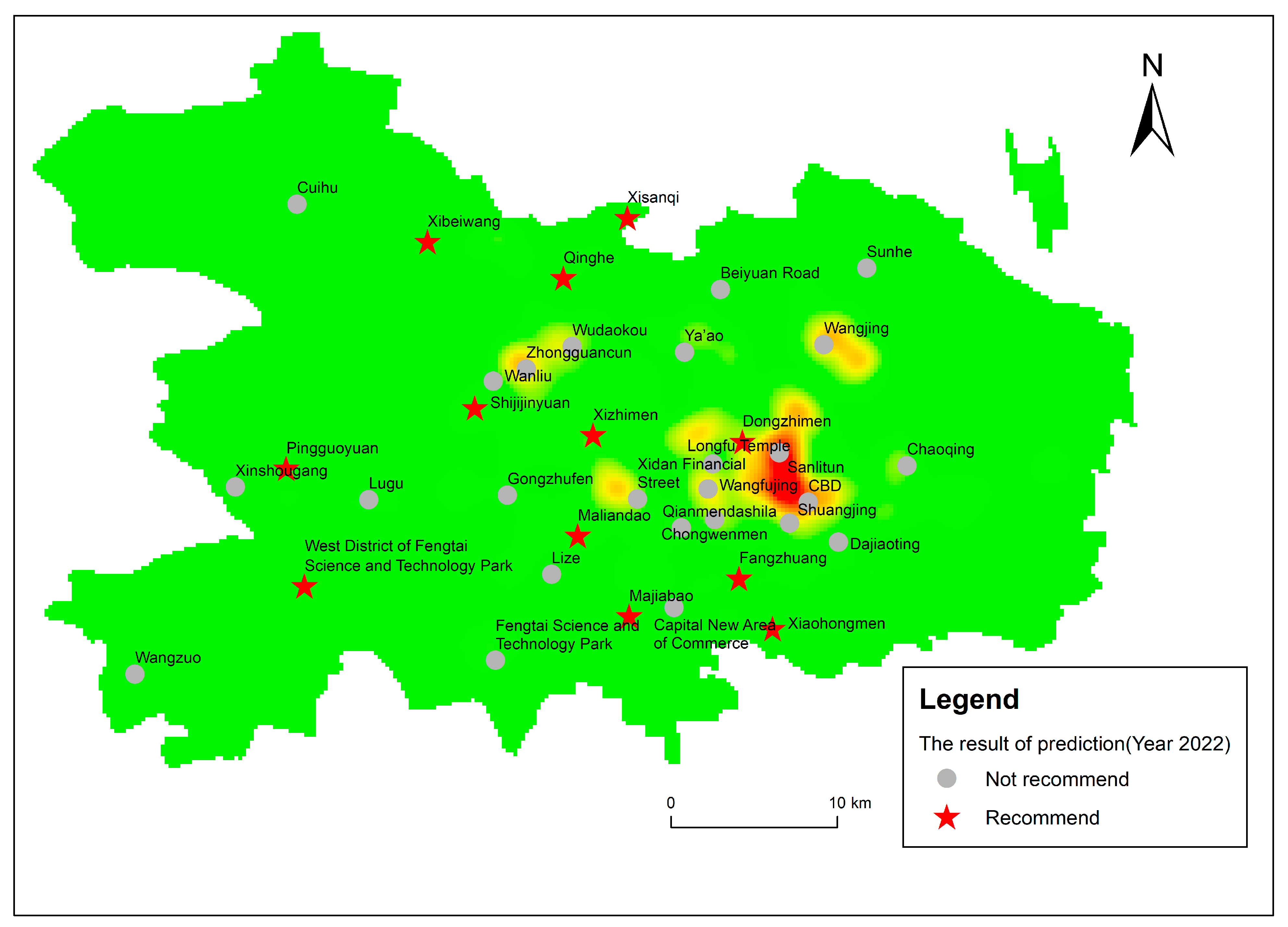
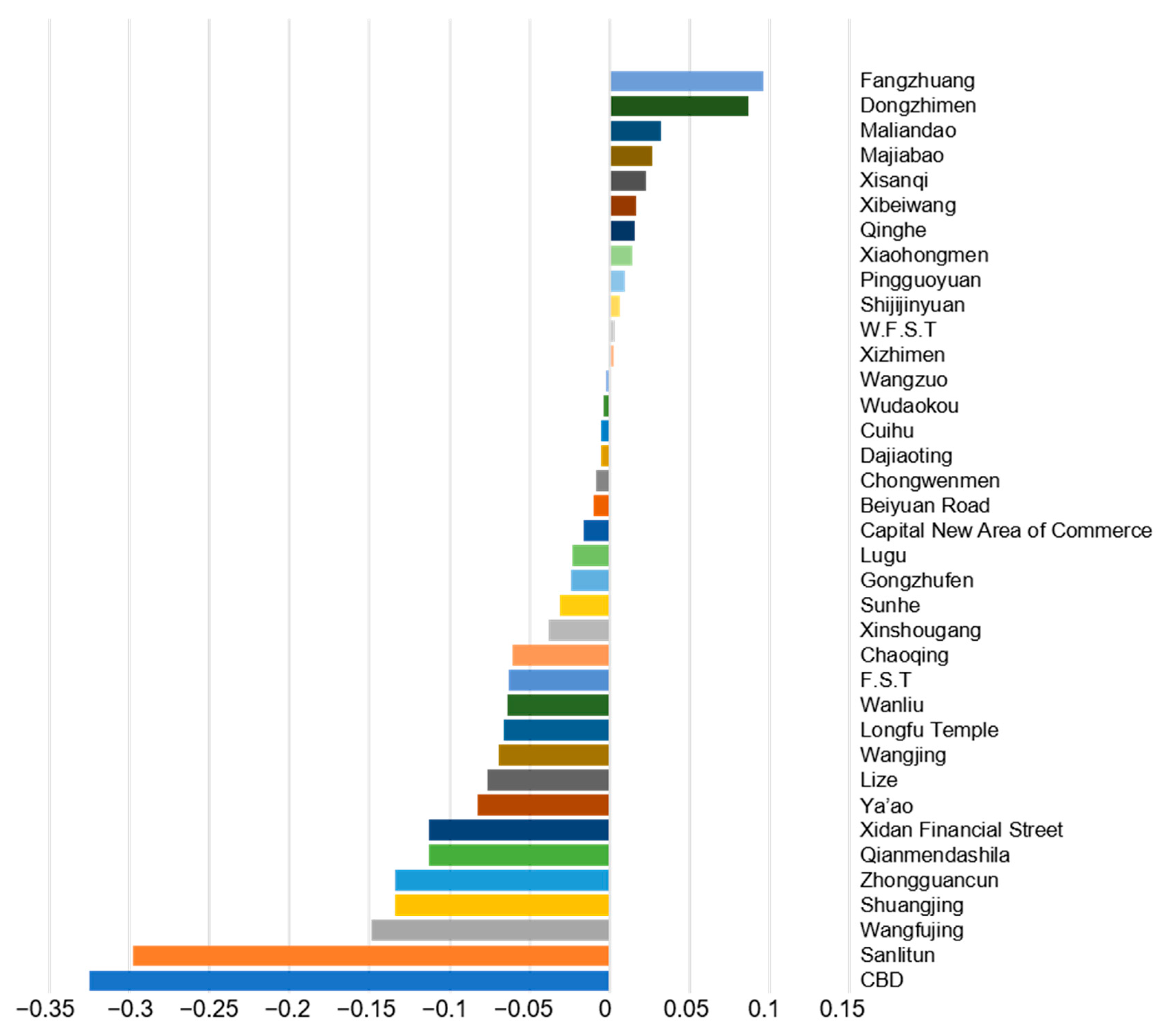
The verification results of the success rate in the previous section show that the model with the road buffer zone is suitable for predicting the locations of coffee shops. Therefore, we used this model and the POI data obtained in 2022 to predict the site selection suitability of coffee shops in the commercial consumption agglomeration areas in Beijing, providing us with site selection suitability suggestions (Figure 9 and Figure 10).

The difference between the predicted value in 2022 and the actual value in 2022 reflects the degree of suitability for opening a coffee shop. The larger the value, the stronger the suitability and the higher the recommendation degree. The recommendation degree of each commercial consumption cluster is shown in Figure 10. We suggest that the top 10 business districts are Fangzhuang, Dongzhimen, Malandao, Majiabao, Xisanqi, Xibeiwang, Qinghe, Xiaohongmen, Pingguoyuan, and Shijijinyuan. Among them, there are nine regional dynamic consumption circles, one urban consumption center, six renewal and upgrading commercial agglomeration areas, and four newly cultivated commercial agglomeration areas. Established commercial and consumer centers such as CBD, Sanlitun, and Wangfujing are the least recommended, reflecting the intense pressure on coffee shops in these areas.

4. Discussion

4.1. Effect of Feature Factors

In the process of conducting multivariate regressions, we tried to analyze and explain the influence of features on coffee shops according to the distribution of feature importance and the size of the regression coefficient. The feature importance of RF (Figure 5b,d) and the GD regression coefficient (

Table 11. Regression coefficient and accuracy evaluation obtained by using GD linear regression.

		2020	2022
Influencing factors	Incorporated business	-	0.184
	Accommodation services	-	0.065
	Financial insurance services	0.589	0.534
	Sports and leisure services	0.441	0.466
	Catering services	0.207	0.081
	Communal facilities	0.143	0.152
	Commercial residence	0.110	0.072
	Science, education, and culture services	0.099	−0.008
	Famous scenery	0.056	0.060
	Average house prices	0.023	0.038
	Event activities	0.017	−0.049
	Night lights	−0.005	0.055
	Road-affiliated facilities	−0.012	0.010
	Car-related	−0.023	−0.053
	Motorcycle service	−0.034	-
	Transportation facilities services	−0.151	−0.226
	Healthcare services	−0.183	−0.146
Accuracy evaluation	MSE	0.001	0.001
	RMSE	0.037	0.037
	MAE	0.021	0.022
	R2	0.873	0.879

) in 2020 and 2022 were comprehensively considered.

We found that sports and leisure services (X1), financial insurance services (X4), and commercial residences (X2) had large positive effects on the distribution of coffee shops, indicating that these categories have a strong agglomeration effect on coffee shops. Nowadays, the definition of a cafe mostly focuses on “leisure and entertainment”, “providing a leisure and comfortable environment”, etc. [44]. Cafes not only exist to provide people with various coffee drinks; they also represent a lifestyle and life concept [45]. This explains the effect of sports and leisure facilities on the distribution of coffee shops. Commercial residential areas include standard and high-end residential areas, and most of the financial and insurance services are office areas, which represent a large number of places where white-collar workers gather. These people, either because of work or because of the pursuit of a better quality of life, have a strong dependence on coffee [5], which can explain the positive impact of commercial housing and financial insurance services on the distribution of coffee shops. However, healthcare services (X15) and transportation facilities services (X10) ranked low in importance, showing a strong negative correlation. Obviously, public management and facility land and the commercial land of coffee shops show spatial differentiation.

4.2. Discussion on the Forecast Results of the Business Circle

Among our top 10 recommendations in 2022 (Figure 9), there are 9 regional dynamic consumption circles and only 1 urban consumption center. According to the results of the coffee shop location analysis, our model recommends fewer urban consumption centers. A possible reason is that most urban consumption centers are areas with a high kernel density of coffee shops [1]. If businesses set up shop in urban consumption centers, they will face great competitive pressure. Although there were a certain number of stores in the regional dynamic consumption circle, it was still not saturated, and as such it is more suitable for a store location. In addition, we selected a balanced number of recommended sites for the upgrading-type consumption space and the newly cultivating-type consumption space. A possible reason is that these two types of consumption space have good development potential. According to the government plan [22], these two types of consumption space will also receive policy support in the future.

4.3. Shortcomings of the Present Study

After adding the road buffer as a constraint, we greatly reduced the number of sample points, while the regression accuracy was not greatly affected. Even in the 2020 model, the regression accuracy of the RF model was significantly improved. This suggests that the distribution of cafe stores is largely influenced by major road constraints. The empirical situation of commercial clusters shows that the success rate of the model after the establishment of a buffer zone is not greatly affected, and the reasons behind this need to be further researched.

In this study, all coffee shops in Beijing were regarded as homogenous geospatial units, without considering the influence of service quality, operating cost, and profit on location selection. Adding these factors into our site selection to make it more in line with the actual requirements of site selection is also a problem worth further study in the future.

5. Conclusions and Recommendations

This study took coffee shops in the main urban area of Beijing and used multi-source geospatial data derived from smart cities in the era of big data. After comparing and analyzing two machine learning regression models and OLS in different study areas, the best model was chosen for site selection prediction. After an empirical study on the suitability and feasibility of the optimal model was performed, the following conclusions were obtained:

• Coffee shops in the main urban area of Beijing have obvious spatial distribution characteristics; they are mainly distributed in areas less than 12 km away from the center of the city and no more than 150 m away from the main roads. They have a high correlation with the relatively mature commercial consumption cluster areas and present a clustered distribution around the commercial consumption cluster areas.
• The RF model was the best model in this study before and after establishing the buffer zone; it outperformed the GD method and the OLS model in accuracy. Utilizing the collected multi-source geospatial data, the kernel density of coffee shops was predicted and accurately evaluated based on RF. The predicted value of the kernel density of each sampling point was obtained. After examination, the models had high accuracy for the data in different years. Taking 2020 as an example, the R² with and without the buffer analysis was 0.929 and 0.915, respectively.
• The following conclusions are drawn based on the suitability and feasibility of the RF model. Without the RF model incorporating the main road buffer, the actual prediction success rate was 73.58%; with the RF model incorporating the main road buffer, the actual prediction success rate was 72.97%. In terms of the prediction success rate, there was little difference. However, considering that the buffer zone analysis had screened out a considerable part of the low-probability distribution areas of coffee shops, we believe that this method eliminated some areas that were not suitable locations for coffee shops. Therefore, we recommend using the RF model with the major road buffer analysis for site selection. For the success rate of site selection prediction, a business circle that is still in the development stage has a higher success rate in site selection prediction compared with a core business circle.
• The following conclusions were drawn after the suitability and feasibility of the RF model were demonstrated. Considering the research practicality, accuracy, and the feasibility of data acquisition, we decided to select the commercial consumption agglomeration area in 2022 for site selection analysis. The top 10 commercial consumption clusters were Fangzhuang, Dongzhimen, Malandao, Majiabao, Xisanqi, Xibeiwang, Qinghe, Xiaohongmen, Pingguoyuan, and Shijijinyuan.

This study has solved the shortcomings of some previous studies: multivariate regression models were compared under the premise of selecting multiple influencing factors, and the best one was selected as the basis for site selection. At the same time, a method for evaluating the accuracy of site selection results was established. It can provide a basis for the selection of a regression model for commercial store location, the construction of influencing factors, and the accuracy evaluation of site selection, and it can give site selection suggestions for coffee shop industry personnel.

In response to the above conclusions, we offer the following recommendations for coffee shop practitioners and researchers interested in site selection:

• For more mature commercial areas, the kernel density of coffee shops has reached a fairly high level, and if they continue to be located in these areas, they may face great competitive pressure from peers. According to the commercial space planned by the city, the selection of new nurturing commercial spaces under construction with great development potential will be conducive to the development of new stores.
• For machine learning regression models such as RF and GD, the characteristic importance of different influencing factors can be given. We can first apply the possible influencing factors to the model training and then conduct the model training again after screening out the less important factors, so as to obtain the factors that have a greater impact on the location of a store and obtain higher model accuracy.
• As this model is a complex model established by multiple factors involving multi-source data, the model established under two time snapshots has been verified, and the accuracy testing of the model has obtained reliable results, so this model has strong portability. When the reader needs to use this model, the data under the latest time node of the research area can be used to obtain a better site selection effect.
• The location selection of commercial stores in the city will involve the influence of various factors in the city, such as the degree of commercial aggregation, distance from the road, market saturation, and other factors. In the construction of the location selection model, comprehensive consideration of the influence of these factors will improve the prediction accuracy of the model.

References

- Ferreira, J.; Ferreira, C. Challenges and opportunities of new retail horizons in emerging markets: The case of a rising coffee culture in China. Bus. Horiz. 2018, 61, 783–796. [Google Scholar] [CrossRef]
- Zheng, M.F.; Bai, Y.T.; Guo, X.Y.; Cui, L.X. Exploration of the Business Model of the Coffee Industry in the Context of New Retail: Taking Lucky Coffee as an Example. Chin. Mark. 2019, 17, 60–61. [Google Scholar] [CrossRef]
- Zheng, J.L.; Wang, X.Y.; Yang, Z.H.; Zhu, X.Q. The Chinese Coffee Market and Its Consumer Behavior. J. Huzhou Univ. 2022, 44, 84–89. [Google Scholar]
- Yi, P.; Li, W.; Zhang, D. Sustainability assessment and key factors identification of first-tier cities in China. J. Clean. Prod. 2021, 281, 125369. [Google Scholar] [CrossRef]
- Ferreira, J.; Ferreira, C.; Bos, E. Spaces of consumption, connection, and community: Exploring the role of the coffee shop in urban lives. Geoforum 2021, 119, 21–29. [Google Scholar] [CrossRef]
- Shi, Y.S.; Yang, F.L. Features of Spatial Distribution and Impacting Factors of Starbucks in Shanghai. Ecnomic Geogr. 2018, 38, 126–132. [Google Scholar] [CrossRef]
- Zhou, Y.; He, X.; Zikirya, B. Boba Shop, Coffee Shop, and Urban Vitality and Development—A Spatial Association and Temporal Analysis of Major Cities in China from the Standpoint of Nighttime Light. Remote Sens. 2023, 15, 903. [Google Scholar] [CrossRef]
- Barnes, T.; Minca, C. Nazi Spatial Theory: The Dark Geographies of Carl Schmitt and Walter Christaller. Ann. Assoc. Am. Geogr. 2013, 103, 669–687. [Google Scholar] [CrossRef]
- Narvaez, L.; Penn, A.; Griffiths, S. The social and economic significance of urban form: A configurative thinking using bid rent theory. In New Urban Configurations; IOS Press: Amsterdam, The Netherlands, 2014; pp. 551–558. [Google Scholar] [CrossRef]
- Kuo, R.J.; Chi, S.C.; Kao, S.S. A decision support system for selecting convenience store location through integration of fuzzy AHP and artificial neural network. Comput. Ind. 2002, 47, 199–214. [Google Scholar] [CrossRef]
- Hsieh, C.M.; Chang, H.J.; Yang, F.M. Acquiring an Optimal Retail Chain Location in China. In Proceedings of the 2nd International Conference on Information Science and Control Engineering, Shanghai, China, 24–26 April 2015; pp. 96–99. [Google Scholar]
- Dolega, L.; Pavlis, M.; Singleton, A. Estimating attractiveness, hierarchy and catchment area extents for a national set of retail centre agglomerations. J. Retail. Consum. Serv. 2016, 28, 78–90. [Google Scholar] [CrossRef] [Green Version]
- Nwogugu, M. Site selection in the US retailing industry. Appl. Math. Comput. 2006, 182, 1725–1734. [Google Scholar] [CrossRef]
- Church, R.L. Geographical information systems and location science. Comput. Oper. Res. 2002, 29, 541–562. [Google Scholar] [CrossRef]
- Hernandez, T. Enhancing retail location decision support: The development and application of geovisualization. J. Retail. Consum. Serv. 2006, 14, 249–258. [Google Scholar] [CrossRef]
- Lin, G.; Chen, X.; Liang, Y. The location of retail stores and street centrality in Guangzhou, China. Appl. Geogr. 2018, 100, 12–20. [Google Scholar] [CrossRef]
- Huang, Q.; Yang, B.; Xu, X.; Hao, H.; Liang, L.; Wang, M. Location Selection and Prediction of SexyTea Store in Changsha City Based on Multisource Spatial Data and Random Forest Model. J. Geo-Inf. Sci. 2022, 24, 723–737. [Google Scholar] [CrossRef]
- Yee, H.-J.; Ting, C.-Y.; Ho, C.C. Retail Site Selection using Machine Learning Algorithms. Int. J. Recent Technol. Eng. (IJRTE) 2019, 8, 2422–2431. [Google Scholar] [CrossRef]
- Wang, Y.X.; Li, S.; Zhang, X.; Jiang, D.; Hao, M.M.; Zhou, R. Site Selection of Digital Signage in Beijing: A Combination of Machine Learning and an Empirical Approach. ISPRS Int. J. Geo-Inf. 2020, 9, 217. [Google Scholar] [CrossRef] [Green Version]
- Xu, M.; Wang, T.; Wu, Z.; Zhou, J.; Li, J.; Wu, H. Demand Driven Store Site Selection via Multiple Spatial-temporal Data. In Proceedings of the 24th ACM SIGSPATIAL International Conference on Advances in Geographic Information Systems, Burlingame, CA, USA, 31 October–3 November 2016. [Google Scholar]
- Jin, A.; Li, G.; Wang, J.; Mehmood, M.S.; Yu, Y.; Lin, Z. Location choice and optimization of development of community- oriented new retail stores: A case study of Freshippo stores in Nanjing City. Prog. Geogr. 2020, 39, 2013–2027. [Google Scholar] [CrossRef]
- Beijing Municipal Bureau of Statistics, Beijing Survey Brigade of the National Bureau of Statistics. Beijing Regional Statistical Yearbook 2021; China Statistics Press: Beijing, China, 2021; p. 236. [Google Scholar]
- Zhen, F.; Yu, Y.; Wang, X.; Zhao, L. The Spatial Agglomeration Characteristics of Automotive Service Industry: A Case Study of Nanjing. Sci. Geogr. Sin. 2012, 32, 1200–1208. [Google Scholar] [CrossRef]
- Naixia, M.; Rongzheng, Y.; Tengfei, Y.; Hengcai, Z.; Jinwen, T.; Teemu, M. Exploring spatio-temporal changes of city inbound tourism flow: The case of Shanghai, China. Tour. Manag. 2019, 76, 103955. [Google Scholar]
- Zha, A.; Xu, N.; Hou, Z. Research on the suitability of micro-location of budget hotel: A case study on Jinjiang inn in Shanghai central city. Hum. Geogr. 2017, 32, 152–160. [Google Scholar] [CrossRef]
- Han, Z.; Cui, C.; Miao, C.; Wang, H.; Chen, X. Identifying Spatial Patterns of Retail Stores in Road Network Structure. Sustainability 2019, 11, 4539. [Google Scholar] [CrossRef] [Green Version]
- Yu, Y.; Li, G.; Jin, A.; Lin, Z.; Xiaoqing, S. Spatial distribution and influencing factors of community-oriented new retail stores: A case study of Freshippo stores in Chengdu city. J. Shaanxi Norm. Univ. (Nat. Sci. Ed.) 2021, 49, 86–97. [Google Scholar] [CrossRef]
- Borruso, G. Network Density Estimation: A GIS Approach for Analysing Point Patterns in a Network Space. Trans. GIS 2008, 12, 377–402. [Google Scholar] [CrossRef]
- Parvin, F.; Hashmi, S.N.I.; Ali, S.A. Appraisal of infrastructural amenities to analyze spatial backwardness of Murshidabad district using WSM and GIS-based kernel estimation. GeoJournal 2019, 86, 19–41. [Google Scholar] [CrossRef]
- Chainey, S.P. Examining the influence of cell size and bandwidth size on kernel density estimation crime hotspot maps for predicting spatial patterns of crime. Bull. Geogr. Soc. Liege 2013, 60, 7–19. [Google Scholar]
- Liu, X.N.; Wang, P.; Guan, L.; Lu, H.; Zhang, C.X. GIS Spatial Analysis; Science Press: Beijing, China, 2017; p. 259. [Google Scholar]
- Statistics, L.B.; Breiman, L. Random forests. Mach. Learn. 2001, 45, 5–32. [Google Scholar] [CrossRef] [Green Version]
- Wang, J.F.; Liao, Y.L.; Liu, X. A Tutorial on Spatial Data Analysis; Science Press: Beijing, China, 2019; p. 270. [Google Scholar]
- Li, X.H. Using “random forest”for classification and regression. Chin. J. Appl. Entomol. 2013, 50, 1190–1197. [Google Scholar] [CrossRef]
- SPSSPRO. Scientific Platform Serving for Statistics Professional 2021. Available online: https://www.spsspro.com (accessed on 3 April 2023).
- Zhou, Z.H. Machine Learning; Tsinghua University Press: Beijing, China, 2016. [Google Scholar]
- Wang, S.B. Solving Multiple Linear Regression Equation Based on Improved Gradient Descent Method. Math. Pract. Theory 2022, 52, 167–172. [Google Scholar]
- Pitalúa-Díaz, N.; Arellano-Valmaña, F.; Ruz-Hernandez, J.A.; Matsumoto, Y.; Alazki, H.; Herrera-López, E.J.; Hinojosa-Palafox, J.F.; García-Juárez, A.; Pérez-Enciso, R.A.; Velázquez-Contreras, E.F. An ANFIS-Based Modeling Comparison Study for Photovoltaic Power at Different Geographical Places in Mexico. Energies 2019, 12, 2662. [Google Scholar] [CrossRef] [Green Version]
- Peng, Z.Y.; Xia, H.Q. Linear regression-gradient descent algorithm for passive radar target tracking. Electron. Meas. Technol. 2019, 42, 1–6. [Google Scholar] [CrossRef]
- Teng, W. Point Pattern Analysis of the Commercial Facilities Vitality Based on Social Network. Ph.D. Thseis, Wuhan University, Wuhan, China, 2017. [Google Scholar]
- Tang, Q.S.; Xu, H. Model of the maximum number of people gathered in a bus terminal considering the non-linear effect of the built environment. J. Chongqing Univ. Technol. (Nat. Sci.) 2022, 36, 6. [Google Scholar] [CrossRef]
- Zhao, Y.S. Principles and Methods of Remote Sensing Application Analysis, 2nd ed.; Social Sciences Academic Press: Beijing, China, 2013. [Google Scholar]
- Kwan, C.; Chou, B.; Hagen, L.; Perez, D.; Shen, Y.; Li, J.; Koperski, K. Change detection using Landsat and Worldview images. In Proceedings of the SPIE—Algorithms, Technologies, and Applications for Multispectral and Hyperspectral Imagery XXV, Baltimore, MD, USA, 14–18 April 2019; Volume 10986. [Google Scholar] [CrossRef]
- Zhang, Y.J.; Zhao, Y.T. Spatial Layout Characteristics of Cafes from the Perspective of Urban Leisure Culture. J. Harbin Univ. 2021, 42, 107–110. [Google Scholar]
- Zhang, X.S. The Structural Transformation of Public Sphere in Vitorian Period. Master’s Thesis, Lanzhou University, Lanzhou, China, 2012. [Google Scholar]
Figure 1.
Study area: (a) administrative boundary of Beijing; (b) main urban area of Beijing.
Figure 2.
Twenty-three indicators that could affect the sites of coffee shops.
Figure 3.
Research route.
Figure 4.
Spatial distribution characteristics of cafes in the study area in 2020: (a) the result of setting up multiple buffer zones every 2 km outward from the neutral point, which is superimposed on the kernel density analysis results for the cafes; (b) the number and cumulative percentage of cafes in each buffer.
Figure 5.
Significant results of RF regression models (not establishing a road buffer): (a) unpruned, 2020; (b) pruned, 2020; (c) unpruned, 2022; (d) pruned, 2022.
Figure 6.
Main road and the 150 m buffer zone.
Figure 7.
Commercial consumption agglomeration areas.
Figure 8.
Method for judging the success of the prediction.
Figure 9.
Recommended site selection area.
Figure 10.
Location suitability. W.F.S.T means the West District of Fengtai Science and Technology Park. F.S.T means Fengtai Science and Technology Park.