1. Introduction
Bike-sharing systems (BSSs) are presented as an environmentally friendly, healthy, and friendly alternative to car use in cities. There is a general concern about the negative influence of car use in cities for commuting and leisure purposes. Its negative effects are well known: Traffic congestion, air pollution, and noise. Authorities have been aware of this problem for decades, and promotion of alternative modes of transport has been offered to the population as public transport (bus, meter). In this context, and pushed by recent advances in technology, BSSs arise and develop all over the world [
1].
BSSs have grown and evolved rapidly in the last decade, and in 2021, there will be around 1900 programs all over the world that offer this facility [
2]. China is the top country in the use and number of bike shares, well above the rest, and most of them are dockless. Parallel to the growth of bike-sharing systems, a recent research area dealing with bike-sharing topics has been developed. Ref. [
1] provides an overview of the different main interests: identifying the user’s profile [
3,
4,
5]; analysis of bike-sharing rates, patterns, and purposes [
6,
7]; or socioeconomic impacts of bike-sharing use [
5,
8].
The recent pandemic outbreak has entailed changes in individuals’ modes of transport, both from an offer and demand point of view. On the one hand, the promotion of other sustainable modes of transport as a strategy in the long term, such as bike sharing, is an opportunity that should be considered by policymakers in order to avoid a possible increase in car use and ensure social distance. This recommendation has been supported by a series of authors [
9,
10,
11].
In this paper, we are interested in delving into bike-sharing socioeconomic equity. While bike sharing works about socioeconomic equity usually focus on stations, that is to say, income is analyzed in the neighborhood of each bike station, our proposal consists of studying how income affects trips focusing on bike routes. This way, every route includes two stations with their respective levels of income corresponding to their neighborhood, and we can analyze inequalities from a route perspective, which allows us to go deeper into interactions between stations, contributing to the existing literature with new insight. For this purpose, in the context of social network analysis [
12], the exponential random graph model (ERGM) will be applied [
13]. These models allow us to estimate the probability of connection between two nodes of the network, taking into account a series of network-specific statistics. In the bike-sharing case, they will detect whether socioeconomic equity, measured in terms of per capita income, influences the probability of connection between bike-sharing stations.
As a case study, this proposed methodology will be applied to the bike-sharing network “Sitycleta”, located in the city of Las Palmas de Gran Canaria, Spain. Specifically, the probability of the existence of every possible route in the network has been estimated as a function of income levels within a neighborhood and their interaction with the different routes, as well as other control variables. Results show, on the one hand, that stations located in lower-income areas have a lower probability of generating trips and, on the other hand, that stations located in higher-income areas are more likely to generate trips between them. Summarizing, we contribute to the literature on socioeconomic equity in BSS by including the perspective of routes between stations located in neighborhoods with different income levels.
The work includes the following sections:
Section 2 is the literature review; the methodology is explained in
Section 3;
Section 4 presents the case study; and discussion and conclusions are shown in
Section 5.
2. Equity in Bike Sharing
Equity in BSS refers to the fair distribution of their benefits among society and among disadvantaged population groups [
14]. Transportation equity considers both socioeconomic and spatial aspects [
15]: social equity is usually studied through socio-demographic variables such as income, race, gender, or age, while spatial equity is aimed at determining where inequities are occurring.
With respect to the relevance of social equity [
16], we identified and categorized the existing barriers to the implementation of BSS. They included the wealthy social status of citizens in the category of social barriers and found that for users, social barriers rank second among six categories, following technological barriers.
There is a general agreement that bike-sharing users are mostly White [
2,
4,
5,
17,
18,
19], have higher income [
2,
4,
5,
17,
19], and are predominantly men [
2,
5,
20]. Often, in the context of bike sharing, spatial equity is jointly studied with social equity factors since location and income disparities are highly related. Work focused on analyzing equity with respect to the location of the stations agrees that low-income and less-educated communities have lower access to BSS [
21,
22,
23].
Currently, policymakers are showing rising concern about reducing inequalities in BSS. In fact, ref. [
17] found that one-third of the programs made efforts to locate stations in low-income neighborhoods. On the other hand, a survey by [
24] found that of 55 programs in the U.S., more than half considered equity with respect to fee structure and payment systems. Initiatives for social equity include subsidized memberships for low-income residents [
25]. As a result, some studies are focused on the analysis of the effect of policies aimed at attracting lower-income users [
5,
26]. Ref. [
5] found that extending the number of stations to deprived areas in London was a successful policy. On the other hand, they also found that poorer residents are very sensitive to prices. As a result, a price rise discouraged casual trips among residents in poorer areas. The authors of [
26] were interested in assessing whether the incentive policies in Philadelphia (allowing payment with cash and discounts for residents on food stamps) resulted in increases in lower-income areas. However, they could not draw any conclusions about this hypothesis.
One common weakness in the analysis of socioeconomic equity in BSS is the lack of information about income from bike-sharing users. One approach to overcome this handicap consists of collecting a survey from bike-sharing users [
2,
4,
14]; another alternative is linking the trips to the socioeconomic characteristics of a neighborhood [
5,
19].
Once socioeconomic inequities have been found, more emphasis should be placed on measuring the effect of equity policies and exploring more specific impacts, such as their effect on the use of different bike routes.
Some contributions to BSSs apply descriptive statistics to the network [
4,
5,
14]. Additionally, common linear regression is applied to generate statistical inferences on bike use [
18,
19,
26,
27]. This methodology is convenient for analyzing significant factors influencing bike use from (or to) stations, but not for travel patterns. In this regard, ref. [
20] applied an exploratory analysis of a bike-sharing network using network theory approaches to identify weaknesses in the system. Recently, ref. [
28] applied an exponential random graph model (ERGM) to find those statistically significant influencing factors on travel patterns in Beijing. The results find that socioeconomic factors, such as housing prices and the number of shopping and restaurant places, together with transport services, positively influence the probability of using the bike for transport.
3. Materials and Methods
As commented above, in this paper we address the socioeconomic equity of bike sharing, focusing on bike routes. Every bike route represents a link between two stations and includes attributes such as the number of trips and other socioeconomic variables. Then, the collection of bike routes in a BSS can be represented by a valued graph, which can be analyzed using social network analysis [
29]. We follow this methodology in this paper.
In general, social network analysis is based on the fact that social life is created by relationships and their patterns. It is defined as a set of nodes that are tied together by one or more types of relationships. In the last two decades, social networking has become a new discipline of great importance, which has been promoted thanks to recent statistical and computational developments as well as the recent availability of data provided by social networks (e.g., Facebook, LinkedIn, Twitter), webpages, smart cards, smartphones and other mobile phones, GPS devices, call center records, etc. Currently, social networks can include a large number of nodes, which are analyzed using statistical techniques [
30].
3.1. General Network Features
In this study, we analyze the social equity of bike-sharing use by analyzing trips between stations from and to low- and high-income neighborhoods. Stations and trips are represented in a network, where the nodes are the bike stations, which are linked if a trip between them has occurred. For the purpose of the study, the direction of the trip is not relevant. Therefore, the defined network is undirected.
The network also includes attributes, which are variables that measure the characteristics of the links and stations. In this context, every link has an associated weight, representing the number of trips between the stations connected by the link. The station also includes some attributes that represent the socioeconomic characteristics of the neighborhood where it is located.
To understand the structure of a network, a series of statistics have been developed, distinguishing between those that provide information at the network level and those that analyze the relevance of the nodes [
29]. The most commonly used node-level metrics are the centrality metrics, which provide an indicator of the relevance of a node based on the number of links it has (degree) or its ability to connect stations in the network (betweenness). The density of the links and the clustering coefficient, which measure the number of triangle relationships among the nodes, are the most commonly used network-level metrics.
In valued networks, such as the one treated here, we will consider node strength [
31], which describes the sum of the weights of the links a node has. In our context, it represents the number of trips from and to station
i, and its formula is:
where
j is the station connected to
i,
wij is the weight of the link between
i and
j, and
ki is the node degree or the number of stations connected to
i.
3.2. Exponential Random Graph Models (ERGM)
The statistics above provide descriptive metrics for the networks. However, in order to identify those structures and attributes that statistically influence network formation, we would need new inference models. This is performed by ERGMs, which assume the real networks are the realization of an exponential family of possible networks, determined by some sufficient statistics [
31]. These statistics include not only node characteristics but structural and relational features, such as the existence of diverse triangular relationships or a specific trend to relate nodes belonging to similar categories [
32]. Therefore, ERGMs allow estimating the probability of connection between nodes in a network from a series of network attributes and explanatory variables of the nodes and the relationships between them, which determine the links among nodes beyond what would be expected by a random assignment of links and weights among the stations.
ERGMs consider the observed network as one particular realization from a set of possible networks and specify the probability distribution of that set of random networks. In this context, maximum-likelihood estimators of the parameters of a model can be obtained for a given data set. They allow contrasting individual estimators of the parameters, comparing various types of models, and simulating additional networks under the probability distribution of the model.
Dependent terms are characterized because the presence or absence of a link depends on the state of other links. Examples of dependent terms are mutuality (the tendency for links to be reciprocal) or the existence of triads, that is, the fact that two stations are connected to a third, which increases the probability that they are also connected to each other. These dependent terms introduce complex cascading effects, which require a different estimation algorithm [
33].
ERGMs are therefore estimated using maximum-likelihood estimators that are approximated by iterative procedures using the Monte Carlo Markov chain (MCMC). Parameter estimators are based on simulations, where many (usually thousands) networks are obtained from the particular model being tested.
The former ERGM assumed binary relations, in other words, whether the link between two stations was present or not. A detailed explanation of ERGM-given binary relations is found in [
13,
34,
35]. For valued networks, such as the one treated here, we use the ERGM proposed by Krivitsky [
36]. Then, given N, the set of actors in the network, and Y, a general set of networks, the general ERGM model states that the probability of having a specific network
y is defined by:
where
is a vector of coefficients,
y) is a vector of statistics,
represents the normalized constant, and
is a reference measure that must be specified for weighted networks, which stabilizes the distribution structure of dyads and restricts the parameter space. Then the model assumes an exponential-family random graph model, which is characterized by a vector of sufficient statistics. The inference results provide the maximum-likelihood estimators of the vector of coefficients
ERGMs have the following advantages: They can handle complex network dependencies without the degeneracy problems that were frequently found in previous network models, and they allow a large number of predictors and covariates. ERGMs are implemented in the ERGM package, which is a part of the Statnet R package for network analysis, facilitating their application.
4. Case Study
In order to empirically demonstrate our proposal of using social network methodology to analyze the socioeconomic degree of equity of bike sharing, the bike-sharing network “Syticleta”, located in the city of Las Palmas de Gran Canaria, Spain, has been chosen as a case study.
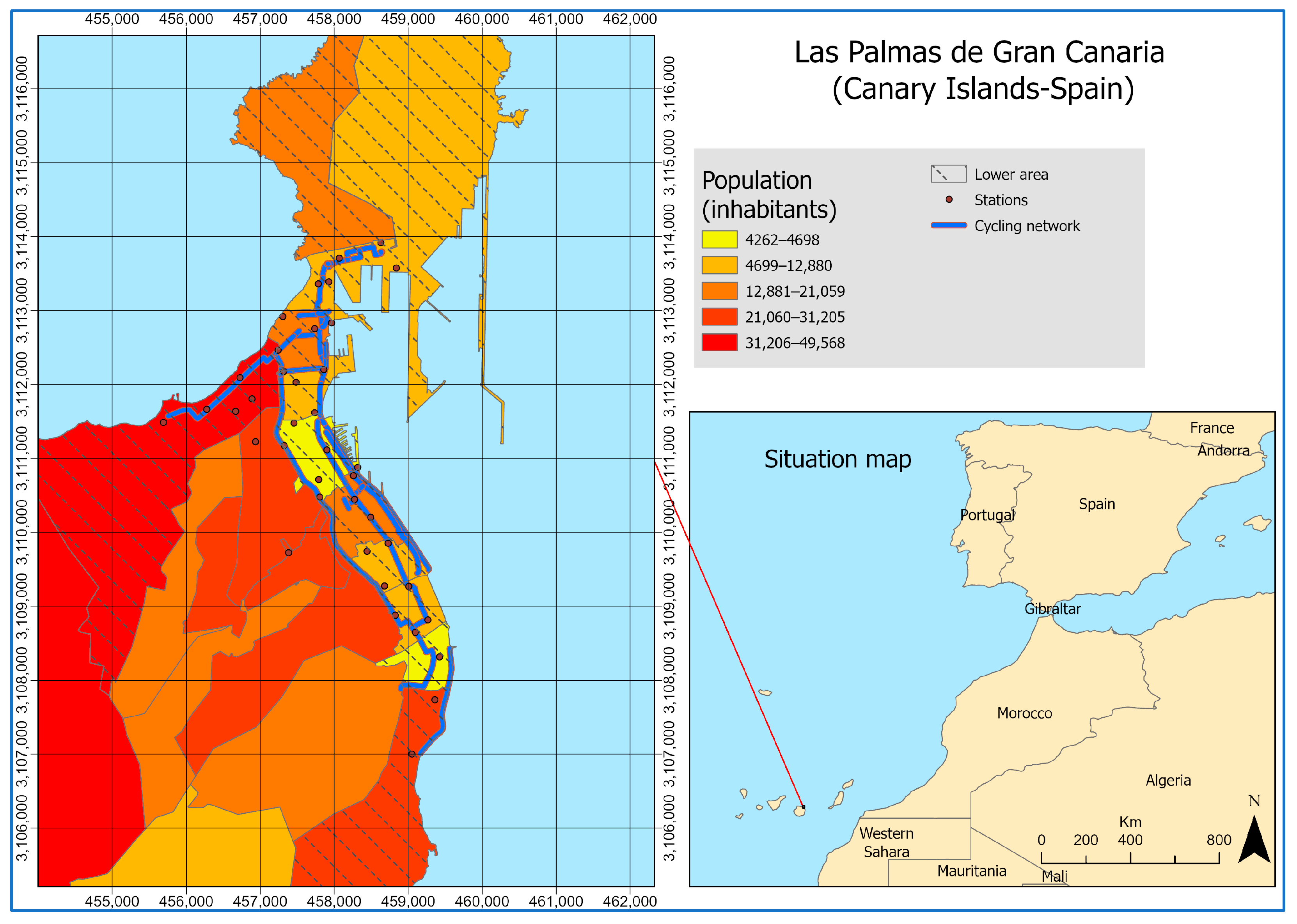
The city of Las Palmas de Gran Canaria is located on the island of Gran Canaria, one of the eight islands that make up the Canary Archipelago in the Atlantic, near the West African coast (see
Figure 1). This situation, together with the trade winds, promotes average temperatures of 20.7 °C per year, with mild winters and summers. In addition, it receives less than 300 mm of rain a year and many sunny days. Las Palmas de Gran Canaria had a population of 378,517 inhabitants in 2018, whose distribution by postal code is shown in
Figure 1.
The city’s lower part is flat. Due to its population growth, neighborhoods have been developed on the periphery, which is at a higher altitude than the city center. Specifically, the city consists of 19 neighborhoods (identified with postal codes), of which eight are located in the upper areas. The distribution of the upper and lower postal codes can be seen in
Figure 1. The population of the neighborhoods located in the upper area represents 52% of the city’s population. Las Palmas de Gran Canaria is a medium-sized, cosmopolitan city. It is also a tourist city since it is visited by numerous cruise passengers and by tourists who mostly stay in the south of the island to enjoy the sun and the beach.
The current public bicycle network in the city was put into operation in April 2018 and is described in
Figure 1. The network consists of 39 anchored bicycle stations distributed throughout the city. At present, there are only two stations in the upper area. The company Sagulpa is in charge of managing the bicycle service in Las Palmas de G.C., Sitycleta. The shared bike offer consists of 375 standard bikes and 20 electric bikes. The data show that the majority of the use of bicycles in Las Palmas de Gran Canaria is for commuting purposes rather than leisure. Therefore, offering stations close to the place of residence is essential to encouraging the use of the shared bicycle. More than 50% of the total population over 16 years of age has easy access to bike use.
The downtown area of the city of Las Palmas de Gran Canaria, due to the conditions described above, is ideal for cycling. Currently, the city is dominated by cars. For this reason, the city council has joined the initiative of more than two thousand cities in the world in promoting the use of bikes, creating bike lanes, and creating a public bike rental system. Although citizens are not used to using bikes as a regular means of transport, little by little, the number of users is increasing.
Data have been provided by the company Sagulpa, which is in charge of managing the Sitycleta network. It consists of a data set from the registry of people who rent bicycles, both local and foreign, over a period of time. Based on these data, the ArcGIS program, which is a geographic information system (GIS), has been worked on, and new variables have been created that provide information about the stations or network links. The Sitycleta rental stations have been geolocated with the ArcGIS program, and a network linking all bicycle rental points has been created.
4.1. Data
The data include all the trips of the service from the beginning of April 2018 to the end of October 2019. With respect to the trips, the following information is available: Rental time of the bike and location, customer ID, return time of the bike and location, and bike ID. Additionally, the characteristics of the customers are also considered: Birth date, language, postal zip, and gender. Nevertheless, on many occasions, these personal characteristics of the user are not available.
Trips shorter than two and a half minutes and looping trips were disregarded, while only customers residing in the city were considered. The final data set includes 105,527 trips by citizens of Las Palmas de Gran Canaria with different rental and return locations and 1976 different users.
The behavior of this group differs from those with the same rental and return station. Non-looped trips represent 95% of the total bike trips and have a mean duration of 18.4 min, which contrasts with a mean duration of 67.3 min for those with the same rental and return station. Additionally, they also differ in their use over the week. Trips with different rental and return stations are more commonplace during business days, as opposed to the other group, which is more frequent on weekends. The rental peak hours of non-looped bike trips correspond to 7–8 a.m., 13 p.m., and 17–18 p.m., while in the case of looped trips, they are 11 a.m. and 18 p.m. These facts support the assumption that looped trips tend to be leisurely. The dominant commuting use of the BSS agrees with other authors [
21,
27].
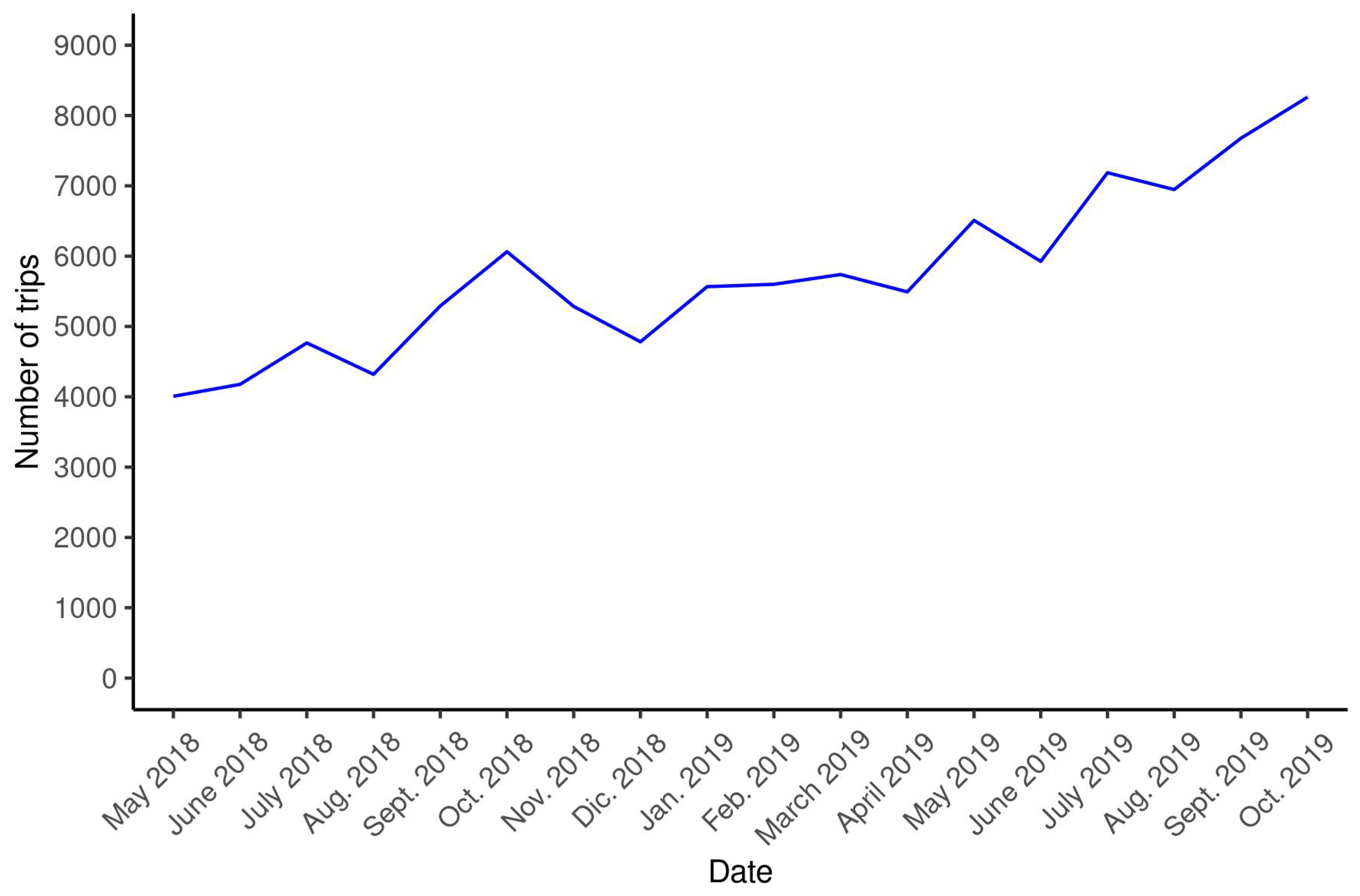
The trips on the shared bicycle network have increased over time. Specifically, when considering the group of interest, that is to say, local users with different rental and return stations, we can see in
Figure 2 that it has increased steadily over time, and no significant seasonal effect with respect to monthly periodicity can be observed.
The characteristics of the distribution of the number of trips for local customers with different rental and return stations are shown in
Table 1. A relevant percentage has used the bicycle network only once or twice since percentile 25 is 2.50% of customers who have used the bicycle 8 times or more, while 25% of customers have used the bike more than 51 times.
With respect to the trip duration, the mean duration time of the trip is 18.42 min; 25% of the trips last less than 8.2 min, while 50% of the trips last more than 12.3 min.
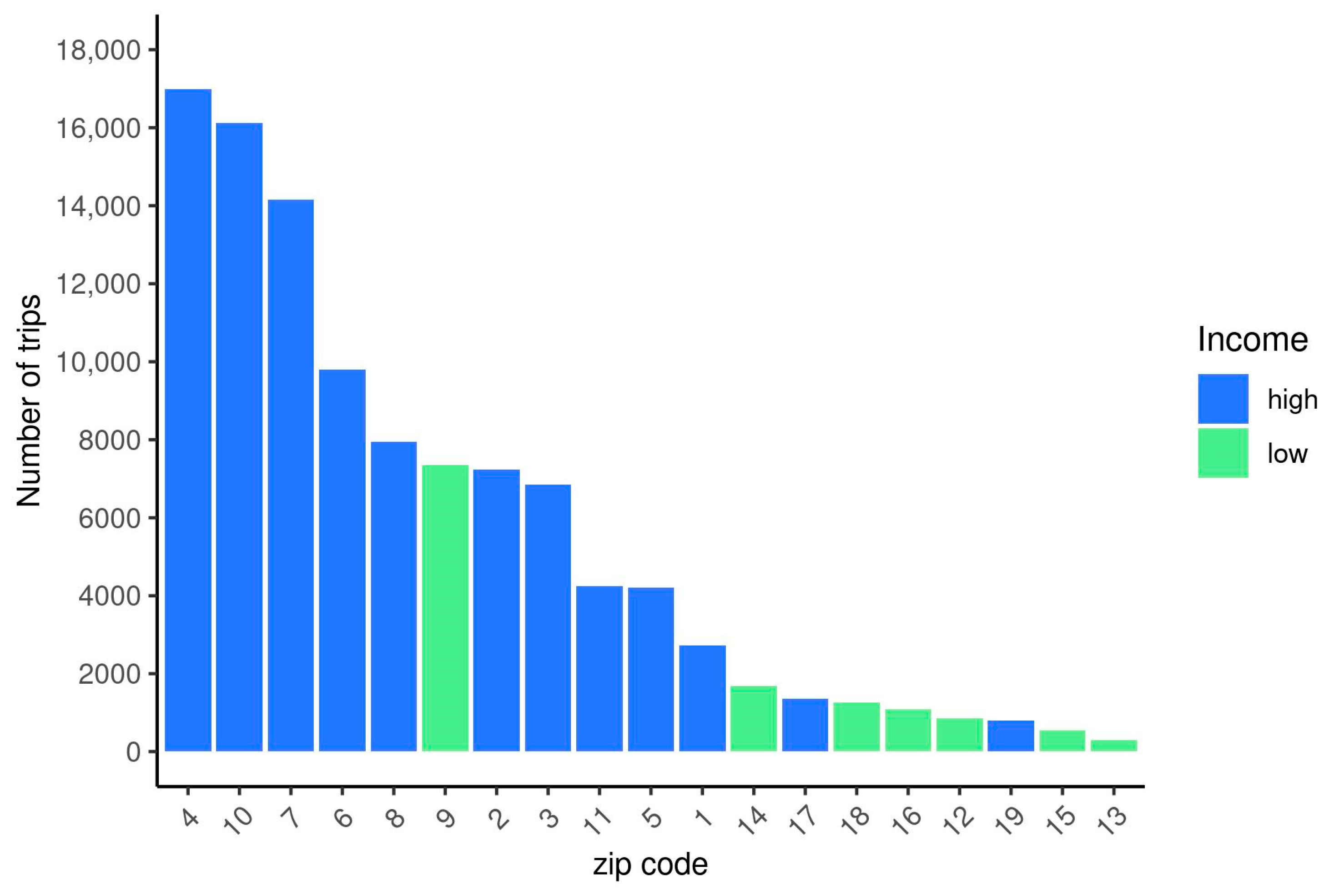
The distribution of the bike trips according to the user’s zip code is shown in
Figure 3. In general, customers who live in higher-income areas use the bike more often than others. Additionally, most of the zip codes with lower use correspond to uptown neighborhoods, many of which have no bicycle stations.
4.1.1. Characteristics of the Network
The bicycle network consists of 39 nodes, corresponding to the bicycle stations. The trips between pairs of stations are the edges of the network, and the network has been defined as undirected; that is, the direction between two stations is not relevant; only whether they are connected or not matters.
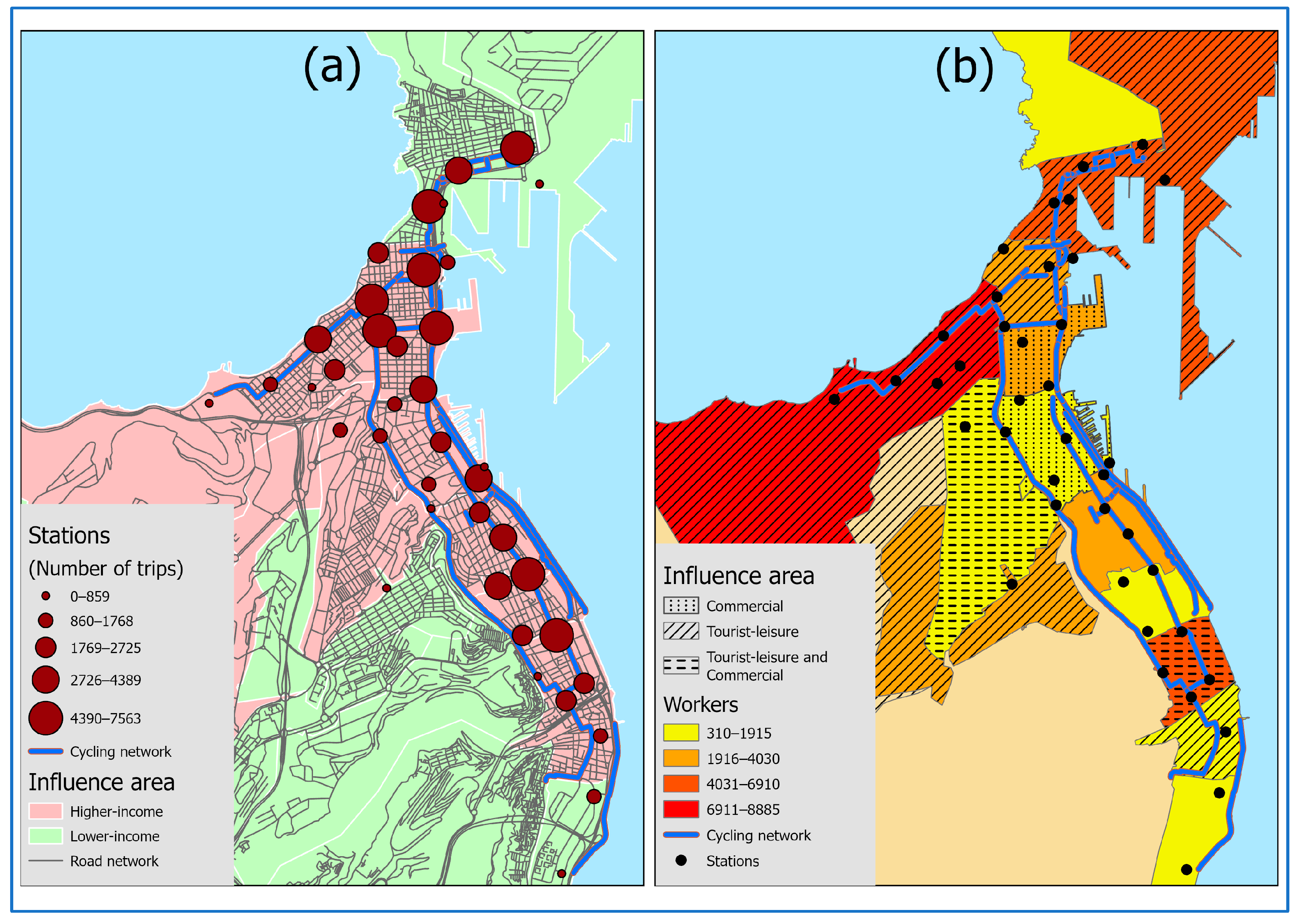
Figure 4a shows the map of the stations, the existing network of bicycle paths, and the relevance of the stations according to the number of trips at the origin station during the period of analysis. This map also presents the road/street network, which is sometimes used in combination with the bike paths to complete some trips. Additionally, zip codes with a per capita income lower than the mean are distinguished from the rest. The map shows that there is a clear geographical bias in the distribution of income. The cutoff point to distinguish higher- and lower-income zones is the mean income in the city. Of the nineteen zones in the city, ten out of twelve have stations in higher-income zones, and three out of seven have stations in lower-income zones. The map shows that most of the stations are located in higher-income zones, which correspond to the city center. Neighborhoods located far from the city center lack stations and bike paths currently. This fact is partly due to the orography of the city, which hinders the use of bikes in higher-altitude areas.
The network density is 0.93, meaning that connections represent 93% of the total possible ones in the network. Additionally, when analyzing the node centrality, we find that the degree centrality coefficient of the nodes, that is, the number of nodes connected to each node, goes from 24 to 38. The number of different bike routes available in the network is 691. The network considered is a weighted network; that is, the number of trips per route is taken into account. However, since the original weights of the network vary from 1 to 2472, the weights have been simplified to a scale from 1 to 5.
4.1.2. Characteristics of the Nodal and Edge Variables in the Network
The network includes some quantitative and qualitative variables about the stations and the variable “Distance between stations” that characterizes the alternative routes.
Table 2 shows the different variables that have been considered at the station and at the edge level.
The number of stations within a radius of 500 m for each station has been computed with the ArcGIS program after geocoding all the nodes in the network. The population within 250 m of every station has also been obtained with the ArcGIS program from population data collected from the Municipal register of inhabitants of the city of Las Palmas de Gran Canaria in 2019. Additionally, an estimation of the number of workers per postal zip, which accounts for the economic activity in each area, has been computed using a census of the commercial activities in the city, provided by the Government of the Canary Islands. The geographical distribution of the workers in the area around the cycling network is shown in
Figure 4b.
Bivariate dummy variables have also been considered: Tourist_leisure and Commercial areas show value if the zone has a tourist and/or leisure profile or a commercial area, respectively. The layout of the post codes according to these activities is presented in
Figure 4b.
A dummy variable accounting for stations located in postal zip codes with lower income has been defined (see
Figure 4a). The cut-off point of the variable was the mean income weighted by the number of tax returns filed in each zip code. Three zip codes with bicycle stations were identified as lower-income areas (35,009, 35,012, and 35,016), and six stations are in these areas. Therefore, those stations with lower income present a value of one for the variable lower income and zero otherwise.
5. Results and Discussion
The regressors included in the model may capture different effects: Structural, main nodal, interaction nodal, and relational. In this type of model, structural effects are used to control for the goodness of adjustment. The structural effects included in this model are intensity and transitivity relationships. The latter predictor belongs to the group of variables that generate dependent dyad models.
Table 3 shows the description of the predictors included in the model.
The solution to the ERGM estimators is obtained by maximum likelihood. There is no closed solution for this problem, which is why it is approximated by simulation with the Monte Carlo Markov chain (MCMC) [
13]. The model is estimated with the ERGM package of R.
The results of the ERGM estimation are shown in
Table 4, where two models are proposed. They estimate the expected probability that two bicycle stations are connected, i.e., that at least one person has taken that route irrespective of the direction taken. As observed in
Figure 4a, the sample includes an uneven distribution of stations in low- and high-income areas. Fortunately, the estimation of the coefficient for categorical variables in ERGM is robust with respect to the number of nodes belonging to every category. Then, we can interpret the significant effect of the connection of equal or different income areas independently of the distribution of low and high-income stations in the sample.
Model 1 includes the income category just as a nodal predictor; that is, in this specification, we study whether the income category in the neighborhood of a station affects the probability of generating a route irrespective of the income category of the other stations. Model 2 includes relational effects concerning the income level of the areas involved in the rental and return stations belonging to a route. In this model, the interaction between income categories involved in the rental and return stations on a route is considered. In the two models, the non-significant variables (population within a radius of 250 m) were removed from the estimation.
The structural effects in the model estimation are used as control variables. The estimation results in the two models show a negative effect of intensity, reflecting that the number of edges is lower than expected if weights are randomly distributed. Then, the network presents a higher concentration of routes among some stations than was randomly expected. The positive sign of the transitivity variable reveals a statistical trend to form triangles of connecting stations.
The estimators of the nodal effects are also stable in the two models. The concentration of stations in a given radius slightly increases the probability of connection, as expected. Due to geographical reasons, it is also expected that the up-town stations are less connected and that the distance negatively influences the probability of connection among stations [
37]. Moreover, areas with a larger number of workers are less likely to use bikes for transport. This result reveals that bikes are not very commonly used for work purposes.
Some new findings can be extracted from the estimations of the relational effects. On the one hand, the probability of connection between two stations differs depending on whether they are located in tourist-leisure areas or not. Specifically, the probability of connection between two stations located in tourist-leisure areas is greater than if they both do not belong to tourist-leisure areas (reference category). Moreover, this probability of connection between a station located in a tourist-leisure area and a second station located in a non-tourist-leisure area is also greater than in the reference case. More precisely, since coefficients in ERGM models can be interpreted as in logit models, by calculating the odds ratio, we find that the odds of two stations located in a tourist-leisure area connecting with each other are 1.13 times the case for two stations in non-tourist-leisure areas. In other words, it is 13% higher. With respect to the connection between one station in a tourist-leisure area and another one in a non-tourist-leisure area, the odds ratio is 19% higher than the reference case.
On the other hand, similar conclusions are drawn with respect to stations located in commercial areas. The probability of connection between stations located in two commercial areas is much higher than that between stations located in non-commercial areas. Specifically, the odds of two stations in commercial areas are 27% greater than the reference case (two stations in non-commercial areas). Moreover, the probability of connection when one of the stations is located in a non-commercial area also increases with respect to the reference case.
Therefore, the bike is more likely to be used in leisure and commercial areas, revealing leisure and shopping uses. The positive influence of shopping and restaurant places, together with other leisure activities, in the neighborhood on bike use was also highlighted by previous contributions [
27,
28].
When analyzing the effect of income on the probability of connection, results agree with previous literature [
2,
4,
5,
17,
20], showing that there exists a significant relationship between income and use of bike sharing. With respect to the influence of income on the probability of generating routes, Model 1 includes income as a nodal factor predictor, and results show that stations located in lower-income areas have a lower probability of connection. Specifically, their odds ratio of connection is 30% lower than stations located in higher-income zones. The fact that lower-income neighborhoods use the bike-sharing network at a lower degree agrees with the user profile of the BSS: Users are mainly individuals with higher income and education levels [
3,
4,
29]. Moreover, the results show that bike users’ preferred routes are those connecting higher-income neighborhoods, showing inequality not only in the user’s profile but in the network connectivity.
Model 2 delves into this fact by analyzing the relational effects of income and finds that the probability of connection between two stations located in zones with higher income is greater than in the case where both stations are located in zones with lower income. Quantifying the effect, we find that the odds of connecting two stations in a higher-income area are 110% greater than when both stations belong to lower-income zones. It has also been found that links between stations belonging to different income zones (higher and lower) also present a greater probability of connection than in the reference case (the odds ratio in this case is 46% higher than in the reference case).
6. Conclusions
This work contributes to the existing literature about socioeconomic equity in BSS in two aspects: On the one hand, it is the first work in this field focused on analyzing the effect of income on bike-sharing routes, as opposed to the majority of works, which focus their attention on the income just in the neighborhood of each bike station. The possibility of considering links between stations enriches the analysis and provides the manager with interesting tools for planning or developing strategies. Secondly, the methodology applied for this purpose is social network analysis, and more specifically, the ERGM estimates bike trips based on factors that influence them. This approach is also new in the context of bike-sharing literature.
As a case study, we have chosen the BSS established in Las Palmas de Gran Canaria, in the Canary Islands, Spain. The probability of connection between stations has been estimated using a weighted undirected exponential random graph model. Control variables considered are population, number of workers per zone, distance, whether stations are uptown or downtown, and type of zone (tourist-leisure, commercial, or none). Among these factors, the geographical effects show the highest influence on using bike routes. In fact, bikes in stations located in the flat area of the town are 117% more likely to be used than those in uptown. Routes, including commercial and leisure areas, are also more preferred by bike users than those connecting areas with other uses.
Socioeconomic differences are taken into account by distinguishing between higher-income and lower-income zones. Interactions between origin and return stations depending on their zone income level have also been analyzed. Two findings are shown: On the one hand, stations located in lower-income neighborhoods have a lower probability of being connected to other stations, and on the other hand, stations in higher-income areas are more likely to be connected to each other. In fact, routes connecting two stations in higher-income areas are more than twice as likely as those connecting two stations in lower-income areas. A route connecting a higher-income area and a lower-income area is 50% more likely than those connecting stations in lower-income areas as well. These findings provide knowledge of the pattern of relational behavior of the stations according to the income profile of their area.
From the above findings, some proposals can be made to managers or policymakers:
Firstly, since socioeconomic inequities are corroborated by the estimated model, managers should take this fact into account and promote policies for lower-income users. Managers could also delve into the reasons behind the socioeconomic inequities, i.e., analyze whether the annual quota represents a barrier to lower-income users or whether lower-income individuals are more reluctant to use the bicycle because of a lack of habits. Studies about the impact of equity policies on bike sharing show that their effect is sometimes lower than expected [
30]. For this reason, better knowledge about lower-income user behavior could be helpful to propose policies enhancing their use of bike sharing through price policies or habit promotion.
One of the reasons for this inequity may be the price, the access to bike stations, or the lack of habitual cycling. In the specific case of “Sitycleta”, analyzed as a case study, the price system is reasonably affordable for commuting use since it allows paying an annual quota of EUR 40, including the first thirty minutes, and fifty cents for the additional thirty minutes. So, if we want to go deeper into the facts behind this socioeconomic inequity, a survey should be delivered to users. However, if the BSS is used for leisure or casual use, prices are too expensive for users, mostly lower-income individuals. Leisure use entails longer trips, which means additional payments. Additionally, if individuals are interested in casual use, in this case, the price is too high since it is EUR 1.3 for every thirty minutes, which really represents a barrier to use.
Secondly, taking into account that our focus is on analyzing routes instead of stations, we can detect user route preferences, go deeper into the niche corresponding to users from deprived zones, and establish policies aimed at promoting and improving access to the most demanded routes. Therefore, the fact that lower-income areas connect more with higher-income areas than with other lower-income zones can be used to detect which routes should be promoted. In this sense, lower-income zones would increase their trips if access to higher-income areas was improved in terms of the quality and adequacy of bicycle paths between stations located in lower-income zones and the main higher-income zones.
Thirdly, according to the descriptive analysis, the network studied is mostly used for commuting purposes. We propose promoting bike sharing for leisure and casual use. Since prices in these cases represent a clear barrier for lower-income individuals, this promotion should entail a price policy for the lower-income group. This policy was applied in London and analyzed by [
5], who confirmed the success of the policy in leading to an increase in casual trips for lower-income users.

 ,
, 


