

The Role of Subjective Perceptions and Objective Measurements of the Urban Environment in Explaining House Prices in Greater London: A Multi-Scale Urban Morphology Analysis


Abstract
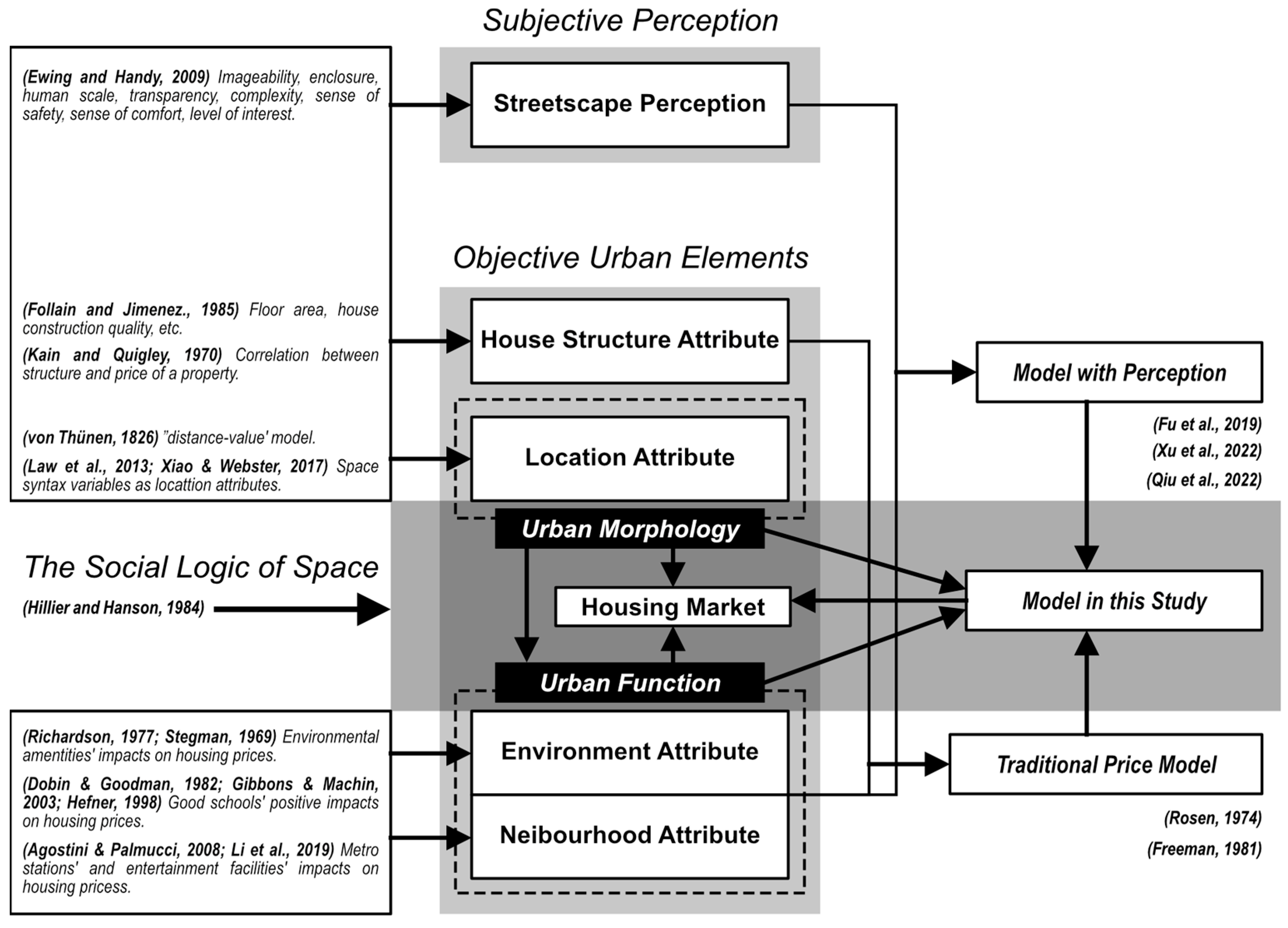
:1. Introduction
1.1. Objective Urban Dimensions in Traditional Hedonic Price Models
1.2. Subjective Perception as a New Urban Dimension Using Street View Images


| Perception Variable | Scholars | Variable Definition |
|---|---|---|
| S1. Imageability | [62] | The potential of the urban environment to evoke a strong impression on observers and whether urban elements help people to memorize and recognize them. |
| S2. Enclosure | [63,64] | A sense of closure due to the blocking of views by vertical elements in the urban environment, with walls, trees, and other vertical elements creating varying degrees of boundaries. |
| S3. Human Scale | [63,65] | The extent to which physical attributes such as the size of buildings in the urban environment match the proportions of human size. |
| S4. Transparency | [66,67] | The extent to which people can see or perceive things beyond the edge of the street, such as walls, windows, landscapes, and other boundaries. |
| S5. Complexity | [66,67] | The visual diversity of a place, which depends on the diversity of the physical environment, such as the number and type of buildings, the number and type of landscape elements, and infrastructural settings, or the abundance of human activity. |
| S6. Sense of Safety | [68] | The level of fear people have of possible crime events within the urban environment. |
| S7. Sense of Comfort | [69,70] | Commonly used to describe how comfortable people are in urban thermal environments. It is used to describe how comfortable people are when they visually perceive the urban environment in this study. |
| S8. Level of Interest | [71,72] | Frequently reflected in studies of urban point of interests describing how people like a place and how much they tend to visit it. |
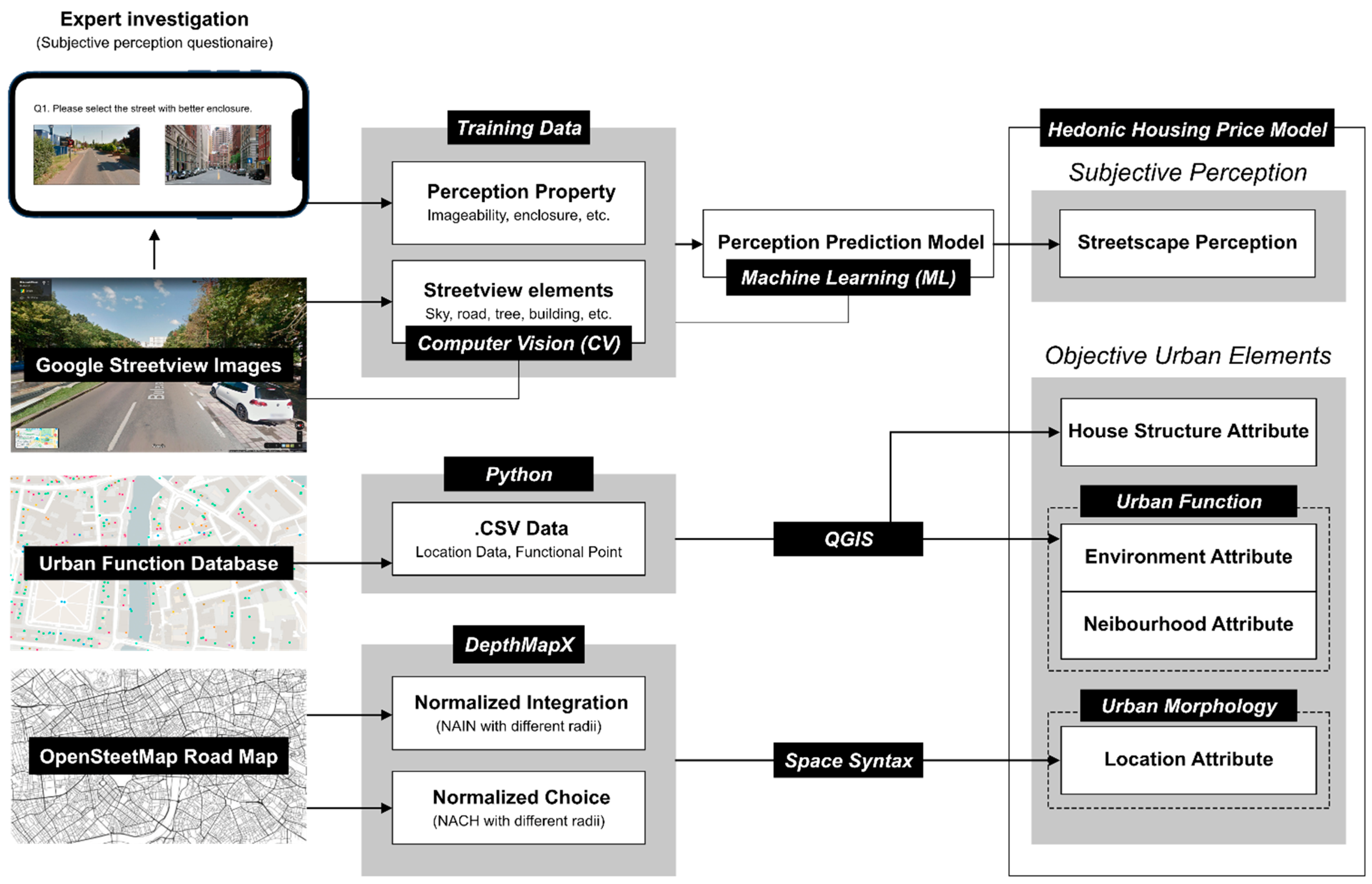
2. Materials and Method
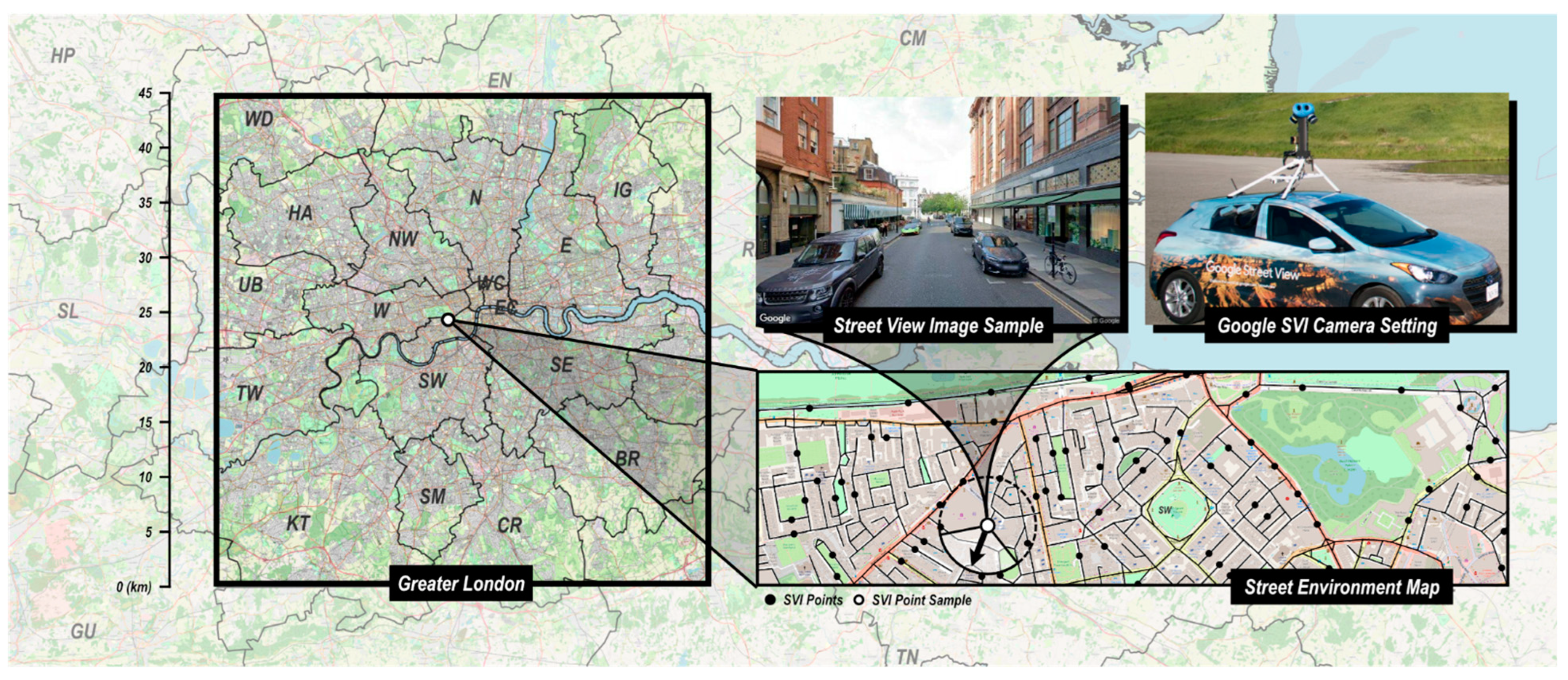
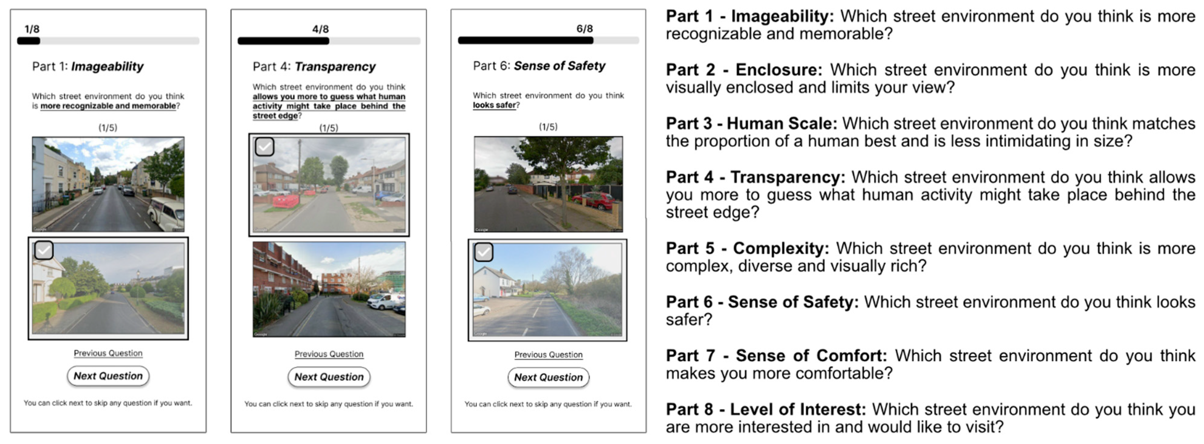
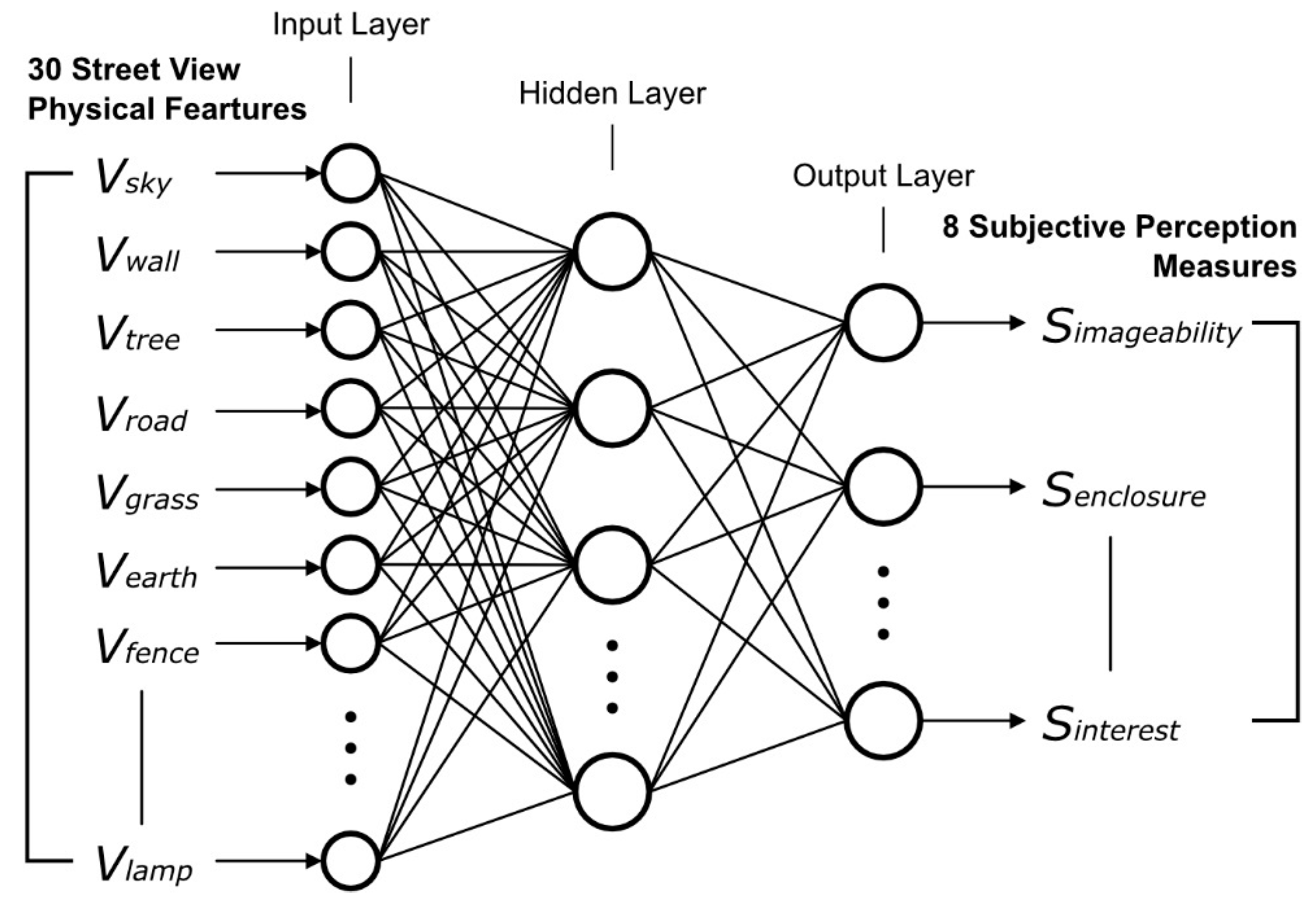
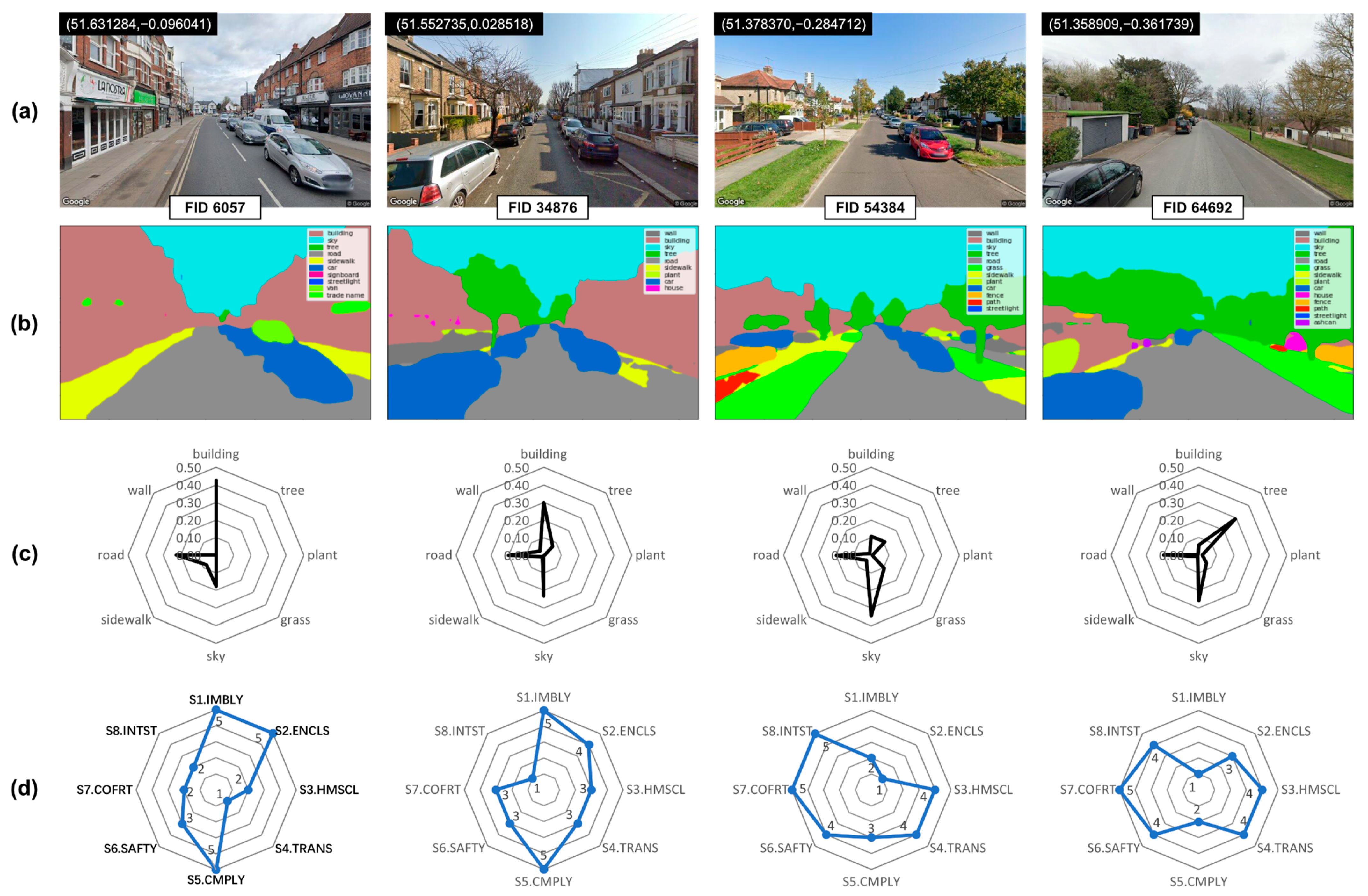
2.1. SVI, CV, and ML-Based Subjective Perception Data Collection
2.2. Hedonic House Price Model Architecture
2.2.1. Dependent Variable—House Price
2.2.2. Model Architecture
2.3. Independent Variable Data in HPM
2.3.1. House Structure Variables
2.3.2. Urban Morphology Variables
2.3.3. Urban Function Variables
3. Results
3.1. Subjective Urban Perception Prediction
3.1.1. Accuracy of the Machine Learning Prediction Model
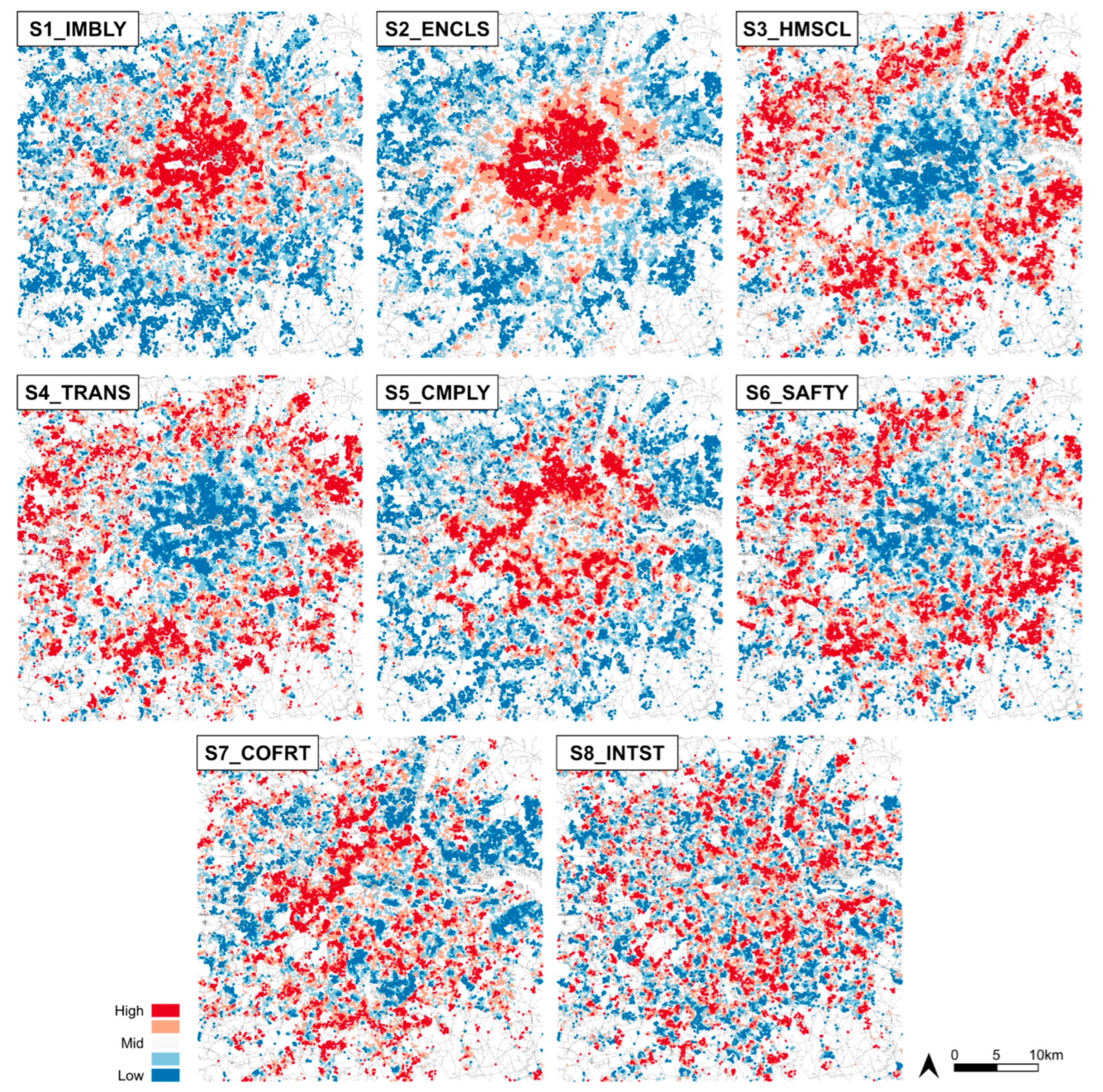
3.1.2. Spatial Heterogeneity of Urban Subjective Perception
3.2. Spatial Hedonic Price Model Result
3.2.1. Correlation of Each Attribute Group with House Prices
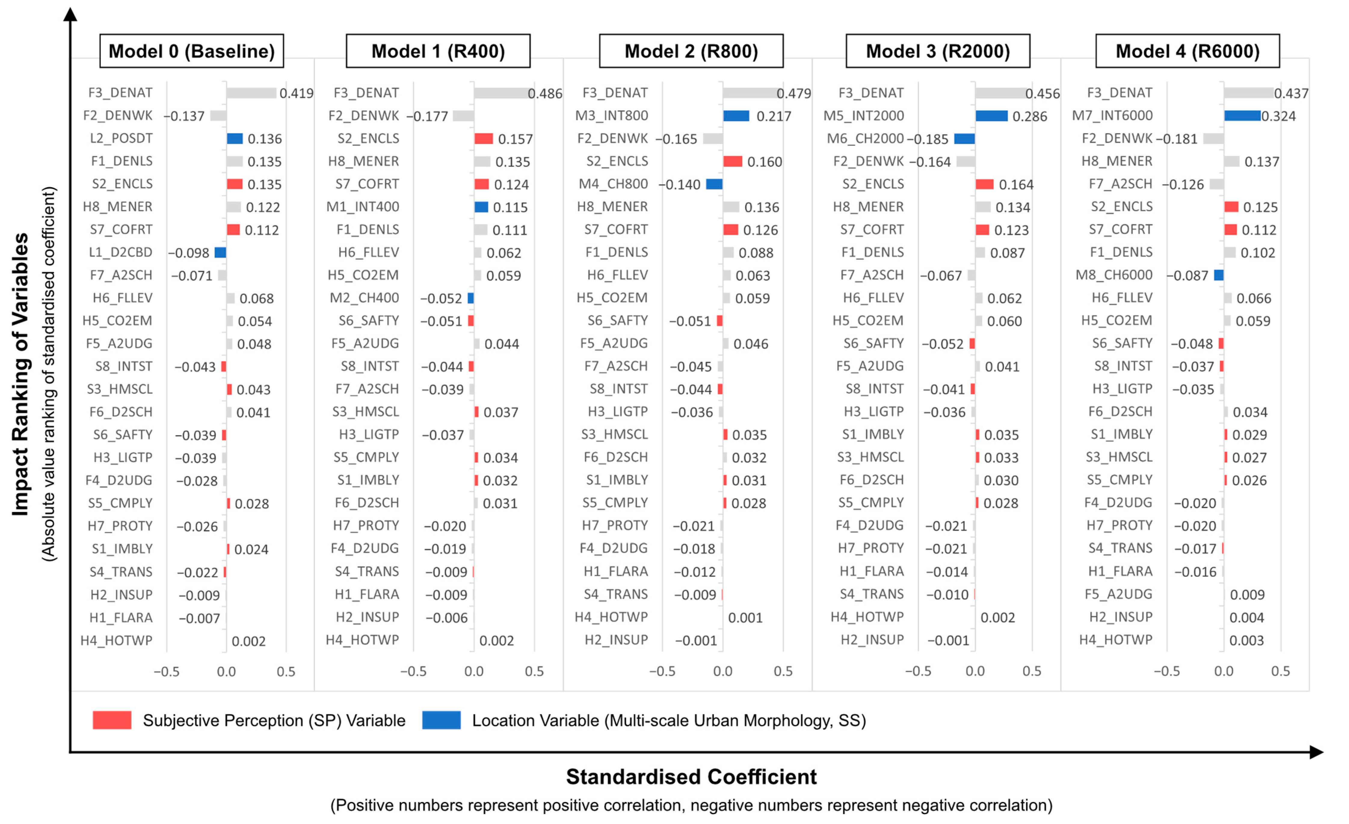
3.2.2. Results of Regression Models with Multi-Scale Urban Morphology
4. Conclusions
5. Limitation and Future Work
Author Contributions
Funding
Data Availability Statement
Conflicts of Interest
References
- Jim, C.Y.; Chen, W.Y. Impacts of urban environmental elements on residential housing prices in Guangzhou (China). Landsc. Urban Plan. 2006, 78, 422–434. [Google Scholar] [CrossRef]
- Alonso, W. Location and Land Use: Toward a General Theory of Land Rent; Harvard University Press: Cambridge, MA, USA, 1964. [Google Scholar]
- Heikkila, E.; Gordon, P.; Kim, J.I.; Peiser, R.B.; Richardson, H.W.; Dale-Johnson, D. What happened to the CBD-distance gradient? Land values in a policentric city. Environ. Plan. A 1989, 21, 221–232. [Google Scholar] [CrossRef]
- Kopczewska, K.; Lewandowska, A. The price for subway access: Spatial econometric modelling of office rental rates in London. Urban Geogr. 2018, 39, 1528–1554. [Google Scholar] [CrossRef]
- Zhang, Y.; Dong, R. Impacts of street-visible greenery on housing prices: Evidence from a hedonic price model and a massive street view image dataset in Beijing. ISPRS Int. J. Geo-Inf. 2018, 7, 104. [Google Scholar] [CrossRef] [Green Version]
- Ye, Y.; Xie, H.; Fang, J.; Jiang, H.; Wang, D. Daily accessed street greenery and housing price: Measuring economic performance of human-scale streetscapes via new urban data. Sustainability 2019, 11, 1741. [Google Scholar] [CrossRef] [Green Version]
- Boyle, A.; Barrilleaux, C.; Scheller, D. Does walkability influence housing prices? Soc. Sci. Q. 2014, 95, 852–867. [Google Scholar] [CrossRef]
- Gilderbloom, J.I.; Riggs, W.W.; Meares, W.L. Does walkability matter? An examination of walkability’s impact on housing values, foreclosures and crime. Cities 2015, 42, 13–24. [Google Scholar] [CrossRef]
- Hu, H.; Geertman, S.; Hooimeijer, P. Amenity value in post-industrial Chinese cities: The case of Nanjing. Urban Geogr. 2014, 35, 420–439. [Google Scholar] [CrossRef]
- Rosen, S. Hedonic prices and implicit markets: Product differentiation in pure competition. J. Political Econ. 1974, 82, 34–55. [Google Scholar] [CrossRef]
- Kain, J.F.; Quigley, J.M. Measuring the value of housing quality. J. Am. Stat. Assoc. 1970, 65, 532–548. [Google Scholar] [CrossRef]
- Sirmans, G.S.; MacDonald, L.; Macpherson, D.A.; Zietz, E.N. The value of housing characteristics: A meta analysis. J. Real Estate Financ. Econ. 2006, 33, 215–240. [Google Scholar] [CrossRef]
- Osland, L.; Thorsen, I. Effects on housing prices of urban attraction and labor-market accessibility. Environ. Plan. A 2008, 40, 2490–2509. [Google Scholar] [CrossRef]
- Brasington, D.M.; Hite, D. Demand for environmental quality: A spatial hedonic analysis. Reg. Sci. Urban Econ. 2005, 35, 57–82. [Google Scholar] [CrossRef] [Green Version]
- Poudyal, N.C.; Hodges, D.G.; Merrett, C.D. A hedonic analysis of the demand for and benefits of urban recreation parks. Land Use Policy 2009, 26, 975–983. [Google Scholar] [CrossRef]
- Dubin, R.A.; Goodman, A.C. Valuation of education and crime neighborhood characteristics through hedonic housing prices. Popul. Environ. 1982, 5, 166–181. [Google Scholar] [CrossRef]
- Gibbons, S.; Machin, S. Valuing English primary schools. J. Urban Econ. 2003, 53, 197–219. [Google Scholar] [CrossRef] [Green Version]
- Hillier, B.; Hanson, J. The Social Logic of Space; Cambridge University Press: Cambridge, UK, 1984. [Google Scholar]
- van Nes, A.; Yamu, C. Space Syntax: A method to measure urban space related to social, economic and cognitive factors. In The Virtual and the Real in Planning and Urban Design; Routledge: Abingdon-on-Thames, UK, 2017; pp. 136–150. [Google Scholar]
- Xiao, Y.; Webster, C. Urban Morphology and Housing Market; Springer: Berlin/Heidelberg, Germany, 2017. [Google Scholar]
- Law, S. A Multi-Scale Exploration of the Relationship Between Spatial Network Configuration and Housing Prices Using the Hedonic Price Approach: A Greater London Case Study; UCL (University College London): London, UK, 2018. [Google Scholar]
- Chan, E.T.; Schwanen, T.; Banister, D. The role of perceived environment, neighbourhood characteristics, and attitudes in walking behaviour: Evidence from a rapidly developing city in China. Transportation 2021, 48, 431–454. [Google Scholar] [CrossRef] [Green Version]
- Harvey, C. Measuring Streetscape Design for Livability Using Spatial Data and Methods; The University of Vermont and State Agricultural College: Burlington, VT, USA, 2014. [Google Scholar]
- Yin, L.; Wang, Z. Measuring visual enclosure for street walkability: Using machine learning algorithms and Google Street View imagery. Appl. Geogr. 2016, 76, 147–153. [Google Scholar] [CrossRef]
- Ito, K.; Biljecki, F. Assessing bikeability with street view imagery and computer vision. Transp. Res. Part C Emerg. Technol. 2021, 132, 103371. [Google Scholar] [CrossRef]
- Miranda, A.S.; Fan, Z.; Duarte, F.; Ratti, C. Desirable streets: Using deviations in pedestrian trajectories to measure the value of the built environment. Comput. Environ. Urban Syst. 2021, 86, 101563. [Google Scholar] [CrossRef]
- Jackson, L.E. The relationship of urban design to human health and condition. Landsc. Urban Plan. 2003, 64, 191–200. [Google Scholar] [CrossRef]
- Wolch, J.R.; Byrne, J.; Newell, J.P. Urban green space, public health, and environmental justice: The challenge of making cities ‘just green enough’. Landsc. Urban Plan. 2014, 125, 234–244. [Google Scholar] [CrossRef] [Green Version]
- Glaeser, E.L.; Kominers, S.D.; Luca, M.; Naik, N. Big data and big cities: The promises and limitations of improved measures of urban life. Econ. Inq. 2018, 56, 114–137. [Google Scholar] [CrossRef]
- Qiu, W.; Zhang, Z.; Liu, X.; Li, W.; Li, X.; Xu, X.; Huang, X. Subjective or objective measures of street environment, which are more effective in explaining housing prices? Landsc. Urban Plan. 2022, 221, 104358. [Google Scholar] [CrossRef]
- Fu, X.; Jia, T.; Zhang, X.; Li, S.; Zhang, Y. Do street-level scene perceptions affect housing prices in Chinese megacities? An analysis using open access datasets and deep learning. PLoS ONE 2019, 14, e0217505. [Google Scholar] [CrossRef] [PubMed]
- Chen, Y.; Yue, W.; La Rosa, D. Which communities have better accessibility to green space? An investigation into environmental inequality using big data. Landsc. Urban Plan. 2020, 204, 103919. [Google Scholar] [CrossRef]
- Ahmad Nia, H.; Atun, R.A. Aesthetic design thinking model for urban environments: A survey based on a review of the literature. Urban Des. Int. 2016, 21, 195–212. [Google Scholar] [CrossRef]
- Nia, H.A.; Suleiman, Y.H. Aesthetics of space organization: Lessons from traditional European cities. J. Contemp. Urban Aff. 2018, 2, 66–75. [Google Scholar] [CrossRef] [Green Version]
- Hillier, B.; Iida, S. Network and psychological effects in urban movement. In Proceedings of the Spatial Information Theory: International Conference, COSIT 2005, Ellicottville, NY, USA, 14–18 September 2005; Proceedings 7. pp. 475–490. [Google Scholar]
- Freeman, A.M. Hedonic prices, property values and measuring environmental benefits: A survey of the issues. In Measurement in Public Choice; Springer: Berlin/Heidelberg, Germany, 1981; pp. 13–32. [Google Scholar]
- Follain, J.R.; Jimenez, E. Estimating the demand for housing characteristics: A survey and critique. Reg. Sci. Urban Econ. 1985, 15, 77–107. [Google Scholar] [CrossRef]
- von Thünen, J.H. Der Isolierte Staat in Beziehung auf Landwirtschaft und Nationalökonomie; G. Fischer: Jena, Germany, 1826. [Google Scholar]
- Richardson, H.W. On the possibility of positive rent gradients. J. Urban Econ. 1977, 4, 60–68. [Google Scholar] [CrossRef]
- Stegman, M.A. Accessibility models and residential location. J. Am. Inst. Plan. 1969, 35, 22–29. [Google Scholar] [CrossRef]
- Brasington, D.M.; Hite, D.; Jauregui, A. House price impacts of racial, income, education, and age neighborhood segregation. J. Reg. Sci. 2015, 55, 442–467. [Google Scholar] [CrossRef] [Green Version]
- Agostini, C.A.; Palmucci, G.A. The anticipated capitalisation effect of a new metro line on housing prices. Fisc. Stud. 2008, 29, 233–256. [Google Scholar] [CrossRef]
- Li, H.; Wei, Y.D.; Wu, Y.; Tian, G. Analyzing housing prices in Shanghai with open data: Amenity, accessibility and urban structure. Cities 2019, 91, 165–179. [Google Scholar] [CrossRef]
- Law, S.; Karimi, K.; Penn, A.; Chiaradia, A. Measuring the influence of spatial configuration on the housing market in metropolitan London. In Proceedings of the 2013 International Space Syntax Symposium, Seoul, Republic of Korea, 31 October–3 November 2013. [Google Scholar]
- Zhang, Z.; Lu, X.; Zhou, M.; Song, Y.; Luo, X.; Kuang, B. Complex spatial morphology of urban housing price based on digital elevation model: A case study of Wuhan city, China. Sustainability 2019, 11, 348. [Google Scholar] [CrossRef] [Green Version]
- Webster, C. Pricing accessibility: Urban morphology, design and missing markets. Prog. Plan. 2010, 73, 77–111. [Google Scholar] [CrossRef]
- Song, Q.; Liu, Y.; Qiu, W.; Liu, R.; Li, M. Investigating the Impact of Perceived Micro-Level Neighborhood Characteristics on Housing Prices in Shanghai. Land 2022, 11, 2002. [Google Scholar] [CrossRef]
- Nyunt, M.S.Z.; Shuvo, F.K.; Eng, J.Y.; Yap, K.B.; Scherer, S.; Hee, L.M.; Chan, S.P.; Ng, T.P. Objective and subjective measures of neighborhood environment (NE): Relationships with transportation physical activity among older persons. Int. J. Behav. Nutr. Phys. Act. 2015, 12, 108. [Google Scholar] [CrossRef] [Green Version]
- Ewing, R.; Handy, S. Measuring the unmeasurable: Urban design qualities related to walkability. J. Urban Des. 2009, 14, 65–84. [Google Scholar] [CrossRef]
- Xu, X.; Qiu, W.; Li, W.; Liu, X.; Zhang, Z.; Li, X.; Luo, D. Associations between Street-View Perceptions and Housing Prices: Subjective vs. Objective Measures Using Computer Vision and Machine Learning Techniques. Remote Sens. 2022, 14, 891. [Google Scholar] [CrossRef]
- Qiu, W.; Li, W.; Liu, X.; Zhang, Z.; Li, X.; Huang, X. Subjective and objective measures of streetscape perceptions: Relationships with property value in Shanghai. Cities 2023, 132, 104037. [Google Scholar] [CrossRef]
- Dubey, A.; Naik, N.; Parikh, D.; Raskar, R.; Hidalgo, C.A. Deep learning the city: Quantifying urban perception at a global scale. In Proceedings of the European Conference on Computer Vision, Amsterdam, The Netherlands, 11–14 October 2016; pp. 196–212. [Google Scholar]
- Zhou, H.; He, S.; Cai, Y.; Wang, M.; Su, S. Social inequalities in neighborhood visual walkability: Using street view imagery and deep learning technologies to facilitate healthy city planning. Sustain. Cities Soc. 2019, 50, 101605. [Google Scholar] [CrossRef]
- Qiu, W.; Li, W.; Liu, X.; Huang, X. Subjectively Measured Streetscape Perceptions to Inform Urban Design Strategies for Shanghai. ISPRS Int. J. Geo-Inf. 2021, 10, 493. [Google Scholar] [CrossRef]
- Dong, L.; Jiang, H.; Li, W.; Qiu, B.; Wang, H.; Qiu, W. Assessing impacts of objective features and subjective perceptions of street environment on running amount: A case study of Boston. Landsc. Urban Plan. 2023, 235, 104756. [Google Scholar] [CrossRef]
- Su, N.; Li, W.; Qiu, W. Measuring the associations between eye-level urban design quality and on-street crime density around New York subway entrances. Habitat Int. 2023, 131, 102728. [Google Scholar] [CrossRef]
- Wang, Y.; Qiu, W.; Jiang, Q.; Li, W.; Ji, T.; Dong, L. Drivers or Pedestrians, Whose Dynamic Perceptions Are More Effective to Explain Street Vitality? A Case Study in Guangzhou. Remote Sens. 2023, 15, 568. [Google Scholar] [CrossRef]
- Tian, H.; Han, Z.; Xu, W.; Liu, X.; Qiu, W.; Li, W. Evolution of historical urban landscape with computer vision and machine learning: A case study of Berlin. J. Digit. Landsc. Arch. 2021, 16, 436–445. [Google Scholar]
- Li, X.; Zhang, C.; Li, W.; Ricard, R.; Meng, Q.; Zhang, W. Assessing street-level urban greenery using Google Street View and a modified green view index. Urban For. Urban Green. 2015, 14, 675–685. [Google Scholar] [CrossRef]
- Ma, X.; Ma, C.; Wu, C.; Xi, Y.; Yang, R.; Peng, N.; Zhang, C.; Ren, F. Measuring human perceptions of streetscapes to better inform urban renewal: A perspective of scene semantic parsing. Cities 2021, 110, 103086. [Google Scholar] [CrossRef]
- Liang, X.; Zhao, T.; Biljecki, F. Revealing spatio-temporal evolution of urban visual environments with street view imagery. Landsc. Urban Plan. 2023, 237, 104802. [Google Scholar] [CrossRef]
- Lynch, K. The Image of the City; MIT Press: Cambridge, MA, USA, 1964. [Google Scholar]
- Alexander, C. A Pattern Language: Towns, Buildings, Construction; Oxford University Press: Oxford, UK, 1977. [Google Scholar]
- Cullen, G. Concise Townscape; Routledge: Abingdon-on-Thames, UK, 2012. [Google Scholar]
- Hedman, R. Fundamentals of Urban Design; Routledge: Abingdon, Oxon, UK, 1984. [Google Scholar]
- Arnold, H. Trees in Urban Design; Van Nostrand Reinhold Co. Ltd.: Wokingham, UK, 1980. [Google Scholar]
- Jacobs, A.B. Great streets. Access Mag. 1993, 1, 23–27. [Google Scholar]
- Frevel, B. Urban safety. Ger. Policy Stud. 2006, 3, 1. [Google Scholar]
- Gómez, F.; Gil, L.; Jabaloyes, J. Experimental investigation on the thermal comfort in the city: Relationship with the green areas, interaction with the urban microclimate. Build. Environ. 2004, 39, 1077–1086. [Google Scholar] [CrossRef]
- Picot, X. Thermal comfort in urban spaces: Impact of vegetation growth: Case study: Piazza della Scienza, Milan, Italy. Energy Build. 2004, 36, 329–334. [Google Scholar] [CrossRef]
- Wu, R.; Wang, J.; Zhang, D.; Wang, S. Identifying different types of urban land use dynamics using Point-of-interest (POI) and Random Forest algorithm: The case of Huizhou, China. Cities 2021, 114, 103202. [Google Scholar] [CrossRef]
- Ying, J.J.-C.; Lu, E.H.-C.; Kuo, W.-N.; Tseng, V.S. Urban point-of-interest recommendation by mining user check-in behaviors. In Proceedings of the ACM SIGKDD International Workshop on Urban Computing, Beijing, China, 12 August 2012; pp. 63–70. [Google Scholar]
- Griew, P.; Hillsdon, M.; Foster, C.; Coombes, E.; Jones, A.; Wilkinson, P. Developing and testing a street audit tool using Google Street View to measure environmental supportiveness for physical activity. Int. J. Behav. Nutr. Phys. Act. 2013, 10, 103. [Google Scholar] [CrossRef] [Green Version]
- Kelly, C.M.; Wilson, J.S.; Baker, E.A.; Miller, D.K.; Schootman, M. Using Google Street View to audit the built environment: Interrater reliability results. Ann. Behav. Med. 2013, 45, S108–S112. [Google Scholar] [CrossRef] [Green Version]
- Queralt, A.; Molina-García, J.; Terrón-Pérez, M.; Cerin, E.; Barnett, A.; Timperio, A.; Veitch, J.; Reis, R.; Silva, A.A.P.; Ghekiere, A. Reliability of streetscape audits comparing on-street and online observations: MAPS-Global in 5 countries. Int. J. Health Geogr. 2021, 20, 6. [Google Scholar] [CrossRef]
- Wang, J.; Biljecki, F. Unsupervised machine learning in urban studies: A systematic review of applications. Cities 2022, 129, 103925. [Google Scholar] [CrossRef]
- Salesses, P.; Schechtner, K.; Hidalgo, C.A. The collaborative image of the city: Mapping the inequality of urban perception. PLoS ONE 2013, 8, e68400. [Google Scholar] [CrossRef] [Green Version]
- Herbrich, R.; Minka, T.; Graepel, T. TrueSkill™: A Bayesian skill rating system. In Proceedings of the 19th International Conference on Neural Information Processing Systems, Cambridge, MA, USA, 4–7 December 2006. [Google Scholar]
- Zhao, H.; Shi, J.; Qi, X.; Wang, X.; Jia, J. Pyramid scene parsing network. In Proceedings of the IEEE Conference on Computer Vision and Pattern Recognition, Honolulu, HI, USA, 21–26 July 2017; pp. 2881–2890. [Google Scholar]
- Lu, Y. The association of urban greenness and walking behavior: Using google street view and deep learning techniques to estimate residents’ exposure to urban greenness. Int. J. Environ. Res. Public Health 2018, 15, 1576. [Google Scholar] [CrossRef] [PubMed] [Green Version]
- Gong, Z.; Ma, Q.; Kan, C.; Qi, Q. Classifying street spaces with street view images for a spatial indicator of urban functions. Sustainability 2019, 11, 6424. [Google Scholar] [CrossRef] [Green Version]
- Zhou, H.; Liu, L.; Lan, M.; Zhu, W.; Song, G.; Jing, F.; Zhong, Y.; Su, Z.; Gu, X. Using Google Street View imagery to capture micro built environment characteristics in drug places, compared with street robbery. Comput. Environ. Urban Syst. 2021, 88, 101631. [Google Scholar] [CrossRef]
- Zhou, B.; Zhao, H.; Puig, X.; Xiao, T.; Fidler, S.; Barriuso, A.; Torralba, A. Semantic understanding of scenes through the ade20k dataset. Int. J. Comput. Vis. 2019, 127, 302–321. [Google Scholar] [CrossRef] [Green Version]
- Porzi, L.; Rota Bulò, S.; Lepri, B.; Ricci, E. Predicting and understanding urban perception with convolutional neural networks. In Proceedings of the 23rd ACM International Conference on Multimedia, Brisbane, Australia, 26–30 October 2015; pp. 139–148. [Google Scholar]
- Fu, K.; Chen, Z.; Lu, C.-T. Streetnet: Preference learning with convolutional neural network on urban crime perception. In Proceedings of the 26th ACM SIGSPATIAL International Conference on Advances in Geographic Information Systems, Seattle, WA, USA, 6–9 November 2018; pp. 269–278. [Google Scholar]
- Rumelhart, D.E.; Hinton, G.E.; Williams, R.J. Learning representations by back-propagating errors. Nature 1986, 323, 533–536. [Google Scholar] [CrossRef]
- Chi, B.; Dennett, A.; Oléron-Evans, T.; Morphet, R. A new attribute-linked residential property price dataset for England and Wales, 2011 to 2019. UCL Open Environ. Prepr. 2021, 2. [Google Scholar] [CrossRef]
- Xu, X.; Qiu, W.; Li, W.; Huang, D.; Li, X.; Yang, S. Comparing Satellite Image and GIS Data Classified Local Climate Zones to Assess Urban Heat Island: A Case Study of Guangzhou. Front. Environ. Sci. 2022, 10, 1029445. [Google Scholar] [CrossRef]
- James, G.; Witten, D.; Hastie, T.; Tibshirani, R. An Introduction to Statistical Learning; Springer: Berlin/Heidelberg, Germany, 2013; Volume 112. [Google Scholar]
- Hillier, B. Space Is the Machine: A Configurational Theory of Architecture/Bill Hillier; Cambridge University Press: New York, NY, USA, 1996. [Google Scholar]
- Narvaez, L.; Penn, A.; Griffiths, S. Spatial configuration and bid rent theory: How urban space shapes the urban economy. In Proceedings of the 2013 International Space Syntax Symposium, Seoul, Republic of Korea, 31 October–3 November 2013. [Google Scholar]
- Marcus, L. Spatial Capital: A Proposal for an Extension of Space Syntax into a More General Urban Morphology. J. Space Syntax. 2010, 1, 30–40. [Google Scholar]
- Sharmin, S.; Kamruzzaman, M. Meta-analysis of the relationships between space syntax measures and pedestrian movement. Transp. Rev. 2018, 38, 524–550. [Google Scholar] [CrossRef]
- Hillier, B.; Penn, A.; Hanson, J.; Grajewski, T.; Xu, J. Natural movement: Or, configuration and attraction in urban pedestrian movement. Environ. Plan. B Plan. Des. 1993, 20, 29–66. [Google Scholar] [CrossRef] [Green Version]
- QGIS.org. QGIS Geographic Information System. QGIS Association. 2022. Available online: http://www.qgis.org (accessed on 8 September 2022).
- Rosiers, F.D.; Thériault, M.; Voisin, M.; Dubé, J. Does an improved urban bus service affect house values? Int. J. Sustain. Transp. 2010, 4, 321–346. [Google Scholar] [CrossRef]
- Wen, H.; Xiao, Y.; Zhang, L. School district, education quality, and housing price: Evidence from a natural experiment in Hangzhou, China. Cities 2017, 66, 72–80. [Google Scholar] [CrossRef]
- Verma, D.; Jana, A.; Ramamritham, K. Predicting human perception of the urban environment in a spatiotemporal urban setting using locally acquired street view images and audio clips. Build. Environ. 2020, 186, 107340. [Google Scholar] [CrossRef]
- Kelejian, H.H.; Prucha, I.R. A generalized spatial two-stage least squares procedure for estimating a spatial autoregressive model with autoregressive disturbances. J. Real Estate Financ. Econ. 1998, 17, 99–121. [Google Scholar] [CrossRef]
- Brunsdon, C.; Fotheringham, S.; Charlton, M. Geographically weighted regression. J. R. Stat. Soc. Ser. D (Stat.) 1998, 47, 431–443. [Google Scholar] [CrossRef]


| Variable | Description | Count | Mean | Std.Dev. | Min | Max | Data Source | |
|---|---|---|---|---|---|---|---|---|
| PRICE | £/m2, dependent variable | 49,603 | 6793.59 | 3427.28 | 117.77 | 91,866.95 | LR-PPD data | |
| House Structure attribute | ||||||||
| H1_FLARA | Total floor area (m2) | 49,603 | 91.25 | 57.15 | 6.26 | 4373.00 | EPCs data | |
| H2_INSUP | House insulation performance | 49,603 | 2.58 | 1.63 | 1.00 | 5.00 | ||
| H3_LIGTP | House lighting performance | 49,603 | 3.69 | 1.52 | 1.00 | 5.00 | ||
| H4_HOTWP | House hot water performance | 49,603 | 3.80 | 0.89 | 1.00 | 5.00 | ||
| H5_CO2EM | House CO2 Emission | 49,603 | 2.00 | 1.62 | −1.40 | 66.00 | ||
| Description | Values | Count | Percent | Avg.Price | Avg.Area | Data Source | ||
| H6_FLLEV | Floor level | 1: Low | 15,959 | 32.17% | 6908.76 | 65.03 | EPCs data | |
| 2: Mid | 32,093 | 64.70% | 6698.90 | 105.08 | ||||
| 3: High | 1551 | 3.13% | 7571.03 | 74.85 | ||||
| H7_PROTY | Property type | 1: Detached | 3464 | 6.98% | 6123.85 | 174.60 | ||
| 2: Flat | 24,841 | 50.08% | 7539.41 | 67.13 | ||||
| 3: Semi | 7961 | 16.05% | 5683.22 | 113.49 | ||||
| 4: Terrace | 13,337 | 26.89% | 6244.62 | 101.24 | ||||
| H8_MENER | Main energy source | 1: Electricity | 4626 | 9.33% | 6602.96 | 63.06 | ||
| 2: Gas/LPG | 38,167 | 76.94% | 6409.88 | 97.83 | ||||
| 3: Oil/Coal | 101 | 0.20% | 6684.66 | 100.98 | ||||
| 4: Others | 6709 | 13.53% | 9111.52 | 73.11 | ||||
| Subjective urban perception variable | Count | Mean | Std.Dev. | Min | Max | Data Source | ||
| S1_IMBLY | Perceived imageability | 49,603 | 3.05 | 0.36 | 1.00 | 4.16 | SVIs, Investigation data, ML results | |
| S2_ENCLS | Perceived enclosure | 49,603 | 2.86 | 0.46 | 1.50 | 4.65 | ||
| S3_HMSCL | Perceived human scale | 49,603 | 3.06 | 0.26 | 1.00 | 4.29 | ||
| S4_TRANS | Perceived transparency | 49,603 | 2.82 | 0.20 | 2.00 | 4.00 | ||
| S5_CMPLY | Perceived complexity | 49,603 | 3.24 | 0.27 | 1.33 | 4.00 | ||
| S6_SAFTY | Perceived sense of safety | 49,603 | 3.24 | 0.22 | 1.00 | 4.50 | ||
| S7_COFRT | Perceived sense of comfort | 49,603 | 3.03 | 0.21 | 2.00 | 4.00 | ||
| S8_INTST | Perceived level of interest | 49,603 | 3.09 | 0.17 | 2.00 | 4.33 | ||
| Objective urban perception variable | Count | Mean | Std.Dev. | Min | Max | Data Source | ||
| Location Attribute (Urban morphology) | ||||||||
| L1_D2CBD | Cost network distance to CBD | 49,603 | 0.30 | 0.15 | 0.02 | 0.81 | OS data | |
| L2_POSDT | Postcode District | 49,603 | / | / | / | / | ||
| M1_INT400 | Space syntax-Integration[HH] (R400) | 49,603 | 23.18 | 6.63 | 3.56 | 68.69 | ||
| M2_CH400 | Space syntax-Choice (R400) | 49,603 | 108.54 | 59.18 | 0.00 | 902.55 | ||
| M3_INT800 | Space syntax-Integration[HH] (R800) | 49,603 | 49.09 | 20.54 | 3.56 | 176.85 | ||
| M4_CH800 | Space syntax-Choice (R800) | 49,603 | 788.61 | 485.01 | 0.00 | 6399.87 | ||
| M5_INT2000 | Space syntax-Integration[HH] (R2000) | 49,603 | 155.50 | 88.85 | 3.56 | 575.72 | ||
| M6_CH2000 | Space syntax-Choice (R2000) | 49,603 | 11,141.62 | 7914.72 | 0.00 | 47,980.45 | ||
| M7_INT6000 | Space syntax-Integration[HH] (R6000) | 49,603 | 650.86 | 459.06 | 3.56 | 2148.27 | ||
| M8_CH6000 | Space syntax-Choice (R6000) | 49,603 | 272,714.0 | 249,841.4 | 0.00 | 1,552,460 | ||
| Neighbourhood and Environment Attribute (Urban Functional Property) | ||||||||
| F1_DENLS | Density of urban services (within 1 km) | 49,603 | 341.28 | 384.77 | 0.00 | 5515.00 | OS data | |
| F2_DENWK | Density of workplace (within 1 km) | 49,603 | 337.43 | 463.93 | 1.00 | 5880.00 | ||
| F3_DENAT | Density of attraction (within 1 km) | 49,603 | 27.36 | 40.80 | 0.00 | 572.00 | ||
| F4_D2UDG | Distance to TfL station (km) | 49,603 | 0.75 | 0.58 | 0.00 | 7.26 | TfL data | |
| F5_A2UDG | Accessibility to TfL station (within 3km) | 49,603 | 15.94 | 13.04 | 0.00 | 70.00 | ||
| F6_D2SCH | Distance to quality school (km) | 49,603 | 0.56 | 0.40 | 0.00 | 6.94 | Ofsted data | |
| F7_A2SCH | Accessibility to quality school (within 3 km) | 49,603 | 24.93 | 14.76 | 0.00 | 83.00 | ||
| Perception | Accuracy | Precision | Recall | F1-Score | Criteria |
|---|---|---|---|---|---|
| S1. Imageability | 0.710 | 0.731 | 0.725 | 0.721 | Good |
| S2. Enclosure | 0.643 | 0.630 | 0.666 | 0.629 | Moderate |
| S3. Human Scale | 0.795 | 0.785 | 0.780 | 0.779 | Good |
| S4. Transparency | 0.722 | 0.723 | 0.732 | 0.724 | Good |
| S5. Complexity | 0.579 | 0.628 | 0.613 | 0.613 | Moderate |
| S6. Sense of Safety | 0.652 | 0.657 | 0.664 | 0.659 | Moderate |
| S7. Sense of Comfort | 0.720 | 0.726 | 0.732 | 0.716 | Good |
| S8. Level of Interest | 0.711 | 0.737 | 0.724 | 0.729 | Good |
| OLS Diagnosis | House Structure Attributes | Location Attributes (Urban Morphology) | Neighborhood Attributes (Urban Function) | Subjective Perception Scores |
|---|---|---|---|---|
| Adjusted R2 | 0.085 *** | 0.427 *** | 0.342 *** | 0.342 *** |
| Pr. (F-statistic) | 0.000 *** | 0.000 *** | 0.000 *** | 0.000 *** |
| Model 0 | Model 1 | Model 2 | Model 3 | Model 4 | ||||||
|---|---|---|---|---|---|---|---|---|---|---|
| Location Attribute | Baseline (L1, L2) | M1, M2 (R400) | M3, M4 (R800) | M5, M6 (R2000) | M7, M8 (R6000) | |||||
| Adjusted R2 | 0.496 | *** | 0.482 | *** | 0.484 | *** | 0.486 | *** | 0.494 | *** |
| Pr. (F-statistic) | 0.000 | *** | 0.000 | *** | 0.000 | *** | 0.000 | *** | 0.000 | *** |
| Variable | Coef. | P > t | Coef. | P > t | Coef. | P > t | Coef. | P > t | Coef. | P > t |
| CONSTANT | *** | *** | *** | *** | *** | |||||
| House Structure attribute | ||||||||||
| H1_FLARA | −0.007 | −0.009 | ** | −0.012 | ** | −0.014 | ** | −0.016 | *** | |
| H2_INSUP | −0.009 | ** | −0.006 | −0.001 | −0.001 | 0.004 | ||||
| H3_LIGTP | −0.039 | *** | −0.037 | *** | −0.036 | *** | −0.036 | *** | −0.035 | *** |
| H4_HOTWP | 0.002 | 0.002 | 0.001 | 0.002 | 0.003 | |||||
| H5_CO2EM | 0.054 | *** | 0.059 | *** | 0.059 | *** | 0.06 | *** | 0.059 | *** |
| H6_FLLEV | 0.068 | *** | 0.062 | *** | 0.063 | *** | 0.062 | *** | 0.066 | *** |
| H7_PROTY | −0.026 | *** | −0.02 | *** | −0.021 | *** | −0.021 | *** | −0.02 | *** |
| H8_MENER | 0.122 | *** | 0.135 | *** | 0.136 | *** | 0.134 | *** | 0.137 | *** |
| Subjective urban perception variable | ||||||||||
| S1_IMBLY | 0.024 | *** | 0.032 | *** | 0.031 | *** | 0.035 | *** | 0.029 | *** |
| S2_ENCLS | 0.135 | *** | 0.157 | *** | 0.16 | *** | 0.164 | *** | 0.125 | *** |
| S3_HMSCL | 0.043 | *** | 0.037 | *** | 0.035 | *** | 0.033 | *** | 0.027 | *** |
| S4_TRANS | −0.022 | *** | −0.009 | *** | −0.009 | *** | −0.01 | *** | −0.017 | *** |
| S5_CMPLY | 0.028 | *** | 0.034 | *** | 0.028 | *** | 0.028 | *** | 0.026 | *** |
| S6_SAFTY | −0.039 | *** | −0.051 | *** | −0.051 | *** | −0.052 | *** | −0.048 | *** |
| S7_COFRT | 0.112 | *** | 0.124 | *** | 0.126 | *** | 0.123 | *** | 0.112 | *** |
| S8_INTST | −0.043 | *** | −0.044 | *** | −0.044 | *** | −0.041 | *** | −0.037 | *** |
| Objective urban perception variable | ||||||||||
| Location Attribute (Urban Morphology) | ||||||||||
| L1_D2CBD | −0.098 | *** | / | / | / | / | ||||
| L2_POSDT | 0.136 | *** | / | / | / | / | ||||
| M1_INT400 | / | 0.115 | *** | / | / | / | ||||
| M2_CH400 | / | −0.052 | *** | / | / | / | ||||
| M3_INT800 | / | / | 0.217 | *** | / | / | ||||
| M4_CH800 | / | / | −0.14 | *** | / | / | ||||
| M5_INT2000 | / | / | / | 0.286 | *** | / | ||||
| M6_CH2000 | / | / | / | −0.185 | *** | / | ||||
| M7_INT6000 | / | / | / | / | 0.324 | *** | ||||
| M8_CH6000 | / | / | / | / | −0.087 | *** | ||||
| Neighborhood Attribute (Urban Functional Property) | ||||||||||
| F1_DENLS | 0.135 | *** | 0.111 | *** | 0.088 | *** | 0.087 | *** | 0.102 | *** |
| F2_DENWK | −0.137 | *** | −0.177 | *** | −0.165 | *** | −0.164 | *** | −0.181 | *** |
| F3_DENAT | 0.419 | *** | 0.486 | *** | 0.479 | *** | 0.456 | *** | 0.437 | *** |
| F4_D2UDG | −0.028 | *** | −0.019 | *** | −0.018 | *** | −0.021 | *** | −0.02 | *** |
| F5_A2UDG | 0.048 | *** | 0.044 | *** | 0.046 | *** | 0.041 | *** | 0.009 | *** |
| F6_D2SCH | 0.041 | *** | 0.031 | *** | 0.032 | *** | 0.03 | *** | 0.034 | *** |
| F7_A2SCH | −0.071 | *** | −0.039 | *** | −0.045 | *** | −0.067 | *** | −0.126 | *** |
Disclaimer/Publisher’s Note: The statements, opinions and data contained in all publications are solely those of the individual author(s) and contributor(s) and not of MDPI and/or the editor(s). MDPI and/or the editor(s) disclaim responsibility for any injury to people or property resulting from any ideas, methods, instructions or products referred to in the content. |
© 2023 by the authors. Licensee MDPI, Basel, Switzerland. This article is an open access article distributed under the terms and conditions of the Creative Commons Attribution (CC BY) license (https://creativecommons.org/licenses/by/4.0/).
Share and Cite
Yang, S.; Krenz, K.; Qiu, W.; Li, W. The Role of Subjective Perceptions and Objective Measurements of the Urban Environment in Explaining House Prices in Greater London: A Multi-Scale Urban Morphology Analysis. ISPRS Int. J. Geo-Inf. 2023, 12, 249. https://doi.org/10.3390/ijgi12060249
Yang S, Krenz K, Qiu W, Li W. The Role of Subjective Perceptions and Objective Measurements of the Urban Environment in Explaining House Prices in Greater London: A Multi-Scale Urban Morphology Analysis. ISPRS International Journal of Geo-Information. 2023; 12(6):249. https://doi.org/10.3390/ijgi12060249
Chicago/Turabian StyleYang, Sijie, Kimon Krenz, Waishan Qiu, and Wenjing Li. 2023. "The Role of Subjective Perceptions and Objective Measurements of the Urban Environment in Explaining House Prices in Greater London: A Multi-Scale Urban Morphology Analysis" ISPRS International Journal of Geo-Information 12, no. 6: 249. https://doi.org/10.3390/ijgi12060249