


Using Enhanced Gap-Filling and Whittaker Smoothing to Reconstruct High Spatiotemporal Resolution NDVI Time Series Based on Landsat 8, Sentinel-2, and MODIS Imagery

 , ,
, ,
Abstract
:1. Introduction
2. Study Area and Data
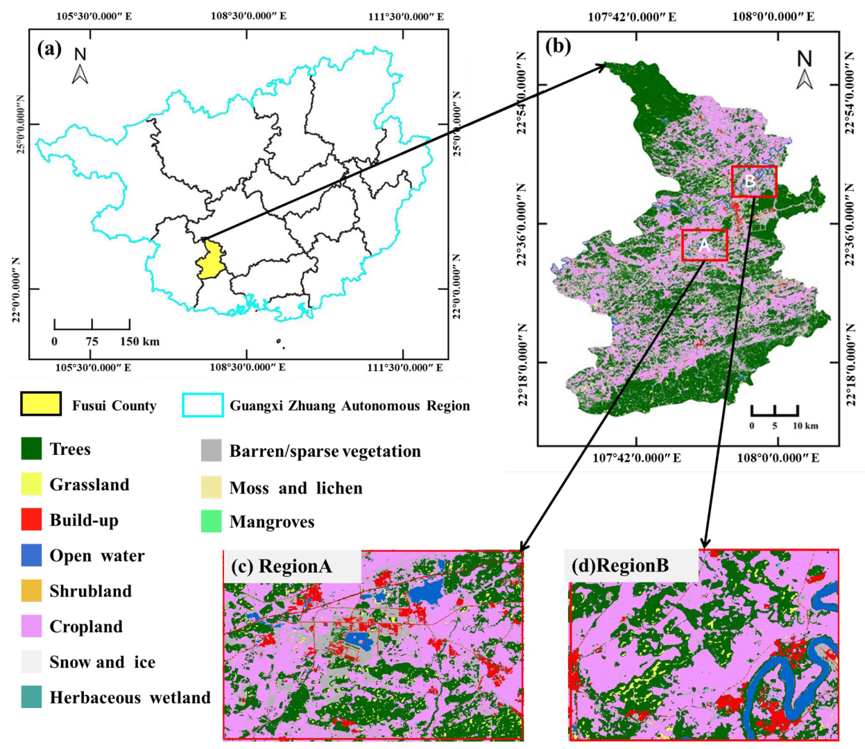
2.1. Study Area
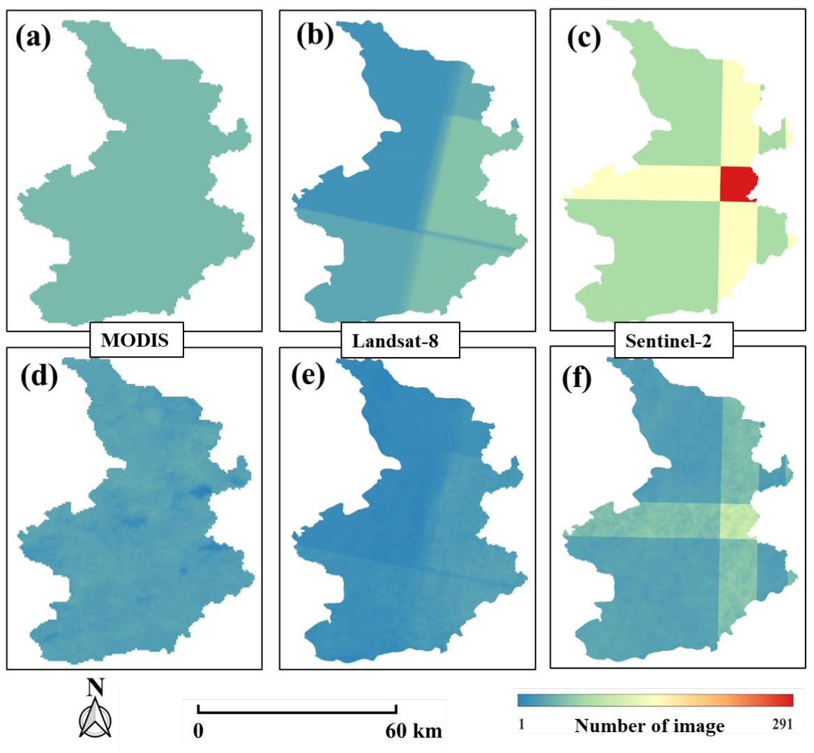
2.2. Data
2.2.1. MODIS Image Collection
2.2.2. Landsat-8 Image Collection
2.2.3. Sentinel-2 Image Collection
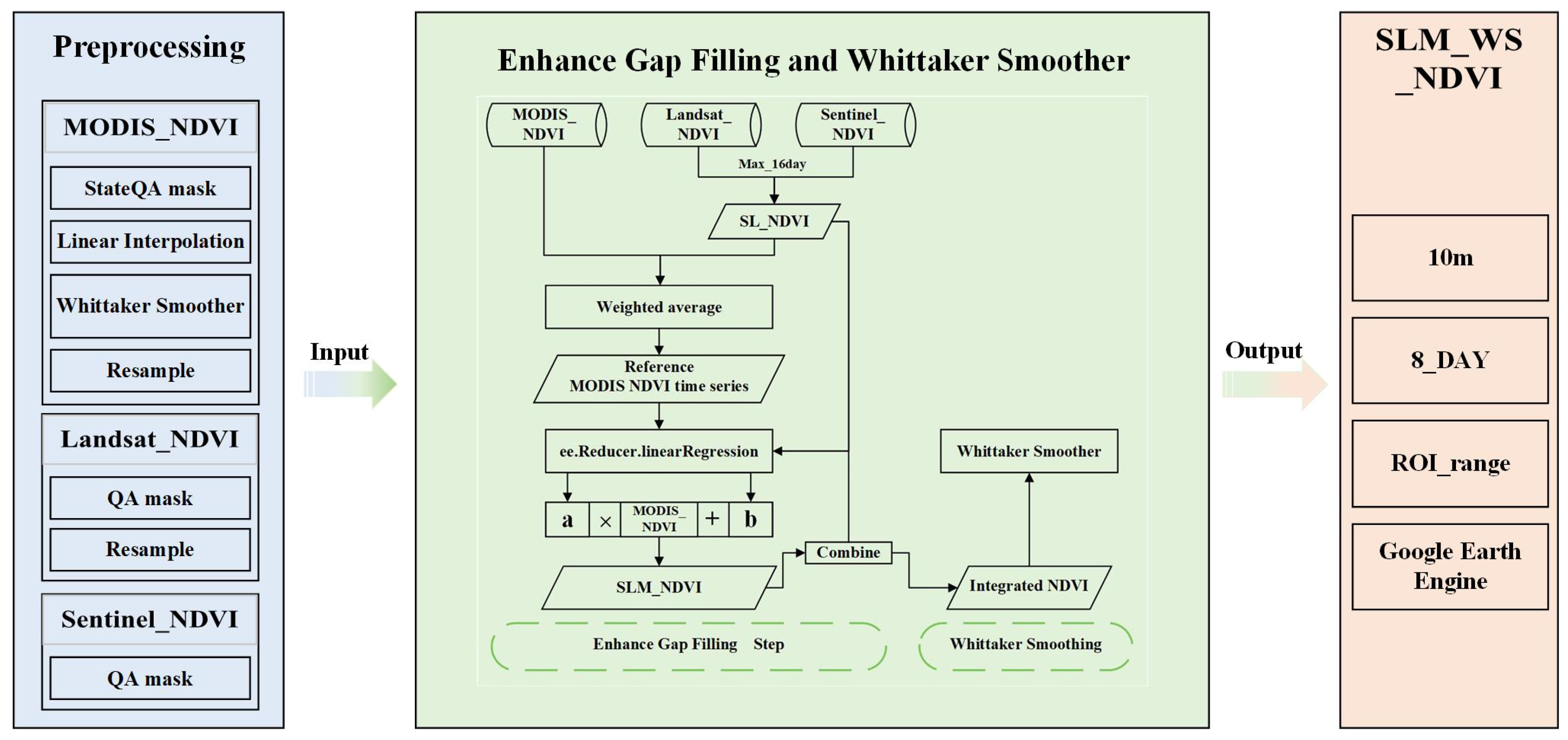
3. Methodology
3.1. Preprocessing
3.2. Enhance Gap-Filling
3.3. Whittaker Smoothing
3.4. Accuracy Metrics
4. Results
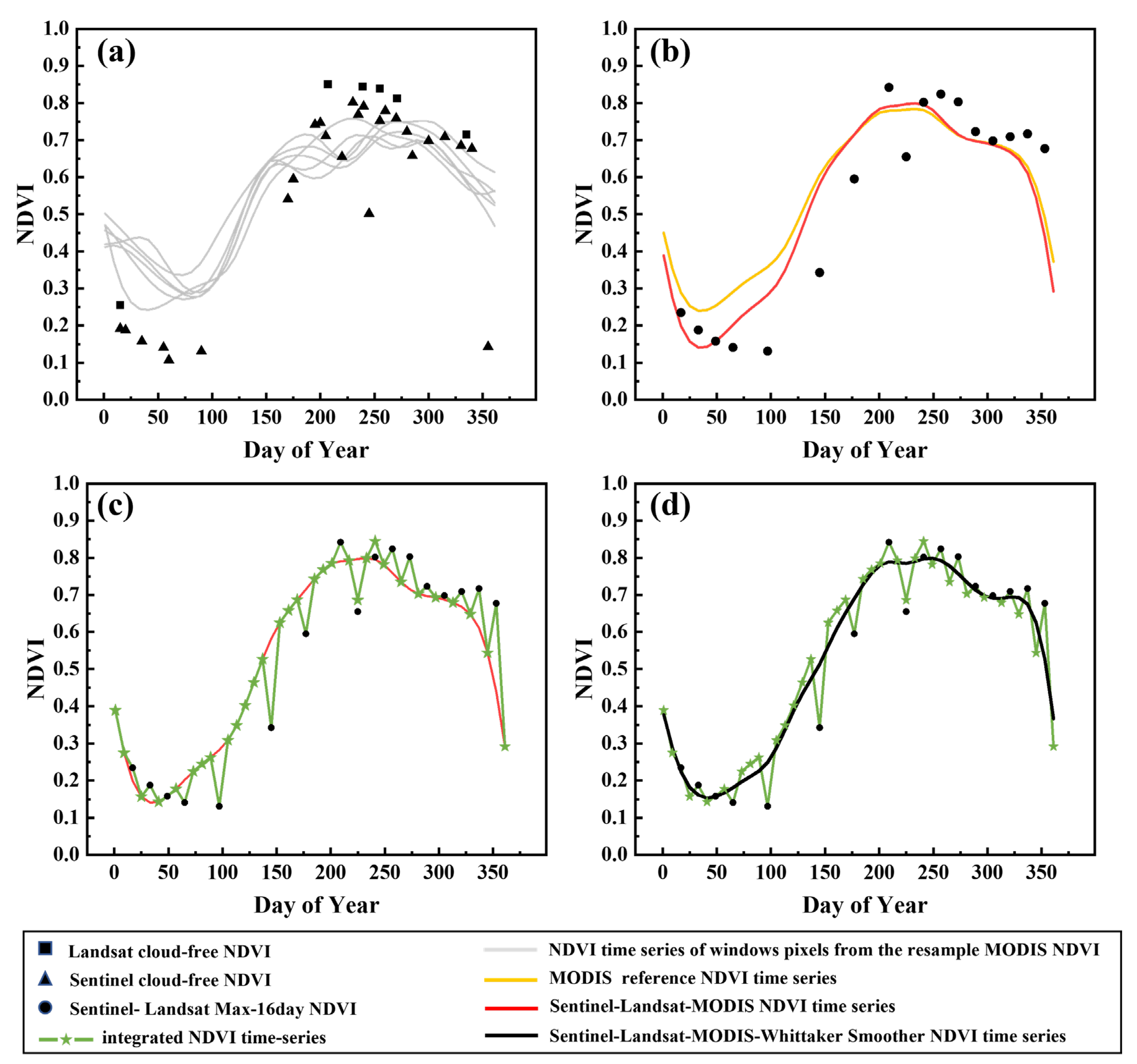
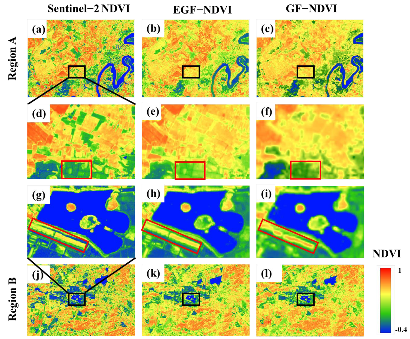
4.1. Qualitative Assessment
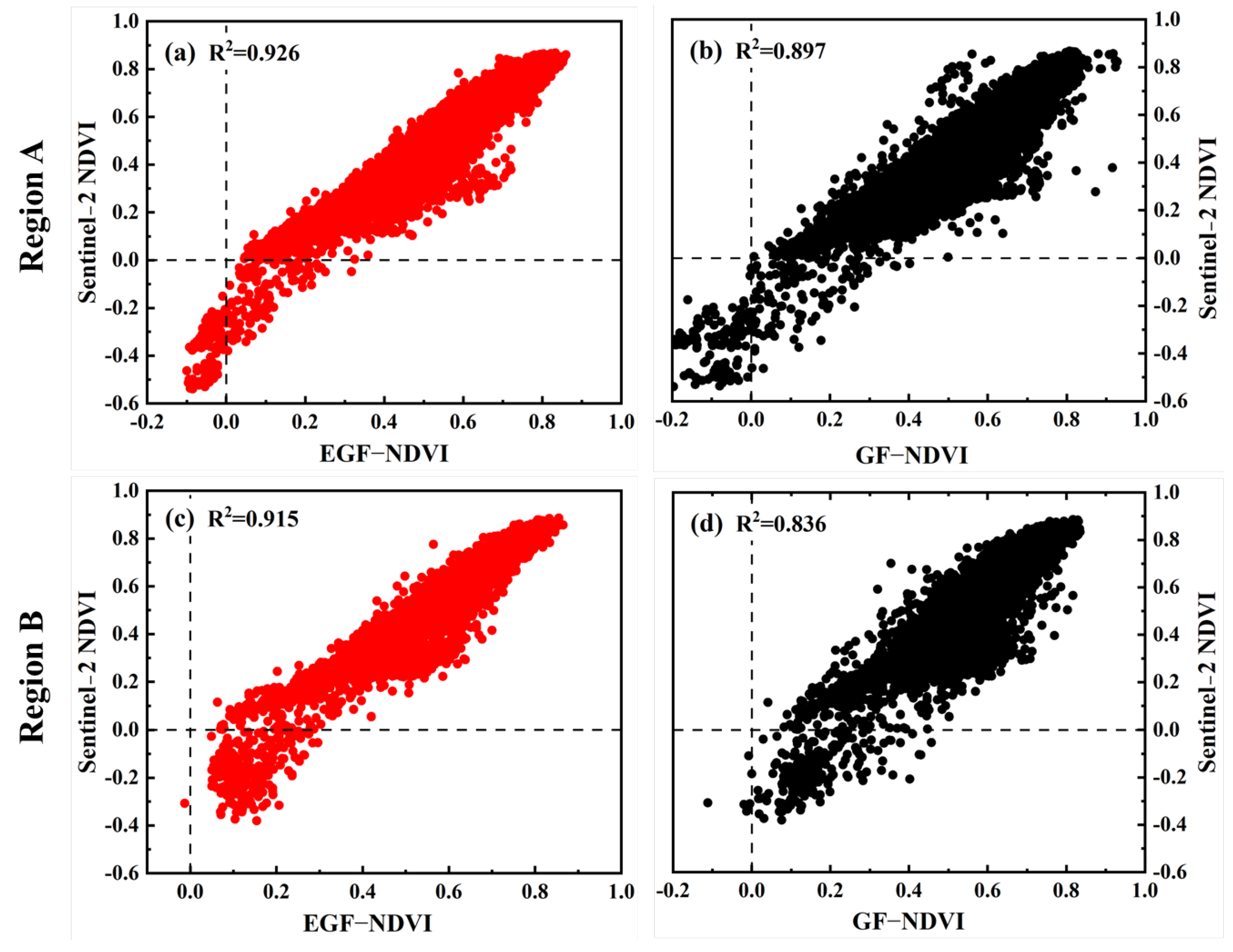
4.2. Quantitative Assessment
5. Discussion
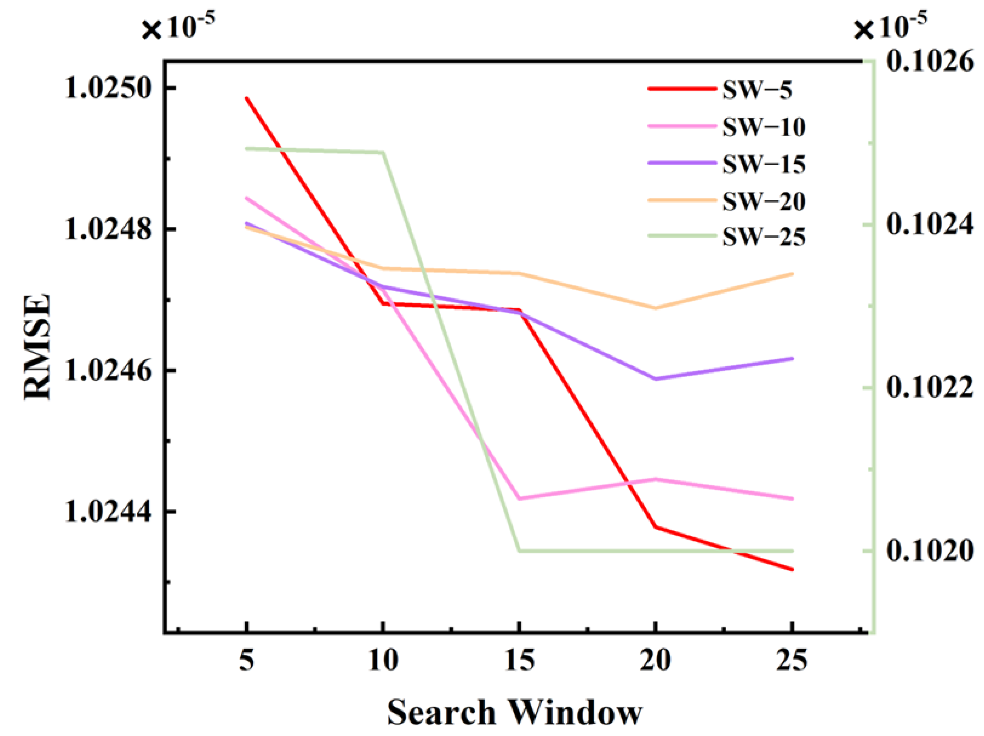
5.1. Parameter Determination of the Window Size
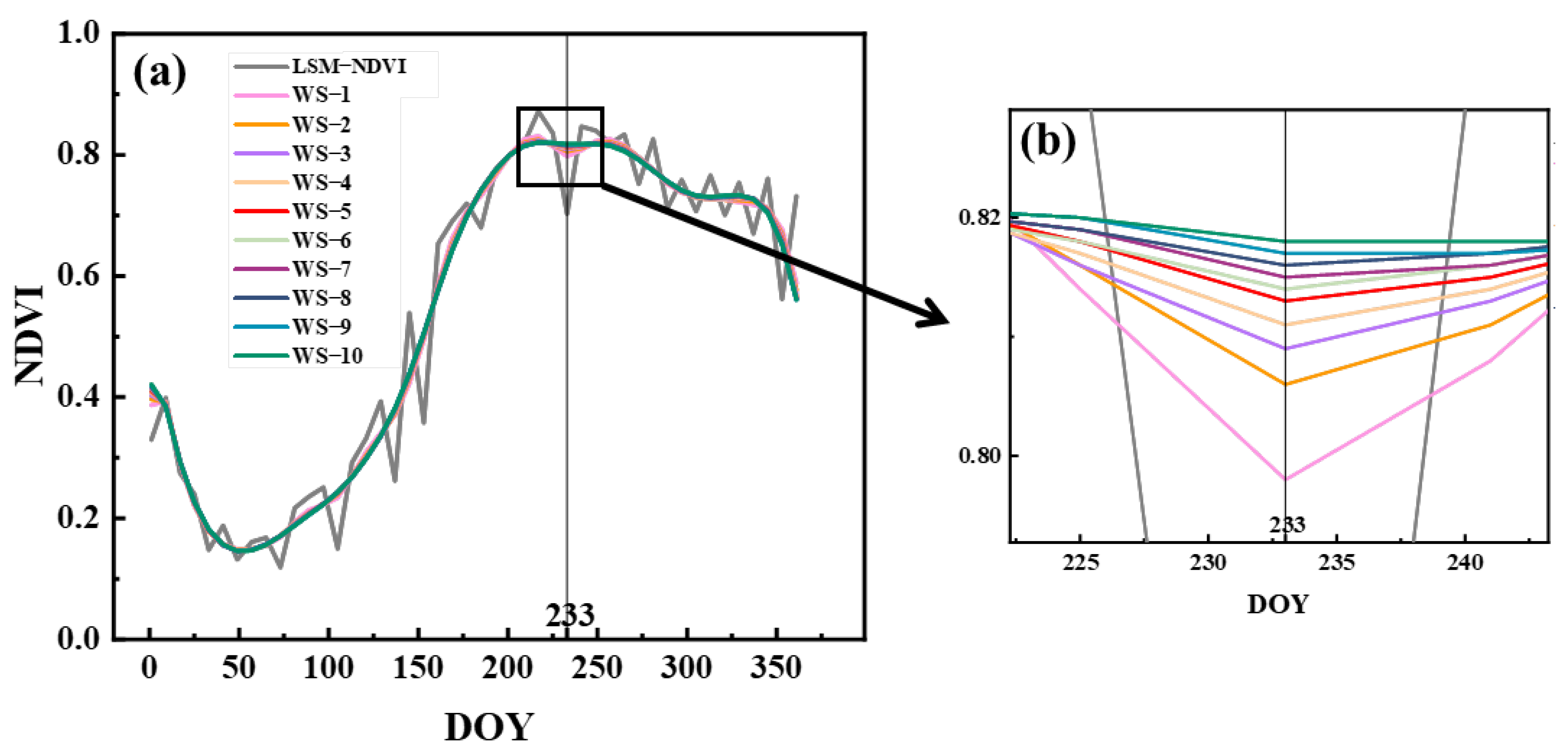
5.2. Parameter Determination of the Whittaker Smoothing
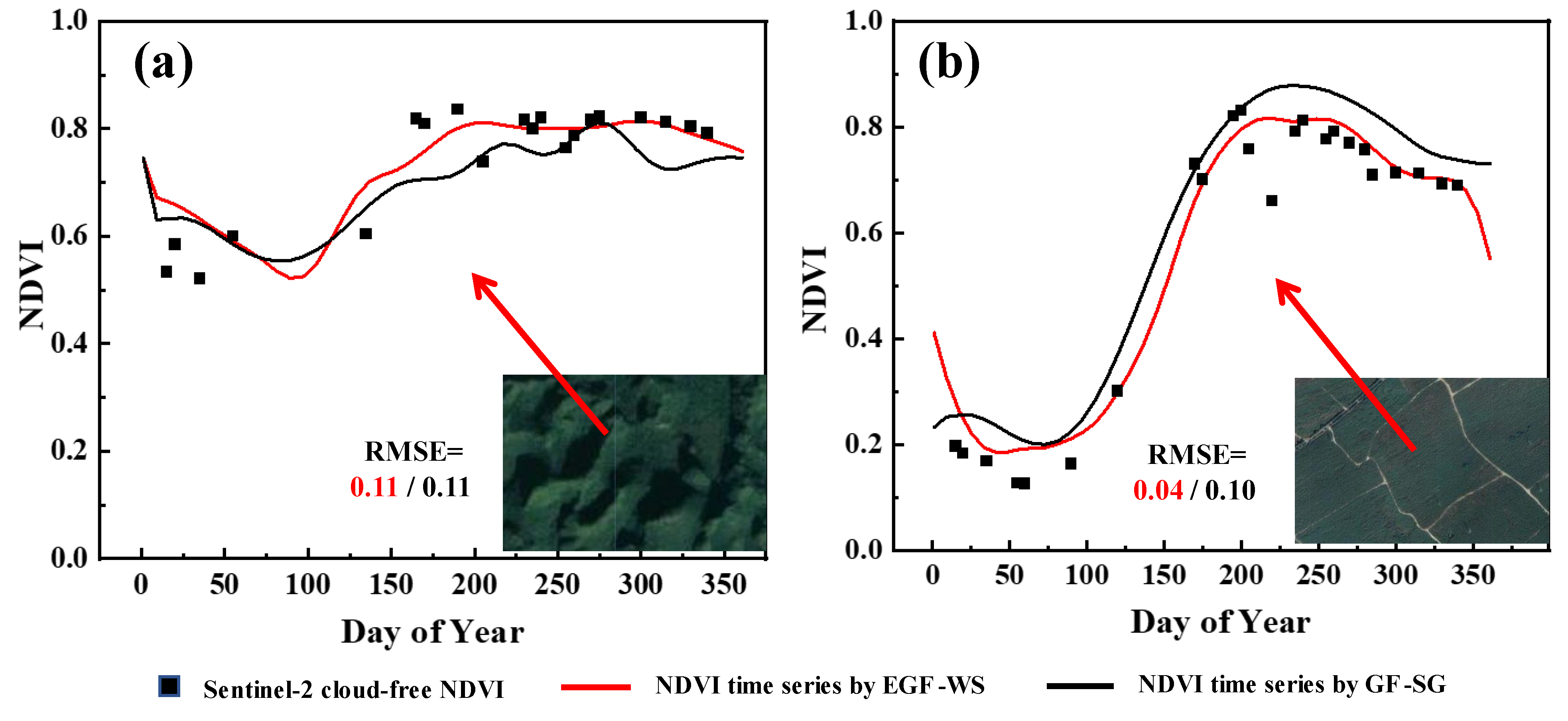
5.3. Performance Metrics and Statistical Metrics
5.4. Advantages and Limitations of the EGF-WS Method
6. Conclusions
Author Contributions
Funding
Institutional Review Board Statement
Informed Consent Statement
Data Availability Statement
Acknowledgments
Conflicts of Interest
References
- Wang, J.; Xiao, X.; Liu, L.; Wu, X.; Qin, Y.; Steiner, J.L.; Dong, J. Mapping sugarcane plantation dynamics in Guangxi, China, by time series Sentinel-1, Sentinel-2 and Landsat images. Remote Sens. Environ. 2020, 247, 111951. [Google Scholar] [CrossRef]
- Lyle, G.; Clarke, K.; Kilpatrick, A.; Summers, D.M.; Ostendorf, B. A Spatial and Temporal Evaluation of Broad-Scale Yield Predictions Created from Yield Mapping Technology and Landsat Satellite Imagery in the Australian Mediterranean Dryland Cropping Region. ISPRS Int. J. Geo-Inf. 2023, 12, 50. [Google Scholar] [CrossRef]
- Ghorbanian, A.; Mohammadzadeh, A.; Jamali, S. Linear and Non-Linear Vegetation Trend Analysis throughout Iran Using Two Decades of MODIS NDVI Imagery. Remote Sens. 2022, 14, 3683. [Google Scholar] [CrossRef]
- Mashhadi, N.; Alganci, U. Evaluating BFASTMonitor Algorithm in Monitoring Deforestation Dynamics in Coniferous and Deciduous Forests with LANDSAT Time Series: A Case Study on Marmara Region, Turkey. ISPRS Int. J. Geo-Inf. 2022, 11, 573. [Google Scholar] [CrossRef]
- Liu, L.; Cao, R.; Chen, J.; Shen, M.; Wang, S.; Zhou, J.; He, B. Detecting crop phenology from vegetation index time-series data by improved shape model fitting in each phenological stage. Remote Sens. Environ. 2022, 277, 113060. [Google Scholar] [CrossRef]
- Guo, Y.; Xia, H.; Pan, L.; Zhao, X.; Li, R.; Bian, X.; Wang, R.; Yu, C. Development of a New Phenology Algorithm for Fine Mapping of Cropping Intensity in Complex Planting Areas Using Sentinel-2 and Google Earth Engine. ISPRS Int. J. Geo-Inf. 2021, 10, 587. [Google Scholar] [CrossRef]
- Aksoy, H.; Cetin, M.; Eris, E.; Burgan, H.I.; Cavus, Y.; Yildirim, I.; Sivapalan, M. Critical drought intensity-duration-frequency curves based on total probability theorem-coupled frequency analysis. Hydrol. Sci. J. 2021, 66, 1337–1358. [Google Scholar] [CrossRef]
- Huang, T.; Wu, Z.; Xiao, P.; Sun, Z.; Liu, Y.; Wang, J.; Wang, Z. Possible Future Climate Change Impacts on the Meteorological and Hydrological Drought Characteristics in the Jinghe River Basin, China. Remote Sens. 2023, 15, 1297. [Google Scholar] [CrossRef]
- Feng, S.; Li, W.; Xu, J.; Liang, T.; Ma, X.; Wang, W.; Yu, H. Land Use/Land Cover Mapping Based on GEE for the Monitoring of Changes in Ecosystem Types in the Upper Yellow River Basin over the Tibetan Plateau. Remote Sens. 2022, 14, 5361. [Google Scholar] [CrossRef]
- Ma, Z.; Dong, C.; Lin, K.; Yan, Y.; Luo, J.; Jiang, D.; Chen, X. A Global 250-m Downscaled NDVI Product from 1982 to 2018. Remote Sens. 2022, 14, 3639. [Google Scholar] [CrossRef]
- Cao, R.; Xu, Z.; Chen, Y.; Chen, J.; Shen, M. Reconstructing High-Spatiotemporal-Resolution (30 m and 8-Days) NDVI Time-Series Data for the Qinghai–Tibetan Plateau from 2000–2020. Remote Sens. 2022, 14, 3648. [Google Scholar] [CrossRef]
- Yang, K.; Luo, Y.; Li, M.; Zhong, S.; Liu, Q.; Li, X. Reconstruction of Sentinel-2 Image Time Series Using Google Earth Engine. Remote Sens. 2022, 14, 4395. [Google Scholar] [CrossRef]
- Xiong, S.; Du, S.; Zhang, X.; Ouyang, S.; Cui, W. Fusing Landsat-7, Landsat-8 and Sentinel-2 surface reflectance to generate dense time series images with 10m spatial resolution. Int. J. Remote Sens. 2022, 43, 1630–1654. [Google Scholar] [CrossRef]
- Li, S.; Xu, L.; Jing, Y.; Yin, H.; Li, X.; Guan, X. High-quality vegetation index product generation: A review of NDVI time series reconstruction techniques. Int. J. Appl. Earth Obs. Geoinf. 2021, 105, 102640. [Google Scholar] [CrossRef]
- Tang, H.; Yu, K.; Hagolle, O.; Jiang, K.; Geng, X.; Zhao, Y. A cloud detection method based on a time series of MODIS surface reflectance images. Int. J. Digit. Earth 2013, 6, 157–171. [Google Scholar] [CrossRef]
- Wu, W.; Ge, L.; Luo, J.; Huan, R.; Yang, Y. A Spectral–Temporal Patch-Based Missing Area Reconstruction for Time-Series Images. Remote Sens. 2018, 10, 1560. [Google Scholar] [CrossRef]
- Yan, L.; Roy, D.P. Large-Area Gap Filling of Landsat Reflectance Time Series by Spectral-Angle-Mapper Based Spatio-Temporal Similarity (SAMSTS). Remote Sens. 2018, 10, 609. [Google Scholar] [CrossRef]
- Li, X.; Long, D. An improvement in accuracy and spatiotemporal continuity of the MODIS precipitable water vapor product based on a data fusion approach. Remote Sens. Environ. 2020, 248, 111966. [Google Scholar] [CrossRef]
- Carreiras, J.M.B.; Pereira, J.M.C.; Shimabukuro, Y.E.; Stroppiana, D. Evaluation of compositing algorithms over the Brazilian Amazon using SPOT-4 VEGETATION data. Int. J. Remote Sens. 2003, 24, 3427–3440. [Google Scholar] [CrossRef]
- Hird, J.N.; McDermid, G.J. Noise reduction of NDVI time series: An empirical comparison of selected techniques. Remote Sens. Environ. 2009, 113, 248–258. [Google Scholar] [CrossRef]
- Jonsson, P.; Eklundh, L. Seasonality extraction by function fitting to time-series of satellite sensor data. IEEE Trans. Geosci. Remote Sens. 2002, 40, 1824–1832. [Google Scholar] [CrossRef]
- Li, J.; Li, C.; Xu, W.; Feng, H.; Zhao, F.; Long, H.; Meng, Y.; Chen, W.; Yang, H.; Yang, G. Fusion of optical and SAR images based on deep learning to reconstruct vegetation NDVI time series in cloud-prone regions. Int. J. Appl. Earth Obs. Geoinf. 2022, 112, 102818. [Google Scholar] [CrossRef]
- Cao, R.; Chen, Y.; Shen, M.; Chen, J.; Zhou, J.; Wang, C.; Yang, W. A simple method to improve the quality of NDVI time-series data by integrating spatiotemporal information with the Savitzky-Golay filter. Remote Sens. Environ. 2018, 217, 244–257. [Google Scholar] [CrossRef]
- Chen, J.; Jönsson, P.; Tamura, M.; Gu, Z.; Matsushita, B.; Eklundh, L. A simple method for reconstructing a high-quality NDVI time-series data set based on the Savitzky–Golay filter. Remote Sens. Environ. 2004, 91, 332–344. [Google Scholar] [CrossRef]
- Sadeghi, M.; Behnia, F.; Amiri, R. Window Selection of the Savitzky–Golay Filters for Signal Recovery from Noisy Measurements. IEEE Trans. Instrum. Meas. 2020, 69, 5418–5427. [Google Scholar] [CrossRef]
- Yang, G.; Shen, H.; Zhang, L.; He, Z.; Li, X. A Moving Weighted Harmonic Analysis Method for Reconstructing High-Quality SPOT VEGETATION NDVI Time-Series Data. IEEE Trans. Geosci. Remote Sens. 2015, 53, 6008–6021. [Google Scholar] [CrossRef]
- Eilers, P.H. A perfect smoother. Anal. Chem. 2003, 75, 3631–3636. [Google Scholar] [CrossRef]
- Khanal, N.; Matin, M.A.; Uddin, K.; Poortinga, A.; Chishtie, F.; Tenneson, K.; Saah, D. A Comparison of Three Temporal Smoothing Algorithms to Improve Land Cover Classification: A Case Study from NEPAL. Remote Sens. 2020, 12, 2888. [Google Scholar] [CrossRef]
- Lu, X.; Liu, R.; Liu, J.; Liang, S. Removal of Noise by Wavelet Method to Generate High Quality Temporal Data of Terrestrial MODIS Products. Photogramm. Eng. Remote Sens. 2007, 73, 1129–1139. [Google Scholar] [CrossRef]
- Zhang, L.; Zhang, L. Artificial intelligence for remote sensing data analysis: A review of challenges and opportunities. IEEE Geosci. Remote Sens. Mag. 2022, 10, 270–294. [Google Scholar] [CrossRef]
- Zhao, Y.; Hou, P.; Jiang, J.; Zhao, J.; Chen, Y.; Zhai, J. High-Spatial-Resolution NDVI Reconstruction with GA-ANN. Sensors 2023, 23, 2040. [Google Scholar] [CrossRef] [PubMed]
- Zhou, J.; Chen, J.; Chen, X.; Zhu, X.; Qiu, Y.; Song, H.; Rao, Y.; Zhang, C.; Cao, X.; Cui, X. Sensitivity of six typical spatiotemporal fusion methods to different influential factors: A comparative study for a normalized difference vegetation index time series reconstruction. Remote Sens. Environ. 2021, 252, 112130. [Google Scholar] [CrossRef]
- Guo, Y.; Wang, C.; Lei, S.; Yang, J.; Zhao, Y. A Framework of Spatio-Temporal Fusion Algorithm Selection for Landsat NDVI Time Series Construction. ISPRS Int. J. Geo-Inf. 2020, 9, 665. [Google Scholar] [CrossRef]
- Chen, B.; Chen, L.; Huang, B.; Michishita, R.; Xu, B. Dynamic monitoring of the Poyang Lake wetland by integrating Landsat and MODIS observations. ISPRS J. Photogramm. Remote Sens. 2018, 139, 75–87. [Google Scholar] [CrossRef]
- Moreno-Martínez, Á.; Izquierdo-Verdiguier, E.; Maneta, M.P.; Camps-Valls, G.; Robinson, N.; Muñoz-Marí, J.; Sedano, F.; Clinton, N.; Running, S.W. Multispectral high resolution sensor fusion for smoothing and gap-filling in the cloud. Remote Sens. Environ. 2020, 247, 111901. [Google Scholar] [CrossRef]
- Chen, Y.; Cao, R.Y.; Chen, J.; Zhu, X.L.; Zhou, J.; Wang, G.P.; Shen, M.G.; Chen, X.H.; Yang, W. A New Cross-Fusion Method to Automatically Determine the Optimal Input Image Pairs for NDVI Spatiotemporal Data Fusion. IEEE Trans. Geosci. Remote Sens. 2020, 58, 5179–5194. [Google Scholar] [CrossRef]
- Gao, F.; Masek, J.; Schwaller, M.; Hall, F. On the blending of the Landsat and MODIS surface reflectance: Predicting daily Landsat surface reflectance. IEEE Trans. Geosci. Remote Sens. 2006, 44, 2207–2218. [Google Scholar] [CrossRef]
- Li, A.; Zhang, W.; Lei, G.; Bian, J. Comparative Analysis on Two Schemes for Synthesizing the High Temporal Landsat-like NDVI Dataset Based on the STARFM Algorithm. ISPRS Int. J. Geo-Inf. 2015, 4, 1423–1441. [Google Scholar] [CrossRef]
- Zhu, X.; Chen, J.; Gao, F.; Chen, X.; Masek, J.G. An enhanced spatial and temporal adaptive reflectance fusion model for complex heterogeneous regions. Remote Sens. Environ. 2010, 114, 2610–2623. [Google Scholar] [CrossRef]
- Wang, Z.; Liu, X.; Li, W.; He, S.; Zheng, T. Temporal and Spatial Variation Analysis of Lake Area Based on the ESTARFM Model: A Case Study of Qilu Lake in Yunnan Province, China. Water 2023, 15, 1800. [Google Scholar] [CrossRef]
- Rao, Y.; Zhu, X.; Chen, J.; Wang, J. An Improved Method for Producing High Spatial-Resolution NDVI Time Series Datasets with Multi-Temporal MODIS NDVI Data and Landsat TM/ETM+ Images. Remote Sens. 2015, 7, 7865–7891. [Google Scholar] [CrossRef]
- Zhu, X.; Helmer, E.H.; Gao, F.; Liu, D.; Chen, J.; Lefsky, M.A. A flexible spatiotemporal method for fusing satellite images with different resolutions. Remote Sens. Environ. 2016, 172, 165–177. [Google Scholar] [CrossRef]
- Liu, M.; Yang, W.; Zhu, X.L.; Chen, J.; Chen, X.H.; Yang, L.Q.; Helmer, E.H. An Improved Flexible Spatiotemporal DAta Fusion (IFSDAF) method for producing high spatiotemporal resolution normalized difference vegetation index time series. Remote Sens. Environ. 2019, 227, 74–89. [Google Scholar] [CrossRef]
- Guo, D.; Shi, W.; Hao, M.; Zhu, X. FSDAF 2.0: Improving the performance of retrieving land cover changes and preserving spatial details. Remote Sens. Environ. 2020, 248, 111973. [Google Scholar] [CrossRef]
- Song, H.; Huang, B. Spatiotemporal Satellite Image Fusion Through One-Pair Image Learning. IEEE Trans. Geosci. Remote Sens. 2012, 51, 1883–1896. [Google Scholar] [CrossRef]
- Liu, X.; Deng, C.; Wang, S.; Huang, G.-B.; Zhao, B.; Lauren, P. Fast and Accurate Spatiotemporal Fusion Based Upon Extreme Learning Machine. IEEE Geosci. Remote Sens. Lett. 2016, 13, 2039–2043. [Google Scholar] [CrossRef]
- Liu, S.; Zhou, J.; Qiu, Y.; Chen, J.; Zhu, X.; Chen, H. The FIRST model: Spatiotemporal fusion incorrporting spectral autocorrelation. Remote Sens. Environ. 2022, 279, 113111. [Google Scholar] [CrossRef]
- Zhao, Q.; Yu, L.; Li, X.; Peng, D.; Zhang, Y.; Gong, P. Progress and Trends in the Application of Google Earth and Google Earth Engine. Remote Sens. 2021, 13, 3778. [Google Scholar] [CrossRef]
- Chen, Y.; Cao, R.; Chen, J.; Liu, L.; Matsushita, B. A practical approach to reconstruct high-quality Landsat NDVI time-series data by gap filling and the Savitzky–Golay filter. ISPRS J. Photogramm. Remote Sens. 2021, 180, 174–190. [Google Scholar] [CrossRef]
- Luo, Y.; Guan, K.; Peng, J. STAIR: A generic and fully-automated method to fuse multiple sources of optical satellite data to generate a high-resolution, daily and cloud-/gap-free surface reflectance product. Remote Sens. Environ. 2018, 214, 87–99. [Google Scholar] [CrossRef]
- Yan, L.; Roy, D.P. Spatially and temporally complete Landsat reflectance time series modelling: The fill-and-fit approach. Remote Sens. Environ. 2020, 241, 111718. [Google Scholar] [CrossRef]
- Hu, Y.; Wang, H.; Niu, X.; Shao, W.; Yang, Y. Comparative Analysis and Comprehensive Trade-Off of Four Spatiotemporal Fusion Models for NDVI Generation. Remote Sens. 2022, 14, 5996. [Google Scholar] [CrossRef]
- Sishodia, R.P.; Ray, R.L.; Singh, S.K. Applications of Remote Sensing in Precision Agriculture: A Review. Remote Sens. 2020, 12, 3136. [Google Scholar] [CrossRef]
- Zhao, Q.; Yu, L.; Du, Z.; Peng, D.; Hao, P.; Zhang, Y.; Gong, P. An Overview of the Applications of Earth Observation Satellite Data: Impacts and Future Trends. Remote Sens. 2022, 14, 1863. [Google Scholar] [CrossRef]
- Zhu, X.; Zhan, W.; Zhou, J.; Chen, X.; Liang, Z.; Xu, S.; Chen, J. A novel framework to assess all-round performances of spatiotemporal fusion models. Remote Sens. Environ. 2022, 274, 113002. [Google Scholar] [CrossRef]
- Justice, C.; Giglio, L.; Korontzi, S.; Owens, J.; Morisette, J.; Roy, D.; Descloitres, J.; Alleaume, S.; Petitcolin, F.; Kaufman, Y. The MODIS fire products. Remote Sens. Environ. 2002, 83, 244–262. [Google Scholar] [CrossRef]
- Irons, J.R.; Dwyer, J.L.; Barsi, J.A. The next Landsat satellite: The Landsat Data Continuity Mission. Remote Sens. Environ. 2012, 122, 11–21. [Google Scholar] [CrossRef]
- Drusch, M.; Del Bello, U.; Carlier, S.; Colin, O.; Fernandez, V.; Gascon, F.; Hoersch, B.; Isola, C.; Laberinti, P.; Martimort, P. Sentinel-2: ESA’s optical high-resolution mission for GMES operational services. Remote Sens. Environ. 2012, 120, 25–36. [Google Scholar] [CrossRef]


| Test Area | Reconstructed NDVI | AD | RMSE | EDGE |
|---|---|---|---|---|
| Region A | EGF-NDVI | 3.29 × 10⁻⁶ | 1.03 × 10⁻⁵ | −0.344 |
| GF-NDVI | 5.71 × 10⁻⁶ | 1.34 × 10⁻⁵ | −0.561 | |
| Region B | EGF-NDVI | 0.72 × 10⁻⁶ | 0.67 × 10⁻⁵ | −0.010 |
| GF-NDVI | 3.79 × 10⁻⁶ | 1.445 × 10⁻⁵ | −0.5817 |
| Test Area | Reconstructed NDVI | NSE | RSR | MAE | R2 |
|---|---|---|---|---|---|
| Region A | EGF-NDVI | 0.7277 | 0.4046 | 0.0709 | 0.926 |
| GF-NDVI | 0.5246 | 0.5285 | 0.0968 | 0.897 | |
| Region B | EGF-NDVI | 0.5805 | 0.4564 | 0.0781 | 0.915 |
| GF-NDVI | 0.233 | 0.5644 | 0.1049 | 0.836 |
| Test Area | Reconstructed NDVI | Min | Max | Mean | Median | CV |
|---|---|---|---|---|---|---|
| Region A | Sentinel NDVI | −0.5901 | 0.9098 | 0.5240 | 0.6055 | 0.4842 |
| EGF-NDVI | −0.1466 | 0.9919 | 0.5571 | 0.6133 | 0.3481 | |
| GF-NDVI | −4.0850 | 1.7273 | 0.5813 | 0.6413 | 0.3197 | |
| Region B | Sentinel NDVI | −0.4833 | 0.9175 | 0.5352 | 0.6290 | 0.4810 |
| EGF-NDVI | −0.0619 | 0.998 | 0.5806 | 0.6289 | 0.3025 | |
| GF-NDVI | −0.1918 | 1.2546 | 0.5733 | 0.6174 | 0.2817 |
Disclaimer/Publisher’s Note: The statements, opinions and data contained in all publications are solely those of the individual author(s) and contributor(s) and not of MDPI and/or the editor(s). MDPI and/or the editor(s) disclaim responsibility for any injury to people or property resulting from any ideas, methods, instructions or products referred to in the content. |
© 2023 by the authors. Licensee MDPI, Basel, Switzerland. This article is an open access article distributed under the terms and conditions of the Creative Commons Attribution (CC BY) license (https://creativecommons.org/licenses/by/4.0/).
Share and Cite
Liang, J.; Ren, C.; Li, Y.; Yue, W.; Wei, Z.; Song, X.; Zhang, X.; Yin, A.; Lin, X. Using Enhanced Gap-Filling and Whittaker Smoothing to Reconstruct High Spatiotemporal Resolution NDVI Time Series Based on Landsat 8, Sentinel-2, and MODIS Imagery. ISPRS Int. J. Geo-Inf. 2023, 12, 214. https://doi.org/10.3390/ijgi12060214
Liang J, Ren C, Li Y, Yue W, Wei Z, Song X, Zhang X, Yin A, Lin X. Using Enhanced Gap-Filling and Whittaker Smoothing to Reconstruct High Spatiotemporal Resolution NDVI Time Series Based on Landsat 8, Sentinel-2, and MODIS Imagery. ISPRS International Journal of Geo-Information. 2023; 12(6):214. https://doi.org/10.3390/ijgi12060214
Chicago/Turabian StyleLiang, Jieyu, Chao Ren, Yi Li, Weiting Yue, Zhenkui Wei, Xiaohui Song, Xudong Zhang, Anchao Yin, and Xiaoqi Lin. 2023. "Using Enhanced Gap-Filling and Whittaker Smoothing to Reconstruct High Spatiotemporal Resolution NDVI Time Series Based on Landsat 8, Sentinel-2, and MODIS Imagery" ISPRS International Journal of Geo-Information 12, no. 6: 214. https://doi.org/10.3390/ijgi12060214