What Do We Know about Multidimensional Poverty in China: Its Dynamics, Causes, and Implications for Sustainability

Abstract

Poverty is a primary obstacle to achieving sustainable development. Therefore, exploring the spatiotemporal dynamics and causes of poverty is of great significance to the sustainable poverty reduction of the “post poverty alleviation era” in China. This paper used the multisource big data of 2022 counties in China from 2000 to 2015 to establish a comprehensive evaluation framework to explore the multidimensional poverty situation in China. The results showed the following findings: There is an obvious spatiotemporal heterogeneity of multidimensional poverty, showing a typical stair-like gradient from high in the west to low in the east, with the poverty level in state-designated poverty counties higher and intensifying over time. The spatial differentiation of multidimensional poverty is contributed to by multiple factors, in which the geographical condition has a stronger impact on state-designated poverty counties, while natural endowment and human resources have a stronger effect on non-state-designated poverty counties. These things considered, the regional poverty causes were relatively stable before 2015, but the poverty spatial agglomeration of some regions in the Northwest, Northeast, and Yangtze River Economic Belt has undergone significant changes after 2015. These findings can help policymakers better target plans to eliminate various types of poverty in different regions.

1. Introduction

Poverty is a global problem that hinders the sustainable development of human beings and has aroused great attention. “End poverty in all its forms everywhere” was one of the 17 Sustainable Development Goals (SDGs) proposed by the United Nations in 2015 [1]. It is also one of the Millennium Development Goals (MDGs). However, to date, approximately 10% of the world’s population still lives in extreme poverty, which may have been exacerbated by the COVID-19 crisis [2]. Developing countries face the greatest risks during and after the pandemic [2]. Therefore, alleviating various forms of poverty remains a vital target for many developing countries to realize overall development.

It is worth noting that absolute poverty only includes material aspects, while social development and sustainable development are a multi-faceted phenomenon [3]. There are currently two main categories of poverty: single-dimensional and multidimensional. Single-dimensional poverty generally refers to absolute poverty based on income, that is, the inability to afford the minimum living. Those earning less than USD 1.90 a day are classified as the absolute poor [4]. Multidimensional poverty, on the other hand, reflects all aspects of deprivation. Welfare economist Sen [5] proposed that poverty is not only low income but also the deprivation of essential human abilities (to receive education, to be free from disease, etc.). The World Bank defines poverty as “the deprivation of well-being”. The 2021 Global Multidimensional Poverty Index Report released by the United Nations Development Program (UNDP) also emphasized that there are still 1.3 billion people in the world who are in a state of ”multidimensional poverty”, and the multidimensional poverty gap between different countries and regions is obvious [6]. People are also increasingly aware that in addition to income, there are many other aspects that affect human poverty, such as social services, education, health, living environment, etc. Therefore, an increasing volume of research has also linked economic well-being, social development, and poverty assessment.

Solving social inequality has always been a major problem for China to achieve sustainable development [7], while multidimensional poverty is an important cause of social inequality in China. Although rural income-based absolute poverty has been eliminated in 2020 [8], some relative poverty issues still exist, such as the urban–rural income gap, inequality of public service, and environmental injustice [9]. In addition, actively preventing the risk of returning to poverty is also an essential task for public authorities, especially during the global economic instability caused by the COVID-19 pandemic. Many studies on poverty alleviation point out that re-poverty, or returning to poverty, has become an unavoidable problem, especially in those regions greatly affected by natural disasters and climate change [10]. There are 14 concentrated and contiguous poverty-stricken areas in China, most of which are located in ecologically fragile mountains and plateaus, and are still on the verge of re-poverty. Therefore, it is necessary and urgent to explore the distribution, dynamics, causes, and trends of multidimensional poverty in China. It will help China establish a long-term mechanism to prevent re-poverty and take more targeted measures to help people eliminate various forms of poverty.

Many scholars have also conducted extensive research on multidimensional poverty in China. As early as 2010, Labar and Bresson [11] used a multidimensional random odds process to study the joint distribution of income, education, and health in seven provinces in China. Shi et al. [12] developed a poverty index based on POI, NDVI, and luminous images to analyze the spatial distribution of poverty at the township and county levels in Chongqing, China. Dong et al. [13] calculated the multidimensional poverty index of each province in China from 2007 to 2017, from the perspective of development geography. Dou et al. [14] constructed a multidimensional poverty system including location, energy, water resources, education, and medical care to explore the pattern and types of poverty in Gansu Province, China. However, most previous studies have focused on analyzing the economic, social, and demographic characteristics of multidimensional poverty, but few have incorporated the impact of geographic factors and vulnerability context on the county’s poverty. In addition, quantitative decomposition and comparing the impact of different poverty dimensions on poor counties and non-poor counties is also lacking.

There are also many studies assessing multidimensional poverty at the household or individual level based on survey data (e.g., questionnaires). For example, Huang et al. [15] used the survey data of 1112 poor households to establish a new MPI, which systematically explored the impact of various poverty depths on rural households’ energy choices in China. Liu et al. [16] used data from 7335 poor households to study the net contribution of China’s photovoltaic poverty alleviation projects to the multidimensional poverty reduction of rural low-income households. Li et al. [17] used the survey data of 10,373 rural households in 317 counties to analyze multidimensional poverty under China’s rural targeted poverty alleviation strategy, and found that using the multidimensional poverty measure achieved better target performance in poverty identification than using the income measure alone. Although such studies may capture more specific poverty issues, potential biases and uncertainties can be introduced by the survey data. In addition, due to the difficulty and limitations of data acquisition at the individual level, such studies are usually conducted only on smaller scales (e.g., for a county or some regions) and for a specific time period (e.g., within a few weeks or months). However, large scale research based on geographical units such as all counties in China can better explore large-scale poverty heterogeneity, and has significant advantages across time and space.

Based on the above analysis, we believe that the following aspects limit the current research. First, the existing literature does not have a strong national representation of the multidimensional poverty measurement results, it is difficult to explain the overall evolution of multidimensional poverty in China, and there is also a lack of quantitative decomposition and comparison of the impact of different poverty dimensions on poverty and non-poverty counties. Second, since the construction of the multidimensional poverty index is often controversial in the selection of indicators and weights, the two most commonly used methods are fixing a weighting scheme and setting a deprivation threshold. Nevertheless, the selection of methods is subjective [18]. Few studies have considered data-driven methods to address latent poverty factors and find the best comprehensive variable combination for poverty estimation. This leaves other possibilities and practical significance for exploring poverty measurements.

In this case, the multidimensional poverty research combining a spatial dimension, geographic big data, and a machine learning method highlights its advantages. This study aims to analyze poverty and deprivation in different areas of China from the aspects of economy, human, nature, society, education, etc. Examining multidimensional poverty in China from many dimensions and analyzing its deprivation at the county level will help to distinguish the spatial connections of various issues closely related to the inequality brought by social development. The outcome will also help policymakers formulate more targeted plans to eliminate poverty in different regions. After all, the disaggregation of poverty is also critical to formulating poverty reduction policies. This paper proposes three research questions to address the aforementioned knowledge gaps:

• RQ1: What are the patterns, dynamics, and spatiotemporal characteristics of multidimensional poverty in China, given the vulnerability context?
• RQ2: What are the differences in the degree of multidimensional poverty and each poverty dimension between the state-designated poverty counties and the non-state-designated poverty counties?
• RQ3: What are the driving forces and heterogeneity of multidimensional poverty in different types of counties?

In order to address the above issues, we used 2022 counties in mainland China as the research objects and selected poverty-related datasets (covering five livelihood capital and vulnerability environment variables) based on the Sustainable Livelihoods Framework. We then explored the characteristics, dynamics, heterogeneity, and influencing factors of multidimensional poverty in China between 2000 and 2015. Our findings can help to predict future poverty and provide a scientific and effective solution to deepen our understanding of the spatial distribution of multidimensional poverty. Some special definitions in this paper are shown in

Table 1. Relevant definitions for special terms in this study.

Special Terms	Definitions
State-designated Poverty Counties	This is a standard set by the state to help poverty-stricken areas. There are 832 state-designated poverty counties in China, defined by the state to help impoverished areas, most of which are concentrated in remote mountainous areas. They are usually the focus of China’s poverty alleviation efforts. Such counties can receive major financial support and targeted assistance from the central government.
Non-state-designated Poverty Counties	This refers to ordinary counties, that is, counties other than state-designated poverty counties.

.

2. Literature Review

Poverty has always been an important obstacle to achieving sustainable development. Since sustainable development is a multifaceted issue, more and more studies link economic well-being, social development, and poverty assessment. As a result, the research on multidimensional poverty has also attracted the increasing attention of scholars. In this section, we introduced the related research of concept and measurement of multidimensional poverty.

2.1. Definition of Multidimensional Poverty

The definition and understanding of poverty in research changes over time. The initial definition of poverty specifically refers to economic poverty, that is, absolute poverty whose income cannot maintain basic needs [19]. Therefore, economic indicators such as GDP or per capita income are often used to assess poverty. With the development of the social economy and the acceleration of urbanization, poverty has gradually transitioned from a single economic aspect to a multidimensional concept, including human, natural, and ecological factors.

Numerous studies have discussed multiple definitions, concepts, and methods of measuring multidimensional poverty. As early as 1976, welfare economist Sen proposed [5] that poverty is not only low income, but also the deprivation of essential human ability (to receive education, to be free from disease, etc.). The World Development Report 2000/2001 [20] also identified the multifaceted nature of poverty: Poverty is not only about the lack of resources, rights, welfare, health, education, and employment opportunities, but also limitations or insufficiencies in terms of regional geographic environment, resource endowments, traffic conditions, and economic levels. Due to the unsustainable use of local resources, poverty is often associated with environmental and social issues and limited sustainable development. Therefore, existing research generally agrees that multidimensional poverty is a complex social phenomenon related to many human activities [21]. It still refers to income as an essential aspect of poverty and considers other objective poverty indicators and subjective welfare poverty indicators. Although poverty is a dynamic, diverse, and relative concept, and there is no standard assessment or measurement method [22], shifting from a single economic dimension to multidimensional analysis is an important trend in recent poverty research [23].

2.2. Measurement of Multidimensional Poverty

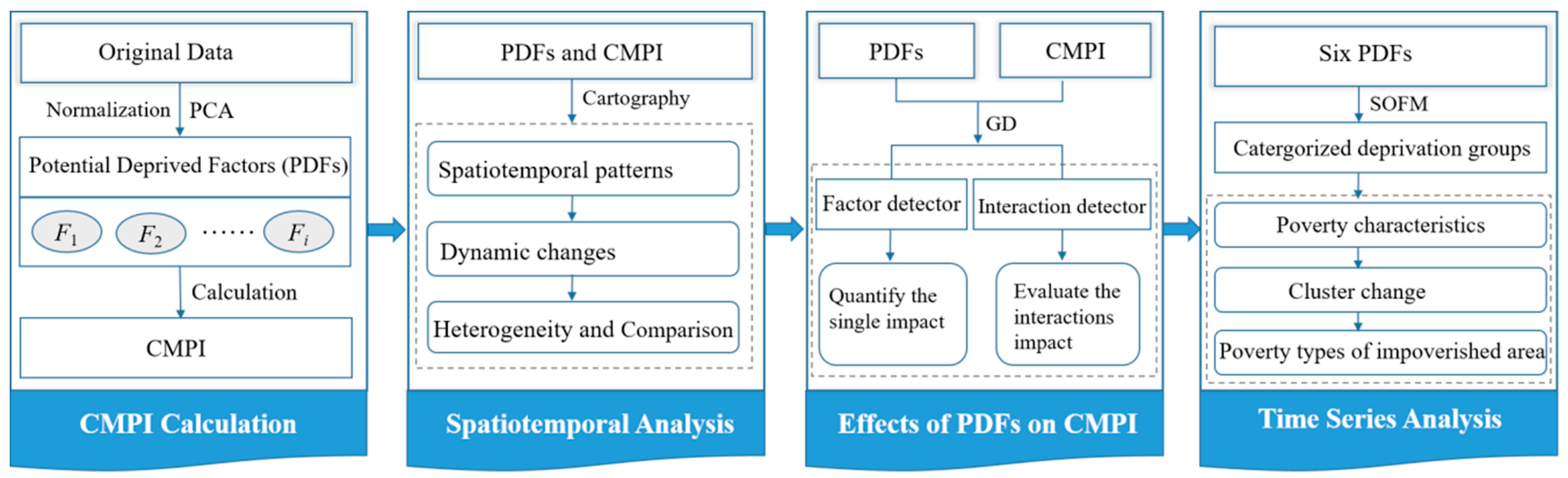
Various multidimensional poverty indices and their measures have been proposed over the past few decades. For example, the Human Development Index (HDI) was proposed by the UN Development Program in 1981 to measure well-being from three dimensions [24]. Hagenaars [25] first described multidimensional poverty from the dimensions of income and leisure. Ma and Wang [26] proposed a concept of Complex Socio-Economic-Natural Ecosystems (CSENE) to describe the relationship between human beings, society, and nature. The Oxford Poverty and Human Development Initiative proposed the Multidimensional Poverty Index (MPI) in 2010 to evaluate poverty through education, health, and living standards [23]. Alkire and Foster [27] summarized poverty from a multidimensional perspective with their widely used A-F model. The Sustainable Livelihoods Framework (SLF), established by the British Department for International Development in 2000, consists of five livelihood capitals: natural capital, social capital, human capital, physical capital, and financial capital. It has been widely adopted and applied in measuring multidimensional poverty to achieve a deeper and more complete understanding of poverty [28].

The assessment of multidimensional poverty often involves two key issues: one is the selection of poverty dimensions and variables, and the other is the calculation of the weight of indicators. Although there are many ways to measure multidimensional poverty, no consensus has been granted on the method of identifying and measuring poverty indicators because the results from different study areas and research perspectives are often different. In addition, the two most commonly used methods for calculating poverty indicators are fixing a weighting scheme and setting a deprivation threshold. For example, determining whether a household or region is poor by summing each weighted degree, or setting a deprivation threshold below which it is considered to be poor. However, these calculation methods are too subjective with potential bias and uncertainty [18]. Few current studies have considered data-driven approaches to address underlying poverty factors and find the best comprehensive variable combination for poverty estimation.

3. Data and Method

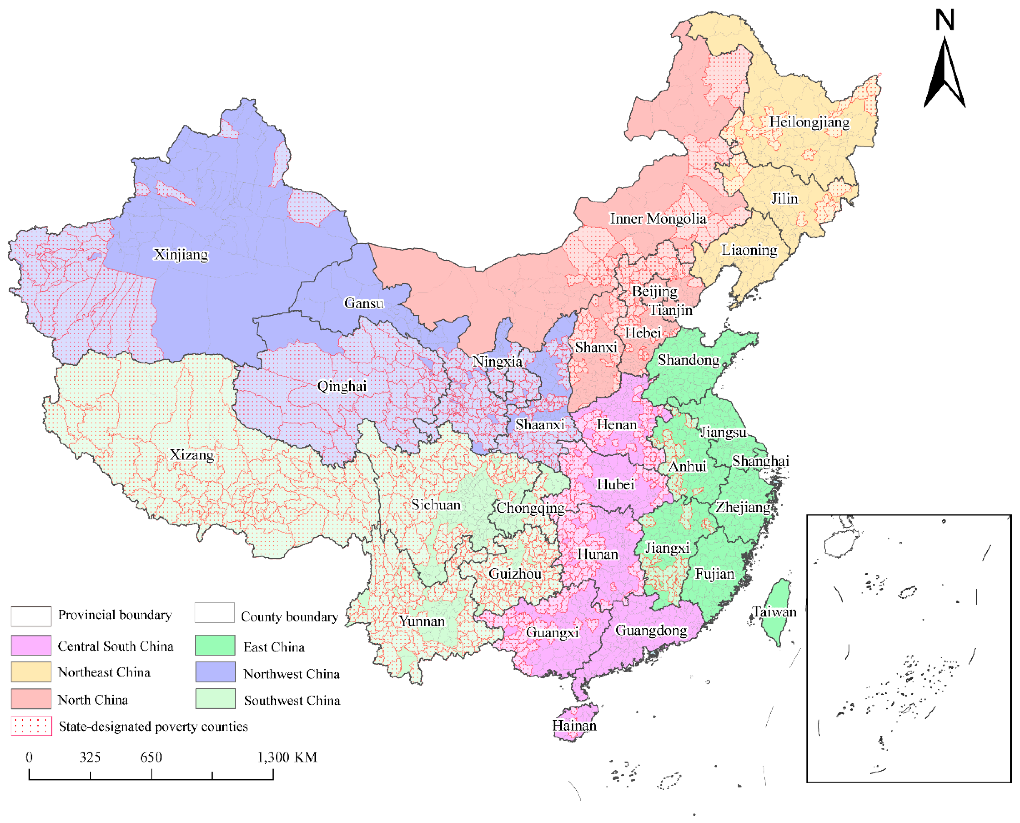
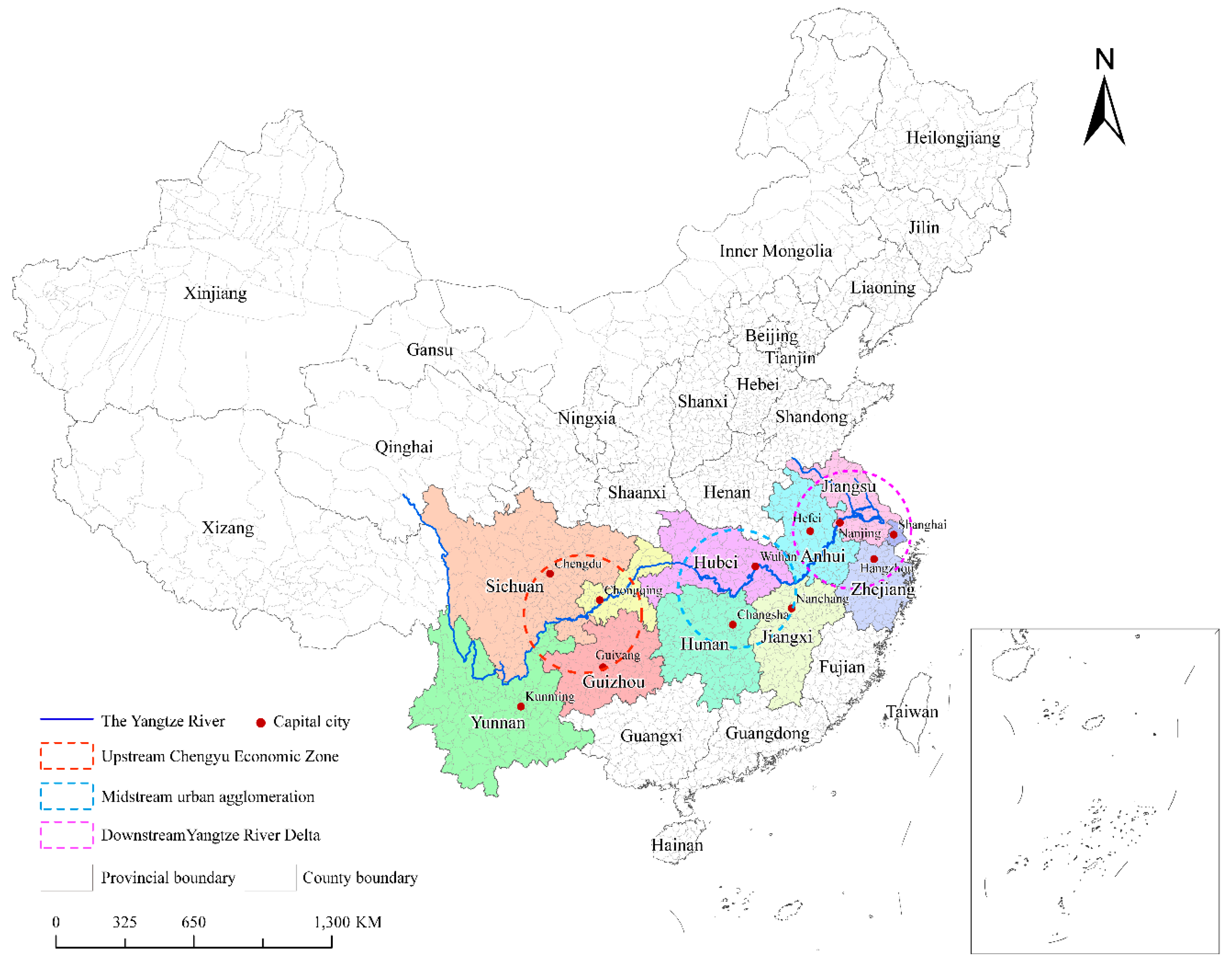
3.1. Study Area and Data

China has six main regions: Northeast, North China, East China, South Central, Northwest, and Southwest. Counties are the basic local administration units in China, with a total of 2851, including 832 state-designated poverty counties (Figure 1). Most of the state-designated poverty counties are clustered in old revolutionary base areas, ethnic minority areas, and frontier areas, and are the key areas for China’s poverty alleviation program. This study was conducted at the county level to establish a poverty index for the entire country as sub-county census statistics are not reported. This study area includes 2022 counties in mainland China, with 771 state-designated poverty counties and 1251 non-state-designated poverty counties.

We selected 26 indicators covering 5 livelihood capital and vulnerability environment variables according to SLF, CSENE, and the other related literature.

Table 2. The taxonomy and description of selected indicators at the county level.

Dimensions	Variables	Indicators	Explanation and Calculation Process	Select Basis and References
Nature	Topographical factors	X1: Average altitude	Meters above sea level (m)	High-altitude areas in China are mostly remote mountainous areas, with inconvenient transportation and underdeveloped economies [12]. The level of poverty is relatively high.
		X2: Topographic relief	Difference between the highest altitude and the lowest altitude of the county (m)	Complicated topographical conditions have a strong positive driving effect on the spatial distribution of poor counties [29].
	Meteorological factors	X3: Annual average precipitation	Annual average precipitation at county level (mm)	In arid areas with low annual precipitation, industrial and agricultural production and operation activities are more restricted by water resources [29].
		X4: Annual temperature	Annual average temperature at county level (℃)	Generally speaking, good climate conditions are favorable for both residents’ life and their crop production [30].
Human	Population conditions	X5: Non-agricultural population	Percentage of non-agricultural population (%)	Human resources are the first element of economic society. The urban population of a region is often positively correlated with the economic growth rate [31].
		X6: Rural population	Percentage of rural population (%)	China has a rural population of more than 800 million. Many agricultural populations are mainly engaged in low-income physical labor. In theory, areas with higher rural populations are poorer [31].
	Labor factors	X7: Employees	Ratio of employees to the total population at year-end (%)	Increased employment opportunities will lead to increased incomes and thus alleviate poverty [30].
		X8: Rural labor force	Ratio of rural force to rural population (%)	Rural labor is the basic factor of agricultural production and plays an important role in the rural economy [32].
Society	Social security	X9: Medical condition	Number of beds in hospitals and health centers owned per 10,000 people	In poverty-stricken areas, the phenomena of disease-caused poverty and returning-to-poverty are prevalent [33]. The better the medical conditions in a region, the lower the poverty rate.
		X10: Social welfare condition	Number of beds in social-welfare institutions owned per 10,000 people	The number of beds in social welfare institutions is usually regarded as one of the poverty indicators of social security [30]. The better the social welfare system in a region, the lower the poverty rate.
		X11: Compulsory education condition	Ratio of number of primary and secondary school students to the total population in a county (%)	Education will relatively affect the conversion of traditional poverty to non-poverty [32].
Material	Agricultural productions	X12: Farmland production potential	Potential productivity of farmland at county level (kg/ha)	The production potential of farmland reflects the arable level of the countryside, which is closely related to the livelihood of farmers [34]).
		X13: Agricultural mechanization investment	Total agricultural machinery power at county level (104 kW)	Agricultural mechanization is conducive to reducing crop rotation and thus promoting grain production. It will increase the income level of famers in rural areas [31].
	Grain factors	X14: Per capita grain output	Ratio of total grain output to total population in a county (kg per person)	Grain and poverty are often closely related. To solve the root causes of rural poverty, we must solve the problems that relying on grain creates. It is also a prerequisite for rural development [35].
		X15: Ratio of grain crops	Proportion of grain crop yield to crop yield (%)	The higher the ratio of grain yield to crop yield in the region, the better the agricultural production. However, the economic level of regions generally dominated by agriculture is low [34].
		X16: Ratio of economical crop yield	Proportion of economical yield (cotton, oil, and meat) to crop yield (%)	In theory, the higher the proportion of economical yield, the richer the crop structure and the better the economic level of the region [34].
Economy	Industrial conditions	X17: Industrial advantage	Number of industrial enterprises above designated size	Industrial enterprises above a designated size in China refer to those whose annual main business income is more than CNY 20 million. The higher the number means the higher the degree of local industrialization and urbanization [30].
		X18: Industrial output value	Gross industrial output value above designated size (CNY)	A high industrial output value means that more employment opportunities can be provided, which is conducive to poverty alleviation [30].
		X19: Capital construction	Capital construction investment completed (CNY)	The completed capital construction investment represents the actual level of industrial development [31].
	Income factors	X20: Per capita GDP	Ratio of gross domestic product (GDP) to total population at county level (CNY per person)	GDP is often recognized as the best indicator of the economic conditions of a country or region. It reflects the economic strength and market size of a region [12].
		X21: Financial situation of government	Ratio of public expenditure to income (%)	The ratio of public expenditure to income can directly reflect the financial level of a region. The lower the ratio, the better the economy [35].
		X22: Economic status of residents	Per capita savings deposit balance of urban and rural residents at year-end (CNY)	Savings are the surplus of people’s income, which can reflect their living and income levels [32].
	Industrial structure	X23: Ratio of agricultural added value	Proportion of value added of the primary industry accounts for the regional GDP (%)	Primary industry mainly includes forestry, animal husbandry, fishery, etc. A higher ratio means that the region focuses on agriculture and has lower local economic development [35].
		X24: Ratio of manufacturing added value	Proportion of value added of the secondary industry (manufacturing and industrial sector) accounts for the regional GDP (%)	The added value of secondary industry is an important index for measuring the industrial structure. The higher the ratio, the richer the industrial structure [35].
Environmental vulnerability		X25: Ratio of slope above 15°	Proportion of slope area above 15° (%)	Areas with higher slopes and greater terrain undulations have harsher land use conditions and more difficult farming and traffic conditions. This is usually regarded as one of the indicators of environmental vulnerability [36].
		X26: Annual vegetation coverage	NDVI value at county level	NDVI can reflect the vulnerability of the ecological environment, which is closely related to poverty [30].

presents the description, calculation process, and selection basis of all indicators used in this paper. We collected raw data from the following sources to calculate the indicators:

Digital elevation models (DEMs): The DEM of the whole study area was provided by the NASA Shuttle Radar Terrain Mission (SRTM) (http://www.gscloud.cn, accessed on 16 January 2022), with a resolution of 90 m.

Meteorological data:The annual average temperature and annual precipitation data were from daily observations of more than 2400 meteorological stations in China. These source data were provided by the Data Center for Resources and Environmental Sciences (RESDC), Chinese Academy of Sciences (http://www.resdc.cn, accessed on 16 January 2022).

Normalized Difference Vegetation Index (NDVI):The annual vegetation index data were generated by the maximum value synthesis method based on the monthly data of MODIS/Terra MOD13A2 product (https://lpdaac.usgs.gov, accessed on 16 January 2022).

Farmland production potential data: This index used the Global Agro-Ecological Zones model to estimate the production potential of China’s cultivated land acquired based on the data of arable land distribution, soil, and elevation. In the process of estimating grain production potential, five major grain crops—wheat, corn, rice, soybean, and sweet potato—were mainly considered, accounting for 97.7% of China’s total grain output. The dataset was processed and provided by the RESDC. We extracted and calculated the total grain yield of each county from the dataset.

Population, labor, and social–economic statistics These data were collected from the China County Statistical Yearbook from 2000 to 2015 (http://www.yearbookchina.com/index.aspx, accessed on 16 January 2022). All data were processed and calculated on the county level.

County-level administrative divisions The data were obtained from the Geographical Information Monitoring Cloud Platform (http://www.dsac.cn/, accessed on 16 January 2022).

3.2. Methods

Figure 2 shows the overall methodological framework with four main steps. Firstly, the potential deprivation factors (PDFs) were found from 26 variables with principal component analysis (PCA), and then a comprehensive multidimensional poverty index (CMPI) was calculated. The purpose of this is to automatically obtain the optimal combination of poverty deprivation variables based on a data-driven approach, thereby avoiding the interference of subjective selection, calculation bias, and overlap of independent variables. Secondly, visual analysis was applied to reveal the spatiotemporal patterns, dynamic changes, and heterogeneity of multidimensional poverty in China. The spatiotemporal dynamics and characteristics of multidimensional poverty can be better described through cross-temporal analysis, which contributes to the interpretability and accuracy of the results at the spatiotemporal and regional scales. Thirdly, we quantified the impact of the PDFs on the CMPI by using the geographical detector (GD) method and revealed interactions between PDFs. Lastly, we analyzed the characteristics and causes of multidimensional poverty in counties using Self-Organizing Feature Mapping (SOFM). By aggregating the six PDFs in one space, the characteristics, causes, and changes of poverty in different counties on spatiotemporal scales can be further revealed. The following sections explain these steps in detail.

3.2.1. CMPI Calculation

Before modeling, all indicators are normalized by Zero-mean Normalization to make the data normally distributed in order to reduce heteroscedasticity [37]. The mean value of the standardized data is 0 and the standard deviation is 1. It can give different features the same scale, which is conducive to the reliability of the results. Suppose there are m evaluating objects and n indicators. The indicators value matrix can then be formed as:

$$X=\left[\begin{array}{cccc}x11& x12& \cdots & x1n\\ x21& x22& \cdots & x2n\\ ⋮& ⋮& ⋮& ⋮\\ xm1& xm2& \cdots & xmn\end{array}\right]=\left\{X_{ij}\right\}{}_{m\times n} \left(1\le i\le m,1\le j\le n\right)$$

(1)

where X is the matrix of sample observation, m is the total number of counties, and each county has poverty measure values of n dimensions.

$$X_{ij}^{*}=\frac{X_{ij}-\mu }{\sigma }$$

(2)

where $\sigma =\sqrt{\frac{{\displaystyle {\sum }_{i=1,j=1}^N{(X_{ij}-u)}^2}}{N}}$; X_ij represents the value of indicator i for county j; N is the number of samples for each feature; μ is the mean value of indicator i; and σ is the standard deviation of indicator i for all counties, respectively.

This study performed PCA on the selected 26 indicators to obtain the PDFs. The CMPI was then calculated based on the PDFs. The comprehensive multidimensional poverty index of county t (CMPI_t) is formulated as:

$${\mathrm{CMPI}}_t={\displaystyle \sum }_{k=1}^p{\lambda }_k\times F_i^{*}={\displaystyle \sum }_{k=1}^p{\lambda }_k\times \left({\displaystyle \sum }_{m=1}^n{L}_j\times X_j^{*}\right)$$

(3)

where ${\lambda }_k$ represents the weight of component k; p is the number of principal components; $F_i$ is the i^th PDF; $L_j$ is the loading score coefficient of indicator j; $X_j^{*}$ is the standardized value of indicator j; and n is the total number of observations.

To better interpret the results and eliminate the negative values in the results, we used $F_i^{*}=\frac{\max Fi-Fi}{\max Fi-\min Fi}$ to a negative factor and $F_i^{*}=\frac{Fi-\min Fi}{\max Fi-\min Fi}$ to a positive factor for further data processing of each PDF F_i. The processed PDFs are thus all positive values, and the higher the value, the higher the multidimensional poverty.

3.2.2. Geographical Detector (GD)

Geographical detector (GD) is a tool for detecting and exploring spatial heterogeneity. Compared to the traditional regression model, it has the advantage of not relying on any assumptions, such as the uniformity of variance or independent errors [38]. This study used GD to quantify the driving mechanisms of the CMPI and reveal the interactions among the PDFs. Therefore, two functions of GD are used to analyze the relationship and interaction among the PDFs.

1.

Factor detector (FD) is used to quantify how much a factor can explain the spatial differentiation of the CMPI. It is usually measured by the q-statistic [39], as shown in Formula (4):

$$Q_{(F_i,C)}=1-\frac{1}{N{\sigma }_C^2}{\displaystyle \sum _{m=1}^n{N}_{(F_i,m)}^{’}}{\sigma }_{C(F_i,m)}^2$$

(4)

where N is the total number of counties in this study;$N_{(F_i,m)}^{’}$ is the county in the m^th parcel of F_i; n is the total number of parcels for F_i; and ${\sigma }_C^2$ and ${\sigma }_{C(Fi,m)}^2$ represent the variance of the CMPI for the whole study area and in the m^th parcel, respectively. The value of $Q_{(F_i,C)}$ is within [0, 1], which reflects the influence of F_i on the CMPI. A larger q-statistic value indicates a stronger impact of a PDF F_i on the CMPI.

2.

Interaction detector (ID) identifies the interactive effect on the CMPI between different factors to evaluate whether the interaction of the PDFs will increase or decrease the explanatory power of the CMPI. The relationship can be divided into five categories.

Table 3. Descriptions and interaction relationships.

Description	Result Representation	Interaction Relationship
q(x1∩x2) < Min(q(x1), q(x2))		Weakened, nonlinear
Min(q(x1), q(x2)) < q(x1∩x2) < Max(q(x1), q(x2))		Weakened, univariate and nonlinear
q(x1∩x2) > Max(q(x1), q(x2))		Enhanced, bivariate
q(x1∩x2) = q(x1) + q(x2)		Independent
q(x1∩x2) > q(x1) + q(x2)		Enhanced, nonlinear

Note: Min(q(x₁), q(x₂)) Max(q(x₁), q(x₂)) q(x₁) + q(x₂) q(x₁∩x₂).

shows their description and interaction relationship.

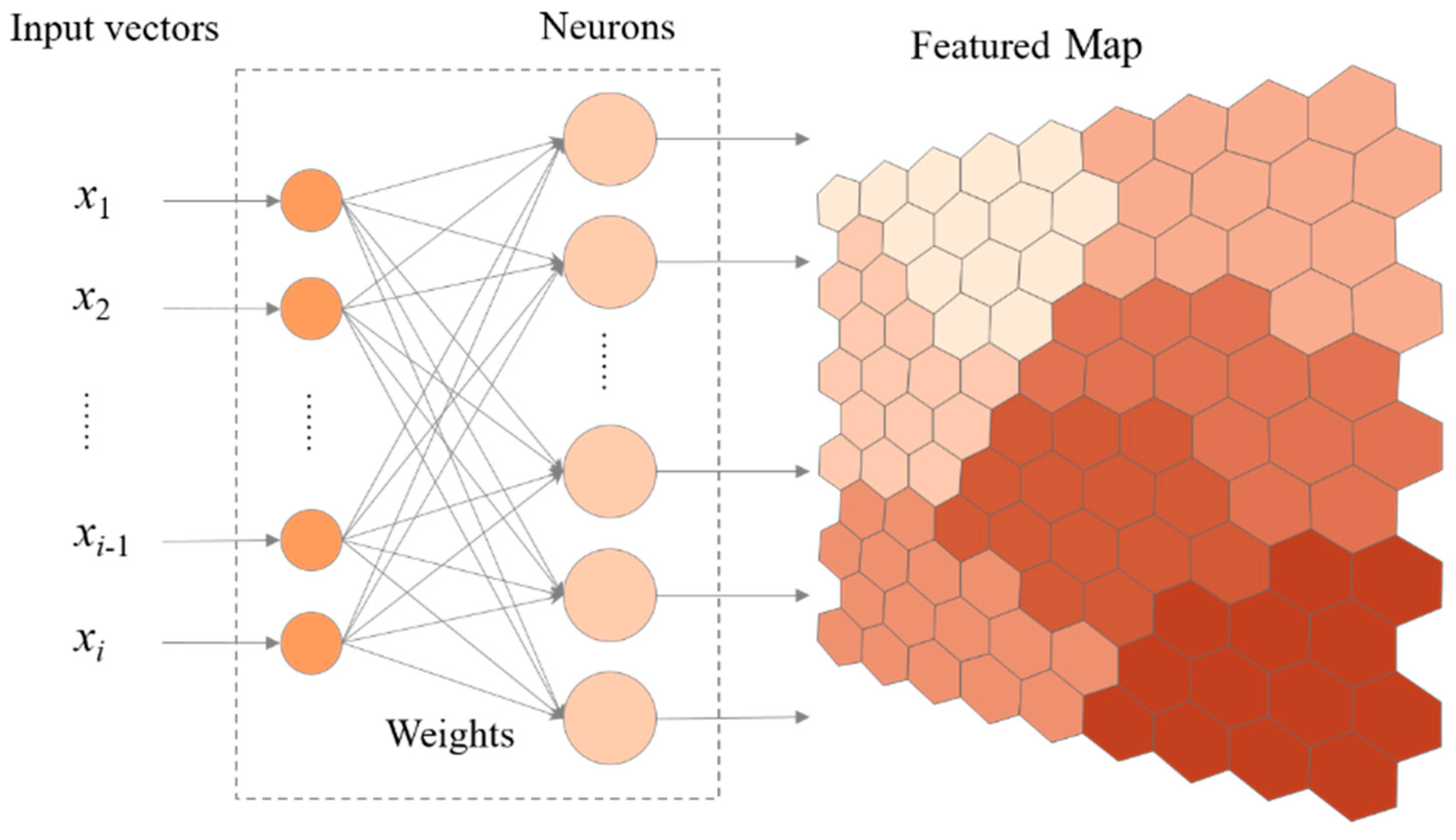
3.2.3. Self-Organizing Feature Mapping (SOFM)

Self-Organizing Feature Mapping (SOFM) is one of the most widely used neural networks for dimensionality reduction [40]. As an unsupervised computational neural network, SOFM can process highly nonlinear and high-dimensional data and simplify the input layer into a low-dimensional regular array [41], as shown in Figure 3. Compared to traditional clustering methods, SOFM has three significant advantages: no prior knowledge requirements, the ability to handle nonlinearities, and the applicability of visualization [42]. The workflow of SOFM is as follows:

First, the Euclidean distance between the input sample X and each output neuron j is calculated. W_ij is the weight between the i^th neuron of the input layer and the j^th neuron of the mapping layer.

$$d_j=\parallel X-W_j\parallel =\sqrt{{\displaystyle \sum _{i=1}^m{(x_i(t)-{\omega }_{ij}(t))}^2}}$$

(5)

Second, the weights of output neuron j* and its neighboring neurons are modified, where $\eta (t)=\frac{1}{t}$ is a constant and gradually decreases to 0 along time.

$${\omega }_{ij}(t+1)-{\omega }_{ij}(t)=\eta (t)\left[x_i(t)-{\omega }_{ij}(t)\right]$$

(6)

Last, the output O_k is calculated. If it meets the requirements (Formula 7, neuron j with the smallest distance obtained), the algorithm ends; otherwise, it returns to the next round of learning.

$$O_k=f(\underset{j}{\min }dj)=f(\underset{j}{\min }\parallel X-Wj\parallel )$$

(7)

This paper employs SOFM to classify the PDFs’ typology for revealing the multidimensional poverty dynamics across time and drawing their spatial agglomerations. We trained a self-organizing neural network with 2022 counties as geographic samples and the PDFs as sample features to define spatial clustering.

4. Results

4.1. PDFs and CMPI

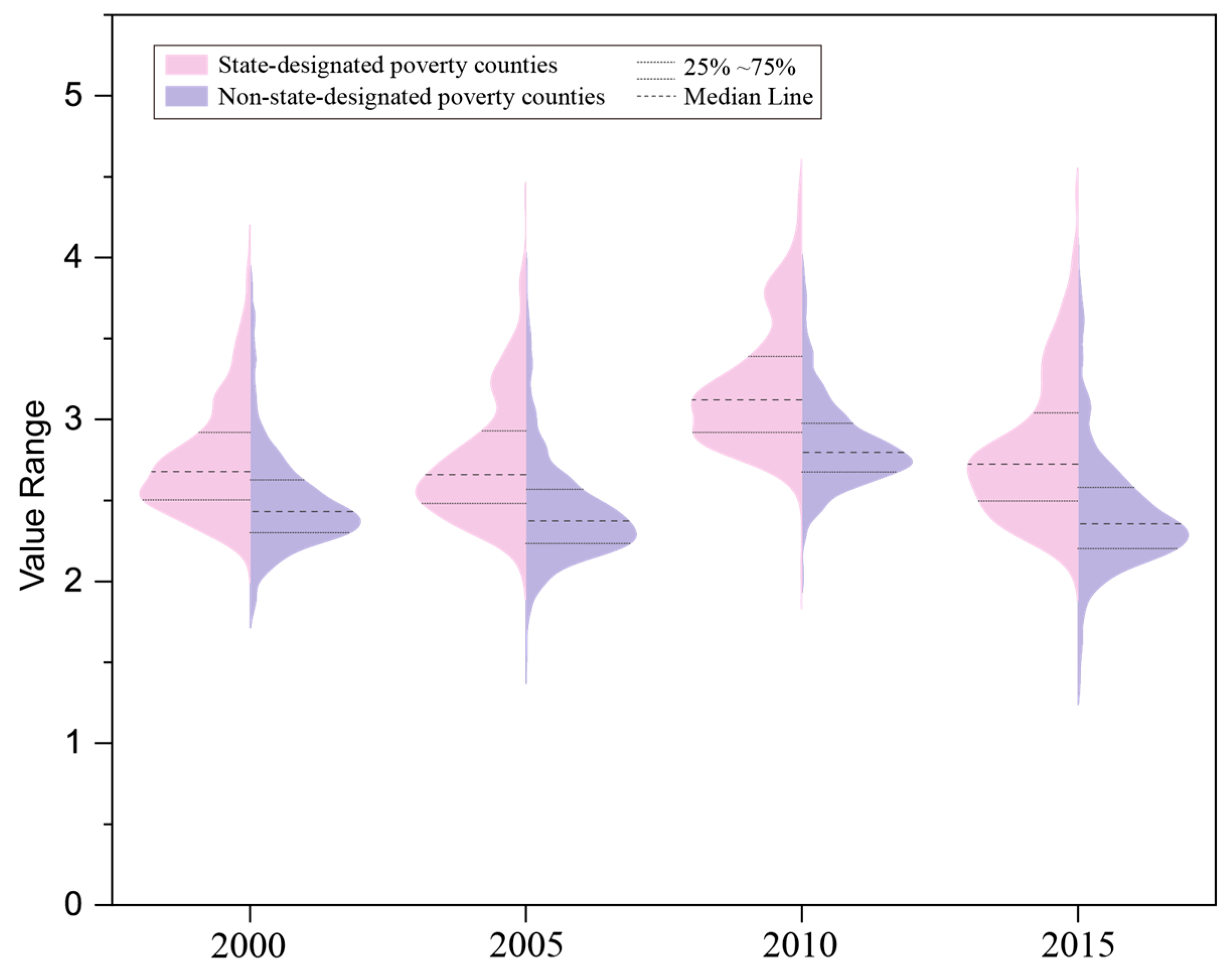
4.1.1. The General Description

Table 4. Total variance and components extracted by the varimax rotating PCA.

Components	Eigenvalue	% of Variance	Cumulative%
1	6.984	24.942	24.942
2	4.898	17.495	42.437
3	3.279	11.709	54.146
4	2.628	9.387	63.534
5	2.458	8.779	72.313
6	2.000	7.142	79.456

describes six principal components (PCs) generated by PCA, explaining approximately 80% of the total variance.

Table 5. Formulation of the CMPI and the six PDFs.

Domain	Value	Range	Mean	Std.
Economic capital deprivation (F1)	F1 = 0.240 × X17 + 0.265 × X18 + 0.230 × X19 + 0.182 × X0 + 0.169 × X22	(0,1)	0.934	0.080
Geographical capital deprivation (F2)	F2 = 0.187 × X1 + 0.228 × X2 + 0.293 × X25	(0,1)	0.245	0.210
Natural resource endowment capital deprivation (F3)	F3 = 0.330 × X3 + 0.316 × X4 + 0.260 × X26	(0,1)	0.439	0.195
Agricultural capital deprivation (F4)	F4 = 0.245 × X12 + 0.221 × X13 + 0.443 × X15 − 0.442 × X16	(0,1)	0.212	0.132
Human and labor capital deprivation (F5)	F5 = −0.469 × X5 + 0.468 × X6 − 0.408 × X7	(0,1)	0.627	0.229
Compulsory education deprivation (F6)	F6 = −0.590 × X11	(0,1)	0.220	0.106
Comprehensive multidimensional poverty index (CMPI)	CMPI = F1 + F2 + F3 + F4 + F5 + F6	(0,5)	2.677	0.430

lists six PDFs and the final CMPI calculated using Equations (2) and (3) to evaluate the multidimensional poverty status in China in six aspects from 2000 to 2015. Among them, PC 1 (F₁) includes five high loading economic factors, indicating the disadvantaged economic capital. PC 2 (F₂) contains three high load geographic factors, representing poverty caused by geographic capital deprivation. Similarly, the other four components represent natural resource endowment capital deprivation (F₃), agricultural capital deprivation (F₄), human and labor capital deprivation (F₅), and compulsory education deprivation (F₆). The factor loadings of the 26 input indicators in the varimax rotated matrix for the six retained PCs are shown in Appendix B (

Table A1. The factor load of input indicators calculated by PCA. Indicators with numbers in bold are high loading factors for each PC.

Indicators	Main Principal Components
	PC 1	PC 2	PC 3	PC 4	PC 5	PC 6
X1: Altitude	−0.193	0.670	−0.596	−0.091	0.021	0.002
X2: Topographic relief	−0.151	0.740	−0.338	−0.066	−0.043	0.041
X3: Annual average precipitation	0.036	0.236	0.827	0.002	0.139	0.093
X4: Annual temperature	0.127	−0.073	0.848	0.019	0.174	−0.176
X5: Non-agricultural population	−0.057	0.008	−0.113	−0.081	−0.945	0.072
X6: Rural population	−0.056	−0.008	0.113	0.081	0.946	−0.072
X7: Employees	0.284	0.058	−0.021	−0.032	−0.656	−0.044
X8: Rural labor force	0.265	0.018	0.202	0.004	−0.118	0.183
X9: Medical condition	0.289	0.175	−0.170	−0.104	−0.312	−0.107
X10: Social welfare condition	0.143	−0.133	0.134	−0.024	0.121	0.450
X11: Compulsory education condition	−0.026	0.024	−0.019	0.018	0.144	−0.729
X12: Farmland production potential	−0.039	−0.777	−0.085	0.777	−0.006	0.258
X13: Agricultural mechanization investment	0.188	−0.705	−0.027	0.705	0.123	0.002
X14: Per capita grain output	−0.116	−0.498	−0.247	0.522	−0.017	0.273
X15: Ratio of grain crops	0.014	−0.033	0.138	0.959	0.095	−0.049
X16: Ratio of economical crop yield	−0.012	0.035	−0.142	−0.958	−0.086	0.049
X17: Industrial advantage	0.787	−0.115	0.110	−0.074	0.174	0.181
X18: Industrial output value	0.849	−0.125	0.032	−0.071	0.127	0.123
X19: Capital construction	0.764	−0.212	0.050	−0.021	0.037	0.108
X20: Per capita GDP	0.721	−0.096	−0.090	−0.075	−0.020	−0.019
X21: Financial situation of the government	−0.270	0.298	−0.419	−0.067	0.081	0.154
X22: Economic status of residents	0.737	−0.057	0.028	−0.096	−0.115	−0.057
X23: Ratio of agricultural added value	−0.529	−0.018	−0.057	−0.159	0.059	0.268
X24: Ratio of manufacturing added value	0.350	−0.034	0.094	0.112	−0.013	−0.077
X25: Slope ratio over 15°	−0.206	0.857	0.069	0.074	0.084	0.114
X26: Annual vegetation coverage	−0.103	−0.136	0.684	0.245	0.045	0.305

Note: Based on Wan and Su (2017), we only kept indicators with a high loading value (≥0.65) for each PC.

). All the PCs cover the five dimensions of the Sustainable Livelihoods Framework and reflect the state of multidimensional poverty from different aspects, demonstrating the strength and effectiveness of PCA in formulating the CMPI.

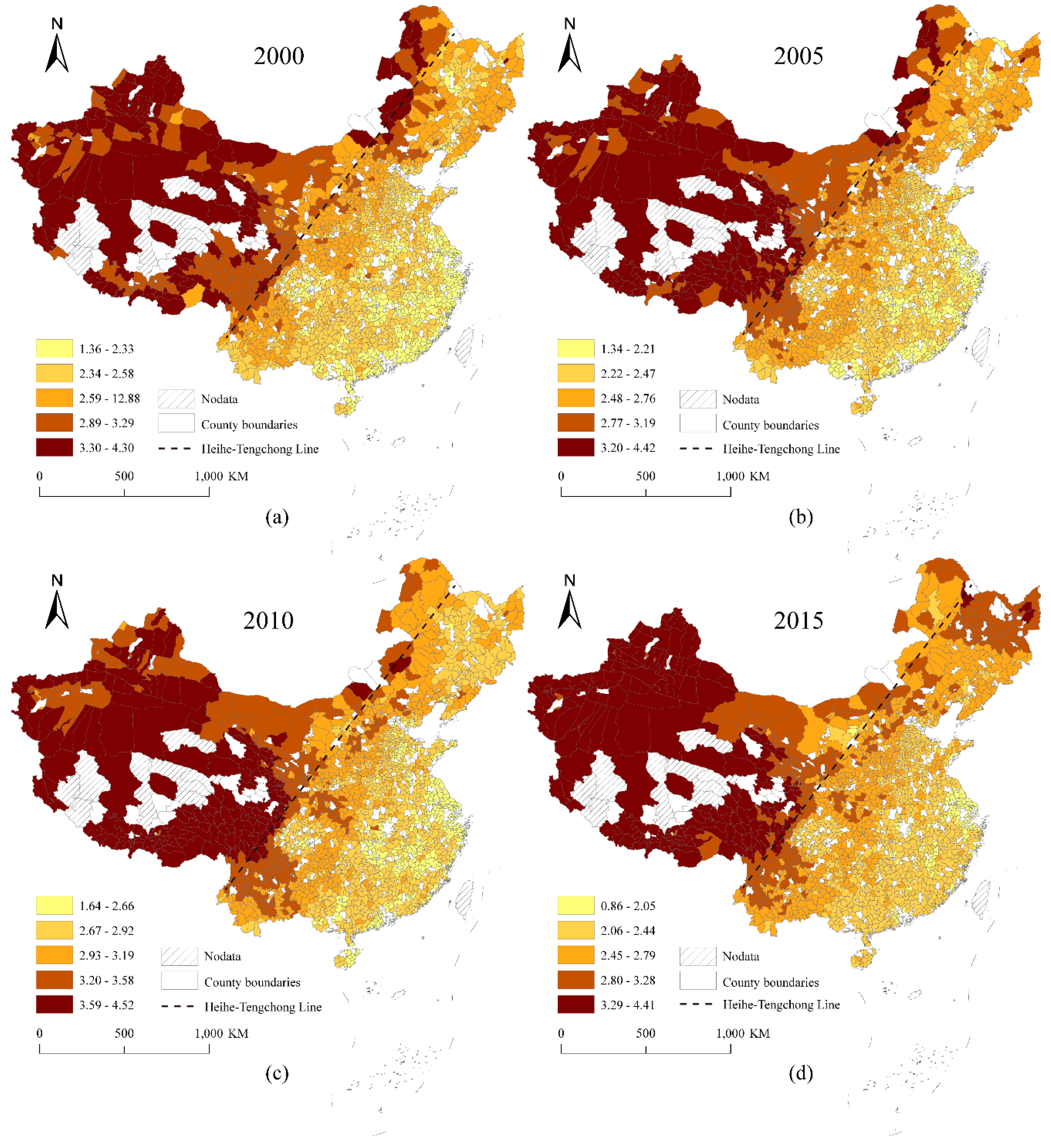
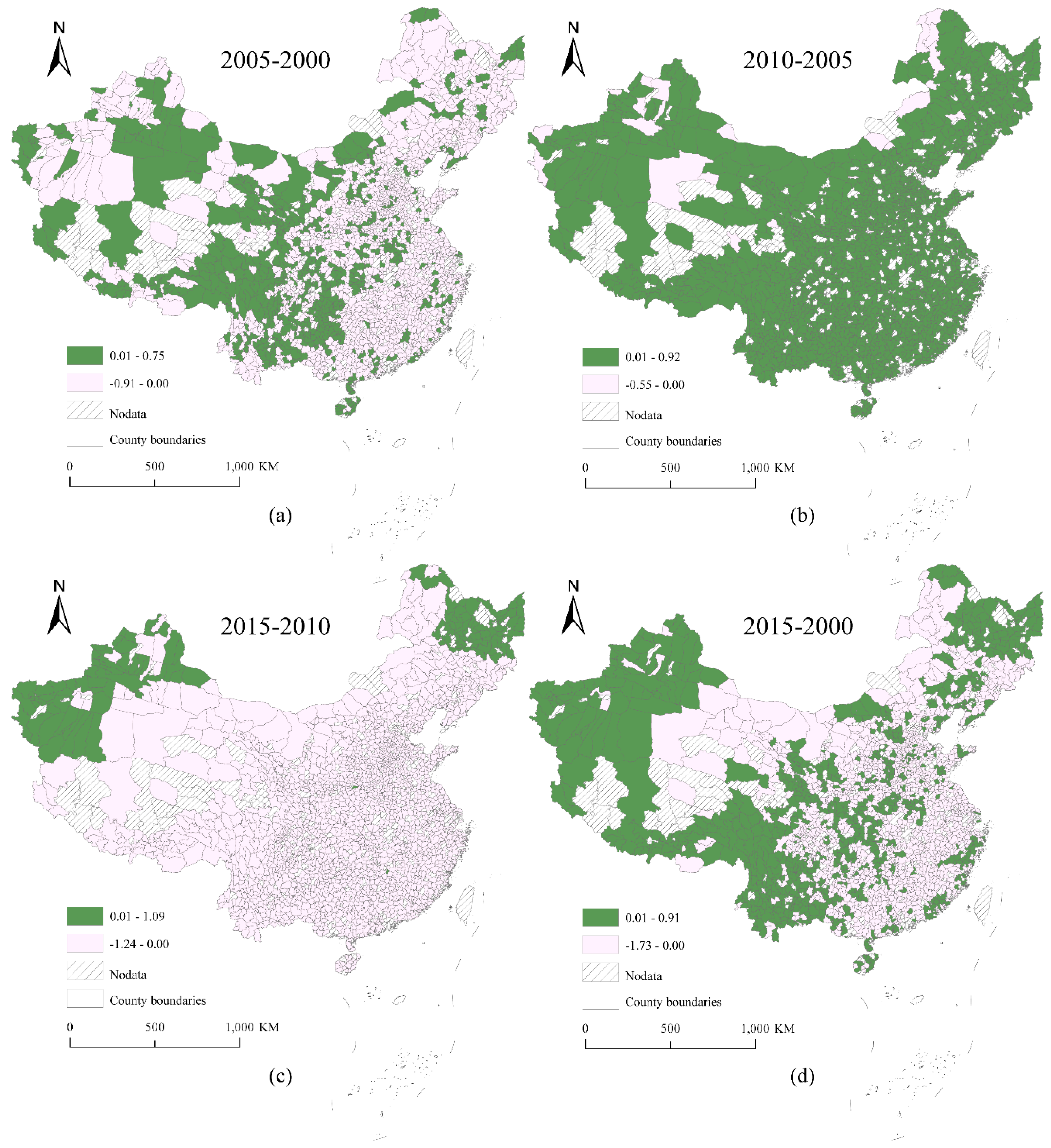
4.1.2. Spatiotemporal Patterns and Dynamic Changes

The spatial distribution of the CMPI varies over time at the county level (Figure 4). In general, counties with lower CMPI values are located along the eastern coast of China, while those with higher CMPI values are distributed in the Northwest, Southwest, and north of Northern China, mainly concentrated in areas of the Tibet autonomous region, three prefectures in Southern Xinjiang, Tibetan areas in four provinces, Liupan Mountains, Yanshan–Taihang Mountains, Western Yunnan border mountains, etc. (Appendix A, Figure A1). Figure 5 further reveals the spatiotemporal dynamics of the CMPI. Almost a third, 33.23% (672/2022), of China’s counties experienced an increase in multidimensional poverty in 2005. The multidimensional poverty in 98.36% of areas (1989/2022) continued to worsen in 2010, while, in 2015, it showed significant improvement, with 93.76% of areas (1896/2022) alleviating multidimensional poverty. Although nearly 60% (1200/2022) of the counties have been relieved during the past 15 years (Figure 5d), the multidimensional poverty in some areas continues to deteriorate, mainly in Xinjiang, Heilongjiang, Tibet, Yunnan-Guizhou Plateau, and some counties along the southeast coast.

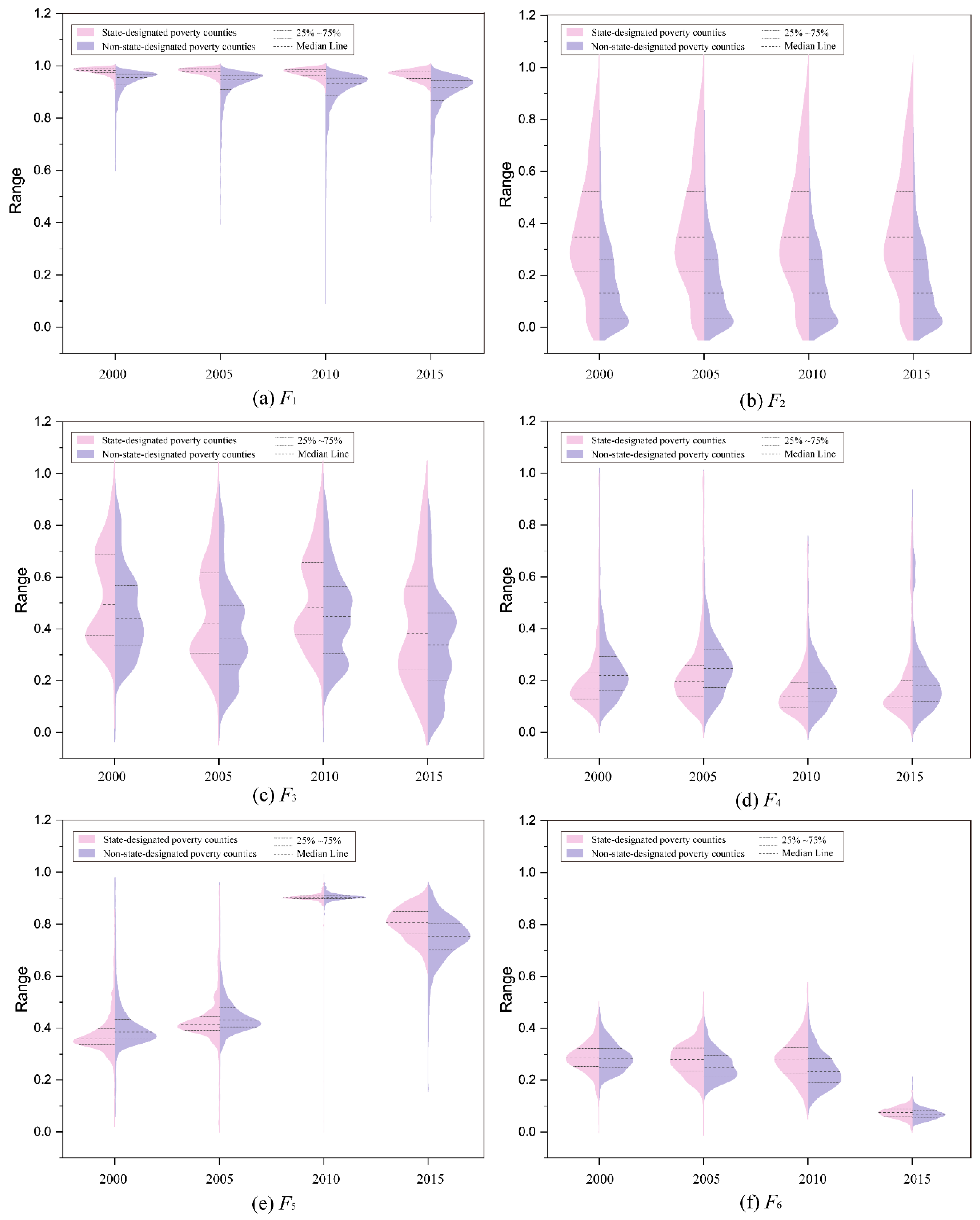
4.1.3. Heterogeneity and Comparison

To further investigate the heterogeneity of the PDFs and the CMPI, this study used violin plots to establish baseline images by block group for both state-designated poverty counties and non-state-designated poverty counties (Figure 6 and Figure 7). Figure 6 shows that the 6 PDFs have changed significantly in both levels and distributions over 15 years. Compared to the non-state-designated poverty counties, the state-designated poverty counties have poorer economic conditions and are also at a significant disadvantage in terms of geographical conditions and natural ecology. This is reflected in the fact that the medians and data concentration intervals of these three factors in poverty counties are significantly higher than those in non-poverty counties. For agricultural capital deprivation (F₄), the median line of state-designated poverty counties is lower than that of non-state-designated poverty counties, revealing that poor counties have a larger proportion of agriculture. The median line of human and labor capital in state-designated poverty counties in 2015 was much higher than in non-state-designated poverty counties, implying that they had more severe population outflows. In terms of educational conditions, non-state-designated poverty counties show obvious advantages. From the perspective of time, economic conditions, natural resource endowment, compulsory education, and agricultural capital have all improved, while human and labor capital have deteriorated significantly. A more concentrated numerical distribution suggests that deprivation should have a homogeneous pattern, while large fluctuations imply significant differences in resource allocation among China’s counties, indicating the rising inequality, especially in geographical capital deprivation (F₂), natural resource endowment capital deprivation (F₃), and human and labor capital deprivation (F₅).

The CMPI of both state-designated poverty counties and non-state-designated poverty counties also showed obvious spatiotemporal dynamics and differences over time (Figure 7). Although the CMPI values of the two categories first increased and then decreased with time, the CMPI of state-designated poverty counties was always higher than that of non-state-designated poverty counties. Among them, the CMPI values of state-designated poverty counties are concentrated between [2.5, 3.5], while those of non-state-designated poverty counties are concentrated between [2.3, 2.8]. Overall, the optimization of multidimensional poverty in non-state-designated poverty counties is higher than that of state-designated poverty counties, as shown by the decrease of the median line of non-poor counties and the increase of poor counties.

Table 6. Proportion of counties with increased CMPI value over time in state-designated poverty counties and non-state-designated poverty counties.

	Type	State-Designated Poverty Counties		Non-State-Designated Poverty Counties
Year		Number	Proportion (%)	Number	Proportion (%)
2005–2000		357	46.30	315	25.18
2010–2005		761	98.70	1228	98.16
2015–2010		52	6.74	74	5.92
2015–2000		448	58.11	373	29.82

further presents the changes of the CMPI in the two categories of counties. It can be seen that the increase of multidimensional poverty in state-designated poverty counties is always more significant than that in non-state-designated counties. Among them, the CMPI of 46.3% of state-designated poverty counties increased in 2005, compared to 25.18% of non-state-designated poverty counties. In 2010, more than 98% of the two types of counties showed a continuous increase in the CMPI, and both showed a decline in 2015. However, the proportion of counties with an increased CMPI in state-designated poverty counties was always higher than that in non-state-designated poverty counties, showing a higher level of poverty. Finally, in our observation period (2000–2015), the CMPI of 70.18% of non-state-designated counties decreased over time, while more than half of the state-designated poverty counties (58.11%) had their CMPI increase, indicating that the degree of multidimensional poverty in those regions is still in continuous deterioration.

4.2. Effects of PDFs on CMPI

This section focuses on analyzing the impact of each PDF on multidimensional poverty in China. Two indicators (factor detector and interaction detector) in the geographical detector (GD) are utilized to measure the interactions and relationships between the pairs of influencing factors.

4.2.1. Factor Detector (FD)

The FD quantifies the impact of the PDFs on the CMPI, exploring to what extent a factor explains the spatial differentiation of the CMPI.

Table 7. Factor detection results between the CMPI and PDFs in China’s counties. F₁ is economic capital deprivation; F₂ is geographical capital deprivation; F₃ is natural resource endowment capital deprivation; F₄ is agricultural capital deprivation; F₅ is human and labor capital deprivation; F₆ is compulsory education capital deprivation.

PDFs	2000		2005		2010		2015
	q-Statistic	p-Value	q-Statistic	p-Value	q-Statistic	p-Value	q-Statistic	p-Value
F1	0.265	0.000	0.304	0.000	0.404	0.000	0.458	0.000
F2	0.606	0.000	0.601	0.000	0.697	0.000	0.583	0.000
F3	0.497	0.000	0.467	0.000	0.370	0.000	0.489	0.000
F4	0.183	0.606	0.193	0.005	0.112	0.099	0.316	0.000
F5	0.263	0.000	0.152	0.712	0.056	0.923	0.334	0.000
F6	0.112	0.911	0.072	0.892	0.134	0.675	0.229	0.986

reveals the impacts of the PDFs based on the q-statistic. The results show that economic capital (F₁), geographical capital (F₂), and natural resource endowment (F₃) are the leading factors of multidimensional poverty. The corresponding q-statistics are relatively large and significant. This implies that the spatial differentiation of multidimensional poverty in China’s counties is significantly affected by economic capital, geographic conditions, and natural resource endowment. Furthermore, agricultural capital (F₄) and human and labor capital (F₅) are closely related to regional multidimensional poverty, but their driving force is smaller than F₁, F₂, and F₃. The q-statistic of compulsory education capital (F₆) is not statistically significant, suggesting a weak role of compulsory education in driving regional poverty, which may be related to our data: Due to the limitation of data acquisition, we only used the proportion of primary and secondary school students as the proxy for the education level of the region, without considering a series of more refined educational indicators, such as the number of universities, the number of college students, and the teacher–student ratio, which may lead to some deviation.

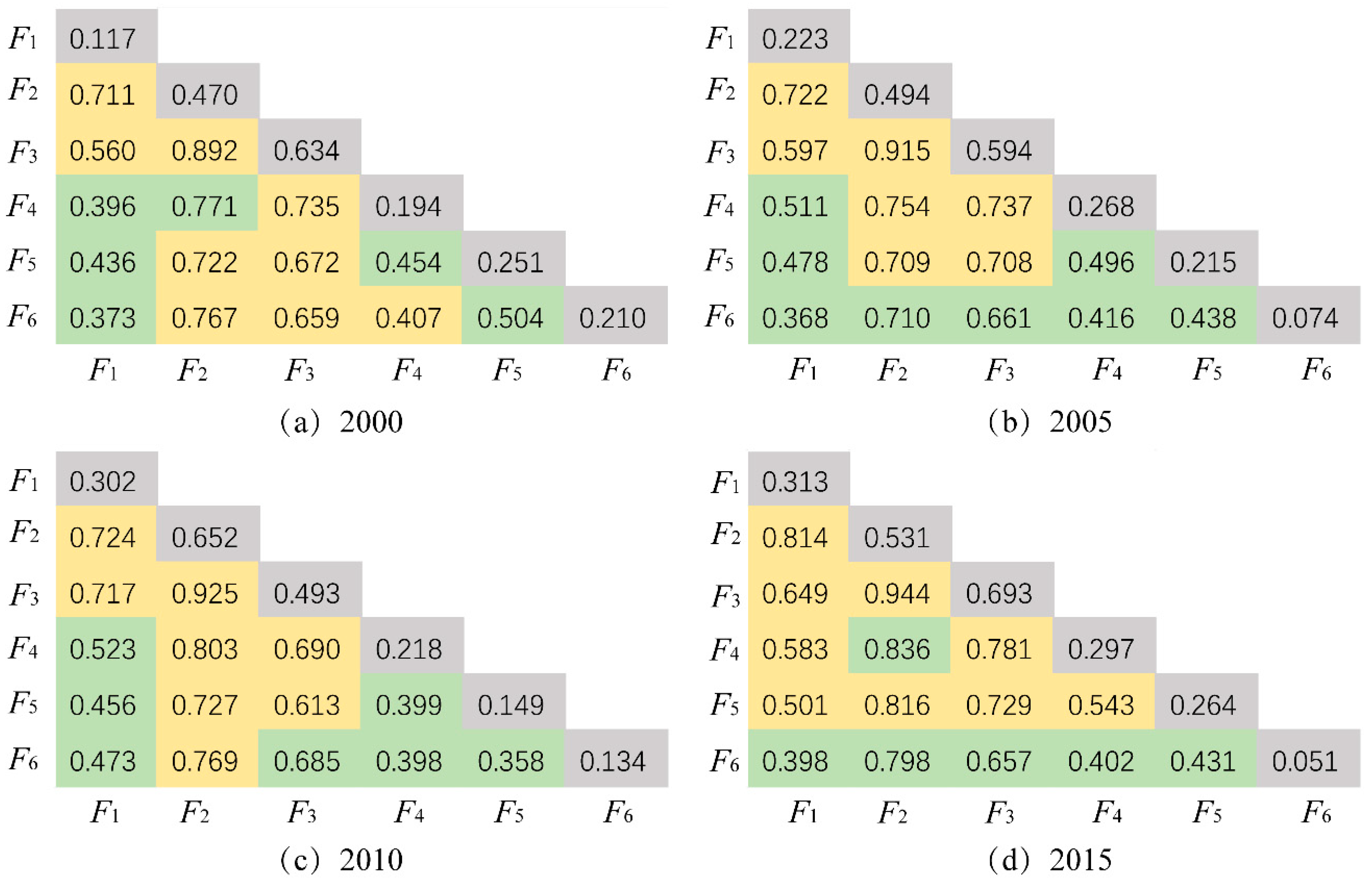
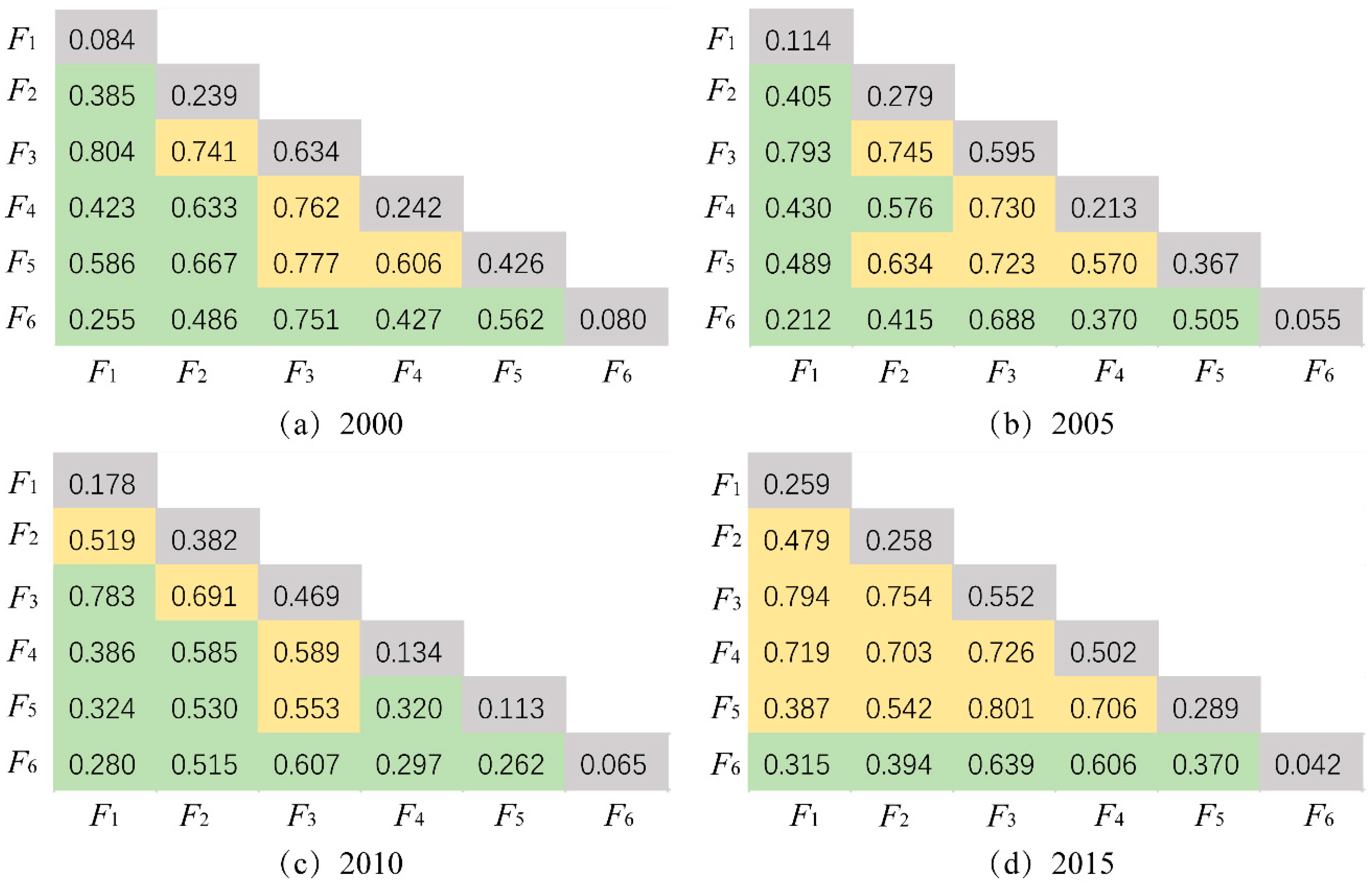
4.2.2. Interaction Detector (ID)

The ID evaluates the impact of interactions between two factors on the explanatory power of the CMPI and determines whether two factors work independently. Figure 8 and Figure 9 show the results of factor interaction detection of regional multidimensional poverty differentiation for two categories of counties. The results show that the driving force of the two-factor interaction is stronger than that of the single-factor effect, as the q-statistic of each influencing factor and other factors all increase in multiples compared to the single-factor effect. For state-designated poverty counties, the interaction relationship is dominated by bivariate enhancement (Figure 8). Geographical capital (F₂) has the strongest influence on factor interaction, with its q-statistic with other factors having increased several times compared with that alone (gray cells), and its influence having increased year by year. However, the type of factor interaction in non-state-designated poverty counties is dominated by nonlinear enhancement (Figure 9). Natural resource endowment capital (F₃) has the strongest effect on factor interaction, with the q-statistic several times higher than that of factors acting alone (gray cells). In addition, F₁ and F₃ had the largest local interaction force before 2015, while F₃ and F₅ had the strongest interaction after 2015. The results show that the combination of different PDFs had a greater impact on the CMPI than a single factor. Thus, regional poverty differentiation is the result of the combined effect of multiple factors. The multidimensional poverty pattern is affected by the synergy and long-term effects of various factors such as geographical condition, resource endowment, the economy, and population resources.

4.3. Time Series Analysis Based on SOFM

In order to further reveal the poverty characteristics and leading causes in different counties, this study divided the value of each poverty factor into three degrees according to natural break classification, including High (H), Medium (M), and Low (L) (Appendix B,

Table A2. The interval value of each PDF classified according to the natural break classification.

2000	F1	F2	F3	F4	F5	F6
High	[0.97, 1]	[0.46, 1]	[0.64, 1]	[0.43, 1]	[0.40, 1]	[0.33, 1]
Medium	[0.95, 0.97)	[0.18, 0.46)	[0.43, 0.64)	[0.22, 0.43)	[0.36, 0.40)	[0.26, 0.33)
Low	[0, 0.95)	[0, 0.18)	[0, 0.43)	[0, 0.22)	[0, 0.36)	[0, 0.26)
2005	F1	F2	F3	F4	F5	F6
High	[0.97, 1]	[0.46, 1]	[0.61, 1]	[0.44, 1]	[0.45, 1]	[0.32, 1]
Medium	[0.95, 0.97)	[0.18, 0.46)	[0.37, 0.61)	[0.23, 0.44)	[0.40, 0.45)	[0.24, 0.32)
Low	[0, 0.95)	[0, 0.18)	[0, 0.37)	[0, 0.23)	[0, 0.40)	[0, 0.24)
2010	F1	F2	F3	F4	F5	F6
High	[0.96, 1]	[0.46, 1]	[0.59, 1]	[0.37, 1]	[0.91, 1]	[0.33, 1]
Medium	[0.93, 0.96)	[0.18, 0.46)	[0.37, 0.59)	[0.17, 0.37)	[0.88, 0.91)	[0.23, 0.33)
Low	[0, 0.93)	[0, 0.18)	[0, 0.37)	[0, 0.17)	[0, 0.88)	[0, 0.23)
2015	F1	F2	F3	F4	F5	F6
High	[0.96, 1]	[0.46, 1]	[0.58, 1]	[0.44, 1]	[0.81, 1]	[0.33, 1]
Medium	[0.92, 0.96)	[0.18, 0.46)	[0.32, 0.58)	[0.18, 0.44)	[0.74, 0.81)	[0.22, 0.33)
Low	[0, 0.92)	[0, 0.18)	[0, 0.32)	[0, 0.18)	[0, 0.74)	[0, 0.22)

for classification values). We then obtained the clustering results by applying the SOFM method for different study periods (Figure 10). Based on encoded PDFs, the SOFM grouped these counties into six clusters.

The results show that six PDFs did not show significant changes in space before 2015, indicating the causes of poverty have been relatively stable for a certain period. However, there was a significant change in the clustering result of some regions after 2015, mainly located in Northwest and Northeast China and the Yangtze River Economic Belt (Appendix A, Figure A2). From 2000 to 2015, many counties experienced varying increases or decreases in some factors. However, even counties with a higher CMPI value are still at a disadvantage in certain factors.

The GD result in Section 4.2 reveals that the spatiotemporal differentiation of multidimensional poverty in Chinese counties is significantly affected by economic capital, geographical conditions, and natural resource endowment. Since F₄, F₅, and F₆ have weak effects on the CMPI, and their impacts are not significant in some years, this study mainly considers the first three strong and stable poverty-causing factors (F₁, F_2, and F₃). Combined with the SOFM clustering results in Figure 10, we further summarize the following main types of impoverished regions, as shown in

Table 8. Characteristics and distribution of different types of impoverished areas.

Types of Poverty-Stricken Areas	Performance (F1-F2-F3)	Main Features	Location	County Category
Economic-condition-constrained.	H-M-L	Poor GDP, low per capita income, and low industrial value.	Yunnan, Guizhou, Chongqing, Southern Sichuan, and Southern Shaanxi.	More than 74% are state-designated poverty counties.
Resource-abundance-constrained.	M-M-H	Low precipitation, poor climatic conditions, and low vegetation coverage.	Heilongjiang, Jilin, Shanxi, Inner Mongolia, Ningxia, Gansu, and Northern Shaanxi.	More than 52% are non-state-designated poverty counties.
Economic-condition and resource-abundance jointly constrained.	H-M-H	Low economic indicators and poor resource endowment.	Northern Xinjiang, Western Gansu, Eastern Qinghai, and some counties in Inner Mongolia.	More than 70% are state-designated poverty counties.
Economic-condition, geographic-condition, and resource-abundance cooperative constrained.	H-H-H	Low economic indicators, poor resource endowment, undulating terrain, and large slope.	Tibet, Qinghai, Northern Sichuan, and Southern Xinjiang.	More than 80% are state-designated poverty counties.
General constrained of economic-condition and geographic-condition.	M-M-L	Good resource endowment and other factors are average.	Fujian, Guangdong, Guangxi, Jiangxi, Hunan, Hainan, and Southern Zhejiang.	More than 72% are non-state-designated poverty counties.
General constrained of resource-abundance.	L-L-M	Good economic and geographical conditions, and other factors are average.	Yangtze River Delta, Hubei, Henan, Shandong, Hebei, Liaoning, and Beijing.	More than 89% are non-state-designated poverty counties.

.

From Figure 10 and Table 8, it can be seen that the economic-condition-constrained type is mainly concentrated in Southwest China, and most are state-designated poverty counties. The resource-abundance-constrained type is mainly located in most areas of the North and Northeast, while most of the Northwest area is restricted by both economic conditions and resource abundance. Many counties in Tibet, Qinghai, Xinjiang, and Sichuan are located in mountainous areas and plateaus, belonging to contiguous poverty-stricken areas. Multidimensional poverty in these regions is strongly influenced by geographical location. At the same time, it is also affected by economic conditions and natural resource abundance. The east is the concentrated area of China’s developed counties, and the six factors generally perform well, but there are still some factors that need improvement.

5. Discussion

5.1. The Diverse Patterns of the Spatial Distribution of Multidimensional Poverty

The analysis of multidimensional poverty reveals the spatiotemporal heterogeneity of poverty. The Heihe–Tengchong Line is an important dividing line for population density and is regarded as the dividing line of urbanization level and GDP [43]. Figure 4 shows counties with a high CMPI are on both sides of the Heihe–Tengchong Line but are more distributed in the western region on the left. It further reveals the spatial heterogeneity of the CMPI. As the analysis on Figure 4 shows, counties with higher multidimensional poverty are concentrated in Northwest and Southwest China, while counties with lower levels are located in the eastern and coastal areas. Specifically, high values of the CMPI are mainly distributed in the provinces of Tibet, Gansu, Qinghai, Southern Xinjiang, and Western Sichuan, which generally belong to mountainous, plateau, and hilly areas with low GDP, a relatively harsh natural environment, and weak infrastructure. Many areas were once state-designated poverty counties and were in a disadvantaged position in terms of geographic location, resource endowment, and socioeconomic capital. Counties with low values of the CMPI are mainly located in some counties and important cities in provinces such as Jiangsu, Shanghai, Northern Zhejiang, Central Hubei, and Southern Guangdong. These regions have relatively developed economies and can provide good employment services and political, geographic, social, and financial capital to improve living and production conditions. Our findings show that resource endowments and geographical barriers will restrict or hinder regional development.

Figure 5 and Table 6 reveal obvious spatiotemporal dynamics of multidimensional poverty from 2000 to 2015. From the spatial pattern perspective, the multidimensional poverty level in China’s counties continuously increased before 2010, while 93.76% of the areas have been significantly alleviated after 2015. Table 6 also shows that before 2010, the proportion of counties with an increased CMPI between state-designated poverty counties and non-state-designated poverty counties continued to increase, but in 2015 it showed a significant decrease. We speculate that this may have been caused by the following factors. China was in a critical period of economic development before 2010, but the rapid development of society brought various problems. At that time, no precise policy was formulated on the issue of poverty. After 2013, the government launched targeted poverty alleviation policies, aiming to lift the poor out of poverty by 2020. To achieve this goal, the government formulated a series of master plans and arrangements, such as industry poverty alleviation, vocational education and training, microfinance, relocating the poor, social security, etc., to alleviate overall regional poverty. As a result, China’s rural poor population has been significantly reduced; the incidence of poverty has also continued to decline; the production and living conditions of peasants in poverty-stricken areas have been improved [8]. Thus, multidimensional poverty has also begun to decrease. This finding shows that China’s targeted poverty alleviation policies worked well in regional poverty reduction and regional development.

Although China’s multidimensional poverty level has been greatly alleviated after 2015, some areas remain in deterioration (Figure 5 and Table 6), including Xinjiang, Heilongjiang, Qinghai, Tibet, Gansu, Inner Mongolia, and the Yangtze River Economic Belt. Table 6 also shows that state-designated poverty counties exhibited a higher proportion of multidimensional poverty than non-state-designated poverty counties during our observation period (2000–2015). Regarding this result, we speculate that many of these state-designated poverty counties belong to the “three districts and three continents” deep poverty areas, with deep poverty, weak natural conditions, insufficient public services, and complex causes of poverty. Compared with those non-state-designated poverty counties, the development of these state-designated poverty counties seriously lags. Their harsh natural conditions, scarce resources, weak infrastructure, and low financial level are all obvious shortcomings, which also creates fewer employment and income opportunities, so it is challenging to eliminate poverty there. Therefore, it is necessary to employ targeting policies to improve the development conditions of deeply impoverished areas. Thus, finally eliminating relative poverty to achieve coordinated development regionally still has a long way to go.

5.2. Enlightenments of CMPI’s Driving Mechanism

Over the past 15 years, the differences in the PDFs’ influences on the CMPI indicate the differences between different social development stages. The main poverty factors in different regions reflect their leading causes of poverty, which is the key for building poverty alleviation strategies. The results of GD indicate the dynamic changes of the PDFs’ contribution to the CMPI over different periods. The SOFM clustering in Figure 10 further reveals the poverty-causing pattern and regional changes of multidimensional poverty. Our research indicates spatial differences in the causes of poverty in different regions of China. Such poverty has the characteristics of agglomeration and long term.

Specifically, Northwestern and Southwestern China belong to the hardest-hit areas of multidimensional poverty. They are also areas with a large number of state-designated poverty counties. The natural resource endowment and geographical condition have a significant impact on poverty and show a rising trend over time. It implies that the steep terrain and poor natural conditions have a negative impact on farmland cultivation, traffic conditions, infrastructure construction, etc. These negative impacts may lead to the loss of talent and labor, and subsequently restrict or hinder regional economic development. As scholars have shown, the primary natural geographic features (e.g., topography) play an important role in the existence of extreme spatial poverty [29]. Therefore, poverty alleviation projects in these areas should be more concerned about protecting the ecological environment and reducing losses caused by natural disasters and environmental degradation in poor areas. In this regard, we suggest that it is necessary to develop poverty alleviation policies that are tailored to local conditions rather than one size fits all. For example, scientific planting and the maintaining of ecological vegetation should be carried out in ecologically poor areas, and new energy such as wind and solar energy should be developed to prevent further deterioration of the ecological environment. For economically, ecologically multidimensional poverty counties, local advantages should be fully utilized to develop characteristic industries, broaden the channels for farmers to increase their income, and improve the income level of the poor. For those remote mountainous areas where the natural environment is extremely harsh and development is severely hindered, along with the national strategy of promoting new rural construction, effective relocation and small-town construction can be implemented for qualified villagers and farmers. Form villages and towns with a certain population size around the new concentrated residential areas, adjust their agricultural production structure, and improve infrastructure and education levels in order to effectively increase local economic income.

East China has a better poverty situation compared to the rest of China. The east has always been a more developed area, and counties with a low CMPI are also mostly located there, mainly including non-state-designated counties. With the advantages of good natural ecological conditions, many employment opportunities, a high economic level, and a better social welfare system, those regions easily attract a large number of talents and labor force. The cluster map in Figure 10 also shows that the six dimensions of East China have lower values. However, each county has no absolute advantages in all six PDFs. Even counties in developed regions, such as the Yangtze River Delta, also have a disadvantage in some factors. In addition, clusters with greater changes also appeared in the Yangtze River Economic Belt and the Yangtze River Delta. Therefore, to prevent the aggravation of regional disparities, the government should consider the dynamics of multidimensional poverty when formulating policies. It will help them build customized policies based on local conditions to accurately solve local relative poverty.

Although the CMPI in most of China has declined significantly over the past 15 years, the level of multidimensional poverty in the Northeast has increased (Figure 5). The cluster map in Figure 10 shows that the Northeast region has weak economic conditions and human capital. This trend reflects that the influence of the “Northeast Phenomenon” cannot be ignored, that is, population aging and labor loss have become important negative drivers in the economic development of Northeast China [44]. For a long time, the speed of economic development and changes in population mobility have always interacted with each other [45,46]. Therefore, to solve multidimensional poverty in the Northeast, it is necessary to pay more attention to economic development and reduce labor loss. Many studies have shown that the transmission mechanism of population migration affecting economic growth in Northeast China has indeed formed [47]. Therefore, we think that the introduction of relevant economic policies to guide the orderly flow of population and stabilize the population in the Northeast is the first step to solve the slow economic growth in Northeast China. Secondly, some studies have shown that government investment to stimulate economic growth is unsustainable and cannot increase the effective working population in the short term, while the effect of private investment on economic growth is more than twice that of government investment [48]. Therefore, we suggest that, for the Northeast region, the government should invest more in improving the business environment, optimize infrastructure, increase investment in science and technology and intellectual support, and lay a solid foundation for encouraging both private and foreign investment.

Our research indicates that the eradication of relative poverty in the future must pay attention to the influence of topographical factors and the natural environment, since their influence on most areas is gradually increasing (Figure 8 and Figure 9). Furthermore, the changes in various indicators of each county cannot be ignored, especially in Northwest and Northeast China. When formulating specific poverty reduction policies, it is necessary to consider the impact of each indicator to balance the impact of natural and human social capital, which will be more helpful to eliminate regional relative poverty effectively.

5.3. Implications for Sustainability Practices

Poverty has consistently been recognized as the primary obstacle to achieving regional sustainable development. It means depriving human beings of the most basic chances and choices for sustainable development [49]. The United Nations has listed it as the top of the three major themes of social development issues (poverty, pollution, and population). Therefore, eradicating various forms of poverty and achieving sustainable development are not only the primary goals set by the UN but also China’s important strategic goals.

Poverty is not only inseparable from social and economic development, but also has a complex connection with the environment and ecology, as we found in Section 4.2. Studies have shown that the poorer the area, the higher its dependence on natural resources and the environment [50,51], which is consistent with the findings of this paper. It has also been pointed out that people in poor areas are more likely to suffer from environmental injustice, pollution, and disease [33,52]. Their research has verified the “environment, health, and poverty trap” to a certain extent. Therefore, eliminating poverty, reducing environmental pollution, improving ecological vulnerability, and achieving sustainable development should always be China’s primary goals.

Our study shows that the distribution of poor areas is contiguous (Figure 4). Geographical factors, especially terrain conditions and resource endowments, have a significant driving effect on poverty differentiation (Table 7). It may be precisely for these reasons that counties with severe multidimensional poverty are mainly located in 14 concentrated contiguous poverty-stricken areas (Appendix A, Figure A1) in China, most of which belong to ecologically fragile mountainous areas and plateaus. The key to realizing sustainable development is to protect the local ecological environment while developing the economy, so that the poor will never return to poverty after being lifted out of it. It is thus essential to coordinate natural resource management and community development, paying special attention to mountain agriculture and sustainable livelihoods. Formulating policies and guidelines based on the actual conditions of the region must also focus on the long-term maintenance of the foundation of human society—environmental protection, resource utilization, ecological restoration, and economic growth—to ensure that the poor have the capacity for sustainable development.

Since the reform and opening up in the 1980s, China’s anti-poverty practices have achieved remarkable results under the effect of sustainable economic development and the government’s anti-poverty policies. According to the report of Four Decades of Poverty Reduction in China [53], the incidence of rural poverty dropped from 97.5% to 0.6% from 1978 to 2019 based on the 2010 national poverty standard (USD 2.30 per person per day), and the rural poor population dropped from 770 million to 5.5 million, a decrease of 765 million. According to the World Bank’s absolute poverty standard of USD 1.90 per person per day, the incidence of poverty in China decreased from 88.1% in 1981 to 0.3% in 2018, and approximately 800 million people have been lifted out of poverty. If calculated using the higher poverty standards commonly used in lower–middle-income countries (USD 3.20/day) and upper–middle-income countries (USD 5.50/day), China’s poverty incidence also showed a rapid and sustained decline, although slower than the poverty reduction rate under the national poverty standard in 2010. On 25 February 2021, the Chinese government announced that it had achieved the goal of “eliminating absolute poverty in rural areas” [54]. Although absolute poverty has been eliminated, there are still a certain number of people whose income is lower than the poverty standard generally adopted in upper–middle-income countries, and the relative poverty gap is also more prominent. Therefore, the current anti-poverty struggle has entered a “post-poverty era”. As our results show, multidimensional poverty has become a new manifestation, and the focus of poverty alleviation can be turned to this. In this study, the spatiotemporal dynamics of multidimensional poverty reveal the dominant factors and mechanisms of poverty to a large extent. Our output can be used as an objective reference for policy-making and sustainable development.

6. Conclusions

Poverty is a multidimensional system involving many aspects of human development and the natural environment. How to effectively integrate these factors into the multidimensional system of poverty is an important issue worthy of study. Compared with previous studies, this work provides valuable insights in the following aspects:

• A new poverty research framework was established, and the integration of PCA, GD, and SOFM was used to model and analyze the multidimensional poverty situation in China, which enriched the relevant theoretical system and the literature.
• A more comprehensive approach is provided to identify more domains that affect poverty, using a data-driven approach to automatically obtain the optimal combination of poverty estimation variables. It well avoids the mutual interference between variables and the uncertainty of model results affected by weight settings, which provides a new idea for future poverty measurement.
• A multidimensional comparative study was carried out on state-designated poverty counties and non-state-designated poverty counties. By describing the spatiotemporal dynamics and characteristics of multidimensional poverty through a cross-time analysis, it will help to understand the heterogeneity of poverty in depth and the interpretability and accuracy of the results at both spatiotemporal and regional scales.

Our study shows that higher values of the CMPI in Chinese counties are concentrated in the mountains and plateaus in the Northwest and Southwest, while counties with lower values of the CMPI are mainly located in the eastern and coastal areas, showing a typical stair-like structure of high in the west and low in the east. Compared with non-state-designated poverty counties, the multidimensional poverty of state-designated poverty counties is higher and has intensified over the past 15 years. The evolution of various poverty dimensions is also extremely uneven. Specifically, the poverty counties have a larger proportion of agriculture, a more serious shortage of human resources, and various disadvantages in the economy, geography, natural resource endowment, and compulsory education. Moreover, regional poverty differentiation results from the compounding effect of many factors. In this process, the economy and income are important poverty factors, but geographic conditions and natural resource endowments have a poverty-amplifying effect in the process of poverty, with the influence gradually increasing.

Based on our research results, we suggest that when developing and formulating corresponding poverty alleviation projects, we should fully consider and utilize local social and natural environmental conditions, and implement targeted rather than one-size-fits-all policies. Especially for the poverty-stricken areas, it is necessary to establish the concept of green development, combine ecological poverty alleviation and environmental protection, and develop green industries to achieve the coordination and unity of ecology, environment, and economy. For example, in combination with the actual situation in rural areas, the development of characteristic breeding and planting industries will encourage the poor to enter into industrial development, increase their income, and promote local economic development. For poor areas with beautiful scenery, the development of the tourism industry can be increased. Create distinctive tourism products, such as forest health care projects, while ensuring ecological benefits. For those areas with a poor ecological environment, consider greening the overall rural landscape, coordinating natural resource management and community development, facilitating transportation and strengthening education, and paying special attention to mountainous agriculture and sustainable livelihoods. For those remote mountainous areas where development is severely hindered, resettlement policies should be considered to reduce the limitation of natural resources.

Although we have conducted innovative research on multidimensional poverty in China, there are still some limitations in our research. First, our research is conducted throughout the region and over 15 years (from 2000 to 2015), with no data for 2020. However, 2020 was the year that China announced the manifesto on fighting against and overcoming poverty. The inclusion of data after 2020 will be more favorable for the verification, accuracy, and interpretative evaluation of the model. Second, poverty is a complex issue. It not only relates to natural and socioeconomic development, but also to the government’s management and the people’s willingness. Although we explored the driving mechanism of multidimensional poverty from different capital perspectives, an analysis of the driving force from the perspective of government policies and people’s will can have a more in-depth understanding of poverty. Third, poverty has many manifestations, such as energy poverty and environmental poverty. The world is currently facing new challenges and a complex environment, while energy shortages and regional poverty are two key issues restricting global sustainable development. Among them, energy poverty is also a reason for persistent poverty, which seriously affects the development of the rural economy. However, obtaining this type of finer-grained data is beyond our current capabilities, but deserves further study. Therefore, for a long time in the future, it is still necessary to actively explore more manifestations of poverty, the heterogeneity of regional development, and an effective linkage mechanism in order to achieve a clearer understanding of poverty and better contribute to the sustainable development of the economy, society, and environment in poor areas.

References

1. United Nations. Sustainable Development Goals. SDGs Transform Our World, 2030. 2015. Available online: https://www.un.org/sustainabledevelopment (accessed on 10 February 2022).
2. United Nations. Shared Responsibility, Global Solidarity: Responding to the Socio-Economic Impacts of COVID-19. 2020. Available online: https://unsdg.un.org/resources/shared-responsibility-global-solidarity-responding-socio-economic-impacts-covid-19 (accessed on 10 February 2022).
3. Padda, I.U.H.; Hameed, A. Estimating multidimensional poverty levels in rural Pakistan: A contribution to sustainable development policies. J. Clean. Prod. 2018, 197, 435–442. [Google Scholar] [CrossRef]
4. Chishti, M.Z.; Rehman, A.; Murshed, M. An estimation of the macroeconomic determinants of income poverty in Pakistan? Evidence from a non-linear ARDL approach. J. Public Aff. 2021, 22, e2719. [Google Scholar] [CrossRef]
5. Sen, A. Povert: An ordinal Approach to Measurement. Econometica 1976, 44, 219–231. [Google Scholar] [CrossRef]
6. UNDP. The 2021 Global Multidimensional Poverty Index [MPI] 2021. Available online: https://hdr.undp.org/content/2021-global-multidimensional-poverty-index-mpi#/indicies/MPI (accessed on 10 February 2022).
7. Wan, C.; Su, S. China’s social deprivation: Measurement, spatiotemporal pattern and urban applications. Habitat Int. 2017, 62, 22–42. [Google Scholar] [CrossRef]
8. National Rural Revitalization Bureau. 2021. Available online: http://www.cpad.gov.cn (accessed on 10 February 2022).
9. The Poverty Alleviation Office of the State Council. The First Meeting of the 13th National People’s Congress. 2018. Available online: http://www.gov.cn/zhuanti/2018lh/ (accessed on 10 February 2022).
10. Liu, Y.; Xu, Y. A geographic identification of multidimensional poverty in rural China under the framework of sustainable livelihoods analysis. Appl. Geogr. 2016, 73, 62–76. [Google Scholar] [CrossRef]
11. Labar, K.; Bresson, F. A multidimensional analysis of poverty in China from 1991 to 2006. China Econ. Rev. 2011, 22, 646–668. [Google Scholar] [CrossRef]
12. Shi, K.; Chang, Z.; Chen, Z.; Wu, J.; Yu, B. Identifying and evaluating poverty using multisource remote sensing and point of interest (POI) data: A case study of Chongqing, China. J. Clean. Prod. 2020, 255, 120245. [Google Scholar] [CrossRef]
13. Dong, Y.; Jin, G.; Deng, X.; Wu, F. Multidimensional measurement of poverty and its spatio-temporal dynamics in China from the perspective of development geography. J. Geogr. Sci. 2021, 31, 130–148. [Google Scholar] [CrossRef]
14. Dou, H.; Ma, L.; Liu, S.; Fang, F. Identification of rural regional poverty type based on spatial multi-criteria decision-making—Taking Gansu Province, an underdeveloped area in China, as an example. Environ. Dev. Sustain. 2021, 24, 3439–3460. [Google Scholar] [CrossRef]
15. Huang, F.; Wang, Z.; Liu, J.; Shuai, C.; Li, W. Exploring rural energy choice from the perspective of multi-dimensional capabilities: Evidence from photovoltaic anti-poverty areas in rural China. J. Clean. Prod. 2021, 283, 124586. [Google Scholar] [CrossRef]
16. Liu, J.; Huang, F.; Wang, Z.; Shuai, C. What is the anti-poverty effect of solar PV poverty alleviation projects? Evidence from rural China. Energy 2021, 218, 119498. [Google Scholar] [CrossRef]
17. Li, X.; Gao, Q.; Tang, J. Who Are Identified as Poor in Rural China’s Targeted Poverty Alleviation Strategy? Applying the Multidimensional Capability Approach. J. Chin. Political Sci. 2022, 27, 221–246. [Google Scholar] [CrossRef]
18. Bersisa, M.; Heshmati, A. A Distributional Analysis of Uni-and Multidimensional Poverty and Inequalities in Ethiopia. Soc. Indic. Res. 2021, 155, 805–835. [Google Scholar] [CrossRef]
19. Haushofer, J.; Fehr, E. On the psychology of poverty. Science 2014, 344, 862–867. [Google Scholar] [CrossRef] [PubMed]
20. World Bank. World Development Report 2000/2001: Attacking Poverty. 2001. Available online: https://openknowledge.worldbank.org/handle/10986/11856 (accessed on 10 February 2022).
21. Li, G.; Cai, Z.; Liu, X.; Liu, J.; Su, S. A comparison of machine learning approaches for identifying high-poverty counties: Robust features of DMSP/OLS night-time light imagery. Int. J. Remote Sens. 2019, 40, 5716–5736. [Google Scholar] [CrossRef]
22. Piot-Lepetit, I.; Nzongang, J. Financial sustainability and poverty outreach within a network of village banks in Cameroon: A multi-DEA approach. Eur. J. Oper. Res. 2014, 234, 319–330. [Google Scholar] [CrossRef]
23. Alkire, S.; Seth, S. Multidimensional Poverty Reduction in India between 1999 and 2006: Where and How? World Dev. 2015, 72, 93–108. [Google Scholar] [CrossRef] [Green Version]
24. Curry, R.L. First Things First: Meeting Basic Human Needs in Developing Countries; New York Oxford University: New York, NY, USA, 1981; Volume 14, pp. 441–449. [Google Scholar]
25. Hagenaars, A. A Class of Poverty Indexes. Int. Econ. Rev. 1987, 28, 583–607. [Google Scholar] [CrossRef]
26. Ma, S.; Wang, R. Socio-economic-natural complex ecosystem. Acta Ecol. Sin. 1984, 4, 1–9. [Google Scholar]
27. Alkire, S.; Foster, J. Counting and multidimensional poverty measurement. J. Public Econ. 2011, 95, 476–487. [Google Scholar] [CrossRef] [Green Version]
28. Gichure, J.N.; Njeru, S.K.; Mathi, P.M. Sustainable livelihood approach for assessing the impacts of slaughterhouses on livelihood strategies among pastoralists in Kenya. Pastor. -Res. Policy Pract. 2020, 10, 26. [Google Scholar] [CrossRef]
29. Zhou, Y.; Li, X.; Tong, C.; Huang, H. The geographical pattern and differentiational mechanism of rural poverty in Chin. Acta Geogr. Sin. 2021, 76, 903–920. [Google Scholar]
30. Pan, Y.; Chen, J.; Yan, X.; Lin, J.; Ye, S.; Xu, Y.; Qi, X. Identifying the Spatial–Temporal Patterns of Vulnerability to Re-Poverty and its Determinants in Rural China. Appl. Spat. Anal. Policy 2021, 15, 483–505. [Google Scholar] [CrossRef]
31. Li, G.; Cai, Z.; Liu, J.; Liu, X.; Su, S.; Huang, X.; Li, B. Multidimensional Poverty in Rural China: Indicators, Spatiotemporal Patterns and Applications. Soc. Indic. Res. 2019, 144, 1099–1134. [Google Scholar] [CrossRef]
32. Xu, Z.; Cai, Z.; Wu, S.; Huang, X.; Liu, J.; Sun, J.; Su, S.; Weng, M. Identifying the Geographic Indicators of Poverty Using Geographically Weighted Regression: A Case Study from Qiandongnan Miao and Dong Autonomous Prefecture, Guizhou, China. Soc. Indic. Res. 2019, 142, 947–970. [Google Scholar] [CrossRef]
33. Sverdlik, A. Ill-health and poverty: A literature review on health in informal settlements. Environ. Urban. 2011, 23, 123–155. [Google Scholar] [CrossRef]
34. Pan, J.; Chen, Y.; Zhang, Y.; Chen, M.; Fennell, S.; Luan, B.; Wang, F.; Meng, D.; Liu, Y.; Jiao, L.; et al. Spatial-temporal dynamics of grain yield and the potential driving factors at the county level in China. J. Clean. Prod. 2020, 255, 120312. [Google Scholar] [CrossRef]
35. Zhang, H.; Xu, Z.; Wu, K.; Zhou, D.; Wei, G. Multi-dimensional poverty measurement for photovoltaic poverty alleviation areas: Evidence from pilot counties in China. J. Clean. Prod. 2019, 241, 118382. [Google Scholar] [CrossRef]
36. Xu, L.; Deng, X.; Jiang, Q.; Ma, F. Identification and alleviation pathways of multidimensional poverty and relative poverty in counties of China. J. Geogr. Sci. 2021, 31, 1715–1736. [Google Scholar] [CrossRef]
37. Kerkhoff, A.J.; Enquist, B.J. Multiplicative by nature: Why logarithmic transformation is necessary in allometry. J. Theor. Biol. 2009, 257, 519–521. [Google Scholar] [CrossRef]
38. Wang, J.; Li, X.; Christakos, G.; Liao, Y.; Zhang, T.; Gu, X.; Zheng, X. Geographical Detectors-Based Health Risk Assessment and its Application in the Neural Tube Defects Study of the Heshun Region, China. Int. J. Geogr. Inf. Sci. 2010, 24, 107–127. [Google Scholar] [CrossRef]
39. Wang, J.; Zhang, T.; Fu, B. A measure of spatial stratified heterogeneity. Ecol. Indic. 2016, 67, 250–256. [Google Scholar] [CrossRef]
40. Lee, A.C.D.; Rinner, C. Visualizing urban social change with Self-Organizing Maps: Toronto neighbourhoods, 1996–2006. Habitat Int. 2015, 45, 92–98. [Google Scholar] [CrossRef]
41. Kohonen, T. Self-organizing maps, ser. In Information Sciences; Springer: Berlin, Germany, 2001; p. 30. [Google Scholar]
42. Delgado, S.; Higuera, C.; Calle-Espinosa, J.; Moran, F.; Montero, F. A SOM prototype-based cluster analysis methodology. Expert Syst. Appl. 2017, 88, 14–28. [Google Scholar] [CrossRef]
43. Guo, H.; Wang, X.; Wu, B.; Li, X. Cognizing Population Density Demarcative Line (Hu Huanyong-Line) Based on Space Technology. Bull. Chin. Acad. Sci. 2016, 31, 1385–1394. [Google Scholar]
44. Yan, G.; Zhang, Y. Coupling coordination degree of the urban population flow tendency strength and urban gravity in Northeast China based on network attention data. Sci. Geogr. Sin. 2020, 40, 1848–1858. [Google Scholar] [CrossRef]
45. Wu, L. Correlation between Population Migration and Regional Planning Based on Urbanization of Coastal Cities. J. Coast. Res. 2020, 110, 50–53. [Google Scholar] [CrossRef]
46. Gabriel Guimaraes, C.A.; Fena Torres, B.M. Mobility of people in Europe: Regular immigration and economic development. Direito Da Cidade. 2020, 12, 986–1017. [Google Scholar] [CrossRef]
47. Qingrui, L.; Weihua, W. Research on the transmission mechanism of population migration affecting economic growth in Northeast China. J. Ind. Technol. Econ. 2022, 41, 152–160. [Google Scholar]
48. Chuncai, H. Analysis of the impact of infrastructure investment on the promotion of economic growth—Based on the “New Northeast Phenomenon”. Shanxi Agric. Econ. 2019, 24, 39–40. [Google Scholar] [CrossRef]
49. Roca-Puig, V. The circular path of social sustainability: An empirical analysis. J. Clean. Prod. 2019, 212, 916–924. [Google Scholar] [CrossRef]
50. Zhou, L.; Xiong, L.Y. Natural topographic controls on the spatial distribution of poverty-stricken counties in China. Appl. Geogr. 2018, 90, 282–292. [Google Scholar] [CrossRef]
51. Guo, Y.Z.; Zhou, Y.; Cao, Z. Geographical patterns and anti-poverty targeting post-2020 in China. J. Geogr. Sci. 2018, 28, 1810–1824. [Google Scholar] [CrossRef]
52. Nabi, A.A.; Shahid, Z.A.; Mubashir, K.A.; Ali, A.; Iqbal, A.; Zaman, K. Relationship between population growth, price level, poverty incidence, and carbon emissions in a panel of 98 countries. Environ. Sci. Pollut. Res. 2020, 27, 31778–31792. [Google Scholar] [CrossRef] [PubMed]
53. Four Decades of Poverty Reduction in China: Drivers, Insights for the World, and the Way Ahead. 2022. Available online: http://www.cikd.org/ms/file/getimage/1516697201483554817 (accessed on 5 February 2023).
54. Xinhua Net. Xi Declares “Complete Victory” in Eradicating Absolute Poverty in China. 2021. Available online: http://www.xinhuanet.com/english/2021-02/26/c_139767705.htm (accessed on 5 February 2023).
Figure 1. The geography of the 6 main regions and 832 state-designated poverty counties in China.
Ijgi 12 00078 g001
Figure 2. Overall methodological framework.
Ijgi 12 00078 g002
Figure 3. SOFM with i variables and the topology diagram in the 2−D Kohonen layer.
Ijgi 12 00078 g003
Figure 4. Spatiotemporal pattern of the CMPI at five-year intervals from 2000 to 2015 (from (ad), respectively). A higher value means a higher degree of poverty in the county. The black dash line is the Heihe−Tenchong Line (also known as the Hu Line), whose east part is the high population density area in China, while the west part is the low population density area.
Ijgi 12 00078 g004
Figure 5. The spatiotemporal dynamics of the CMPI from 2000 to 2015 (ac) show the changes of CMPI every five years from 2000 to 2015 respectively, and (d) shows the changes of CMPI from 2000 to 2015). A positive value (green block) indicates that the impact of the CMPI has increased compared to the previous stage.
Ijgi 12 00078 g005
Figure 6. Violin plot of six PDFs in state-designated poverty counties and non-state-designated poverty counties: (a) F1: Economic capital deprivation; (b) F2: Geographical capital deprivation; (c) F3: Natural resource endowment capital deprivation; (d) F4: Agricultural capital deprivation; (e) F5: Human and labor capital deprivation; and (f) F6: Compulsory education deprivation. Lower values indicate better capital in that area and higher values indicate poorer capital.
Ijgi 12 00078 g006
Figure 7. Violin plot of the CMPI in state-designated poverty counties and non-state-designated poverty counties.
Ijgi 12 00078 g007
Figure 8. Interactive detection results of state-designated poverty counties in China from 2000 to 2015 (from Figure 4a–d, respectively): Gray indicates single factor action, Orange indicates bivariate enhancement, and Green indicates nonlinear enhancement. The value of the q-statistic was significant at 5% level.
Ijgi 12 00078 g008
Figure 9. Interactive detection results in non-state-designated poverty counties in China from 2000 to 2015 (from Figure 4a–d, respectively): Gray indicates single factor action, Orange indicates bivariate enhancement, and Green indicates nonlinear enhancement. The value of the q-statistic was significant at 5% level.
Ijgi 12 00078 g009
Figure 10. Categorized deprivation groups based on SOFM across China from 2000 to 2015: H is the high value interval of each PDF, L is the low value interval of each PDF, and M is the medium interval of each PDF.
Ijgi 12 00078 g010