Investigating Relationships between Runoff–Erosion Processes and Land Use and Land Cover Using Remote Sensing Multiple Gridded Datasets

Abstract

Climate variability, land use and land cover changes (LULCC) have a considerable impact on runoff–erosion processes. This study analyzed the relationships between climate variability and spatiotemporal LULCC on runoff–erosion processes in different scenarios of land use and land cover (LULC) for the Almas River basin, located in the Cerrado biome in Brazil. Landsat images from 1991, 2006, and 2017 were used to analyze changes and the LULC scenarios. Two simulations based on the Soil and Water Assessment Tool (SWAT) were compared: (1) default application using the standard model database (SWATd), and (2) application using remote sensing multiple gridded datasets (albedo and leaf area index) downloaded using the Google Earth Engine (SWATrs). In addition, the SWAT model was applied to analyze the impacts of streamflow and erosion in two hypothetical scenarios of LULC. The first scenario was the optimistic scenario (OS), which represents the sustainable use and preservation of natural vegetation, emphasizing the recovery of permanent preservation areas close to watercourses, hilltops, and mountains, based on the Brazilian forest code. The second scenario was the pessimistic scenario (PS), which presents increased deforestation and expansion of farming activities. The results of the LULC changes show that between 1991 and 2017, the area occupied by agriculture and livestock increased by 75.38%. These results confirmed an increase in the sugarcane plantation and the number of cattle in the basin. The SWAT results showed that the difference between the simulated streamflow for the PS was 26.42%, compared with the OS. The sediment yield average estimation in the PS was 0.035 ton/ha/year, whereas in the OS, it was 0.025 ton/ha/year (i.e., a decrease of 21.88%). The results demonstrated that the basin has a greater predisposition for increased streamflow and sediment yield due to the LULC changes. In addition, measures to contain the increase in agriculture should be analyzed by regional managers to reduce soil erosion in this biome.

1. Introduction

Land use and land cover changes (LULCC) caused by the advance of agriculture have been causing severe environmental problems worldwide, mainly in Brazil [1]. Some of the LULCC are caused by climate variability that is independent of human activity [2]; however, in the Cerrado biome in Brazil, especially in an environment like the Almas River basin, the LULCC have been caused by the intense advancement of agriculture (e.g., sugarcane) [3]. LULCC lead to decreased fauna and flora biodiversity [4], and they affect streamflow and sediment yield [5]. This study investigates the relationships between LULCC and runoff–erosion processes using remote sensing multiple gridded datasets. In recent years, the relationship between LULC, climate, streamflow, and sediment yield has attracted the attention of society and researchers [6]; however, there is a lack of data to create a scientific basis for subjects such as the properties of the streamflow and sediment yield in the Savanna biome (e.g., the Cerrado biome of Brazil). Knowing these data is crucial to control erosion and sedimentation effectively because plans made without being based on scientific evidence can cause greater expense.

Although the importance of studying the relationships between the runoff–erosion process and LULCC using remote sensing multiple gridded datasets is well-understood, determining the spatial distribution of the runoff–erosion process is an essential prerequisite for the establishment of erosion management plans in any catchment. The advancement of agriculture and the influence of different LULC scenarios has been significantly studied [7,8,9,10]; however, research involving the impacts of LULC on runoff–erosion processes using estimated satellite data and runoff–erosion models in some regions of the planet, such as Brazil, is still scarce [11,12,13]. In addition, the published studies did not carry out estimates of runoff and sediment yield considering different LULC scenarios at watershed scales. In this sense, this study can be used in other hydrologically homogeneous regions because the methodology used can be easily replicated in other regions with the same type of data used in this study.

In Brazil, LULCC have impacted the quality and quantity of water in the basins [1]. This change is due to deforestation for the sale of wood and the increase in agricultural activities [14]. Such a change intensified from the 1990s onwards, causing a reduction in the area occupied with native vegetation cover. The expansion of cattle ranching played an essential role in the historical process of occupation of this biome, as it has transformed cattle raising in recent decades into one of the main economic activities within this biome [15,16,17]. Since the 1960s, the Cerrado biome has been marked by constant tax incentives and investments in agriculture, which favored the increase in agricultural activity and pastures [18]. This biome has been occupied due to an agricultural model focused on agribusiness without worrying about environmental preservation, which occurs in large parts of Brazil [19,20]. In recent years, extensive areas of native vegetation have been deforested because of LULCC, with the conversion of native vegetation into agricultural spaces and pastures [21]. The intense pace of deforestation in the Cerrado biome has caused several environmental impacts, such as ecosystem fragmentation, reduced soil quality, increased water erosion, siltation of water bodies, and increased sediment yield [22]. On the other hand, ignoring any historical LULCC and climatic variations within the Cerrado area means ignoring the cause-and-effect relationships of the hydrological cycle and the physical characteristics of a river basin, which can lead to numerous environmental problems.

The problem of the impacts of agricultural expansion and its implications on runoff–erosion processes in the Cerrado biome has been widely studied [23,24,25,26]; however, studies involving the flow behavior and the sediment yield in hypothetical LULC scenarios at a basin-scale in this Brazilian biome are still scarce [27,28,29]. For these reasons, the impacts of LULCC on streamflow and sediment yield still need to be further investigated in the Cerrado biome, which is of extreme importance for water resources and electrical production in Brazil [30]. Understanding the runoff–erosion behavior of this basin is vital for good planning of the service life of the Serra da Mesa hydroelectric power plant for energy generation. This hydroelectric plant totals 1275 MW and is strategic for the development of Brazil, as it produces electricity for all Brazilian regions [31]; therefore, knowing the contribution of sediments and inflow is essential for decision makers of water resources to estimate the reservoir service life and plan the water supply and electric energy generation.

This study also explores the applicability of remote sensing in ungauged basins to contribute to new research avenues on data-scarce regions, such as the Cerrado biome in Brazil. The availability of input parameter data for physically-based models is one of the most significant challenges for applying hydrological models today. This paper demonstrates how LULC, soil parameters, albedo, and leaf area index (LAI), obtained from remote sensing datasets, can successfully calibrate distributed hydrological models. In addition, this study seeks to analyze the satellite-estimated data quality for use as input data in hydrological modeling to estimate runoff and sediment yield at a basin scale [32,33]. This application would open up many possibilities in this biome where hydrological information is scarce, and it would help to improve the simulation accuracy. In this study, we choose the Almas River basin, which is representative of a typical humid tropical basin in the Cerrado biome in Brazil.

The Soil and Water Assessment Tool (SWAT) model has already been widely applied to basins worldwide [34,35,36,37]; however, this model performs poorly for tropical areas using the standard model dataset’s soil parameters (e.g., albedo and LAI). Thus, many improvements to the SWAT model have been developed, such as SWAT-T [36]. In this study, two simulations based on the SWAT model are compared: (1) default application using the standard model database (SWATd); and (2) application using remote sensing multiple gridded datasets (albedo and LAI), downloaded using the Google Earth Engine (SWATrs). Thus, the objective of this study is to analyze the relationships between runoff–erosion processes and LULC under agricultural shift, comparing two simulations of the SWAT model, with and without remote sensing multiple gridded datasets, in a typical river basin of the Cerrado biome in Brazil.

2. Materials and Methods

2.1. Study Area

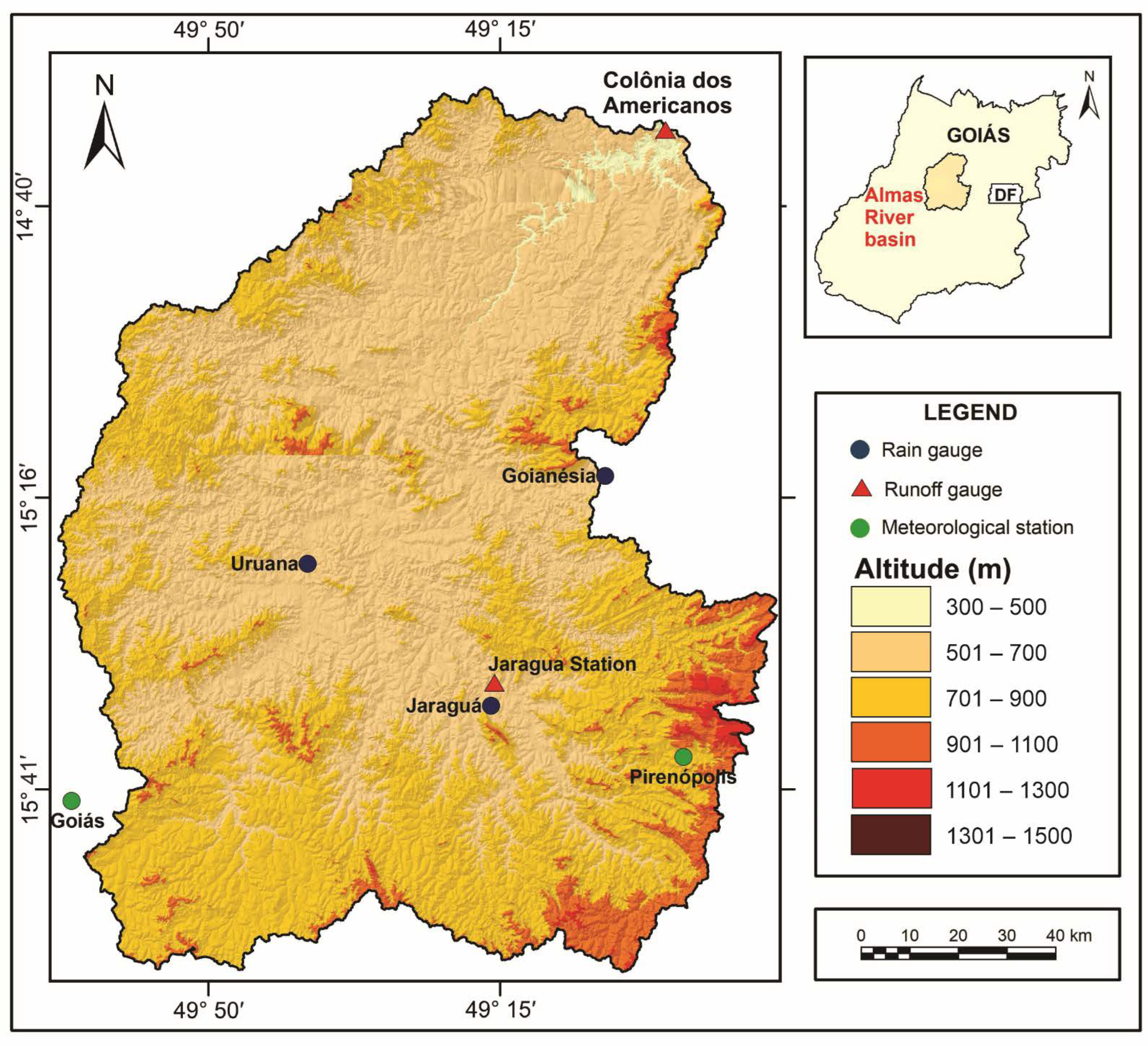
The Almas River basin has an area of 18,838 km² and is within the Cerrado biome. This basin is located between latitudes 14°37′00″ S and 16°15′00″ S and longitudes 50°08′00″ W and 48°49′00″ W (Figure 1). The Cerrado biome occupies an area of approximately 2,036,448 km² (24%) of the territory of Brazil. It is the second-largest biome in South America [5], recognized for the variability of the phytophysiognomy and the biodiversity of its flora and very rich fauna, with numerous species of plants and animals [38]. From a hydrological point of view, the Cerrado biome plays a fundamental role in producing water that flows into the main Brazilian river basins, such as Tocantins-Araguaia, Amazonia, Paraná, Paraguay, and São Francisco [39]. The Almas River basin is fundamental for energy generation, as is the Serra da Mesa Hydroelectric Power Plant, located in the basin outlet. This hydroelectric plant was inaugurated in March 1997 with a water volume capacity equivalent to 54.4 billion m³ [40]. This plant is essential for power generation, supporting South, Southeast, Midwest, and North Brazil [41]. This basin has species of heterogeneous vegetation with arboreal and forest, herbaceous-shrubby, and herbaceous-grassy strata, with spaced and gnarled trees, which are generally endowed with thick bark deep roots [42]. This basin is represented by several phytophysiognomies, such as savannah formations (Cerradão/Forest and typical Savanna), grassy formations (grassy field, clean field, and rupestrian field), and forest formations (riparian forest, gallery forest, dry forest, and Cerradão).

According to the Köppen classification, the region’s climate is Aw type (warm sub-humid tropical), and the average annual rainfall is approximately 1800 mm [43]. This region is marked by two well-defined seasons, a rainy season from October to April, with an average monthly rainfall of 250 mm, and a dry season from May to September with an average monthly of 10 mm [44]. The primary meteorological phenomenon that influences rainfall in the region during the rainy season is the South Atlantic Convergence Zone, formed from the arrival of subtropical fronts in central Brazil and is associated with moisture from the Amazon region, favoring the occurrence of rainfalls with large volumes [45]. Temperatures in the basin range from 17 °C to 34 °C, with an average relative humidity of approximately 80% [46].

The population in this basin is approximately 729,108 inhabitants, being mainly composed of an urban population (89%) [47]. The demographic structure of the basin has undergone an intense transformation since 1970, when the population changed from rural to urban. This phenomenon directly results from the change in economic and production base that this region has gone through. The expansion of the industrial park, notably that of agribusiness, and the strengthening of the service sector, boosted the local economy, attracting immigrants [48].

This basin has a great diversity of habitats. Since the 1970s, this region has suffered several environmental impacts on flora due to fragmentation and habitat loss, which affect the region’s fauna [49]. These modifications cause a disturbance and dispersion of the gene flow, influencing population density and genetic diversity, and occasionally causing local extinctions [50]. In addition to the local and regional effects of agricultural activities, global change is another critical factor that can impact the diversity and distribution of animal species such as the Quenquém (Acromyrmex diasi) and Ground-web Spider (Anapistula guyri) [49], and vegetation such as the Baru tree (Dipteryx alata Vogel) [50]. According to Ref. [49], there are currently more than 130 species of amphibians, birds, aquatic invertebrates, terrestrial invertebrates, mammals, fish, and reptiles in the Cerrado biome that are threatened with extinction.

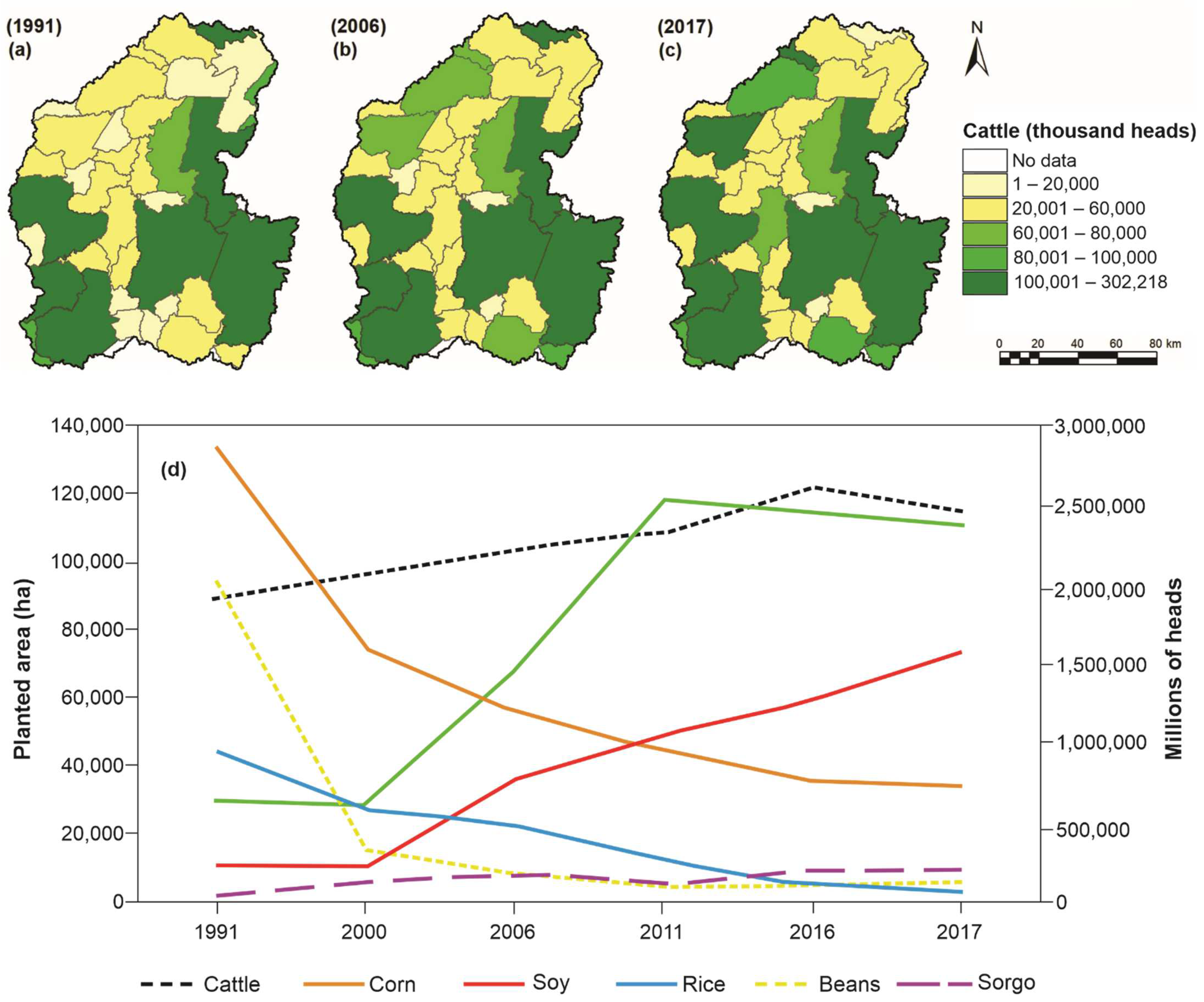
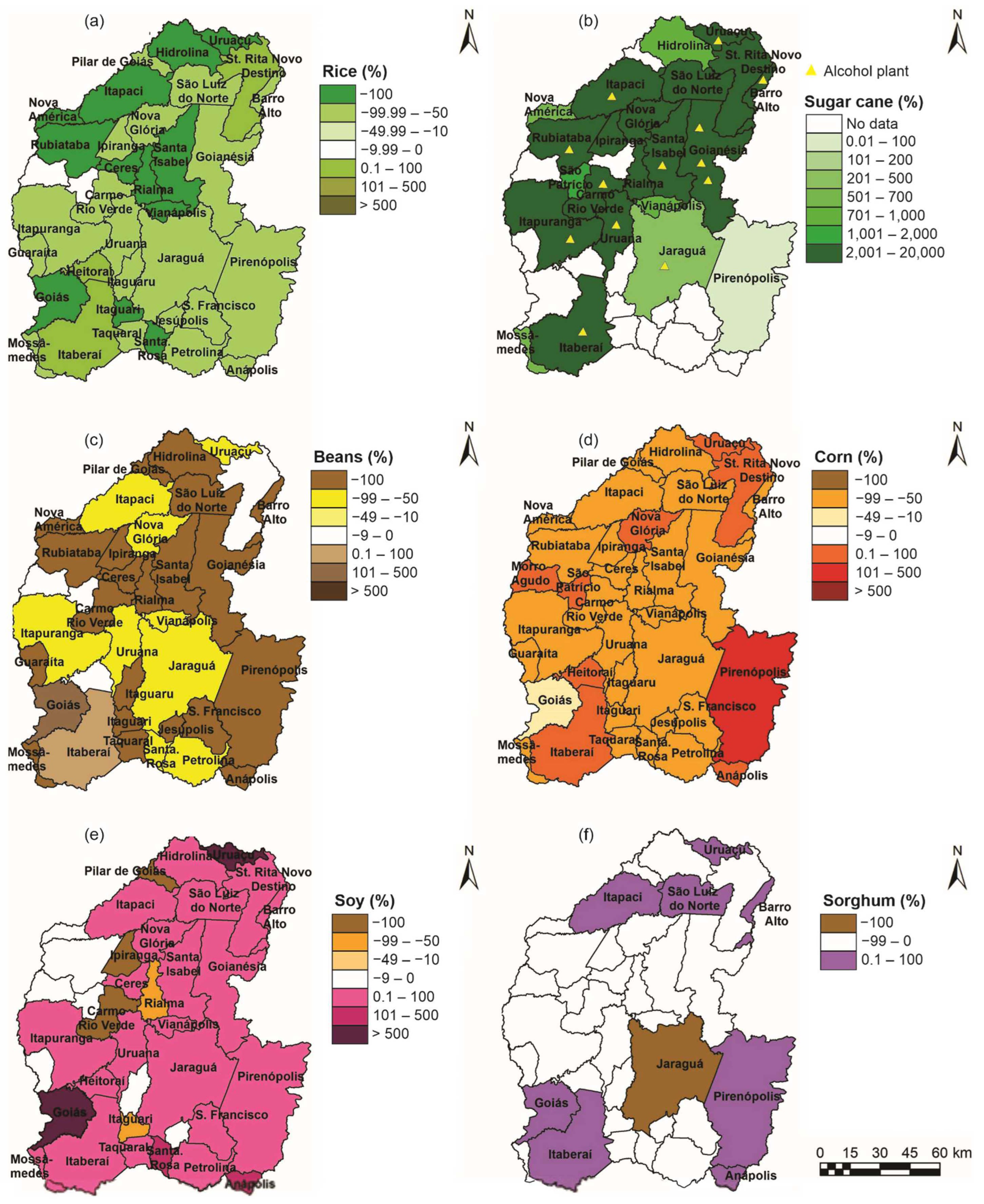
There are large extensions of crops with intense mechanization and significant investments in technology and inputs in the Almas River basin. The region’s crops are also characterized by the diversification of products, such as rice, sugarcane, beans, corn, soy, and sorghum. Agricultural production in the region is geared towards meeting regional particularities and commercial prospects as the demand for the products in international markets increases [51,52].

2.2. Evolution of Agriculture in the Region

This study collected data on the planted area of temporary agriculture of rice, sugarcane, beans, corn, soybean, and sorghum for 1991, 2000, 2006, 2011, and 2017 [53]. These years were chosen due to the advance of LULCC for agriculture and livestock. The data are available on the Automatic Recovery System (SIDRA)/Municipal Agricultural Production platform [54]. In addition, the data from the Municipal Cattle Raising Survey for 1991, 2000, 2006, 2011, 2016, and 2017 were also used to analyze the impact of changes in LULC arising from cattle ranching. These databases are the only official agricultural data sources in Brazil [53,54,55,56,57].

2.3. Hydrometeorological and Sediment Yield Data

Several data were used, such as the daily data of maximum and minimum air temperatures (°C), incident solar radiation (MJ/m²/day), wind speed (m/s), and relative air humidity (%) from the Pirenópolis and Goiás meteorological stations. These data are from 1971 to 1994 and were collected from the Meteorological Database for Teaching and Research platform [58]. Those data were used in the modeling to analyze the behavior of the hydrological processes within the basin. For the rainfall time series, daily data from five rain gauges from 1971 to 1994 were used: Jaraguá (ID #01549003), Uruana (ID #01549009), HPP Serra da Mesa Fazenda Cajupira (ID #01449005), Goianésia (ID #01549001), and HPP Serra da Mesa Ceres (ID #01549000) (Figure 1). In addition, streamflow data were acquired for the following stream stations: Colônia dos Americanos (ID #20490000) and Jaraguá (ID #20100000), for the period from 1974 to 1994. Rainfall and streamflow data were obtained from the website of the National Water Agency [59].

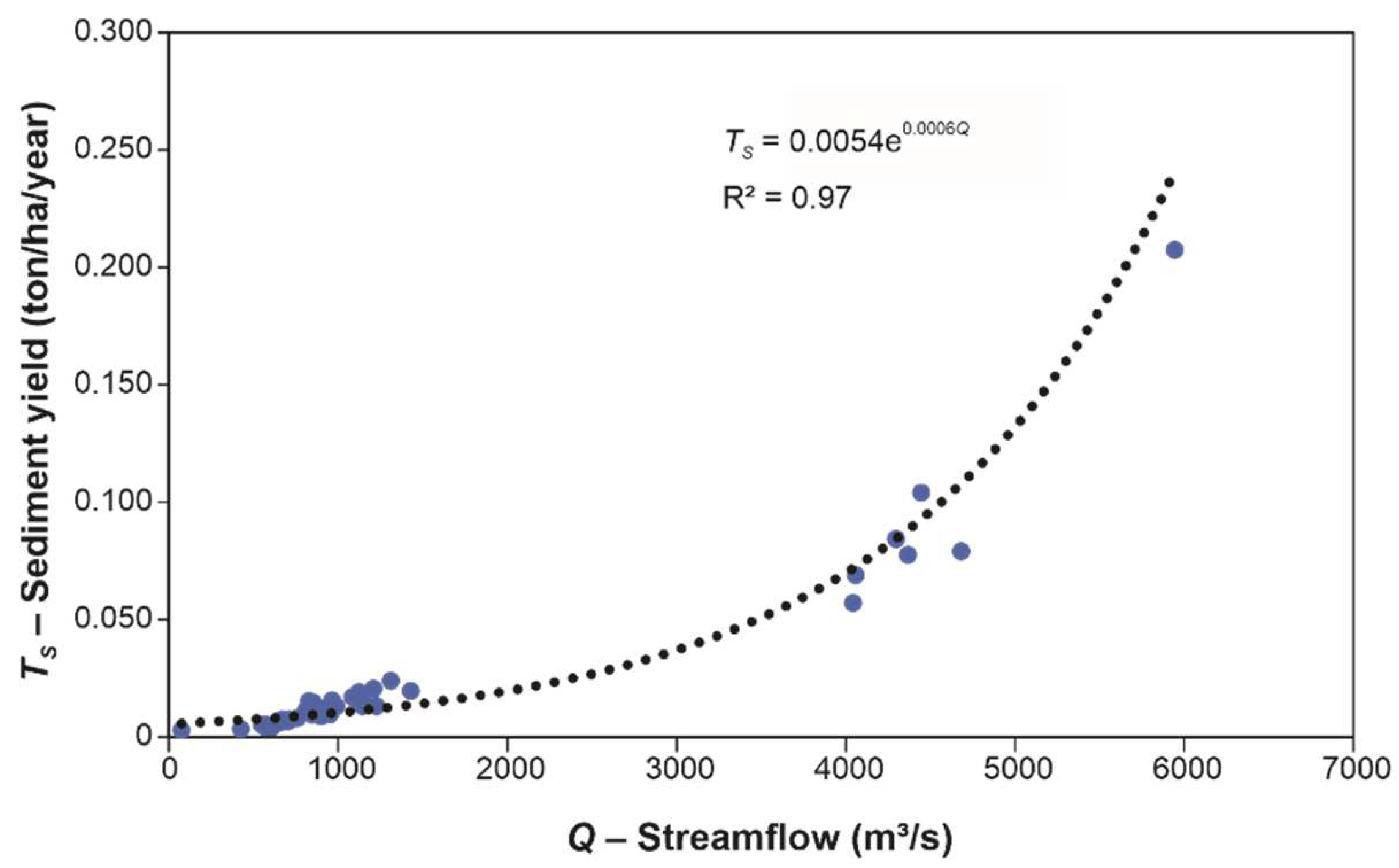
The validation of the SWAT model was performed by comparing calculated and observed sediment yield data. The estimated sediment yield (T_S), in ton/ha/year, was determined according to:

$$T_S=0.0864\times Q\times C_{SS}$$

(1)

where Q is the water discharge (m³/s), and C_SS is the suspended sediment concentration (mg/L). After calculating the suspended sediment discharge for each measurement, the sediment rating curve for each station was then established. Two criteria were used to evaluate the sediment rating curve quality: (a) the first was that the R² value must be higher than 60%, and (b) the second involved a visual assessment of how closely the exponential form of the generated curve followed the measured points.

The annual sediment transported by the Almas River basin was calculated, taking into account the discharge curve and the daily water flow dataset, the latter of which was obtained from the National Water Agency [59]. To develop this curve, total solids in the water and the respective discharge were collected between 2000 and 2019 in the São Félix do Araguaia gauging station (code 26350000), located near the study area, more precisely between coordinates latitude 11°37′02″ S and longitude 50°40′10″ W. Measured C_SS data were collected, which generated a good correlation curve between the flow data and the measured suspended sediment. After 2019, data were not used because the monitoring at the gauging station was discontinued after this date. The relationship between T_S and observed discharge was obtained, which presented an R² greater than 0.95 (Figure 2). In addition, the results obtained were discussed and compared to other studies, i.e., [60,61,62].

2.4. SWAT Model

In the SWAT, the land phase of the streamflow process, the driving force behind the movement of sediments, nutrients, or pesticides, was examined. In the SWAT model, the water balance is based on the following equation:

$${\mathrm{SW}}_t{=\mathrm{SW}}_0+{\displaystyle \sum _{i=1}^t\left(P_i-Q_i-E_{T_i}-R_i-Q_{G_i}\right)}$$

(2)

where SW_t is the final soil water content (mm), SW₀ is the initial soil water content on day i (mm), t is the time (days), P is the rainfall depth for the day i (mm), Q is the amount of daily streamflow on day i (mm), E_T is the amount of evapotranspiration on day i (mm), R is the amount of water entering the vadose zone from the soil profile on day i (mm), and Q_G is the amount of return flow on day i (mm).

The streamflow was estimated using the Soil Conservation Service (SCS) curve number (CN) method. The amount of daily streamflow is given as:

$$Q=\frac{{\left(R-I_a\right)}^2}{\left(R-I_a+S\right)}$$

(3)

where I_a is the initial abstractions, including surface storage, interception, and infiltration prior to runoff (mm), and S is the retention parameter (mm). The retention parameter is defined as:

$$S=25.4\times \left(\frac{1000}{CN}-10\right)$$

(4)

where CN is the applicable curve number for the day. The initial abstractions, I_a, is commonly approximated as 0.2 × S; hence, Equation (3) can be given as:

$$Q=\frac{{\left(R-0.2\times S\right)}^2}{\left(R-8\times S\right)}$$

(5)

The peak streamflow rate, which is the maximum runoff rate that occurs with a given rainfall event, is an indicator of the erosive power of a storm. It is used to calculate the sediment loss from the unit. SWAT calculates the peak runoff rate with a modified rational method, which is given as:

$$q_{peak}=\frac{C\times I\times A}{3.6}$$

(6)

where q_peak is the peak runoff rate (m³/s), C is the runoff coefficient, I is the rainfall intensity (mm/h), A is the sub-catchment area (km²), and 3.6 is a unit conversion factor from (mm/h) (km²) to m³/s.

The SWAT model uses the soil evaporation compensation factor (ESCO) to estimate the evaporation distribution better. The ESCO parameter must be between 0.01 and 1.0 and is used to adjust the depth distribution for evaporation from the soil to account for the effect of capillary action, crusting, and cracks. Calibrating this parameter is considered critical since it may vary from one catchment to another, even within the same geographical area. As the value for ESCO is reduced, the model can extract more of the evaporative demand from lower levels. ESCO coefficient is a calibration parameter and not a property that can be directly measured.

The SWAT model calculates sediment yield for each sub-basin using the Modified Universal Soil Loss Equation (MUSLE) [63]. MUSLE is a modified version of the Universal Soil Loss Equation (USLE) [64]. The MUSLE is given as:

S_Y = 11.8 × (Q × q_p × A_h)^0.56 × K × C × P × LS × CFRG

(7)

where S_Y is the sediment yield on a given day (t), Q is the surface runoff volume (mm), q_p is the peak runoff rate (m³/s), A_h is the area of the hydrologic response units (HRU) in ha, K is the soil erodibility factor (t·ha/MJ/mm), C is the USLE cover and management factor (dimensionless), P is the USLE support practice factor (dimensionless), LS is the USLE topographic factor, and CFRG is the coarse fragmentation factor (dimensionless).

The SWAT allows simultaneous computations in each sub-basin and routes the water, sediment, and nutrients from the sub-basin outlets to the basin outlet. The routing model consists of two components, deposition and degradation, which operate simultaneously. The amount of sediment finally reaching the basin outlet, S_out, is given as:

$$S_{out}=S_{in}-S_d+D_t$$

(8)

where S_in is the sediment entering the last or final reach, S_d is the sediment deposited, and D_t is the total degradation. The total degradation is the sum of re-entrainment and bed degradation components, and it is given as:

$$D_T=\left(D_r+D_B\right)\times \left(1-D_R\right)$$

(9)

where D_r is the sediment re-entrained, D_B is the bed material degradation component, and D_R is the sediment delivery ratio. Detailed theoretical documentation for the model is given by Neitsch [65]. More information about SWAT’s equations can be founded in Arnold et al. [66], Silva et al. [67], Gassman et al. [68], and Neitsch et al. [69].

2.5. Application of the SWAT Model and Performance Indices

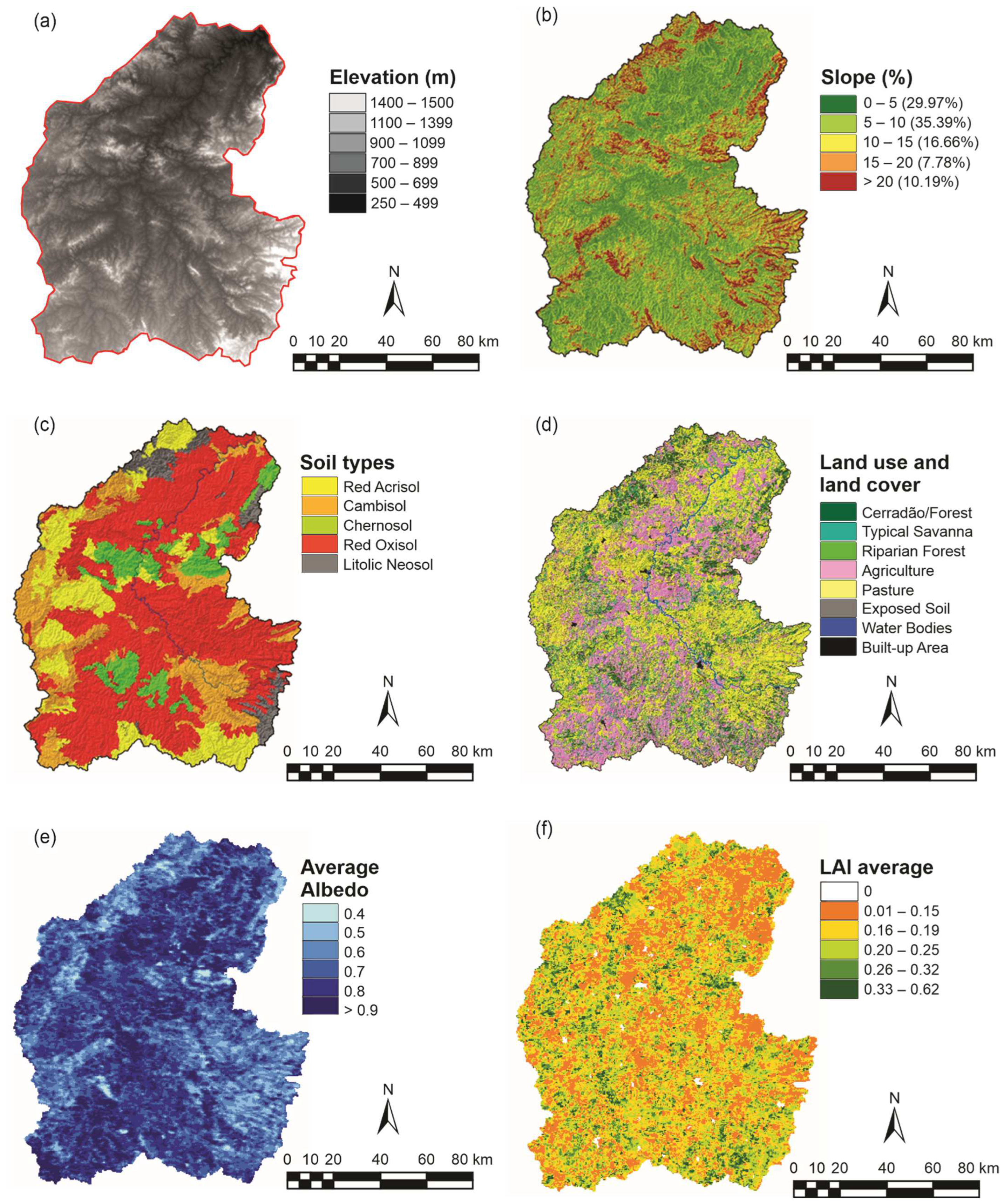
The Soil and Water Assessment Tool (SWAT) model [66] simulated the streamflow and sediment yield using different LULC scenarios for the Almas River basin. SWAT is a semi-distributed and continuous over time model that simulates the streamflow and sediment yield processes for long periods. The digital elevation model (DEM) used for the SWAT application was the Shuttle Radar Topographic Mission (SRTM) 1 Arc-Second Global, with a resolution of 30 m × 30 m. This DEM was used to determine the sub-basins (Figure 3a) and the slopes within the basin (Figure 3b). In this study, the LULC used in the modeling was obtained from Landsat 5/TM images (Figure 3c) path 222, and rows 070 and 071, downloaded from the USGS platform [70].

In this study, we chose to define the scenarios using Landsat image classification based on the research team’s expertise in the chosen method and its knowledge of the study area. The classification validation process was based on the confusion matrix, using the user’s accuracy, producer’s accuracy, omission, and commission measures [71]. Fieldwork in the basin was carried out during research development when data on LULC were collected to check the errors and successes of the classification. The classified map was statistically tested with random validation samples collected from orbital imagery and samples verified in the field. An independent collection of points of each LULC class was used to validate the classified classes that remained unchanged in the analyzed image. A group of 800 samples was randomly selected after image fusion and checked in the field.

The accuracy statistics for the classification and image commission, and the omission results, showed that the accuracy ranged from 81.5% to 84.6%, and the kappa coefficient ranged from 86.6% to 89.9%. The overall kappa coefficient and overall accuracy calculated for the entire image were 89.3% and 79.7%, respectively. The results of commission and omission show that all classes had suitable adjustments in the classification. To analyze the accuracy of image classification, the kappa index was used. This test is a discrete multivariate measure of actual concordance minus the concordance due to chance [1,3] (i.e., it is a measure of the consistency between the classification and the reference data). The kappa index (κ) can be calculated by:

$$\mathsf{\kappa }=\frac{D_o-D_e}{1-D_e}$$

(10)

where D_o represents the accuracy of the observed classifications, and D_e represents the accuracy of the expected classifications.

The soil map (Figure 3d) used was on a 1:250,000 scale [72]. The albedo data were obtained from the MCD43A3 V6 Albedo Model dataset (Figure 3d), a product used daily for 16 days, with spatial resolution of 500 m, for the 2000–2018 period [73]. The LAI was obtained using the MCD15A3H V6 level 4, a product from a 4-day composite dataset with spatial resolution of 500 m (Figure 3e). For this product, the algorithm chooses the best pixel available from all the acquisitions of both MODIS sensors located on NASA’s Terra and Aqua satellites within 4 days [74]. Albedo and LAI data were used for simulations using the SWAT model with grids at 500 m. All spatial bases were processed using ArcGIS 10.2^® software.

2.6. Calibration, Validation, and Sensitivity Analysis

The Nash–Sutcliffe (NS) efficiency coefficient [75], the Pearson coefficient of determination (R²), and the BIAS percentage (PBIAS) were used to evaluate the efficiency of the simulated data in the SWAT model. In addition, the performance of the calibration and validation results of the SWAT model was assessed based on the criteria recommended by Moriasi et al. [76]. These criteria establish guidelines for evaluating the model’s performance by comparing observed and simulated values. A perfect simulation, which is unlikely to happen, would have NS = 1, R² = 1, and PBIAS = 0%. The calibrated parameters and initial intervals are summarized in

Table 1. Parameters and ranges of variation used in the model calibration.

Parameter	Description	Inferior Limit		Upper Limit		Initial Simulation		Best Found Value		Adjusted Value		Method
		SWATd	SWATrs	SWATd	SWATrs	SWATd	SWATrs	SWATd	SWATrs	SWATd	SWATrs
ALPHA_BF	Baseflow alpha factor (days)	0	0	1	1	0.048	0.048	0.7871	0.7871	0.7871	0.7871	−
CN2	Initial SCS runoff curve number for moisture condition II	−1	−1	100	100	79	79	−0.407249	−0.407249	47	47	×
SOL_K	Saturated hydraulic conductivity (mm/h)	−0.8	−0.8	100	100	2.3	2.3	15.49457	15.49457	38	38	×
ESCO	Soil evaporation compensation factor	0.5	0.5	1.0	1.0	0.95	0.95	0.7195	0.7195	0.7195	0.7195	−
GW_DELAY	Aquifer recharge time (days)	−30	−30	450	450	31	31	168.5042	168.5042	199.5042	199.5042	+
SURLAG	Delay coefficient of runoff (dimensionless). Smaller values represent greater delay in runoff	0	0	24	24	2	2	20.7109	20.7109	20.7109	20.7109	−
SOL_AWC	Available water capacity of the soil layer (mm water /mm soil)	−0.25	−0.25	1	1	0.18	0.18	0.189402	0.189402	0.218	0.218	×
CH_N2	Manning’s n value for the main channel	0	0	0.3	0.3	0.014	0.014	0.176768	0.176768	0.176768	0.176768	−
GWQMN	Threshold depth of water in the shallow aquifer required for return flow to occur (mm water)	0	0	1000	1000	1000	1000	826.7252	826.7252	826.7252	826.7252	−
RCHRG_DP	Deep aquifer percolation fraction	0.1	0.1	1	1	0.05	0.05	0.767757	0.767757	0.088	0.088	×
GW_REVAP	Groundwater coefficient	0	0	0.2	0.2	0.02	0.02	0.1473	0.1473	0.1473	0.1473	−
CANMX	Maximum water storage in the vegetative canopy (mm)	0	0	100	100	0	0	52.6664	52.6664	52.6664	52.6664	−
SOL_ALB	The ratio of the amount of solar radiation reflected by a body to the amount incident upon its soil albedo	—	0.10	—	0.80	—	0.10	—	0.70	—	0.70	−
BLAI	Potential maximum of leaf area index for the plant	—	0	—	7	—	0	—	3	—	3	−

Values: substitution (−), addition (+), and multiplication (×).

.

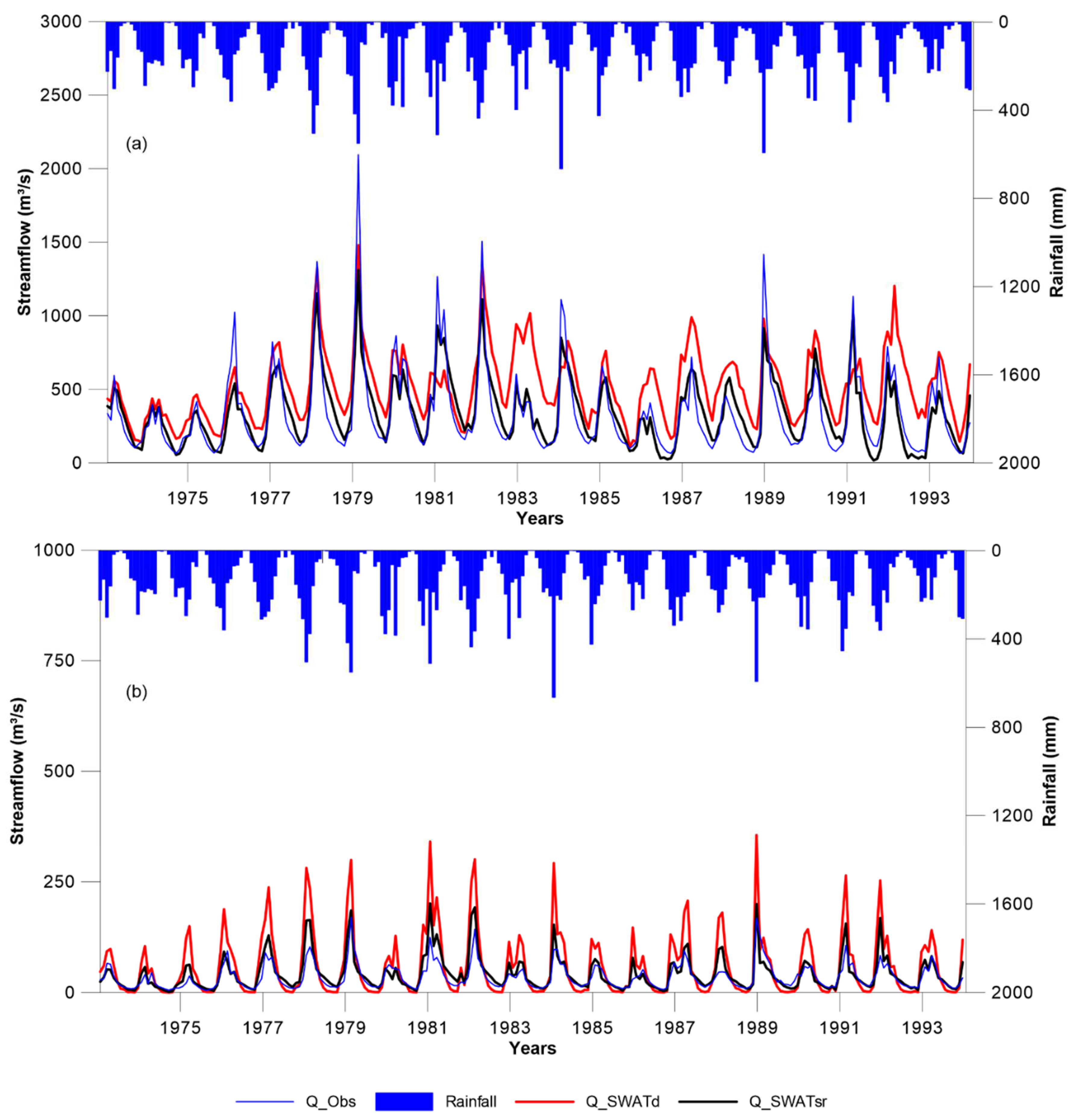
The calibration of the SWAT model was performed using the observed streamflow data from the Jaraguá and Colônia dos Americanos streamflow stations for the period from 1 January 1974 to 31 December 1980. The period for the validation process was from 1 January 1985 to 31 December 1994. The SWAT model possesses many parameters that can be used; thus, the most sensitive parameters were initially analyzed during the calibration process. This procedure was possible using the SWAT calibration and uncertainty program—SWAT-CUP [77]. To determine the parameter values in the calibration and the uncertainty of hydrological modeling, the Sequential Uncertainty Fitting (SUFI-2) algorithm [78] was used. Two sensitivity analysis methods were performed (i.e., the Latin hypercube and the one-factor-at-a-time methods [77]). A sensitivity analysis was performed using these two methods, based on observed and simulated streamflow data. 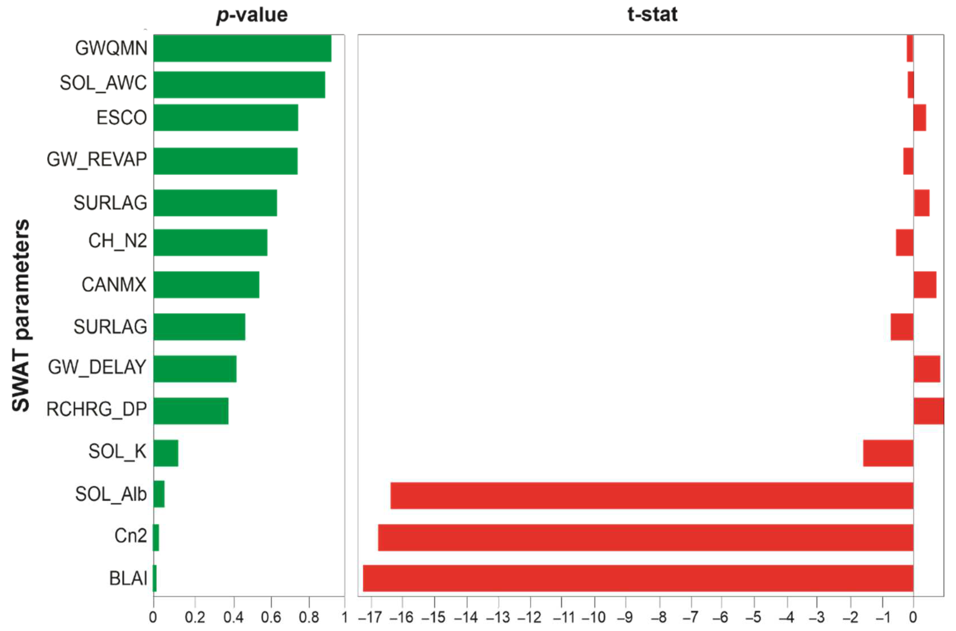The percentage of measured data bracketed by the 95% prediction boundary (p-factor) was used to quantify all the uncertainties associated with the SWAT model [79]. In this study, a sensitivity analysis of the SWAT model parameters was performed using t-stat and p-value [61]. The t-stat was used to provide a sensitivity measurement, and the higher its value is, the more sensitive the parameter would be. After this step, 19 parameters were selected for further calibration.

The SWAT model was applied based on two datasets: (1) without RS data and (2) using RS data obtained using GEE. The RS data corresponded to soil albedo and LAI. These parameters are highly complex and challenging to obtain in the field. RS-estimated values can improve the calibration of physically-based models, such as the SWAT model, for ungauged or poorly gauged basins; thus, this study involves essential RS products obtained by the MODIS sensor using advanced techniques in the GEE environment. Both products and techniques used in this study are of great interest to the geo-information user community, which focuses on hydrological modeling. Finally, the data were downloaded and organized into the standard SWAT input format.

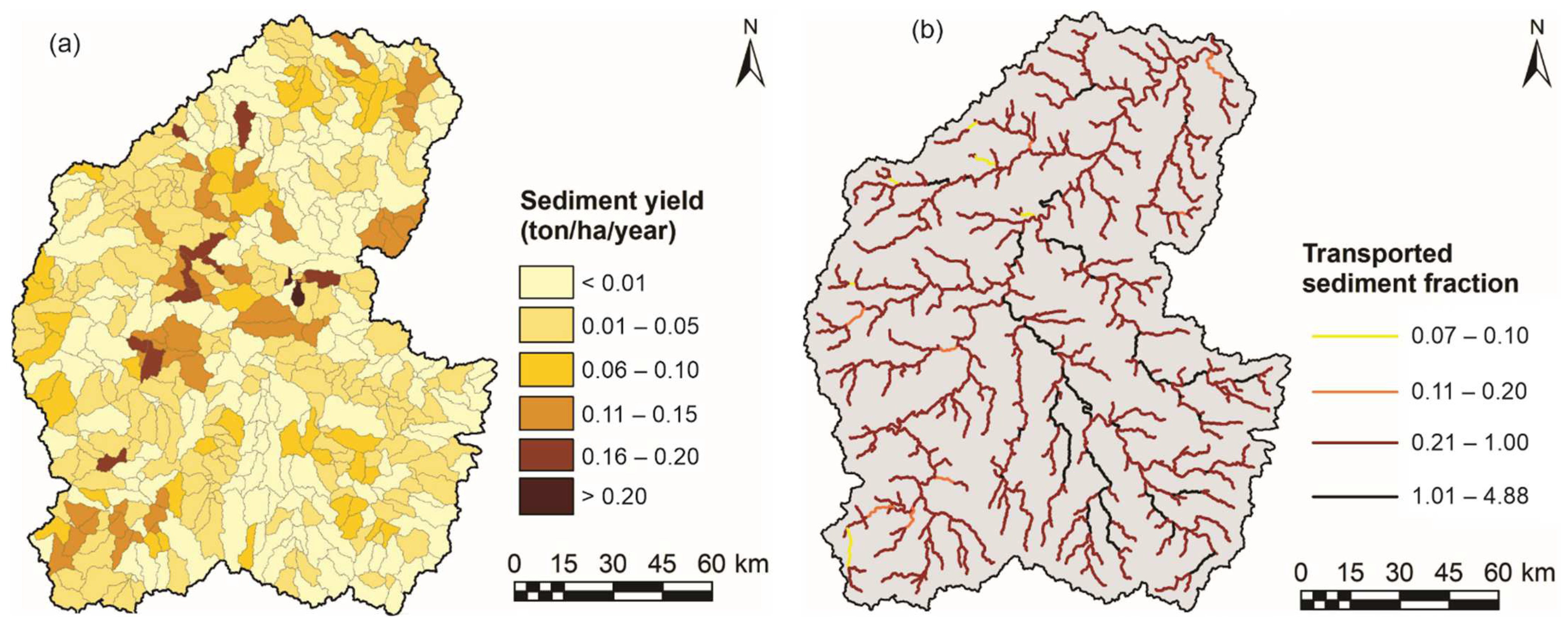
Landsat and SRTM data have the exact spatial resolution. They are imported directly into the SWAT model, which discretizes the basin into portions that possess unique land use/management/soil attributes, called HRU. The MODIS data, which have a spatial resolution different from the others, were treated and organized in a regular grid of 10 km. These datasets were imported into the SWAT model in tabular format, representing a regular mesh of stations. In this study, the sediment yield was divided into classes to represent better the spatialization of the results obtained. As described in

Table 2. Classes for sediment yield used in this study.

Number	Class	Sediment Yield (ton/ha/Year)
1	Very low	<0.01
2	Low	0.01–0.05
3	Moderate	0.06–0.10
4	High	0.11–0.15
5	Very high	0.16–0.20
6	Extremely high	>0.20

, the data were classified to represent the spatialization of the sediment yield in the study area.

2.7. Recent Changes in LULC and Future LULC Scenarios

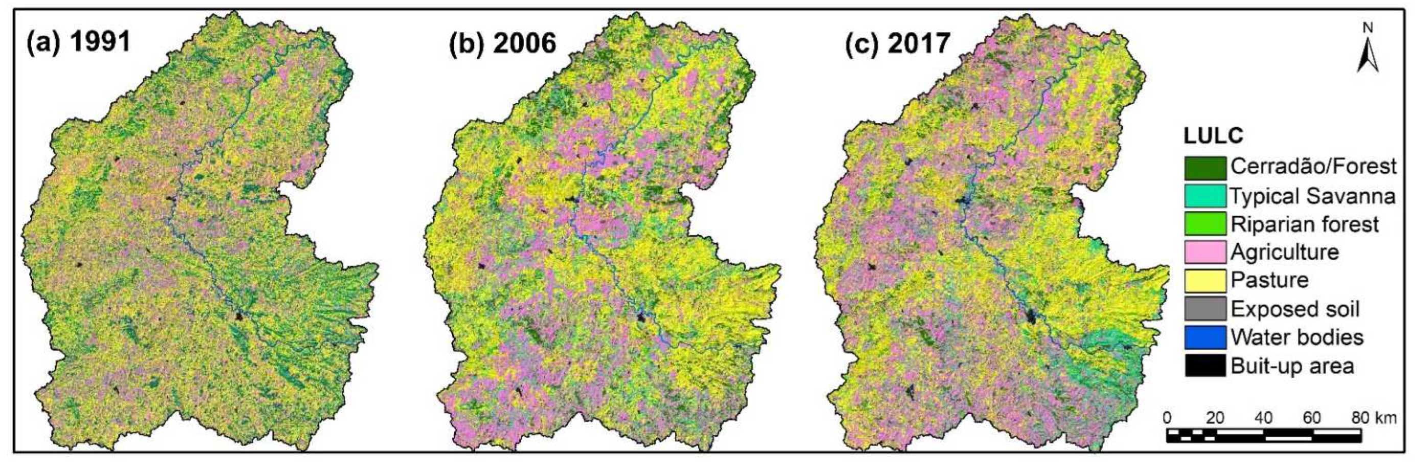
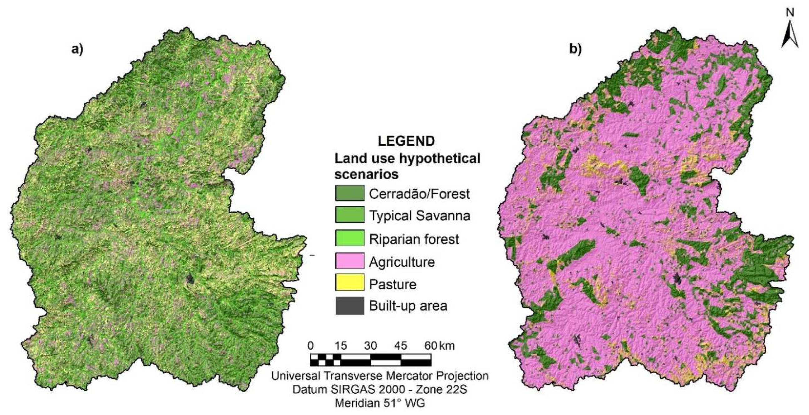
The years 1991, 2006, and 2017 were analyzed to assess changes in LULC. These years were selected because they contain dates with available images without clouds and with the most prolonged time interval to analyze changes in LULC for this basin. The LULC classification was performed using the maximum likelihood unsupervised classification method. The mappings used in this study were (a) LULC for 1991 (S1) using images from the TM/LANDSAT-5 sensor dated 13 June 1991, (b) LULC for 2006 (S2) using images of the TM/LANDSAT-5 sensor dated 13 June 2006, and (c) LULC for 2017 (S3) using images from the OLI/LANDSAT-8 sensor dated 13 June 2017. For the Almas River basin, the LULC identified were the following classes: cerradão/forest, typical Savanna, riparian forest, agriculture, pasture, and built-up area.

Two hypothetical LULC scenarios were proposed to evaluate the runoff–erosion processes in the basin, the (a) optimistic scenario (OS) and the (b) pessimistic scenario (PS). Based on the Brazilian forest code, the OS is considered the ideal LULC and was developed based on LULC S3 and the hypothetical recovery of permanent preservation areas close to watercourses, hilltops, and mountains. The future PS was simulated based on land use transformations that follow a historical trend in the basin, such as increased deforestation and growth in agricultural activities. The scenarios OS and PS were compared with observed and calibrated streamflows, the natural streamflow data measured at the streamflow stations, and simulated streamflow using the SWAT model based on the S1, OS, and PS scenarios. In addition, the OS maintained the existing native vegetation classes and estimated an increase in the remnant areas of the Cerrado biome (Cerradão/forest, typical Savanna, and riparian forest). The hypothetical PS is based on increased deforestation and the growth of agricultural activities, based on recent transformations of LULC that have taken place in recent years. The OS and PS scenarios were used as input data in the SWAT model, along with parameter values and meteorological data used in the calibration period. These simulations made it possible to compare the streamflow and sediment yield that occurred in these two scenarios with the simulations that took place in S1. Thus, the impacts of LULC changes on runoff–erosion processes are analyzed.

The different products used in this study aimed to provide the best historical representation of the analyzed processes. Unfortunately, the various datasets used do not have the same period. This limitation did not influence the methodology since the different products allowed for analyzing the phenomena separately. The integrated analysis of different products allowed a study in different stages: (a) LULCC, (b) simulation of LULC scenarios, (c) calibration and validation of the SWAT model with the longest existing time series, (d) validation of the sediment yield using the largest amount of data available, and (e) simulation of the runoff–erosion process in different LULC scenarios.

Table 3. Datasets, periods, and sources used in this study.

Dataset	Period	Source
Land use and land cover	1991–2017	https://earthexplorer.usgs.gov (accessed on 12 March 2021)
Agricultural production data	1991–2017	https://sidra.ibge.gov.br/ (accessed on 13 February 2021)
Weather data	1971–1994	http://www.inmet.gov.br/projetos/rede/pesquisa (accessed on 11 November 2021)
Hydrometeorological data	1971–1994	http://www.snirh.gov.br/hidroweb (accessed on 01 October 2021)
Albedo data	2000–2018	https://lpdaac.usgs.gov/products/mcd43a3v006 (accessed on 20 November 2021)
Leaf area index data	2000–2018	https://lpdaac.usgs.gov/products/mod15a2hv006 (accessed on 21 December 2021)
Total solid discharge	2000–2019	http://www.snirh.gov.br/hidroweb (accessed on 15 January 2022)

shows the period and source from which each product was obtained.

3. Results

3.1. Changes in LULC between 1991 and 2017

Figure 4a–c shows the spatial distribution of LULC in S1, S2, and S3. It is noticed that the agriculture and pasture classes occur in all portions of the basin and that in S3, there is an increase in these classes compared with S1 and S2. These classes predominate in the basin, and the agriculture class has constantly been increasing, whereas the pasture class showed a small oscillation. The results show that in S1, the agriculture and pasture classes accounted for 56.41% of the basin area. An advance can be seen in the agriculture and pasture classes, which influenced the growth of agriculture in the basin, mainly due to the increase in sugarcane being planted and cattle being raised in the area. Food crops of corn, beans, and rice were of lesser importance in the agricultural class of the region [20,21].

The results show that in S3, the agriculture and pasture classes occupy approximately 71% of the basin area. In comparison, the Cerradão/forest and typical Savanna classes occupy 21%, whereas the other classes occupy only 8% of the basin’s total area (

Table 4. Classified area and temporal variation of LULC for the Almas River basin.

LULC	S1 (1991)		S2 (2006)		Variation S1–S2 (%)	S3 (2017)		Variation S1–S3 (%)
	Area (km2)	Area (%)	Area (km2)	Area (%)		Area (km2)	Area (%)
Pasture	5427.32	28.8	6364.46	33.8	17.27	6791.82	36.1	25.14
Agriculture	3620.07	19.2	5790.45	30.7	59.95	6348.93	33.7	75.38
Cerradão/Forest	2366.42	12.6	2028.36	10.8	−14.29	2008.49	10.7	−15.13
Typical Savanna	1386.46	7.4	1936.24	10.3	39.65	1937.62	10.3	39.75
Riparian Forest	1566.73	8.3	1254.00	6.7	−19.96	956.39	5.1	−38.96
Exposed soil	1667.71	8.9	648.65	3.4	−61.11	402	2.1	−75.90
Water bodies	95.80	0.5	112.24	0.6	17.16	104.94	0.6	9.54
Urban area	40.61	0.2	55.78	0.3	37.36	86.64	0.5	113.35

). It should be noted that the pasture areas have expanded over the gently undulating and moderately undulating relief areas.

The results show that in S1, there was a decline in corn, bean, and rice areas, and a steady decline from S2 onwards. In the period analyzed, the planted area of sorghum remained practically unchanged due to it being used in conjunction with soybean and corn. The relationships concerning the runoff–erosion process are similar to those obtained in various studies [22,23], which analyzed the streamflow in river basins in the Cerrado biome. The results show that uncertainties were high because the basin has a significant heterogeneity of soil physical parameters; however, the statistical results obtained show a good fit between the observed and estimated data in the basin.

The transformations in the basin landscape between S1 and S3 occurred with the association of the crop–pasture system (i.e., a production system that prioritized some commodity crops, such as soybeans and sugarcane). In addition, it strengthened pasture areas that are cultivated with incorporated agriculture, which made the use of pasture in confinement more profitable. The increase in cropland reduced occupied areas with exposed soil, riparian forest, and cerradão/forest by −76%, −38.96%, and −15.13%, respectively (Table 4). The results show that the agriculture and pasture classes significantly increased (75.38% and 25.14%, respectively), while the typical savanna class increased by 39.75% (Table 4). The classes of native vegetation (Cerradão/forest, typical Savanna, and riparian forest) decreased by 7.8%. The change between S1 and S3 represented the scenario of the advance of agriculture in the region. The comparison between S1 and S3 is helpful to understand the total changes over the entire period studied.

3.2. Advances in Agriculture between 1991 and 2017

Figure 5a–c shows the number of cattle in S1, S2, and S3 for each municipality within the basin. The results show the municipalities that have the highest concentration of cattle within the basin, which are Pirenópolis, Goiás, Goianésia, Itapuranga, Itaberaí, Uruaçu, Jaraguá, and Barro Alto. Together, these municipalities have a total of 1,095,085 cattle (58.8% of the basin’s total). The results show that these municipalities grew by 18.6% during the study period, and that there was a more significant increase in the number of cattle in the municipalities in the southern portion of the basin (Figure 5c). It can also be highlighted that the municipalities of Santa Rosa de Goiás, Petrolina de Goiás, and Pilar de Goiás had a growth rate of 113.84%, 102.02%, and 101.66%, respectively. The cattle herd has expanded the number of cattle over the years, and the results show that the livestock area increased by 31% in the period. Figure 5d shows the areas planted with temporary crops and livestock between 1991 and 2017. As can be seen, the planted area data shows that soybean and sugarcane crops grew by 287% and 650%, respectively, whereas corn, bean, and rice crops showed a more significant decrease in the period analyzed. After 2000, the area planted with soybean crops predominated in the basin; therefore, such areas did not suffer reductions, even with the drop in the price of soybeans on the international market and the climate variations between 2006 and 2017. The same happened with the area planted with sugarcane because this crop had an appreciation in the international market during the same period. In addition, with tax incentives from the Government of Goiás State, new sugar and alcohol plants were reactivated and built, and improvements in the region’s agro-industrial complex enabled the expansion of sugarcane within the basin [37].

Figure 6a–f shows the spatial variation of the area planted with rice, sugarcane, beans, corn, soybean, and sorghum between 1991 and 2017 for each municipality within the basin. Figure 6a shows that most municipalities showed a decrease in the area planted with rice, and it is notable that the area planted with rice decreased by 96.9% between 1991 and 2017. The sugarcane planted area data show a significant increase in the period analyzed, and the incorporation of more municipalities in sugarcane production (28,972 ha in 1991 and 111,681 ha in 2017) represents an increase of approximately four times the area planted in the basin (Figure 6b). The results show that the area planted with beans within the basin showed a reduction of 95.4% (Figure 6c).

Figure 6d shows the spatiotemporal variation of the area planted with corn between 1991 and 2017. The results show a reduction of 75.4% in the period analyzed, which was similar to the cultivation of beans. On the other hand, the area planted with soybeans (Figure 6e) showed a significant increase (694.5%). Figure 6f shows the temporal variation from 1991 to 2017 in the area planted with sorghum. The results show an increase in the area with sorghum. The crop was spread in different portions of the basin (north and south), whereas the other areas did not show crop production, or they kept their planted area unchanged in the period analyzed.

3.3. Runoff–Erosion Modeling

3.3.1. Sensitivity Analysis

The results of the sensitivity of the best parameters assigned by SWAT-CUP are shown in Figure 7. The most sensitive parameters based on the p-value are grouped in descending order according to their greatest significance (i.e., closer to one). On the other hand, the t-stat is used to identify the relative significance of each parameter, estimating how changes in the value of a given parameter influence the results of the objective function. These two tests are used to analyze the sensitivity of the modeling (i.e., how the uncertainty in the modeling results can be attributed to different parameters that deal with the behavior of water in the basin, in such a way that it considers the entire amplitude of variation in the input data). Thus, the higher the p-value and the lower the t-stat value, the greater the sensitivity of the parameter in the modeling; therefore, it is not possible to group them by category. According to this figure, the most sensitive parameters in the modeling were CN2 and SOL_K. The other parameters that were also sensitive in the streamflow simulation were GWQMN, SOL_AWC, RCHRG_DP, GW-DELAY, SURLAG, CAMIX, CH_N2, ALFA_BF, GW_REVAP, and ESCO. The results show that the parameters which were considered more sensitive and influential for streamflow calibration are related to streamflow (CN2, SURLAG, and CH_N2), evapotranspiration (ESCO and CAMIX), soil water, and soil physical characteristics (SOL_K and SOL_AWC). It should also be noted that the groundwater parameters (ALFA_BF, GWQMN, GW_REVAP, GW_DELAY, and RCHRG_DP) were relevant in the modeling.

3.3.2. Calibration and Validation

Figure 8a,b shows the observed and simulated streamflow time series after model calibration for the Jaraguá and Colonia dos Americanos stations. The calibration results for the Jaraguá station showed a satisfactory fit between the observed and simulated monthly streamflow (R² = 0.8 and NS = 0.61) and in the validation period (R² = 0.76 and NS = 0.5). The annual average of the observed streamflow was 35.44 m³/s, whereas the simulated streamflow was 41.48 m³/s, a difference of 17%. The PBIAS value for the Jaraguá station in the calibration period was −20.3% and −28.5% in the validation, indicating an overestimation bias.

For the Colonia dos Americanos station, the results presented a very good performance in the calibration and validation, presenting R² = 0.85, NS = 0.82, and PBIAS = 0.9% for the calibration, whereas in the validation period, the values were R² = 0.84, NS = 0.80, and PBIAS = −15.5%. The Colonia dos Americanos station results also showed an overestimation bias to the observed values. The average observed streamflow was 337.80 m³/s, and the simulated streamflow was 360.60 m³/s, an increase of 6.74%, which can be considered low between the measured and simulated streamflow.

3.4. Estimate Sediment Yield

Figure 9a shows the spatial distribution of sediment yield in the Almas River basin between 1974 and 1994. Figure 9a also shows that the sediment yield is very variable and that the most significant amount of sediment occurs in the elevated regions, which are moderately wavy. The results show that the sediment yield in the sub-basins varied between 0.01 and 0.2 ton/ha/year. It is notable that the most significant volume of sediment occurred in areas with agriculture, pasture, exposed soil, and types of cambisols and red clay soils located in the eastern portion of the basin. In contrast, the smallest volumes of sediment occurred in areas with natural vegetation cover. The basin areas with agriculture, pasture, exposed soil, and red oxisol type soils, with slopes varying between 0% and 5%, had sediment yields between 0.01 and 0.12 ton/ha/year.

Figure 9b shows the sediment fraction that each segment of the drainage network transports to the subsequent channel stretch. Again, the pattern of the sediment fraction of river stretches can be seen located in the upper and middle portions of the basin, which show more significant sediment deposition. In contrast, the sub-basins close to the basin boundary had little or no sediment deposition.

Table 5. Observed and calculated sediment yield and estimation errors for the study area.

Years	Sediment Yield (ton/ha/Year)
	Observed	Calculated	Estimation Error (%)
Average	0.032	0.025	−21.88
Standard deviation	0.041	0.016
Mean deviation	0.031	0.013
Coefficient of variation	1.288	0.646

shows statistics of sediment yield and estimation errors between observed and calculated data. The results highlight that the calculated sediment yield underestimated the observed data by 22.42%. The curve fitting for the relationship between sediment yield and observed discharge presented R² equal to 0.97. This relationship can be considered very good due to the uncertainties in estimating sediments in rivers with a large volume of suspended sediments and non-continuous data collection. Furthermore, as the station used to measure the observed data is downstream of the Almas River basin (i.e., it has a water catchment area more extensive than the studied basin), it was expected that the data collected in situ would present an overestimation. This sediment measurement station is close to the basin outlet and past the Serra da Mesa hydroelectric plant; thus, the contribution area chosen as the study area comprises the catchment area up to the hydroelectric plant and the results of the SWAT model can be considered satisfactory.

3.5. Hypothetical Land Use Scenarios and Simulation of Runoff–Erosion Processes

Table 6. Land use class data for the two hypothetical land-use scenarios, simulated with the SWAT model.

LULC	Optimistic LULC (OS)		Pessimistic LULC (PS)
	Area (km2)	Area (%)	Area (km2)	Area (%)
Typical Savanna	4615.64	24.77	4312.03	23.14
Cerradão/Forest	4333.38	23.25	−	−
Pasture	3765.72	20.21	1181.39	6.34
Agriculture	3190.74	17.12	13,058.11	70.07
Riparian forest	2668.76	14.33	−	−
Urban area	62.59	0.34	85.31	0.46

and Figure 10a,b show the classes of hypothetical scenarios of optimistic and pessimistic LULC. The OS simulation results showed that the natural vegetation classes represent 63% of the basin’s total area (i.e., 23.25% Cerradão/forest, 24.77% typical Savanna, and 14.32% riparian forests). The agriculture, pasture, and urban area classes represent 17.12%, 20.21%, and 0.34% of the basin’s total area, respectively. The spatial distribution of the simulated LULC for the PS is shown in Figure 10b. The PS shows an intense change in land use, in which the natural vegetation was entirely replaced by agriculture (70.07%), pasture (6.34%), and urban area (0.46%), which represents 76.86% of the total area of the basin. The other LULC occupied 23.14% of the basin area (i.e., a reduction rate of 62.88% for the OS scenario). Changes in the PS indicate less protection against the direct impact of rainwater drops in the soil, which favors the runoff and the detachment and transport of sediment particles.

To assess the efficiency of the SWAT model, we compared simulated monthly average streamflow data based on hypothetical scenarios with the observed data. Figure 11 shows the SWAT model simulations for the OS and PS scenarios for the Colonia dos Americanos stations.

Table 7. Statistical comparison of mean streamflow and sediment yield for S1, OS, and PS scenarios.

Statistics	Rainfall (mm)	Streamflow (m3/s)			Sediment Yield (ton/ha/Year)
		S1	OS	PS	S1	OS	PS
Mean	1612.23	514.17	504.17	547.23	0.026	0.023	0.035
Maximum	2245.62	766.42	622.64	839.94	0.049	0.039	0.063
Minimum	1075.84	323.84	297.96	359.21	0.010	0.011	0.020
Standard deviation	285.70	133.66	104.56	140.74	0.011	0.007	0.011

presents the comparison of the observed, calibrated, and simulated streamflows for the OS and PS scenarios. The results of the monthly average streamflow for the OS showed that the simulated streamflow was 337.80 m³/s and the observed value was 455.88 m³/s, a difference of −25.9% for the Jaraguá station. For the Colonia dos Americanos station, the simulated streamflow was 504.17 m³/s and the observed value was 514.17 m³/s, a difference of −1.9%. The comparison between the observed and simulated streamflow using the PS at the Jaraguá station show that the streamflow was 500.44 m³/s, presenting an increase of approximately 9.8%. For the Colonia dos Americanos station, the simulated streamflow was 547.23 m³/s (i.e., a difference of 6.4%). The obtained coefficients of determination confirmed that the simulated flows accurately replicated the measured flows in the present research. The statistical indicators of the calibration and validation phases show the satisfactory performance of the model throughout the basin, mainly upstream and downstream. The obtained results follow other studies, which emphasize the good performance of the SWAT model in modeling Cerrado basins (e.g., [21,27,28,30,31,71]); therefore, the impacts of LULCC on the streamflow time series can be assessed using the calibrated and validated SWAT model.

Figure 12 compares annual differences in sediment yield for scenarios S1, OS, and PS. As can be seen, there is a significant discrepancy between the results of the three simulations. The results show an intensification of soil erosion when comparing the PS and OS, by approximately 54%. The results also show that the sediment yield in the OS scenario decreased by around 11% compared to the S1 scenario. LULC variation in the OS seems to cause less erosion and much more deposition than the S1 and PS variation. Comparing the S1 scenario with the OS, it is expected that native vegetation can reduce erosion, as it directly changes the infiltration parameters and especially the protection given to the soil against the direct impact of raindrops and increased surface roughness, as reported by [60].

Figure 13 shows the spatial distribution of sub-basin sediment yield classification in hypothetical optimistic (Figure 13a) and pessimistic (Figure 13b) land use scenarios. The results show that both LULC scenarios significantly influence the sediment yield since there are mainly occurrences of very low and low classes in the OS compared to PS. The total impact of the PS on the increase in the sediment yield is much more significant than in other scenarios; however, the differences comparing the OS and PS are not linear, mainly due to the different geographic locations occupied by native vegetation in both scenarios. As in OS, the LULC that predominated in steep areas was native forest vegetation, which acted as a barrier to sediments and areas with very low sediment yields. When the runoff passes from a sugarcane area to a native vegetation area, the flow velocity decreases because of the high surface roughness due to the vegetation. This characteristic of LULC reduces the sediment transport capacity, preventing them from reaching the drainage network due to the early sediment deposition. Considering that the riparian forest in the Almas River basin is in a good state of preservation, we can highlight how this LULC acts as a protective barrier to sediments, mainly reducing the flow rate and retaining sediments.

The results show that in the OS, there was a predominance of sub-basins classified as very low risk to erosion (88% of the basin), which can be due to the hypothetical regeneration of vegetation cover and linear corridors of riparian forest, which acted as a physical barrier to retain sediment from the slopes. The agricultural class occupied the sub-basins with greater erosion susceptibility with cambisol soils and slopes ranging from 0 to 5%. The erosion results in the PS were very variable, and the moderate erosion risk class was the one with the most significant predominance (71%). The results for the PS scenario showed that 50 sub-basins (10.3% of the basin area) presented sediment yield in the moderate class (i.e., such sub-basins are areas susceptible to the erosion process). When comparing the areas susceptible to sediment yield among the hypothetical scenarios, the OS had a significant increase of 1725.21% compared to the OS. The hypothetical simulated land use scenarios had significant differences. The optimistic scenario presented a very low to low risk of sheet erosion. In contrast, the other pessimistic scenario was unfavorable, presenting a high risk of erosion susceptibility and a high predisposition for the sediments to be transported to the drainage channels. These results highlight the importance of land cover in protecting the soil against erosion processes.

4. Discussion

Knowing the influence that changes in the LULC can have on the quantity and quality of sediments, and how streamflow can affect energy generation, ecosystems in the basin, and impact freshwater availability for human consumption and agro-industrial production, changes in the LULC influence streamflow and sediment yield behavior, as demonstrated in the simulations of the two LULC scenarios. The study highlighted that the increase in agricultural and pasture areas and the decrease in native vegetation cover caused severe environmental impacts, reinforcing the need to manage the LULC at a basin-scale in a biome such as the Cerrado. This methodology can be tested in ungauged or data-poor watersheds as it uses freely available datasets and consolidated and widely used methods. In addition, the applicability of this study allows the simulation of LULC future scenarios at a low cost, and it gives an estimation of streamflow and sediment yield time series.

The results of this study can help decision makers understand the changes to the landscape in recent decades and allow them to make future predictions about public policies for environmental preservation or the liberation of areas from pasture or agricultural activities. As a result, the OS and PS scenarios were proposed, and the streamflow and sediment yield behavior results were analyzed.

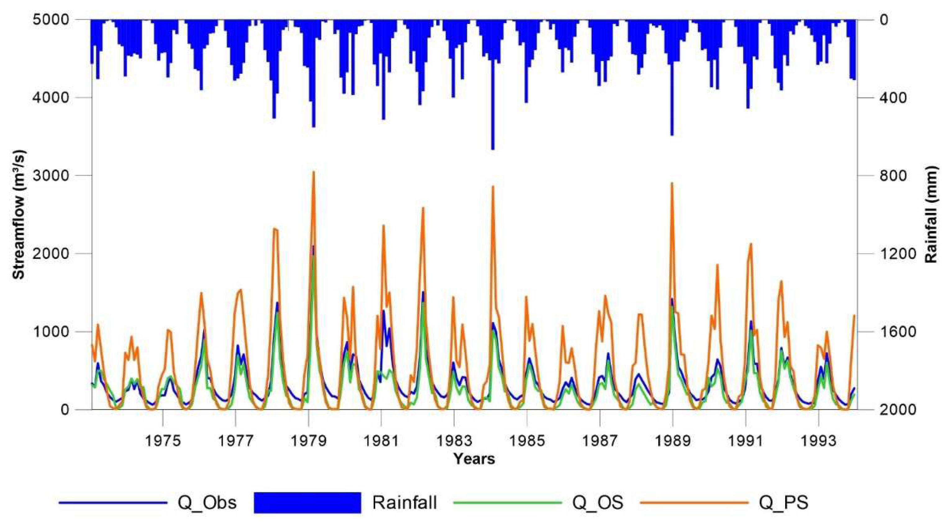
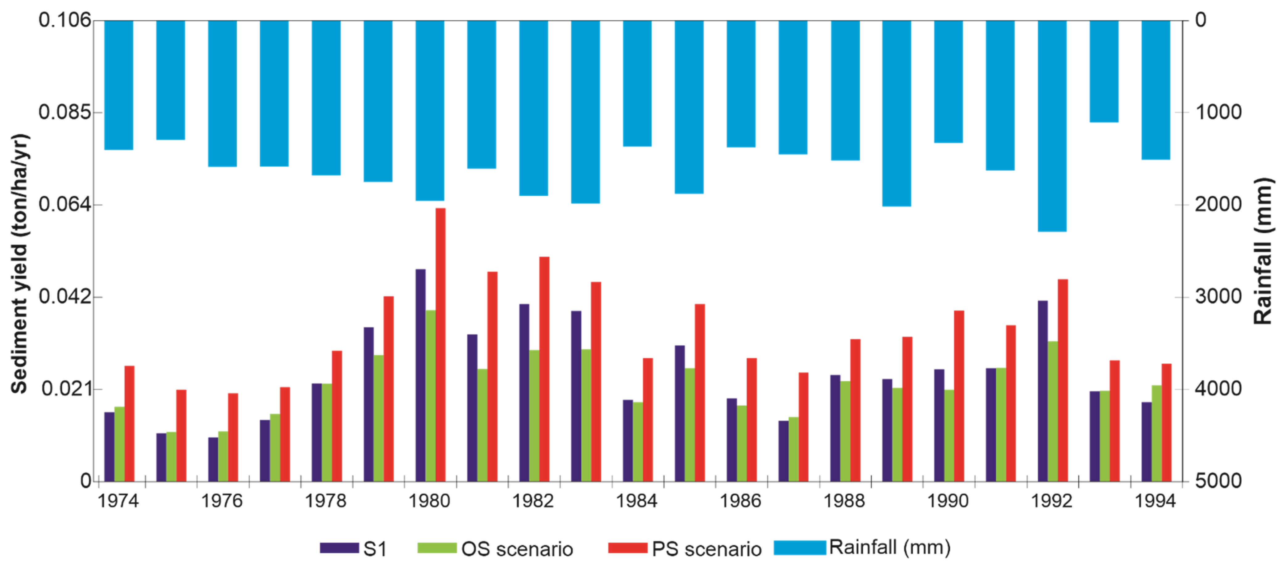
The calibration and validation results show that the LULCC in this region severely influence the streamflow pattern. The results of this modeling are similar to the results obtained in the Cerrado area by [29,30,32,33]. As expected, the sediment yield and streamflow results show that the highest values occurred in the PS, whereas a significant decrease was observed in the OS, considering the S1 scenario. The average annual sediment yield for the OS was 0.023 ton/ha/year, whereas for the PS, it was 0.035 ton/ha/year, representing a difference of 21.88% (Table 5). These results show that LULC greatly influences runoff–erosion processes in the region [67]. Vegetation cover plays a fundamental role in water conservation and supply, nutrient cycling, soil protection against erosion, temperature regulation, water cycling, and returning water to the atmosphere by evapotranspiration. For this reason, one may say that deforestation and LULCC are two of the world’s leading environmental concerns, especially in Brazil, which is currently the country that devastates its native vegetation most (e.g., the Cerrado biome).

The estimate of sediment yield in S1 shows a reduction of 10.96% in the OS, and when compared to the PS, it shows an increase of 37.4% (Table 5). These results highlight the influence of LULC as one of the main controlling factors of hydrological processes, as it was possible to compare the results of streamflow and sediment yield with the same amount of rainfall but with different conditions of LULC.

Changes in areas of the pasture class by native vegetation reduced the erosion process. According to Falcão [12], grazing under adequate conditions usually does not increase sediment in water bodies after heavy rains. Nevertheless, intensive grazing on sloping terrain and fragile soils can cause severe erosion problems. In addition, according to the authors, the sediment yield increases when riparian areas are used as pasture, which leads to erosion of the riverbanks and deposition directly on the bed. There is still no accurate data on erosion from cultivated areas in Brazil. According to USDA [80], for instance, in the United States, erosion generated in cultivated areas is approximately 38%, while pasture erosion accounts for 26% of the sediments reaching water bodies. According to Santos et al. [61] surface roughness is the main factor in reducing surface streamflow, and consequently, the sediment yield.

The hypothetical land use scenarios of the Almas River basin alerted possible future situations in a river basin for issues related to runoff–erosion processes. Taking rigorous measures to preserve the vegetation cover and reforestation implies reducing environmental impacts and sediment yield within the basin. In this context, the methodology adopted to generate these hypothetical scenarios allowed us to satisfactorily show that the hydrological processes associated with land use and management play a fundamental role in understanding the water and sediment yield within the river basin.

Despite the SWAT model’s many qualities, its limitations must be further discussed and analyzed. The SWAT model was developed for rural watersheds, and therefore, there is a need for parameter calibration; thus, identifying the parameters that have or do not have a significant influence on the model simulation is fundamental not only to reducing the modeling uncertainty but also to reduce the number of excessive parameters in the model calibration process, which can harm the physical representation of the basin in the model. In this regard, please see [61,67], which provide more details on SWAT’s capabilities and limitations.

5. Conclusions

This study evaluated the impacts of historical LULCC on hydrological processes using the SWAT model and remote sensing multiple gridded datasets for a humid tropical basin in the Cerrado biome in Brazil. With the calibration of the SWAT model, it was possible to observe that some parameters are more influenced by the runoff–erosion process than others, providing the conditions to improve the simulation in the basin. After validation, the hydrological simulation satisfactorily represented the streamflow variability and the estimated sediment yield during the period studied. The temporal evolution of the changes in the LULC increased the mean streamflow and the sediment yield. This study highlighted that the LULCC in the study area play an essential role in the runoff–erosion process in the Cerrado biome, and consequently, impacts various human activities such as agribusiness, livestock, energy production, food security, and public water supply. The purpose of the study was to simulate the influence of LULCC on the amount of streamflow and sediment yield in the basin in different scenarios. Nevertheless, the water quality in the basin was not analyzed due to the methodology tested. The results alert decision makers about the importance of proper LULC management in the streamflow and sediment yield in the basin.

This study discussed the LULCC due to agricultural advances that caused a shift in the runoff–erosion dynamics, exploring the applicability of remote sensing in an ungauged basin in the Cerrado biome in Brazil that underwent intense modification in LULC. The analysis of the LULCC for 1991, 2006, and 2017, and the agricultural census data, allowed us to understand the reconfiguration of the basin’s landscape over the twenty-six years, which proved to be fast and progressive in the process of expansion of the economic activity. This complexity involves replacing food grains (rice and beans) to incorporate crops in an area planted with sugarcane and soy and the expansion of cattle ranching. Reconciling the pressure of agribusiness with the preservation of natural areas is a challenge for environmental planning and management of water resources. The changes in LULC and deforestation interfere with the hydrological cycle, causing a reduction in water infiltration into the soil and increasing the streamflow, which affects the fluvial dynamics and erosion process. In addition, this paper demonstrated how LULC, soil parameters, albedo, and LAI obtained from RS datasets could successfully calibrate distributed hydrological models such as the SWAT model. This research showed that the influence of LULC on the runoff–erosion process using estimated satellite data and runoff–erosion models in the Cerrado biome is still scarce in Brazil. We can conclude that the current simulations are classified as good according to Moriasi [76].

The runoff–erosion modeling allowed us to understand the runoff–erosion process, helping the future planning and territorial management of water resources in this basin. This modeling also helps define public policies to control deforestation and preserve, maintain, and recover the Cerrado biome. From these future perspectives of land use in the hypothetical scenarios in different landscapes, it allowed us to analyze the responses in terms of the effects of anthropic action on the runoff–erosion processes within the basin.

The continuous agricultural activity in the basin permeates the confrontation and pressure from agribusiness on land regulation, the control of burning in the area in the Cerrado biome, and the lack of inspection and regulation of the forest code. Given the data from the pessimistic scenario simulated in the model, the trend is clear for the growth of social and environmental practices such as deforestation, climate change, water use for agricultural irrigation, water erosion, siltation of watercourses, and sediment yield, among others. It can be concluded that the parameters calibrated in this study are valid and correspond with all types of landscape and land use based on the performance of the SWAT model, and after comparing observed and calculated streamflow and sediment yield data. It can be concluded that estimated values of soil parameters obtained by remote sensing slightly improved the model’s calibration. These results can be significantly valuable to governmental agencies as a communication model for better water resource management and energy generation. Furthermore, these results are highly relevant to the sustainable management of water resources within the region, as such obtained results allow decision makers to observe how water variables behave with changes in LULC caused by human actions; thus, managers can know in advance in which sub-basins this conditioning is more prominent, especially in areas with remnants of forests, or areas characterized by the advance of agriculture in recent years.

References

1. Da Cunha, E.R.; Santos, C.A.G.; Silva, R.M.; Panachuki, E.; De Oliveira, P.T.S.; Oliveira, N.S.; Falcão, K.S. Assessment of current and future land use/cover changes in soil erosion in the Rio da Prata basin (Brazil). Sci. Total Environ. 2022, 807, 151811. [Google Scholar] [CrossRef]
2. Tirupathi, C.; Shashidhar, T. Investigating the impact of climate and land-use land cover changes on hydrological predictions over the Krishna river basin under present and future scenarios. Sci. Total Environ. 2020, 721, 137736. [Google Scholar]
3. Cunha, E.R.; Santos, C.A.G.; Silva, R.M.; Bacani, V.M.; Pott, A. Future scenarios based on a CA-Markov land use and land cover simulation model for a tropical humid basin in the Cerrado/Atlantic forest ecotone of Brazil. Land Use Policy 2021, 100, 105141. [Google Scholar] [CrossRef]
4. Verstegen, J.A.; van der Laan, C.; Dekker, S.C.; Faaij, A.P.C.; Santos, M.J. Recent and projected impacts of land use and land cover changes on carbon stocks and biodiversity in East Kalimantan, Indonesia. Ecolog. Indicat. 2019, 103, 563–575. [Google Scholar] [CrossRef]
5. Dos Santos, G.L.; Pereira, M.G.; Delgado, R.C.; Magistrali, I.C.; da Silva, C.G.; de Oliveira, C.M.M.; Laranjeira, J.P.B.; da Silva, T.P. Degradation of the Brazilian Cerrado: Interactions with human disturbance and environmental variables. Forest Ecol. Manag. 2021, 482, 118875. [Google Scholar] [CrossRef]
6. Korkanç, S.Y. Effects of the land use/cover on the surface runoff and soil loss in the Niğde-Akkaya Dam Watershed, Turkey. Catena 2018, 163, 233–243. [Google Scholar] [CrossRef]
7. Grecchi, R.C.; Gwyn, Q.H.J.; Bénié, G.B.; Formaggio, A.R.; Fahl, F.C. Land use and land cover changes in the Brazilian Cerrado: A multidisciplinary approach to assess the impacts of agricultural expansion. Appl. Geogr. 2014, 55, 300–312. [Google Scholar] [CrossRef]
8. Beuchle, R.; Grecchi, R.C.; Shimabukuro, Y.E.; Seliger, R.; Eva, H.D.; Sano, E.; Achard, F. Land cover changes in the Brazilian Cerrado and Caatinga biomes from 1990 to 2010 based on a systematic remote sensing sampling approach. Appl. Geogr. 2015, 58, 116–127. [Google Scholar] [CrossRef]
9. Ferreira, F.L.V.; Rodrigues, L.N.; da Silva, D.D. Influence of changes in land use and land cover and rainfall on the streamflow regime of a watershed located in the transitioning region of the Brazilian Biomes Atlantic Forest and Cerrado. Environ. Monit. Assess. 2021, 193, 16. [Google Scholar] [CrossRef] [PubMed]
10. Cunha, E.R.; Santos, C.A.G.; Silva, R.M.; Bacani, V.M.; Teodoro, P.E.; Panachuki, E.; Oliveira, N.S. Mapping LULC types in the Cerrado-Atlantic Forest ecotone region using a Landsat time series and object-based image approach: A case study of the Prata River Basin, Mato Grosso do Sul, Brazil. Environ. Monit. Assess. 2021, 192, 547–567. [Google Scholar] [CrossRef]
11. De Oliveira, V.A.; de Mello, C.R.; Beskow, S.; Viola, M.R.; Srinivasan, R. Modeling the effects of climate change on hydrology and sediment load in a headwater basin in the Brazilian Cerrado biome. Ecolog. Eng. 2019, 133, 20–31. [Google Scholar] [CrossRef]
12. Falcão, K.S.; Panachuki, E.; Monteiro, F.N.; Menezes, R.S.; Rodrigues, D.B.B.; Sone, J.S.; Oliveira, P.T.S. Surface runoff and soil erosion in a natural regeneration area of the Brazilian Cerrado. Int. Soil Water Conser. Res. 2020, 8, 124–130. [Google Scholar] [CrossRef]
13. Serrão, E.A.O.; Silva, M.T.; Ferreira, T.R.; de Ataide, L.C.P.; dos Santos, C.A.; de Lima, A.M.M.; Silva, V.P.R.; de Sousa, F.A.Z.; Gomes, D.J.C. Impacts of land use and land cover changes on hydrological processes and sediment yield determined using the SWAT model. Int J. Sedim Res. 2022, 37, 54–69. [Google Scholar] [CrossRef]
14. De Arruda, M.R.; Slingerland, M.; Santos, J.Z.L.; Giller, K.E. Agricultural land use change and associated driving forces over the past 180 years in two municipalities of the Brazilian Cerrado. GeoJournal 2019, 84, 555–570. [Google Scholar] [CrossRef]
15. Alves, W.S.; Martins, A.P.; Pôssa, É.M.; de Moura, D.M.B.; Morais, W.A.; Ferreira, R.S.; dos Santos, L.N.S. Geotechnologies applied in the analysis of land use and land cover (LULC) transition in a hydrographic basin in the Brazilian Cerrado. Remote Sens. Applic. Soc. Environ. 2021, 22, 100495. [Google Scholar] [CrossRef]
16. Parente, L.; Nogueira, S.; Baumann, L.; Almeida, C.; Maurano, L.; Affonso, A.G.; Ferreira, L. Quality assessment of the PRODES Cerrado deforestation data. Remote Sens. Applic. Soc. Environ. 2021, 21, 100444. [Google Scholar] [CrossRef]
17. Cunha, E.R.; Bacani, V.M.; Panachuki, E. Modeling soil erosion using RUSLE and GIS in a watershed occupied by rural settlement in the Brazilian Cerrado. Nat. Hazards 2017, 85, 851–868. [Google Scholar] [CrossRef]
18. Hunke, P.; Mueller, E.N.; Schröder, B.; Zeilhofer, P. The Brazilian Cerrado: Assessment of water and soil degradation in catchments under intensive agricultural use. Ecohydrology 2015, 8, 1154–1180. [Google Scholar] [CrossRef]
19. Hunke, P.; Roller, R.; Zeilhofer, P.; Schröder, B.; Mueller, E.N. Soil changes under different land-uses in the Cerrado of Mato Grosso, Brazil. Geoderma Reg. 2015, 4, 31–43. [Google Scholar] [CrossRef]
20. Anache, J.A.A.; Flanagan, D.C.; Srivastava, A.; Wendland, E.C. Land use and climate change impacts on runoff and soil erosion at the hillslope scale in the Brazilian Cerrado. Sci. Total Environ. 2018, 622–623, 140–151. [Google Scholar] [CrossRef]
21. Lopes, T.R.; Moura, L.B.; Nascimento, J.G.; Fraga Junior, L.S.; Zolin, C.A.; Duarte, S.N.; Folegatti, M.V.; Santos, O.N.A. Priority areas for forest restoration aiming at the maintenance of water resources in a basin in the Cerrado/Amazon ecotone, Brazil. J. South Amer. Earth Sci. 2020, 101, 102630. [Google Scholar] [CrossRef]
22. Serrão, E.A.O.; Silva, M.T.; Ferreira, T.R.; Ferreira, T.R.; de Ataide, L.C.P.; Wanzeler, R.T.S.; da Silva, V.P.R.; de Lima, A.M.; de Sousa, F.A.S. Large-Scale hydrological modelling of flow and hydropower production, in a Brazilian watershed. Ecohydrol. Hydrobiol. 2021, 21, 23–35. [Google Scholar] [CrossRef]
23. Oliveira, P.T.S.; Nearing, M.A.; Moran, M.S.; Goodrich, D.C.; Wendland, E.; Gupta, H.V. Trends in water balance components across the Brazilian Cerrado. Water Res. Res. 2014, 50, 7100–7114. [Google Scholar] [CrossRef] [Green Version]
24. Lamparter, G.; Nobrega, R.L.B.; Kovacs, K.; Amorim, R.S.; Gerold, G. Modelling hydrological impacts of agricultural expansion in two macro-catchments in Southern Amazonia, Brazil. Reg. Environ. Change 2018, 18, 91–103. [Google Scholar] [CrossRef] [Green Version]
25. Senent-Aparicio, J.; Blanco-Gómez, P.; López-Ballesteros, A.; Jimeno-Sáez, P.; Pérez-Sánchez, J. Evaluating the Potential of GloFAS-ERA5 River Discharge Reanalysis Data for Calibrating the SWAT Model in the Grande San Miguel River Basin (El Salvador). Remote Sens. 2021, 13, 3299. [Google Scholar] [CrossRef]
26. Jepsen, S.M.; Harmon, T.C.; Guan, B. Analyzing the Suitability of Remotely Sensed ET for Calibrating a Watershed Model of a Mediterranean Montane Forest. Remote Sens. 2021, 13, 1258. [Google Scholar] [CrossRef]
27. Zhou, S.; Zhang, W.; Wang, S.; Zhang, B.; Xu, Q. Spatial–Temporal Vegetation Dynamics and Their Relationships with Climatic, Anthropogenic, and Hydrological Factors in the Amur River Basin. Remote Sens. 2021, 13, 684. [Google Scholar] [CrossRef]
28. Salles, L.A. Calibração e Validação do Modelo SWAT Para Predição de Vazão na Bacia do Ribeirão Pipiripau. Ph.D. Dissertation, Universidade de Brasília, Brasília, Brasil, 2012; 114p. [Google Scholar]
29. Carvalho, F.H. Uso do Modelo SWAT na Estimativa da Vazão e da Produção de Sedimentos em Bacia Agrícola do Cerrado Brasileiro. Ph.D. Dissertation, Universidade de Brasília, Brasília, Brasil, 2014; 154p. [Google Scholar]
30. Narsimlu, B.; Gosain, A.K.; Chahar, B.R.; Singh, S.K.; Srivastava, P.K. SWAT model calibration and uncertainty analysis for streamflow prediction in the Kunwari River Basin, India, using Sequential Uncertainty Fitting. Environ. Process. 2015, 2, 79–95. [Google Scholar] [CrossRef]
31. FURNAS. Usina Hidrelétrica de Serra da Mesa. Available online: https://www.furnas.com.br/subsecao/129/usina-de-serra-da-mesa---1275-mw?culture=pt (accessed on 23 February 2022).
32. Ferreira, R.S. Análise da Produção da Carga Líquida na Bacia do Ribeirão do Gama-DF Através do Modelo SWAT. Ph.D. Dissertation, Universidade de Brasília, Brasília, Brasil, 2016; 126p. [Google Scholar]
33. Veiga, A.M. Calibração Hidrossedimentológica do Modelo SWAT na Bacia Hidrográfica do Córrego Samambaia, Goiânia—GO. Ph.D. Dissertation, Universidade Federal de Goiás, Goiânia, Brasil, 2014; 130p. [Google Scholar]
34. Aznarez, C.; Jimeno-Sáez, P.; López-Ballesteros, A.; Pacheco, J.P.; Senent-Aparicio, J. Analysing the Impact of Climate Change on Hydrological Ecosystem Services in Laguna del Sauce (Uruguay) Using the SWAT Model and Remote Sensing Data. Remote Sens. 2021, 13, 2014. [Google Scholar] [CrossRef]
35. Viana, J.F.S.; Montenegro, S.M.G.L.; da Silva, B.B.; da Silva, R.M.; Srinivasan, R.; Santos, C.A.G.; dos Santos Araujo, D.C.; Tavares, C.G. Evaluation of gridded meteorological datasets and their potential hydrological application to a humid area with scarce data for Pirapama River basin, northeastern Brazil. Theor. Appl. Climatol. 2021, 145, 393–410. [Google Scholar] [CrossRef]
36. Strauch, M.; Volk, M. SWAT plant growth modification for improved modeling of perennial vegetation in the tropics. Ecol. Model. 2013, 269, 98–112. [Google Scholar] [CrossRef]
37. Hernandes, T.A.D.; Scarpare, F.V.; Seabra, J.E.A. Assessment of the recent land use change dynamics related to sugarcane expansion and the associated effects on water resources availability. J. Cleaner Product. 2018, 197, 1328–1341. [Google Scholar] [CrossRef]
38. MMA—Ministério do Meio Ambiente. Mapeamento do Uso e Cobertura da Terra do Cerrado: Projeto TerraClass Cerrado; MMA: Brasília, Brazil, 2015; 69p.
39. Valente, C.R. Caracterização geral e composição florística do Cerrado. In (Org.). Natureza viva Cerrado: Caracterização e Conservação; Guimarães, L.D., Silva, M.A.D., Anacleto, T.C., Eds.; UCG: Goiânia, Brazil, 2006; pp. 21–44. [Google Scholar]
40. Cunha, E.R.; Bacani, V.M.; Facincani, E.M.; Sakamoto, A.Y.; Luchiari, A. Remote sensing and GIS applied to geomorphological mapping of the watershed stream Indaiá, MS, Brazil. In Proceedings of the 8th IAG International Conference on Geomorphology, Paris, France, 27–31 August 2013. [Google Scholar]
41. Pereira, R.C.G.; Braga, C.C.; Paz, R.L.F. Estudo da pluviometria no Estado de Goiás. In Proceedings of the XVI Congresso Brasileiro de Meteorologia, Belém, Brazil, 13–17 September 2010. [Google Scholar]
42. Fonseca, C.A.B. Análise Espaço-Temporal do Uso e Ocupação do Solo e Simulação dos Processos Hidrossedimentológicos Em uma Bacia do Bioma Cerrado. Ph.D. Thesis, Universidade Federal da Paraíba, João Pessoa, Brazil, 2020; 225p. [Google Scholar]
43. ANA—Agência Nacional de Águas. Sistema de Acompanhamento de Reservatórios. 2021. Available online: https://www.ana.gov.br/sar (accessed on 12 March 2021).
44. MME—Ministério das Minas e Energia. FURNAS—Usina de Serra da Mesa. 2020. Available online: https://www.furnas.com.br/subsecao/129/usina-de-serra-da-mesa (accessed on 22 January 2021).
45. SEGPLAN-IMB—Secretaria de Estado de Gestão e Planejamento. Anuário Estatístico do Estado de Goiás—2017. Instituto Mauro Borges de Estatísticas e Estudos Socioeconômicos. 2018. Available online: https://www.imb.go.gov.br/bde (accessed on 10 December 2021).
46. SEGPLAN-IMB—Secretaria de Estado de Gestão e Planejamento. Anuário Estatístico do Estado de Goiás—2015. Instituto Mauro Borges de Estatísticas e Estudos Socioeconômicos. 2016. Available online: https://www.imb.go.gov.br/bde (accessed on 10 December 2021).
47. Rocha, E.C.; Silva, J.; da Silva, P.T.; Araújo, M.S.; Castro, A.L.S. Medium and large mammals in a Cerrado fragment in Southeast Goiás, Brazil: Inventory and immediate effects of habitat reduction on species richness and composition. Biota Neotrop. 2019, 19, e20180671. [Google Scholar] [CrossRef] [Green Version]
48. Barbosa, F.F.; Godoy, B.S.; Oliveira, L.G. Trichoptera Kirby (Insecta) immature fauna from Rio das Almas Basin and Rio Paranã, Goiás State, Brazil, with new records for some genera. Biota Neotrop. 2011, 11, 21–25. [Google Scholar] [CrossRef] [Green Version]
49. Costa, H.A.O.; Stürmer, S.L.; Ragonezi, C.; Grazziotti, P.H.; Grazziotti, D.C.F.S.; Silva, E.B. Species richness and root colonization of arbuscular mycorrhizal fungi in Syngonanthus elegans, an endemic and threatened species from the Cerrado domain in Brazil. Ciência Agrotec. 2016, 40, 326–336. [Google Scholar] [CrossRef] [Green Version]
50. Nabout, J.C.; Soares, T.N.; Diniz-Filho, J.A.F.; De Marco Júnior, P.; Telles, M.P.C.; Naves, R.V.; Chaves, L.J. Combining multiple models to predict the geographical distribution of the Baru tree (Dipteryx alata Vogel) in the Brazilian Cerrado. Braz. J. Biol. 2010, 70, 911–919. [Google Scholar] [CrossRef] [Green Version]
51. Fischer, J.; Lindenmayer, D.B. Landscape modification and habitat fragmentation: A synthesis. Glob. Ecol. Biogeog. 2007, 16, 265–280. [Google Scholar] [CrossRef]
52. Alves, G.L.F. Expansão Canavieira e Seus Efeitos na Violência em Goianésia. Ph.D. Dissertation, Universidade Federal de Goiás, Goiânia, Brazil, 2012; 103p. [Google Scholar]
53. IBGE—Instituto Brasileiro de Geografia e Estatística. Census of Agriculture 1995/1996; IBGE; 1996. Available online: https://ftp.ibge.gov.br/Censo_Agropecuario/Censo_Agropecuario_1995_96/Goias/ (accessed on 13 February 2021).
54. IBGE—Instituto Brasileiro de Geografia e Estatística. Census of Agriculture 2006; IBGE; 2006. Available online: https://ftp.ibge.gov.br/Censo_Agropecuario/Censo_Agropecuario_2006/Censo_Agropecuario_2006.zip (accessed on 13 February 2021).
55. IBGE—Instituto Brasileiro de Geografia e Estatística. Produção da Pecuária Municipal. Brasil. 2016. Diretoria de Agropecuária, Recursos Naturais e Geografia. 2016. Available online: https://biblioteca.ibge.gov.br/visualizacao/periodicos/84/ppm_2016_v44_br.pdf (accessed on 23 March 2021).
56. IBGE—Instituto Brasileiro de Geografia e Estatística. Produção da Pecuária Municipal Brasil. Ministério da Agricultura. Pecuária; Diretoria de Agropecuária, Recursos Naturais e Geografia; 2017. Available online: https://biblioteca.ibge.gov.br/visualizacao/periodicos/84/ppm_2017_v45_br_informativo.pdf (accessed on 23 March 2021).
57. IBGE—Instituto Brasileiro de Geografia e Estatística. Pesquisa da Pecuária Municipal. 2018. Available online: https://biblioteca.ibge.gov.br/visualizacao/periodicos/84/ppm_2018_v46_br_informativo.pdf (accessed on 23 March 2021).
58. INMET—Instituto Nacional de Meteorologia. Banco de Dados Meteorológicos do INMET. 2021. Available online: http://www.inmet.gov.br/projetos/rede/pesquisa (accessed on 11 November 2021).
59. ANA—National Water Agency. Rede Hidrometeorológica Nacional. 2021. Available online: http://www.snirh.gov.br/hidroweb (accessed on 11 November 2021).
60. Barreto, L.; Schoorl, J.M.; Kok, K.; Veldkamp, T.; Hass, A. Modelling potential landscape sediment delivery due to projected soybean expansion: A scenario study of the Balsas sub-basin, Cerrado, Maranhão state, Brazil. J. Environ. Managem. 2013, 115, 270–277. [Google Scholar] [CrossRef]
61. Santos, J.Y.G.; Montenegro, S.M.G.L.; Silva, R.M.; Santos, C.A.G.; Quinn, N.W.; Xavier, A.P.C.; Ribeiro Neto, A. Modeling the impacts of future LULC and climate change on runoff and sediment yield in a strategic basin in the Caatinga/Atlantic forest ecotone of Brazil. Catena 2021, 202, 558–578. [Google Scholar] [CrossRef]
62. Silva, R.M.; Santos, C.A.G.; dos Santos, J.Y.G. Evaluation and modeling of runoff and sediment yield for different land covers under simulated rain in a semiarid region of Brazil. Int. J. Sediment Res. 2018, 33, 117–125. [Google Scholar] [CrossRef]
63. Williams, J.R.; Berndt, H.D. Sediment Yield Prediction Based on Watershed Hydrology. Trans. ASABE. 1977, 20, 1100–1104. [Google Scholar] [CrossRef]
64. Wischmeier, W.H.; Smith, D.D. Predicting Rainfall-Erosion Losses from Cropland East of the Rocky Mountains, Agriculture Handbook; US Department of Agriculture, Agriculture Research Service, 282: Washington, DC, USA, 1965. [Google Scholar]
65. Neitsch, S.L.; Arnold, J.G.; Kiniry, J.R.; Williams, J.R. Soil and Water Assessment Tool—Theoretical Documentation; Version 2005; United States Department of Agriculture: Temple, TX, USA, 2005. [Google Scholar]
66. Arnold, J.G.; Srinivasan, R.; Muttiah, R.S.; Williams, J.R. Large area hydrologic modeling and assessment: Part I: Model development. J. Amer. Water Res. Assoc. 1998, 34, 73–89. [Google Scholar] [CrossRef]
67. Silva, R.M.; Santos, C.A.G.; Dantas, J.C.; Beltrão, J.A. Hydrological simulation in a tropical humid basin in the Cerrado biome using the SWAT model. Hydrol. Res. 2018, 49, 908–923. [Google Scholar] [CrossRef]
68. Gassman, P.W.; Reyes, M.R.; Green, C.H.; Arnold, J.G. The Soil and Water Assessment Tool: Historical Development, Applications, and Future Research Directions. Trans. ASABE 2007, 50, 1211–1250. [Google Scholar] [CrossRef] [Green Version]
69. Neitsch, S.L.; Arnold, J.G.; Kiniry, J.R. Soil and Water Assessment Tool: Theoretical Documentation; Version 2009; United States Department of Agriculture: Temple, CA, USA, 2009. [Google Scholar]
70. USGS—United States Geological Survey. Satellite Images. 2021. Available online: https://earthexplorer.usgs.gov (accessed on 12 March 2021).
71. Lima, C.E.S.; Costa, V.S.O.; Galvíncio, J.D.; Silva, R.M.; Santos, C.A.G. Assessment of automated evapotranspiration estimates obtained using the GP-SEBAL algorithm for dry forest vegetation (Caatinga) and agricultural areas in the Brazilian semiarid region. Agric. Water Manag. 2021, 250, 106863. [Google Scholar] [CrossRef]
72. EMBRAPA—Empresa Brasileira de Pesquisa Agropecuária. Mapa de Solos do Brasil. 2020. Available online: http://geoinfo.cnps.embrapa.br/layers (accessed on 2 June 2021).
73. Chrysoulakis, N.; Mitraka, Z.; Gorelick, N. Exploiting satellite observations for global surface albedo trends monitoring. Theor. Appl. Climatol. 2019, 137, 1171–1179. [Google Scholar] [CrossRef]
74. Myneni, R.; Knyazikhin, Y.; Park, T. MOD15A2H MODIS Leaf Area Index/FPAR 8-Day L4 Global 500m SIN Grid V006; Level-1 and Atmosphere Archive & Distribution System Distributed Active Archive Center, NASA: Houston, TX, USA, 2015. [Google Scholar]
75. Nash, J.E.; Sutcliffe, J.V. River flow forecasting through conceptual models part I: A discussion of principles. J. Hydrol. 1970, 10, 282–290. [Google Scholar] [CrossRef]
76. Moriasi, D.N.; Arnold, J.G.; Van Liew, M.W.; Bingner, R.L.; Harmel, R.D.; Veith, T.L. Model evaluation guidelines for systematic quantification of accuracy in watershed simulations. Trans. ASABE 2007, 50, 885–900. [Google Scholar] [CrossRef]
77. Abbaspour, K.C.; Rouholahnejad, E.; Vaghefi, S.A.; Srinivasan, R.; Yang, H.; Kløve, B. A continental-scale hydrology and water quality model for Europe: Calibration and uncertainty of a high-resolution large-scale SWAT model. J. Hydrol. 2015, 524, 733–752. [Google Scholar] [CrossRef] [Green Version]
78. Van Griensven, A.; Meixner, T.; Grunwald, S.; Bishop, T.; Di Luzio, M.; Srinivasan, R. A global sensitivity analysis tool for the parameters of multi-variable catchment models. J. Hydrol. 2006, 324, 10–23. [Google Scholar] [CrossRef]
79. Franz, C.; Abbt-Braun, G.; Lorz, C.; Roig, H.L.; Makeschin, F. Assessment and evaluation of metal contents in sediment and water samples within an urban watershed: An analysis of anthropogenic impacts on sediment and water quality in Central Brazil. Environ Earth Sci. 2014, 72, 4873–4890. [Google Scholar] [CrossRef]
80. USDA—United States Department of Agriculture. Riparian Forest Buffers: Function and Design for Protection and Enhancement of Water Resources; National Agroforestry Center, U.S. Department of Agriculture: Washington, DC, USA, 1991; 24p. [Google Scholar]
Figure 1. The geographic location of the Almas River basin in Brazil, Goiás State, and the federal district (DF), altimetry of the basin, rain gauges, and streamflow stations used in this study.
Ijgi 11 00272 g001
Figure 2. Correlation between annual sediment yield and water discharge.
Ijgi 11 00272 g002
Figure 3. (a) Digital elevation model (DEM), (b) slopes, (c) soil types, (d) LULC, (e) albedo, and (f) LAI.
Ijgi 11 00272 g003
Figure 4. Land use and cover mapping of the Almas River basin in (a) 1991, (b) 2006, and (c) 2017.
Ijgi 11 00272 g004
Figure 5. The number of cattle per municipality in (a) 1991, (b) 2006, (c) 2017, and (d) planted area of temporary crops and livestock between 1991 and 2017.
Ijgi 11 00272 g005
Figure 6. Spatial variation of (a) rice, (b) sugarcane and location of alcohol plants, (c) beans, (d) corn, (e) soybean, and (f) sorghum crops per cultivated area between 1991 and 2017.
Ijgi 11 00272 g006
Figure 7. Sensitivity analysis of the SWAT model parameters used in the modeling for the Almas River basin.
Ijgi 11 00272 g007
Figure 8. Comparison of calibration and flow validation in the SWAT model for (a) Colonia dos Americanos and (b) Jaraguá stations.
Ijgi 11 00272 g008
Figure 9. (a) Spatial distribution of sediment yield per sub-basins, and (b) sediment fraction transported per stretch between 1974 and 1994.
Ijgi 11 00272 g009
Figure 10. Proposed hypothetical scenarios: (a) OS and (b) PS.
Ijgi 11 00272 g010
Figure 11. Comparison of observed streamflow and pessimistic and optimistic scenarios simulated using a SWAT model for Colonia dos Americanos station.
Ijgi 11 00272 g011
Figure 12. Comparison between estimated mean annual sediment yield for S1, OS, PS, and mean annual rainfall.
Ijgi 11 00272 g012
Figure 13. Classification of sub-basin sediment yield losses for the hypothetical scenarios (a) OS and (b) PS.
Ijgi 11 00272 g013