
Self-Organizing Maps to Evaluate Multidimensional Trajectories of Shrinkage in Spain


1
School of Architecture and Technology, Universidad San Jorge, 50830 Zaragoza, Spain
2
Aragón Institute of Engineering Research (I3A), Universidad de Zaragoza, 50018 Zaragoza, Spain
*
Author to whom correspondence should be addressed.
ISPRS Int. J. Geo-Inf. 2022, 11(2), 77; https://doi.org/10.3390/ijgi11020077
Submission received: 23 November 2021
/
Revised: 6 January 2022
/
Accepted: 15 January 2022
/
Published: 19 January 2022
(This article belongs to the Special Issue Cartographic Communication of Big Data)
Abstract
:The analysis of factors influencing urban shrinkage is of great interest to spatial planners and policy makers. Population loss is usually the most relevant indicator of this shrinkage, but many other factors interact in complex ways over time. This paper proposes a multidimensional and spatio-temporal analysis of the shrinkage process in Spanish municipalities between 1991 and 2020. The method is based on the potentiality provided by self-organizing maps. The generated maps group municipalities according to hidden partial correlations among the data behind the variables characterizing the municipalities at different dates. In addition, as the number of map nodes is too big to allow for the detection of distinct types of municipalities, a Ward clustering algorithm is applied to identify homogeneous areas with a higher probability of shrinkage occurring over time. The results indicate that the municipalities with the lowest shrinkage are more stable and have a geographical concentration: they correspond to areas where peripheralization may occur (creation of surrounding districts close to main urban centers) and constitute the hinterland of large functional areas. The results also report a path of decline, with an important increase in the number of municipalities with higher shrinkage values. This approach has important implications for policy making since local governments may profit from shrinkage predictions.
1. Introduction
Several territories are facing socio-economic problems as a result of population loss. This question is essential because it is linked to the sustainability of local governments in the provision of basic services to residents. Therefore, depopulation is viewed as an indicator of urban decline or shrinkage [1], and the analysis of population trends is of great interest to spatial planners, stakeholders, and policy makers [2]. In this context, the term “shrinking cities” denotes urban areas that are experiencing population loss and having economic transformations related to a structural crisis [3]. Population loss is the visible effect of the shrinkage, but not the cause. Most of the existing research focuses on population loss as the primary key or determinant in defining urban shrinkage. However, this idea has been strongly challenged, as some scholars state that the population dimension does not provide an accurate approach to urban shrinkage [4]. Recent studies on the topic demonstrate that urban decline is related to economic downturn, employment decline, social crisis, suburbanization processes, and political or environmental transformations [5,6].
Traditionally, the international debate has been focused on the empirical study of shrinkage from a historical perspective by examining the demographic, social, economic, and political drivers of the phenomenon [7,8]. At the same time, the discipline has also evolved in its conceptualization [9,10]. From both perspectives, some common concerns arise. The effects of shrinkage are only partially understood because this phenomenon is linked to different scales and multiple factors acting simultaneously. For example, population loss associated with shrinkage depends on economic, political, or social aspects, but it is not clear to which degree they cause it or if the same factors affect municipalities with very different sizes in the same way [11]. Wolff et al. [12] argue that there is a positive population dependence based on the capacity of the residential areas of the urban area. Additionally, the time required until these factors have an impact on the territory complicates the identification of the current conditions in the territories that are connected to or will be the cause of shrinkage effects in the future.
This work aims at identifying and measuring the extent to which complex connections between variables define trajectories of shrinkage in the Spanish territory. The added value and the objective of the work delve into the identification of trajectories of shrinkage and the clustering of these trajectories. Indeed, we want to identify how the studied variables allow for predicting the evolution of the shrinkage of Spanish municipalities. To analyze this problem from a multidimensional, multi-scale, and temporal perspective, we propose the use of self-organizing maps (SOM) and clustering techniques. Having the data of different socio-economic, demographic, and population change variables characterizing the municipalities of a particular region at different dates, SOM allows for the distribution of municipalities over a two-dimensional map with a reduced number of nodes. Each node represents a neuron of the SOM neural network, which has identified hidden partial correlations among the data, characterizing the municipalities classified into this node for a particular date. In addition, a clustering algorithm is applied to depict homogeneous areas in the SOM map and identify different types of municipalities more clearly. The classification of municipalities into different clusters through time allow us to establish trajectories of shrinkage and detect which types of municipalities have a higher probability for shrinkage or for stability.
The main contribution of this paper is focused on the study of the shrinkage phenomenon in the Spanish context. Additionally, although the use of SOM models and clustering for analyzing the connection between variables is not new in the urban field, to our knowledge, they have not been applied to shrinkage studies. An analysis of the variables involved and the characteristics of the SOM representation make possible not only the identification of how the variables are related to the shrinkage, but also the prediction of the evolution of the different studied municipalities in terms of the values of these variables.
The remainder of this paper is organized as follows. Section 2 provides a literature review on the factors involved in urban shrinkage and the connection between population loss and other variables, followed by a description of the different methods of analysis applied to describe the dynamics of shrinkage. Then, Section 3 explains the data and methodology utilized in this study to analyze the shrinkage process that Spanish municipalities have undergone in the last three censuses available (1991, 2001, and 2011). Section 4 provides the results obtained after applying this method to the Spanish case. Section 5 discusses these results and the limitations and implications of this study. Finally, this paper ends with some concluding remarks and ideas for future work.
2. State of the Art
Urban shrinkage has been broadly referenced in the literature, and through the years, many research works studying the social and economic origins of this issue have been published. Martínez-Fernández et al. [6] provide a compendium of studies in this field that designates aspects such as structural crisis, economic downturn, employment decline, and social problems as causes of this predicament. Wolff et al. [13] and Wolff and Wiechmann [14] performed a more modern review of the urban shrinkage problem by investigating the influence of economic and demographic aspects in population evolution, first in France and then in other European cities. One of the most recent studies in the field is the work of Li et al. [15], which analyzed population changes in China and identified multiple causes of the population shrinkage such as the lack of industrial support, the wrong adjustment to a market-oriented reform, the poor urban environment, and the decline in natural population. Segers et al. [16] aimed to integrate the concept of demographic shrinkage into the spatial practice in the region of Flanders.
However, most of the research works on this topic have mainly focused on studying the causes and the impact of territorial shrinkage through specific case studies or linear relationships among variables. For example, Sánchez-Moral et al. [17] analyzed this problem in Spain, using demographic trends in cities as reference. They highlighted the local context, innovative ability, and governance as the main factors that influence shrinkage. Another recent example is the work of Du et al. [4], which studied the population shrinkage in Dongguan (China) using statistical data related to the global financial crisis, the decrease of demographic dividend, and the change in institutional arrangements.
This is a critical limitation because the variables affecting shrinkage may not have simpler linear relations; they may be interrelated in complex ways, diminishing the possibility of understanding the source of the problem if analyzed individually. Furthermore, the transitional change of local characteristics is not considered in the methods applied in this analysis. Understanding the dynamics of change over time is of great importance, and by applying a geo-computational visual technique based on SOM, this study asserts the contribution of a multidimensional and spatial–temporal approach in the characterization of shrinkage.
In this kind of high-dimensional data analysis, SOM has been frequently used for data analysis and decision making [18]. Other dimensional reduction techniques such as Principal Component Analysis (PCA) are more difficult to interpret as they impose a linear filter onto the data processing, and pure clustering solutions are less suitable for examining the data structure and are very dependent on the used algorithm [19]. Indeed, some studies have compared SOM and PCA, demonstrating that both identify the same clusters, but that the SOM model provides a more detailed classification and also identifies the dominant variables in this classification [20]. Regarding PCA, it is also difficult to determine the meaning of each of the components and the differences that could potentially contribute to the characterization of each of the components. This fact is solved if we apply SOM techniques, as SOM complements PCA by providing visual clustering results that are far superior to those of PCA.
SOM models have been recurrently used in the literature to analyze spatio-temporal data. Skupin and Hagelman [21] proposed to link multi-temporal observations of census data to a representation in an n-dimensional attribute space using SOM. They used it to generate a representation of changes in census areas using their trajectory representation in a two-dimensional display space. Henriques et al. [22] proposed the creation of cartograms using SOM. They defined the cartograms using the distance change between neurons calculated during the learning phase of the SOM and obtained equivalent results to previous algorithms for cartogram creation. Andrienko et al. [23] studied the spatio-temporal evolution of forest fires in Italy during a 25-year period using SOM. They organized the data in terms of districts and months to obtain clusters with districts or periods with similar fire behavior. Henriques et al. [24] showed the use of GeoSOM in studying the dataset census of Lisbon. GeoSOM is a variant of the classic SOM that uses the spatial distance between the studied data as a factor of SOM generation. It searches for clusters within some geographic boundaries instead of global clusters produced by an original SOM. This extension is useful for generating spatially continuous SOMs, but it is not suitable for the kind of clustering this paper is focused on.
Another use of SOM for data analysis is the work of Delmelle et al. [25], which studied the multidimensional evolution of the quality of life in Charlotte (USA). They used SOM for data clustering and visualization of the trend across the model planes. Hagenauer and Helbich [26] described the architecture of a hierarchical SOM that modeled the independently spatial and temporal dependence of data and then integrated them into a single model. This allowed for the generation of clusters that share spatial and temporal values simultaneously. Zhu et al. [27] studied the migration of heavy metals in the Yangtze area using SOM. It allowed them to identify how certain pollutant compounds were mainly distributed in the mining areas. Finally, Kumar et al. [28] used SOM to predict a crop water stress index using air and canopy temperatures and relative humidity. The obtained results showed the suitability of the SOM to find the complex correlation between the processed variables.
All these previous works show how SOM models have been used for data analysis in multiple contexts and fields of study with great success. However, to our knowledge, SOM models have not been applied to study the non-linear relations between variables in the shrinkage process. Our proposal is aligned with the way these previous SOM-based works analyze the data. In our case, we study the population shrinkage problem in Spain using a SOM model to detect data patterns that highlight the most relevant features and relations in the data.
3. Materials and Methods
3.1. Study Area
Some recent indicators situate Spain in a compromised situation with respect to low population growth, low fertility rate, and economic stagnation [29]. The population (46.5 million in 2020) is scarcely settled within the territory, principally concentrated in the capital of the nation (Madrid) and the main coastal cities, and thinly distributed across inland areas. Although Spain experienced a high population growth period during the first decade of this century (the high level of immigration offset the low birth rate) and even after 2010, the population has been growing slowly; the fact is that there is a continuous trajectory of municipalities losing their population.
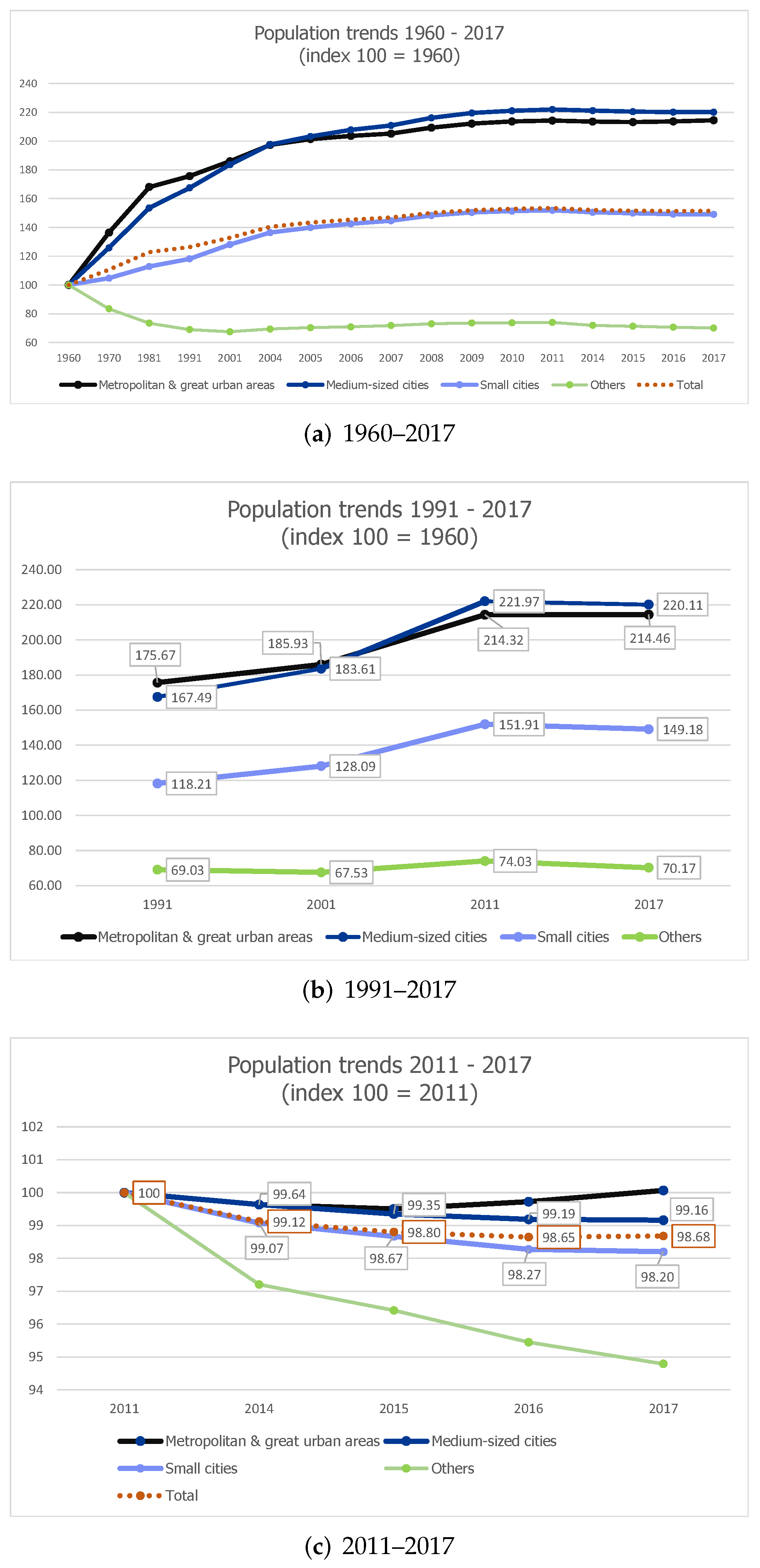
The Organization for Economic Cooperation and Development (OECD) has established a classification of those municipalities in connection with their membership to functional areas, which are economic units characterized by a densely inhabited city core and a commuting zone whose labor market is highly integrated with those cores [30]. Considering this approach, large metropolitan and metropolitan areas in Spain represent 10.0 percent (816) of the total number of municipalities, while medium-sized cities and small cities correspond to 5.4 percent (442). In terms of population, 54.4 percent (25,318,313 inhabitants) of the total population live in large metropolitan and metropolitan areas, while 15 percent (7,352,638 inhabitants) live in medium-sized cities and small cities. Up to 84.5 percent of municipalities (6866) are not included in these functional urban areas, which represent almost 30 percent of the total population (13,901,181 inhabitants). The locations of medium-sized cities and small cities are scattered across the territory, and they play an important role in terms of providing infrastructure and services to the population, including those municipalities not belonging to functional urban areas. However, in contrast to the need-based account that underlies the connection between the municipalities not belonging to functional areas and medium-sized and small cities, the population trends reveal that these categories have experienced a loss of population during the last decade (see Figure 1). Only large metropolitan and metropolitan areas during the last decade have had a slight increase in population.
3.2. Data
This study covers the entire Spanish territory (including the Canary and Balearic Islands, and the autonomous cities of Ceuta and Melilla) and focuses on the municipal level of data aggregation. At present, the Spanish territory is administratively represented by 8124 municipalities.
Firstly, this study did not apply the population size criteria to reduce the number of municipalities to be included in the dataset, nor the condition of population growth, stability, and loss. Compared to other studies [14], this model did not begin with a consideration of population loss as the main determinant for describing shrinkage. Consequently, all municipalities were initially considered in the model, and we only discarded those with data completeness and quality issues. The analysis of the results will provide some support in finding data patterns in municipalities, of either population growth, stability, or loss.
Moreover, this study provides a more comprehensive view of the multidimensional shrinkage phenomena by including a wider range of variables considered. These variables aim to cover the approach that existing research has applied in its study. Data gathering comprises a total of 36 variables that represent six dimensions: population change, demography, mobility, education, housing, and economy. In addition, this study is applied to the specific context of Spain and may easily be replicable in other territories since the variables considered were gathered and provided by the Spanish National Institute of Statistics. In the European context, the same variables were provided by the different national institutes of statistics, and in the international context, some countries provided similar variables. Another important boundary of the research is the determination of the reference period in which to implement this method. The study covers the last 30 years; it begins in 1991 and comprises the last three population and housing censuses available: 1991, 2001, and 2011. The decadal compilation of variables was retrieved from the Spanish National Statistical Institute (INE) and the Spanish Real Estate Cadastre data sources. Table 1 describes each of the variables collected, resulting in a 10-year data panel. Since it is assumed that there is a time lag for the different variables to influence the population change, we defined the compound annual growth rate (CAGR) considering a 10-year lapse. This means that for 1991, we considered the population change derived from the period of 2001–1991; for 2001, the population change was calculated considering the period of 2011–2001; and for 2011, the CAGR value was calculated considering the 2020–2011 period.
When processing the data, we found multiple problems that could not be corrected, which then forced us to discard them. This reduced the number of analyzed municipalities to 3449. The main problem was the lack of values in one or more variables for many municipalities. The cause of the lacking data was the fact that the affected municipalities were small villages with a low number of people, and in these cases, the Spanish National Statistical Institute did not provide a complete dataset for reasons of confidentiality and sample representativeness, even if this information was required for research purposes. Although SOM may be forgiving to some extent with respect to missing data (by ignoring the missing dimensions when computing for model similarities), many of the affected municipalities lacked half or more of the variables, making them completely unusable for the analysis. We tried the option of including them in the analysis and discovered that they completely distorted the results. More specifically, their use created a SOM that was discontinuous and did not respect the data topology (similar data did not end in close clusters). Considering the gathered dataset, most of the municipalities that had been omitted from the study were small municipalities with less than 300 inhabitants not belonging to any functional area. This represented less than 5 percent of the total population.
Since SOM requires input data records with complete information, all incomplete data records were useless and had to be removed. Additionally, even though the lack of values did not affect the three records of a municipality (for the three corresponding dates), we found that the inclusion of municipalities not having complete data records for the three dates (1991, 2001, and 2011) produced undesirable effects in the analysis of the results. In particular, they generated discontinuities in the grouping of the SOM output nodes by the clusters, and these clusters could not be interpreted correctly. Our hypothesis about the reason for such behavior is that it was caused by data quality problems in those data from municipalities with incomplete information. For example, a deeper analysis of these records showed several variables at zero even though such a value is not possible in such features.
3.3. Methodology
A self-organizing map is an artificial neural network that performs a dimension reduction of the input features (i.e., the data records corresponding to the information on municipalities at a particular date) while preserving the topology of the input data. Figure 2 shows an example of a standard SOM architecture. Each input vector element is connected to the whole output feature map through a weight matrix that is obtained through training. The difference from other kinds of networks is that in the training, the weights are influenced by the neighboring neurons in the output topology. This can be used to produce a simple visualization of high-dimensional input data that would help to discover hidden non-linear structures in the data [31]. These models have been broadly used in the study of land transformation processes at all organizational levels [23,32,33,34]. However, to our knowledge, they have not been used on the population shrinking phenomena studied in this paper. Differently from other analysis approaches such as the use of PCA followed by k-means or hierarchical clustering, the use of a SOM model provides a clearer analysis in terms of relations between the obtained aggregations. The SOM model does not only aggregate resources by similarity, but it also allows for a visual interpretation of the results without the need for reducing the dimensions of the input data, as it has been performed in other approaches.
Our objective was to analyze the evolution of multiple variables for a 30-year period (the period that we have data on) in order to identify how these variables affect the shrinkage in Spain. This way, once they are identified, they can be used as predictors of the behavior of future changes. For this purpose, the self-organization maps (SOM) are a very suitable tool that provides a gradation in the aggregation of the studied municipalities in terms of their variables, which goes beyond simple clustering by population gain or loss. The bi-dimensional structure of the self-organization map provides a kind of “spatial” distribution of the analyzed data, showing the homogeneity or dispersion of the data around the different subsets of variables.
The use of SOM for the population analysis required the harmonization of the available input data so that they could be used as input for the neural network. Since the analyzed data included values from different years, they were affected by socio-political aspects that made them non-directly comparable. For instance, in Spain, the number of people with university degrees has been increasing continuously in the last forty years. Consequently, if the data were not adjusted to remove this influence, there would be a strong correlation between this variable and the year of the data. This would cause any aggregation model to end producing quasi perfect clusters by year. In order to remove the temporal effect in the variables of the data records associated with each year, we replaced the value of each variable with the result of the subtraction of the mean of the variable in that year. In addition, the resulting values for each variable were scaled to the 0–1 range to facilitate the SOM training.
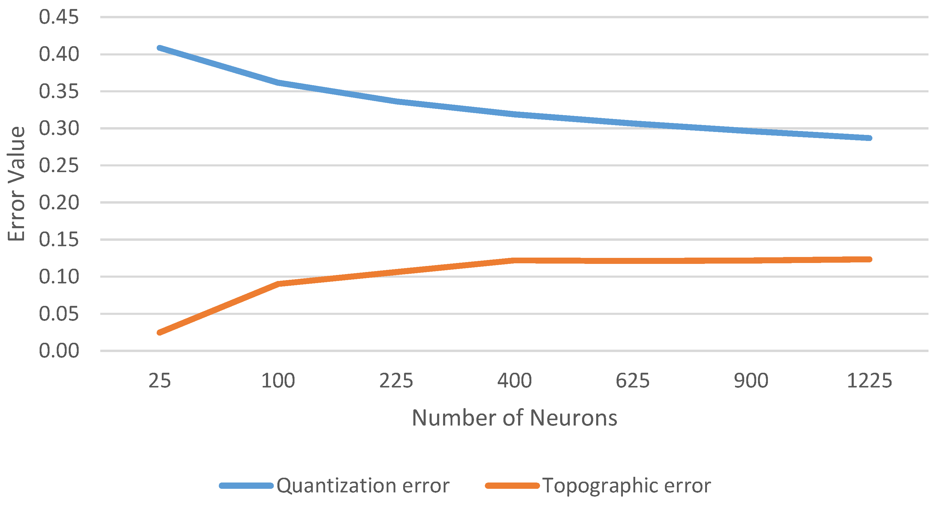
We used the SOM implementation provided by the SOM toolbox of Matlab 2019. Such toolbox simplifies the definition, training, and visualization of the self-organizing map, allowing us to focus on data analysis and interpretation. For the training of any SOM, a vital aspect is the parametrization of its structure, the dimensions, the distance function, and the training process. The selection of all these parameters was performed by sweeping along their value ranges and comparing the results obtained in terms of quantization and topographic error [35,36].
The quantization error (QE) measures the mean error of the input data with respect to the weights (W) of their assigned neuron (N) (see Equation (1)). This error tends to decrease with bigger dimensions of the output map because with more neurons, the data have more space to be distributed, and therefore the neuron weights can be closer to the assigned data. However, in a network of a given size, it is useful to compare the rest of the parameters.
The topographic error (TE) measures the distortion in the network topology. It is measured as the percentage of the input data that do not have the two best neuron candidates directly connected in the network (see Equation (2)). That is, it measures how well the SOM training has been able to assign similar data to adjacent neurons. This shows the suitability of the horizontal planes for clustering analysis. If the neuron assigned to an input element is far from the second best neuron (the one to which it would be assigned if the best one did not exist), it implies a distortion in the trained model. A high topographic error disables the possibility of inferring patterns from the movement of the data across the neuron topology because the defined topology is folded. Smaller networks tend to have smaller topographic errors because the data are compacted in the network neurons, but the generated results provide less information about the changes of variables in the horizontal planes of the network. In general, it is recommended that the number of neurons must be smaller than the input collection size to be able to provide a data clustering functionality of similar inputs. On the other hand, the size must be big enough to allow the component planes to show the longitudinal changes between inputs of different dates and identify the partial and non-lineal correlations between the input features [37].
There is no consensus regarding how to select the best network dimensions for a given dataset because it depends on the degree of the desired aggregation of the input data. Whereas large maps produce smaller and compact clusters, smaller ones generalize better. Vesanto and Alhoniemi [38] recommend that the number of neurons must be close to . As an alternative, Hasan and Shamsuddin [39] use the biggest eigenvalues of the data to set the network dimensions because they indicate the way the data are distributed when flattened. Other heuristics recommend to use a configuration with a small set of empty neurons (5–10%, or select a size ten times bigger than the desired number of clusters. We adopted the solution of Kohonen [40], who suggest to try multiple sizes and select from those with sufficient resolution and accuracy for the desired purpose. We tested a broad range of dimensions from 40 (supposing we wanted 4 clusters as minimum) to more than 676 neurons (which corresponded with of our original data). Figure 3 shows a summary of the evolution of the errors according to the number of neurons. It can be observed how the topographic error reaches a plateau when the size is increased. In contrast, the quantitative error continues to decrease with an increasing number of neurons, although this decrease is slower than the increasing number of neurons.
The connection structure of the SOM, the neighbor distance, and the distance function used to update the neuron weight are other important parameters that greatly affect SOM performance. They are quite dependent on the input data. Therefore, we tested all the combinations for the different network sizes in order to identify the configuration with the best performance. After analyzing the quality measures of the different parameter configurations, we selected: a SOM with 20 × 32 neurons; a hexagonal structure; the Euclidean distance to assign the data to the neurons; and a neighborhood distance of 3 steps (when updating the weights of a neuron, all with a distance of 3 in the SOM topology are also updated). The selected values produced a SOM without discontinuities, and it separated the source data enough to allow us to identify patterns in them. In addition, we can also observe in Figure 3 that with an increasing size of neurons (with respect to our chosen size), the quantization error slowly decreases.
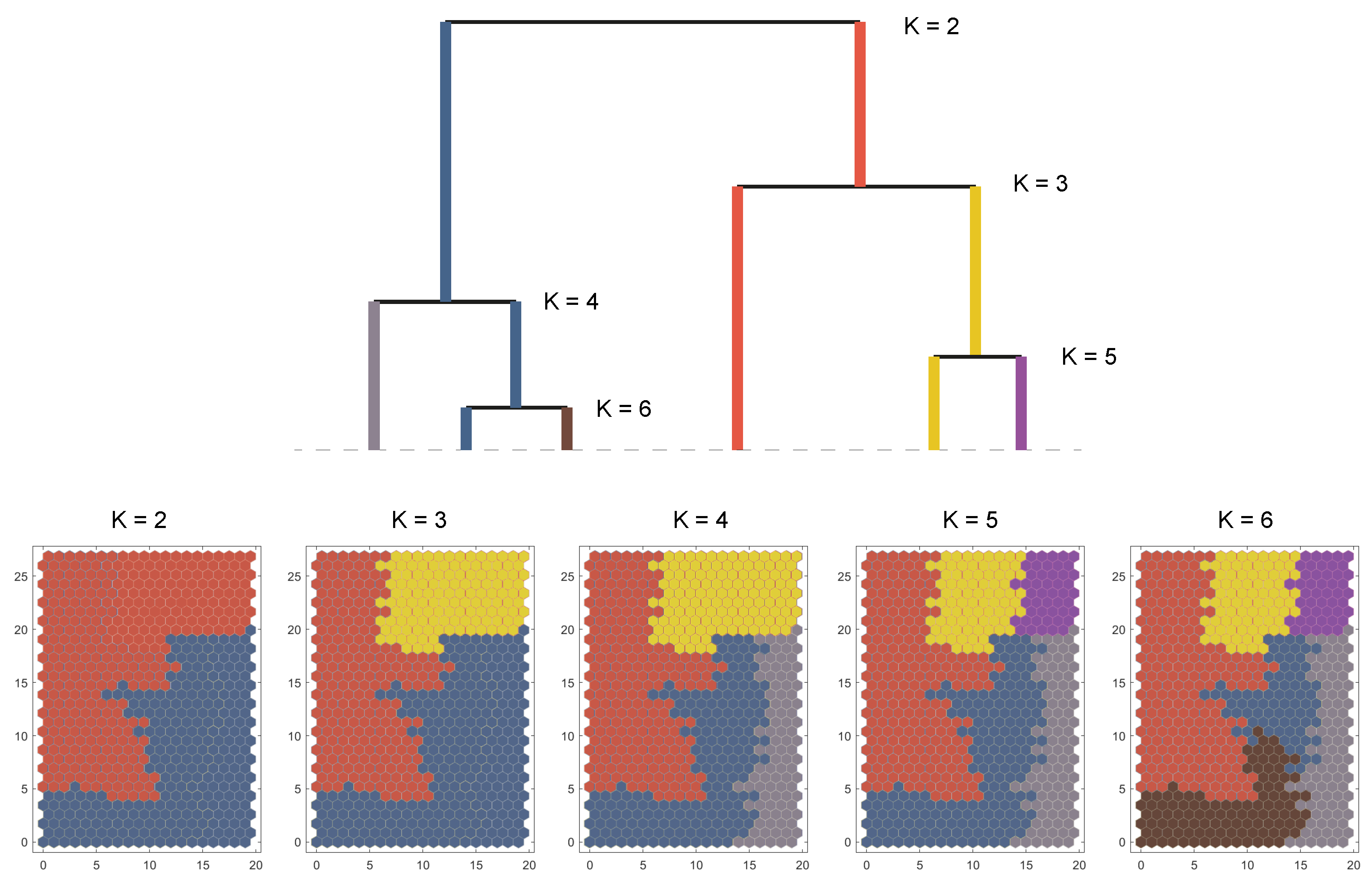
The SOM model provides data classification that allows for the analysis of the input data structure and the identification of hidden partial correlations between the data. However, a high number of neurons implies a high number of classification categories, which makes it difficult to have a clear overview of the data. To identify high-level relations between the neurons (that is, to find groups of neurons whose content share a common behavior with respect to shrinkage), we clustered their weights using the Ward algorithm [41]. This generated a dendrogram of the neurons, which facilitated the identification of the most suitable number of clusters in the SOM. Using this suitable number of clusters, we were able to distribute the output nodes (neurons) of the output SOM map in homogeneous areas (clusters) representing different types of municipalities.
The last step of the methodology is the identification of the longitudinal trajectories of the municipalities through time via the different nodes and clusters of the SOM output map. For each cluster, we considered the fact that it is important to identify the remain trajectories, the moved into trajectories, and the moved out trajectories. With remain trajectories, we mean the directed paths followed by the municipalities that started and ended in the same cluster during the studied period. The moved into trajectories refer to the trajectories followed by the municipalities that started the studied period in a cluster different from that to which the municipality belonged at the end of the period. Similarly, the moved out trajectories refer to the trajectories followed by the municipalities that ended the studied period in a cluster different from the cluster to which the municipality belonged at the beginning of the period. Algorithm 1 shows the algorithm that we designed to identify these three trajectories for each cluster. The functions and check if a pair is the end of a remain trajectory or the end of a moved into trajectory, respectively. In the same way, checks if a pair is the beginning of a moved out trajectory. Last, the function generates the trajectory associated with a municipality. This trajectory is a directed path that consists of the arcs defining the movement of a municipality along two consecutive dates analyzed in the studied period.
| Algorithm 1: Generation of longitudinal trajectories |
 |
4. Results
4.1. Feature Weights and Component Planes
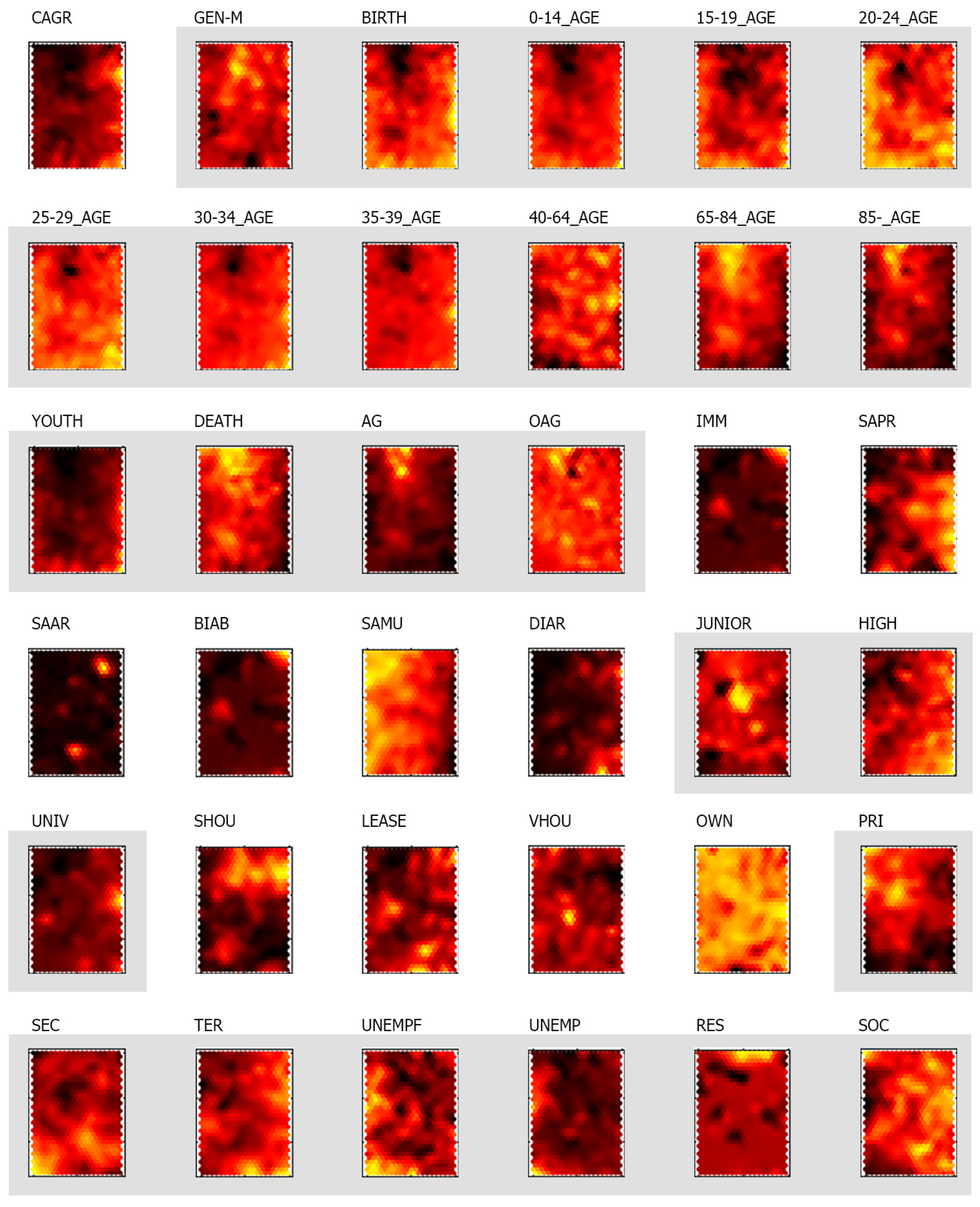
Figure 4 shows one of the main outputs of the SOM technique: the set of component planes graphically showing the values of the 36 variables that were considered for the distribution of the municipalities along the SOM map nodes. This can be considered as a first approach to understanding the non-linear correlations between the values of variables.
In Figure 4, high scores are depicted in yellow, and low ones are in black. Some variables such as the birth rate, the mobility within the province and the region, the rates of graduates from high school and university, the average socio-economic condition, or the tertiary industrial activity reveal high scores towards the right side of the planes, descending towards low scores on the left side of the planes.
Conversely, some other variables such as mobility within the same municipality and the primary industrial activity reveal an opposite pattern of high scores towards the top-left side of the planes.
Partial correlations are also identified. For instance, the secondary industrial activity has a more concentrated pattern of high scores towards the bottom-left side of the planes. In the case of the population between 65 and 84, the population over 85 years old, and the death rate, the higher values are associated with the top side of the planes. The restoration activity, a variable commonly associated with low shrinkage values, has a concentrated pattern of high levels towards the top-center side of the planes.
With respect to the residential (housing) variables, owning a house does not reveal a pattern where shrinkage may be characterized because this variable presents high values almost homogeneously distributed along the plane. Conversely, second housing appears as a variable associated with high values in some specific locations on the planes.
Finally, the population loss (CAGR) does not depict a high variance value and high scores concentrate towards the right side of the planes.
4.2. Cluster Characterization and Geographic Distribution of Shrinkage
As indicated in Section 3.3, we used a clustering algorithm to define the homogeneous regions of the SOM output space with similar characteristics. Figure 5 shows a dendrogram of the SOM neurons, together with the clusters generated according to the number of selected clusters. This analysis of alternatives has allowed us to select as the most appropriate number of clusters to be able to characterize with sufficient detail the types of municipalities in relation to its shrinkage behavior.
In addition, to better understand the features of the four clusters, Table 2 reports the mean values of the variables in the nodes contained in these clusters. Because the difference in magnitude between the obtained values is not intuitive, we studied the variables that better defined each of the clusters by calculating the variance between the means of each variable. Taking into account Table 2 and the previous analysis of component planes, we were able to obtain a qualitative description of the four clusters. For the population variations, this study considered the shrinking threshold value of at least 1 percent per year [5]. Considering this value, the study identified three categories for the variable CAGR: positive (), stagnant (), and negative (). Cluster 1 contains municipalities with population and activity growth that have no risk of starting a shrinkage path soon. Cluster 2 reveals stable areas in terms of population and economic activity, but those placed in specific areas of the cluster show signs of the start of a declining path. Cluster 3 shows areas with a clear decline of population and economic activity. Finally, Cluster 4 aggregates municipalities showing a change of economic activity. They mainly cover areas where tourism has become the main economic factor, replacing the original activities. The details of these clusters are as follows:
- Cluster 1 (low shrinkage, positive CAGR: 0.026): The municipalities in this cluster reveal high values with respect to the birth rate, the youth index, the percentage of people in their thirties, the percentage of people who graduated from high school and university, the socioeconomic condition, and the tertiary activity rate. In addition, this cluster holds the highest percentage of people living in a province or region different from the one corresponding to their birth place (SAPR and DIAR). Last, this cluster shows low values with respect to the aging index, the death index, the unemployment rate, and the primary activity rate.
- Cluster 2 (middle shrinkage, stagnant CAGR: 0.007): This cluster holds median values with respect to the birth rate, the youth index, the percentage of people living in the same province as the one corresponding to their birth place, the aging index, and the death index. The cluster is also characterized by low values regarding the percentage of foreign people and the lowest values for the second housing rate. Last, this cluster shows average socioeconomic condition scores slightly lower than those of other clusters (specially for cluster 1 and 4), and high secondary activity and unemployment rates.
- Cluster 3 (high shrinkage, negative CAGR: −0.010): This cluster holds low values with respect to the birth rate and the youth index. In addition, the cluster has the lowest values regarding the restoration activity, the socioeconomic condition, the leased housing rates, and the percentage of people who graduated from high school and university. On the contrary, this cluster is characterized by the highest values with respect to the primary activity, the unemployment rate for people who are looking for their first employment, and the percentage of people living in the same municipality as their birth place. Last, the cluster also shows high values for the death rate and the aging index.
- Cluster 4 (middle shrinkage, stagnant CAGR: 0.001): This cluster is characterized by the lowest values of the birth rate and the youth index. It also has the lowest values regarding the vacant housing and the unemployment rates. In addition, the cluster holds median values with respect to the tertiary activity (similar to cluster 2). Last, it must be noted that this cluster holds the highest values concerning the death rate, the aging index, the percentage of foreign people, the secondary housing rate, the restoration activity, and the percentage of people living in the same region as the one corresponding to their birth place.
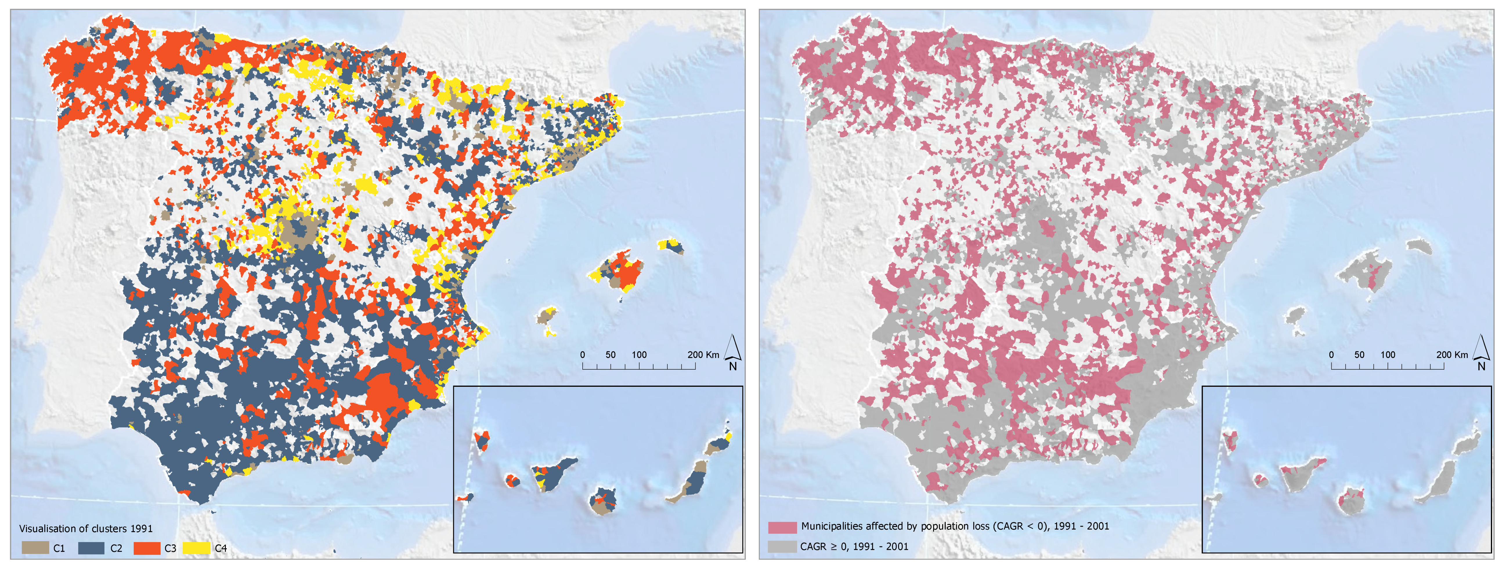
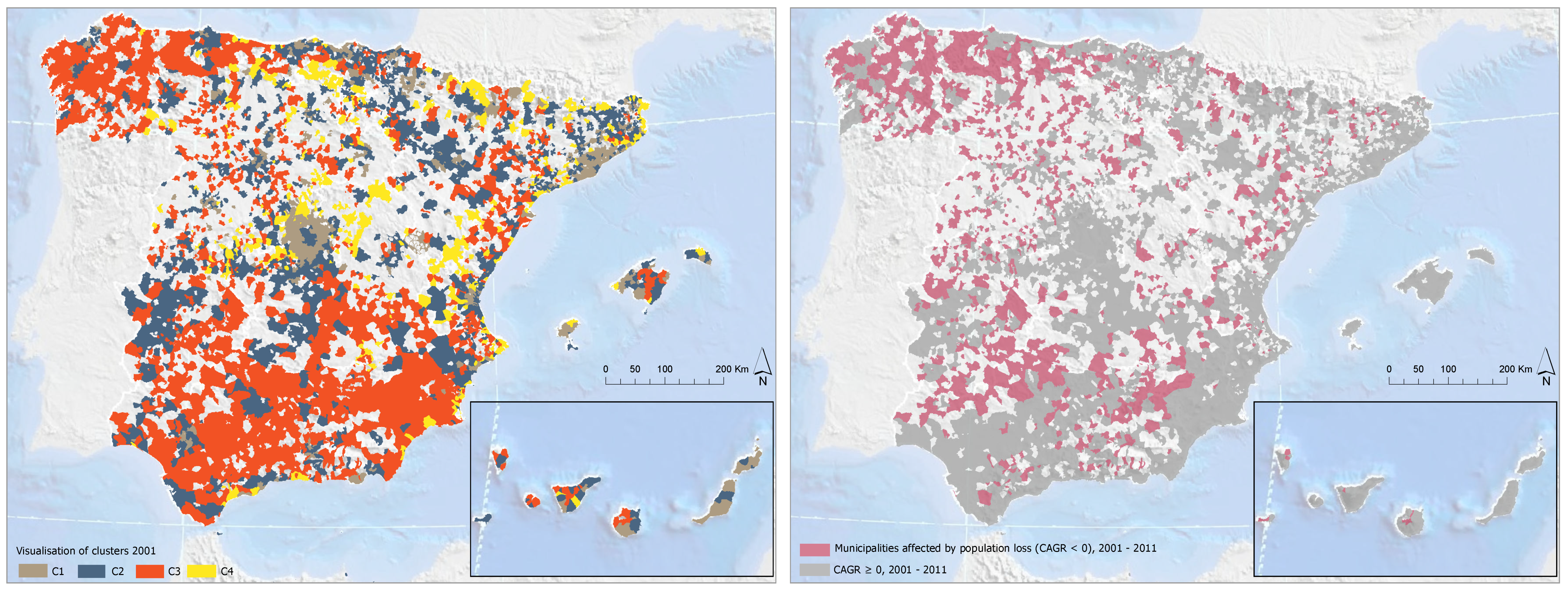
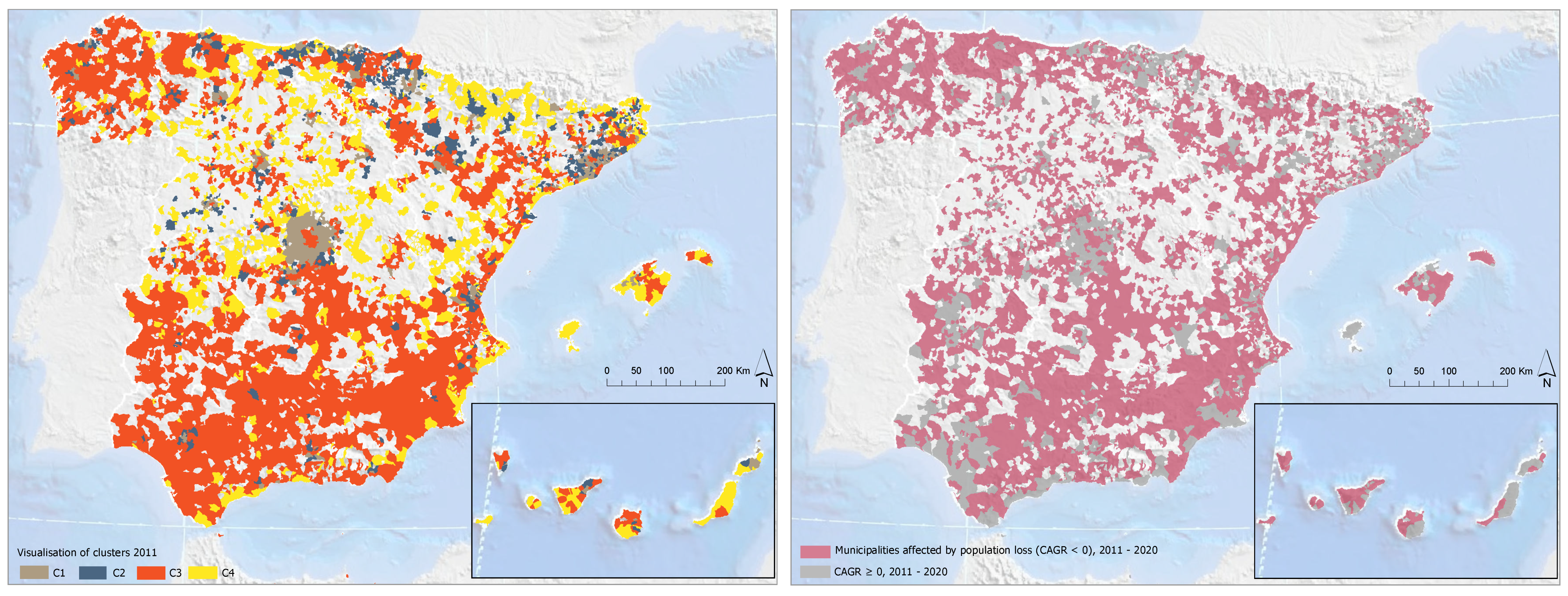
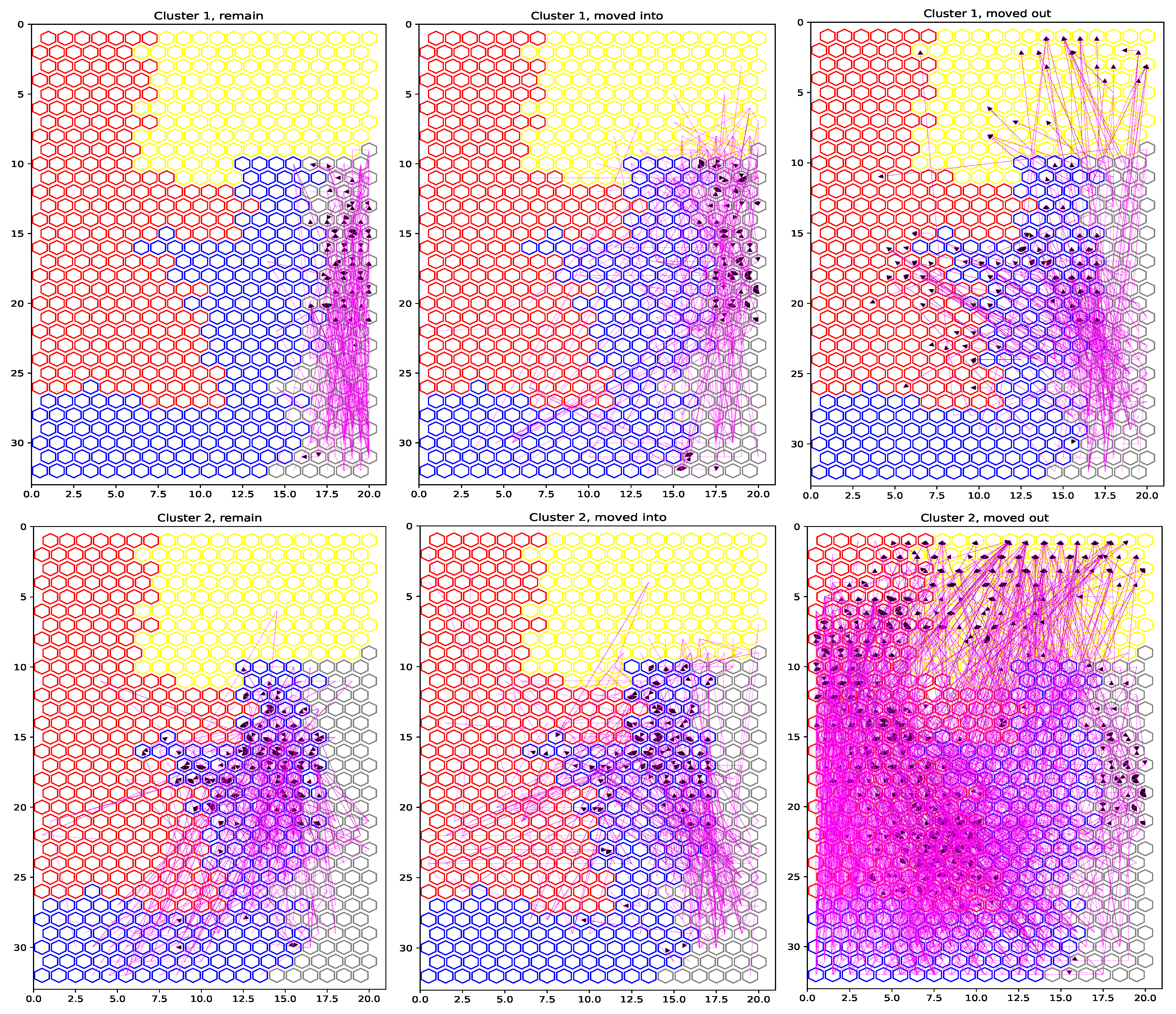
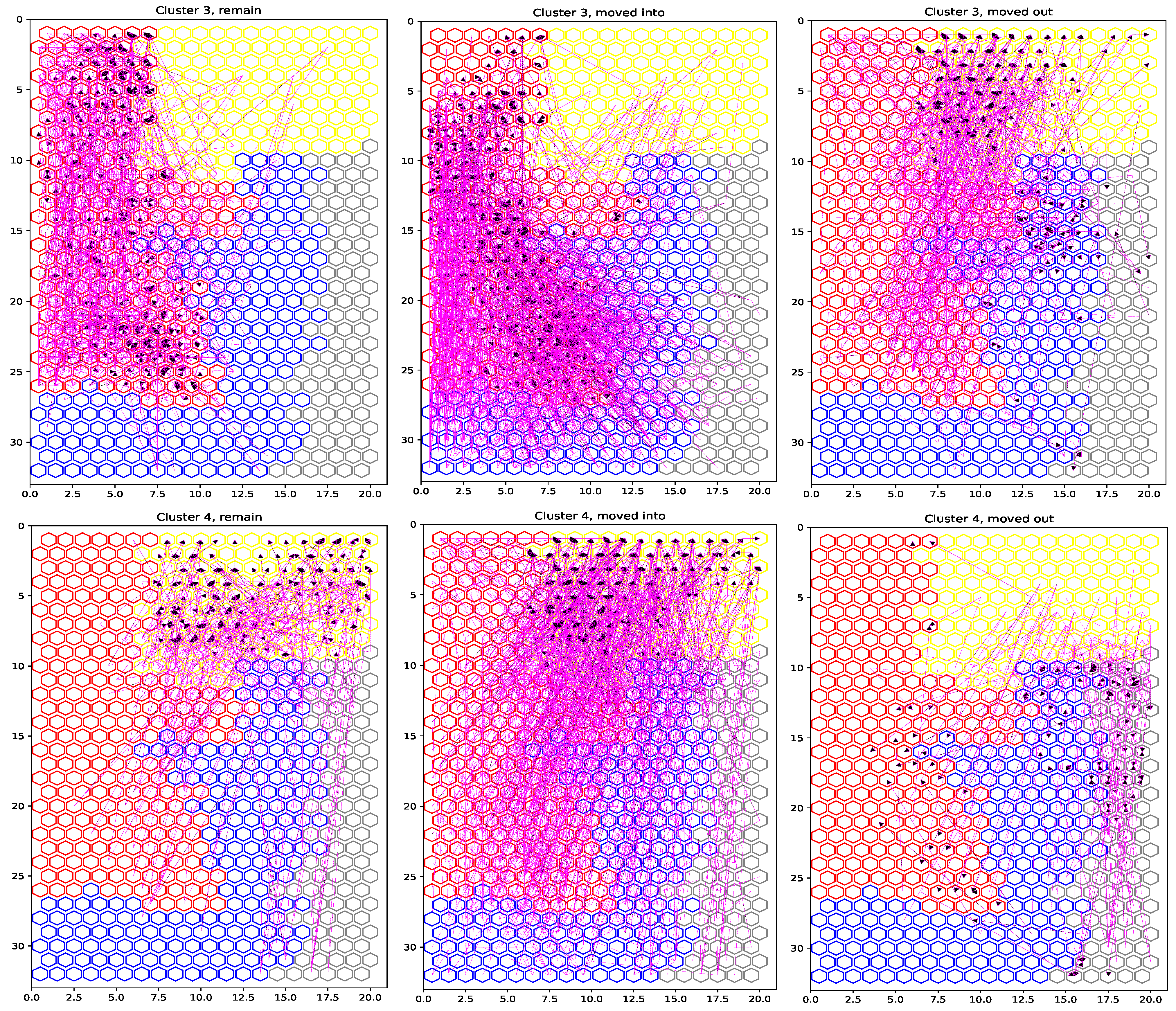
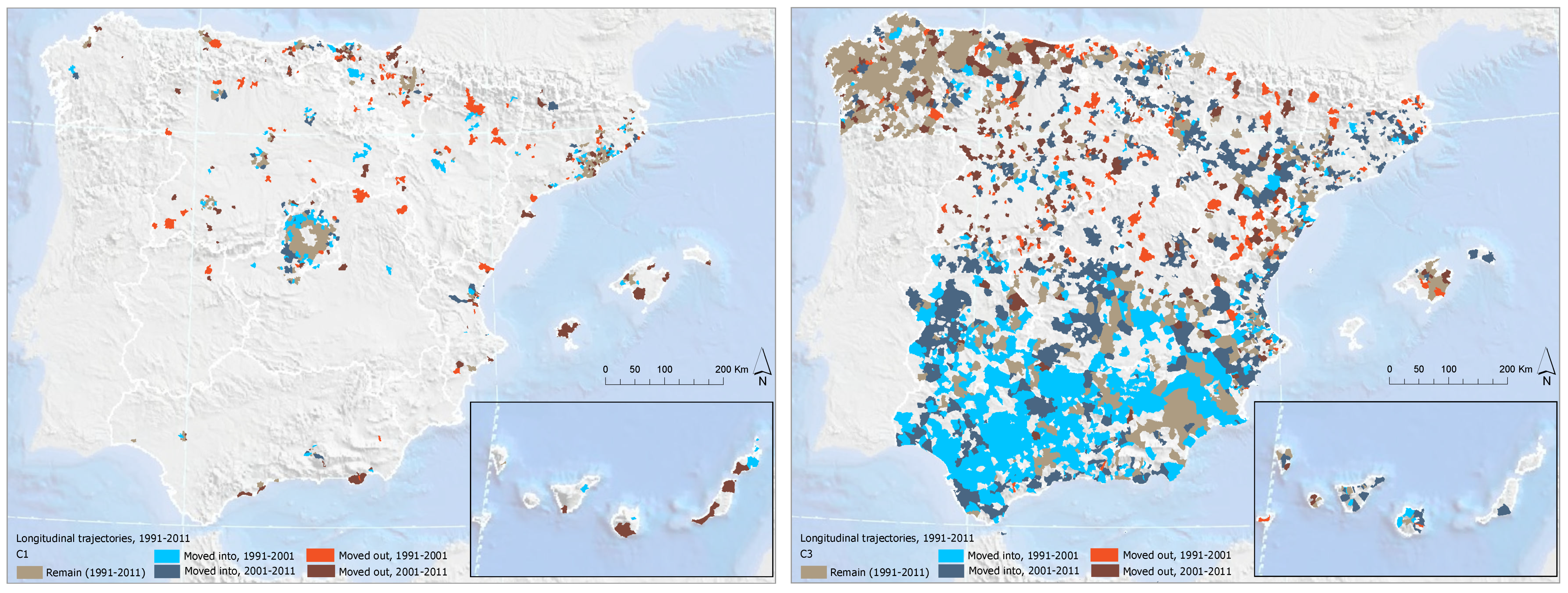
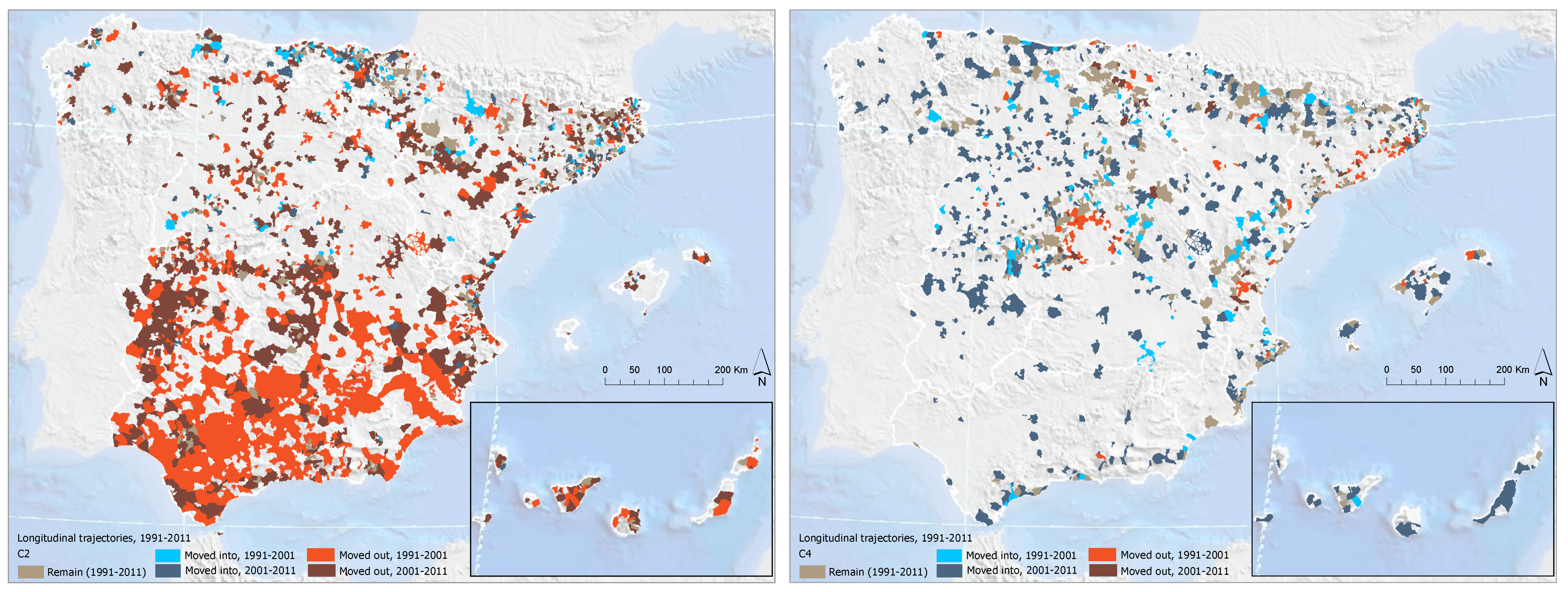
The correspondence with the specific territories affected by this characterization of shrinkage is depicted in Figure A1, Figure A2 and Figure A3. It also outlines of the spatial correspondence between the clusters and the areas affected by population loss during the three considered decades. Moreover, the partnership between the horizontal trajectories of municipalities and their geographical distribution, shown in Figure A4, Figure A5, Figure A6 and Figure A7, provides evidence of some interesting dynamics that help to characterize the shrinkage phenomenon over the last decades. On the one hand, Figure A4 and Figure A5 show three SOM maps for each cluster remarking: a first map with nodes where municipalities remain during the three decades; a second map with arcs linking the nodes of municipalities that moved into the cluster nodes in 2001 or 2011; and a third map with arcs linking the nodes of the municipalities that moved out from the cluster in 2001 or 2011. The arrow end points in black indicate the final location of the trajectories. On the other hand, Figure A6 and Figure A7 show the same information from a geographical perspective, using a geographical map for each cluster. Each map shows the area covered by the municipalities that belonged to the cluster in any of the three considered dates. Using different colors, we distinguish: the municipalities that remained in the cluster in all three dates (gray color); the municipalities that moved in in 2001 or 2011 (blue color); and the municipalities that moved out in 2001 or 2011 (red color).
Taking these trajectories into account, we must first remark that the municipalities that began in cluster 1 follow two distinct paths. The majority of municipalities belonging to Cluster 1 remain within the same cluster over time and have a geographical concentration, expanding from close to the center of the main cities (Madrid, Barcelona, Valencia, Zaragoza, Sevilla, Valladolid, Oviedo-Gijón, Santander) toward neighboring municipalities. This corresponds to areas where peripheralization may occur and constitute the hinterland of large functional areas. This path of improvement reinforces the definition of functional areas. Although the municipalities that followed this pattern were few, there is a clear path from the place where new municipalities moved into the cluster, particularly from the bottom side of Cluster 4, where the tertiary activity is high. The exception comes from municipalities that transitioned from Cluster 1 into Cluster 3 or 4, where a clear path of decline is revealed, specifically depicted by the population decrease in the last years.
Second, the municipalities that transitioned into Cluster 2 were few, but a great number of municipalities from Cluster 2 have transitioned into Cluster 3 (920 municipalities), and to a lesser extent, to Cluster 4 (257 municipalities). This also reveals a clear path of decline. The municipalities in this trajectory experienced a decrease in CAGR values and an increase in unemployment rate. Although the secondary activity rate is the highest of all the clusters considered, it decreases (naval, textile, wood, or furniture industry) during the two decades in favor of the tertiary activity sector. For instance, Avilés, La Coruña, Cartagena, or even the Ebro industrial corridor (Tudela, Gallur, Zaragoza, Pina, and Fuentes de Ebro). Typically, this refers to medium-sized cities. Additionally, it is important to consider the period in which this transition takes place, as Cluster 2 concludes the first decade of study with a decrease in the number of municipalities by 30 percent and the second decade with a decrease of more than 50 percent. The trajectories of the municipalities that moved from a starting position in Cluster 2 during the first decade define a path of decline located in geographic areas specifically in southern Spain; on the other hand, the trajectory during the last decade is distinct, increasing this transition along the Ebro, Duero, or Tajo rivers and Mediterranean coastal locations. This transition is characterized by higher levels of secondary housing rates and lower levels of mobility within the province.
Third, another path of decline is revealed when considering the trajectories of Clusters 3 and 4. They clearly depict the increase of the area, from a scattered to a merged pattern, in the last decade. Its trajectory, however, is different. While Cluster 3 increases the number of municipalities in more than 65 percent (from 925 to 1544 municipalities), Cluster 4 reaches an increase of more than 105 percent (from 469 to 965 municipalities) in the same considered period. Geographically, the trajectory in Cluster 3 reveals a considerable variability, mainly those municipalities showing movement from Cluster 2 towards 3 (920 municipalities). Indeed, this trajectory displays municipalities which started the decade in a different group and transitioned towards a pattern of decline. It represents municipalities which had turned from a reduction of mobility within the province (less commuting) in favor of the municipality, resulting from a decrease in population and tertiary activity rate during the last decade (Madrid or Zaragoza central areas).
Fourth, an important distinction arises when examining trajectories from Cluster 4, as it reveals that municipalities that transitioned into this group were lower in quantity than Cluster 3, but doubling the number of municipalities from Cluster 4 (from 469 to 965 municipalities) over the decades. Whereas only 230 municipalities remain in the same cluster during the studied period, the municipalities that moved into the cluster were originally from two different groups: Cluster 2 (223 municipalities) and Cluster 3 (273 municipalities). Indeed, most municipalities that exited Cluster 3 moved to Cluster 4, and they did mainly during the second decade (e.g., the touristic towns of Llanes or Ribadesella in the northern coast). The municipalities in Cluster 4 show higher values of secondary housing rate and restoration activity than those in Cluster 3, which is frequently explained in terms of tourist activity. A close inspection of the component planes for nodes within Cluster 4 reveals that these municipalities correspond to areas located in the coastal area (Balearic and Canary Islands, Llanes), close to natural parks (Ordesa y Monte Perdido, Doñana, Sierra Nevada, Sierra de Guadarrama, Picos de Europa), or in the outermost periphery of main cities (Barcelona, Madrid, or Valencia metropolitan areas).
This analysis shows that the generated model is able to explain how the different analyzed variables are connected to the shrinkage process. Each cluster obtained reflects a different shrinkage stage that ranges from prosperity to decline, and it is associated with specific ranges of the studied variables. Additionally, the use of the SOM model generates a gradation of the content in each cluster that is useful for identifying areas in the clusters whose content has a high tendency to move to other clusters. This means that the model is able to predict the evolution of shrinkage for future dates on the basis of the specific values of the studied variables.
5. Discussion
The existing research on shrinkage is focused on certain processes as determinants for this shrinkage. These processes are largely explained in terms of separate cause and effect, and their analysis specifically concerns territories affected by population loss. This approach receives empirical support from different case studies. Indeed, some studies target the influence of economic and demographic drivers on specific territories affected by shrinkage. While not disregarding the previous research, this study states the need for a perspective that takes into consideration the non-linear dynamics of shrinkage. Our work confirms that trajectories over a period of time can be drawn by combining factors that help to understand the interactions between different dimensions. With the proposal of a SOM-based method at the municipal level, we could detect data patterns that highlight the most relevant features and relations in the data. Our research confirms the identification of specific areas affected by shrinkage, which have already been explored from a local perspective by previous research in the field; an example is the work focused on Avilés [17], mainly using demographic data to explain shrinkage. In other words, local studies confirm that our results detect specific areas affected by shrinkage.
This study has also demonstrated that there is a correspondence between low shrinkage values in the hinterland of functional areas, and it is possible to distinguish between the absence of signs of a declining path in the hinterland and the signs of the declining path of core cities. This result may reflect the importance of medium-sized cities and small towns. They are extremely heterogeneous in terms of belonging or not to functional urban areas and their population trend. Further research should explore this condition of population size, urban areas, and local environment factors that have been of importance in the characterization of the clusters. Moreover, the longitudinal trajectories of shrinkage outline how municipalities move from one cluster to another across time (Figure A4, Figure A5, Figure A6 and Figure A7). It identifies how a specific municipality moves from a declining status to a growing one, or vice-versa.
In addition, this study finds that the clustering pattern depicted in the SOM output space reveals a diagonal trajectory between the municipalities belonging to Clusters 1 (bottom-right side of the plane) and the municipalities belonging to Cluster 3 (top left of the plane), which is clearly differentiated and characterized in terms of shrinkage.
The municipalities from Cluster 1 reveal low shrinkage. It is also supported that the municipal trajectory of those that join this cluster are only 5 percent of the total sample (177 municipalities) and are frequently located in neighboring municipalities of the main cities. Furthermore, this trajectory helps to reveal a path of peripheralization over the hinterland of large functional areas, which is associated mainly with demographic (birth rate), mobility (mainly within the region), and economic (tertiary industrial activity) and formative dimensions (graduated from high school and university). It is also interesting to note that the residential dimension (housing) representation in the target cluster provides evidence that the share of second, leased, owned, or vacant housing rate does not explain this association of municipalities in Cluster 1.
Conversely, the municipalities from Cluster 3 show high shrinkage. The trajectories to Cluster 3 reveal an important increase in the number of municipalities that end up in this cluster (1544 municipalities) and a clear transition from municipalities that moved from Cluster 2 (920 municipalities). Indeed, none of the municipalities that began in Cluster 2 and exited to move to group 3 followed paths of revitalization. Spatially, these municipalities have a much more geographical concentration, expanding southward and increasing their presence along the main rivers, possibly indicating the permanence of the primary activity rate. These municipalities also display a significant demographic stagnation (lower birth rate and youth index) as well as a low percentage of graduates from high school and universities. They represent municipalities which had long consolidated settlements resulting from the high presence of home-ownership and residents that are living in the same municipality they were born in.
In this study, we used a method to construct a predictive model and applied it to the entire Spanish territory. Since our work was based on its condition of exploratory data analysis, it considered a wider range of variables than previous holistic research studies [42]. Another interesting finding suggests that this exploratory method did not define a preliminary hypothesis to test, but it made possible the understanding of a prediction model for shrinkage scenarios. This approach has important implications for policy because it can allow municipalities to take advantage of the predictions of shrinkage. For example, Figure A4 and Figure A5 indicate the position in the SOM output space of those municipalities whose horizontal trajectory makes them more predisposed to change from one cluster to another. Thus, this means that municipalities from the bottom side of Cluster 1 are more likely to move out (and be affected by shrinkage dynamics) than other municipalities from the top side of Cluster 1. To the same extent, municipalities located on the top side of Cluster 4 are more likely to remain in the same cluster than those towards the bottom side of Cluster 4.
Although the international research on this topic has had little impact on the design of policy responses [43], when it comes to the improvement of the resilience of the territories with respect to shrinkage, it may be useful for a wider definition of comprehensive improvement actions. For instance, variables belonging to the mobility (SAMU, SAPR) and housing (SHOU) dimensions have great importance in determining the intensity and impact of shrinkage in certain regions (Table 2). The variance value of the variable weight means in the output nodes gives evidence that the role of CAGR (population change) in creating these clusters is not so prevalent as it may have been initially thought.
Indeed, our analysis provides a differentiation of shrinkage trajectories from the last three decades and may be helpful as a starting point for the implementation of measures to handle shrinkage, depending on the cluster classification. The findings are specific to Spain at the municipal level of aggregation. The gathered data include variables from the 1991, 2001, and 2011 censuses. The processing of data has required a harmonization of all the values considered to remove the temporal trends in the mean of each variable. This has been achieved by grouping the data by year and removing the mean of each group.
Our model did not consider the entire municipal universe. Because the analysis of results is limited to 3449 municipalities, we are unable to predict factors that may shape shrinkage patterns for all the municipalities. Since the Spanish National Census has not provided the complete dataset for reasons of confidentiality and sample representativeness, several municipalities have some missing data in one or more of the 36 features considered for the 1991, 2001, and 2011 censuses. Initially, the municipalities that were lacking some of these features were included in the analysis. However, when processing the data, the SOM output included certain discontinuities that were related to those municipalities with incomplete information, and as a result, those municipalities were removed from the analysis. Future research could examine the factors of shrinkage that determine trajectories of change at the municipal level of data aggregation from a comparative cross-national perspective.
6. Conclusions
This paper used a SOM-based model to detect data patterns related to the dynamics of shrinkage in the Spanish territory during the last three decades. This analysis demonstrated which patterns help to identify the characterization and geographic distribution of municipalities by evaluating their horizontal trajectory. This analysis demonstrated the factors that influence the shrinkage, the identification of trajectories of shrinkage, and a clustering of these trajectories. This study also predicted the shrinkage evolution of municipalities based on the specific values of the 36 studied variables. Policy implications would point to supporting the implementation of strategies, depending on the specifics of each obtained cluster. The proposed method considers the transitional change of local characteristics and the non-linear relations between all the considered determinants. To our knowledge, this is the first work applying the SOM technique to the study of the shrinkage phenomenon in Spain, and it has proved how some areas in the created SOM predict future shrinkage. In comparison with other related papers, we were able to identify specific areas in each cluster with higher probability for the remain, moved into, or moved out trajectories.
An important contribution of the paper is the process applied in order to populate and train the SOM model. Given that each data collection has its own particularities, the characteristics of the SOM must be adjusted for the desired purpose. In this context, we performed a comparison of multiple SOM configurations, together with the set-up of clustering parameters, in order to identify the configuration with the best performance for our use case. In addition, the experience obtained in our research allows for the consideration of data normalization issues such as the subtraction of the mean values of variables for each year to avoid the definition of annual clusters as it is commonly accomplished in other methods such as PCA or regression analysis models. Without this normalization, the generated SOM becomes biased, and the method does not work.
A final contribution of this work is the possibility of applying the same proposed methodology to study the shrinkage phenomenon in other countries using similar variables, since they have an equivalent national statistical dataset at the municipal level.
As future work, we would like to explore how data patterns help to understand the depiction of fragile areas over space and time, and how the variables of great importance in determining the impact of shrinkage differ depending on the spatial context represented by current functional urban areas.
Author Contributions
All the authors have participated in all the stages of the development of this work. All authors have read and agreed to the published version of the manuscript.
Funding
This work is part of the projects T59_20R and S04_20D supported by the Regional Government of Aragon (Spain), and the project PID2020-113353RB-I00 supported by the Spanish Ministry of Science and Innovation (MCIN/AEI/10.13039/501100011033/).
Institutional Review Board Statement
Not aplicable.
Informed Consent Statement
Not aplicable.
Data Availability Statement
The data and codes that support the findings of this study are available at figshare.com, with the link https://figshare.com/s/7f03b64d46ccd4b5185e (accessed on 18 January 2022).
Conflicts of Interest
The authors declare no conflict of interest.
Appendix A
Figure A1.
Maps showing the clusters of municipalities from a geographical perspective (part I).

Figure A2.
Maps showing the clusters of municipalities from a geographical perspective (part II).

Figure A3.
Maps showing the clusters of municipalities from a geographical perspective (part III).

Figure A4.
Visualization of longitudinal trajectories (part I). Cluster 1 is represented in gray; Cluster 2 in blue; Cluster 3 in red; and Cluster 4 in yellow.
Figure A4.
Visualization of longitudinal trajectories (part I). Cluster 1 is represented in gray; Cluster 2 in blue; Cluster 3 in red; and Cluster 4 in yellow.

Figure A5.
Visualization of longitudinal trajectories (part II). Cluster 1 is represented in gray; Cluster 2 in blue; Cluster 3 in red; and Cluster 4 in yellow.
Figure A5.
Visualization of longitudinal trajectories (part II). Cluster 1 is represented in gray; Cluster 2 in blue; Cluster 3 in red; and Cluster 4 in yellow.

Figure A6.
Visualization of longitudinal trajectories from a geographical perspective (part I).

Figure A7.
Visualization of longitudinal trajectories from a geographical perspective (part II).

References
- Beauregard, R.A. Urban Population Loss in Historical Perspective: United States, 1820–2000. Environ. Plan. A Econ. Space 2009, 41, 514–528. [Google Scholar] [CrossRef]
- Großmann, K.; Bontje, M.; Haase, A.; Mykhnenko, V. Shrinking cities: Notes for the further research agenda. Cities 2013, 35, 221–225. [Google Scholar] [CrossRef]
- Pallagst, K. Shrinking Cities; Planning Challenges from an International Perspective. Urban Infill Themenh.—Cities Grow. Smaller 2008, 10, 5–16. [Google Scholar]
- Du, Z.; Jin, L.; Ye, Y.; Zhang, H. Characteristics and influences of urban shrinkage in the exo-urbanization area of the Pearl River Delta, China. Cities 2020, 103, 102767. [Google Scholar] [CrossRef]
- Oswalt, P.; Rieniets, T.E. Atlas of Shrinking Cities; Hatje Cantz: Berlin, Germany, 2006. [Google Scholar]
- Martínez-Fernández, C.; Audirac, I.; Fol, S.; Cunningham-Sabot, E. Shrinking Cities: Urban Challenges of Globalization. Int. J. Urban Reg. Res. 2012, 36, 213–225. [Google Scholar] [CrossRef] [PubMed]
- Alves, D.; Barreira, A.P.; Guimarães, M.H.; Panagopoulos, T. Historical trajectories of currently shrinking Portuguese cities: A typology of urban shrinkage. Cities 2016, 52, 20–29. [Google Scholar] [CrossRef] [Green Version]
- Hattori, K.; Kaido, K.; Matsuyuki, M. The development of urban shrinkage discourse and policy response in Japan. Cities 2017, 69, 124–132. [Google Scholar] [CrossRef]
- Musterd, S.; Bontje, M. Understanding shrinkage in European regions. Built Environ. 2012, 38, 196–213. [Google Scholar]
- Haase, A.; Rink, D.; Grossmann, K.; Bernt, M.; Mykhnenko, V. Conceptualizing Urban Shrinkage. Environ. Plan. A Econ. Space 2014, 46, 1519–1534. [Google Scholar] [CrossRef] [Green Version]
- Turok, I.; Mykhnenko, V. The trajectories of European cities, 1960–2005. Cities 2007, 24, 165–182. [Google Scholar] [CrossRef]
- Wolff, M.; Haase, D.; Haase, A. Compact or spread? A quantitative spatial model of urban areas in Europe since 1990. PLoS ONE 2018, 13, e0192326. [Google Scholar] [CrossRef] [PubMed]
- Wolff, M.; Fol, S.; Roth, H.; Cunningham-Sabot, E. Shrinking cities: Measuring the phenomenon in France. Cybergeo Eur. J. Geogr. 2017. [Google Scholar] [CrossRef]
- Wolff, M.; Wiechmann, T. Urban growth and decline: Europe’s shrinking cities in a comparative perspective 1990–2010. Eur. Urban Reg. Stud. 2018, 25, 122–139. [Google Scholar] [CrossRef]
- Li, H.; Lo, K.; Zhang, P. Population shrinkage in resource-dependent cities in China: Processes, patterns and drivers. Chin. Geogr. Sci. 2020, 30, 1–15. [Google Scholar] [CrossRef] [Green Version]
- Segers, T.; Devisch, O.; Herssens, J.; Vanrie, J. Conceptualizing demographic shrinkage in a growing region—Creating opportunities for spatial practice. Landsc. Urban Plan. 2020, 195, 103711. [Google Scholar] [CrossRef]
- Sánchez-Moral, S.; Méndez, R.; Prada, J. El fenómeno de las ’shrinking cities’ en España: Una aproximación a las causas, efectos y estrategias de revitalización a través del caso de estudio de Avilés. In New Trends in the XXIst Century Spanish Geography. Contribución española al 32º Congreso de la Unión Geográfica Internacional; Raitt, D.I., Ed.; International Geographical Union: Cologne, Germany, 2012; pp. 252–266. [Google Scholar]
- Kohonen, T. Self-Organizing Maps; Springer Science & Business Media: Berlin/Heidelberg, Germany, 2012; Volume 30. [Google Scholar]
- Hewitson, B.C. Climate analysis, modelling, and regional downscaling using self-organizing maps. In Self-Organising Maps: Applications in Geographic Information Science; Agarwal, P., Skupin, A., Eds.; Wiley: Hoboken, NJ, USA, 2008; pp. 137–163. [Google Scholar]
- Li, T.; Sun, G.; Yang, C.; Liang, K.; Ma, S.; Huang, L. Using self-organizing map for coastal water quality classification: Towards a better understanding of patterns and processes. Sci. Total Environ. 2018, 628, 1446–1459. [Google Scholar] [CrossRef] [PubMed]
- Skupin, A.; Hagelman, R. Visualizing demographic trajectories with self-organizing maps. GeoInformatica 2005, 9, 159–179. [Google Scholar] [CrossRef]
- Henriques, R.; Bação, F.; Lobo, V. Carto-SOM: Cartogram creation using self-organizing maps. Int. J. Geogr. Inf. Sci. 2009, 23, 483–511. [Google Scholar] [CrossRef]
- Andrienko, G.; Andrienko, N.; Demsar, U.; Dransch, D.; Dykes, J.; Fabrikant, S.I.; Jern, M.; Kraak, M.J.; Schumann, H.; Tominski, C. Space, time and visual analytics. Int. J. Geogr. Inf. Sci. 2010, 24, 1577–1600. [Google Scholar] [CrossRef] [Green Version]
- Henriques, R.; Bacao, F.; Lobo, V. Exploratory geospatial data analysis using the GeoSOM suite. Comput. Environ. Urban Syst. 2012, 36, 218–232. [Google Scholar] [CrossRef]
- Delmelle, E.; Thill, J.C.; Furuseth, O.; Ludden, T. Trajectories of multidimensional neighbourhood quality of life change. Urban Stud. 2013, 50, 923–941. [Google Scholar] [CrossRef]
- Hagenauer, J.; Helbich, M. Hierarchical self-organizing maps for clustering spatiotemporal data. Int. J. Geogr. Inf. Sci. 2013, 27, 2026–2042. [Google Scholar] [CrossRef]
- Zhu, G.; Wu, X.; Ge, J.; Liu, F.; Zhao, W.; Wu, C. Influence of mining activities on groundwater hydrochemistry and heavy metal migration using a self-organizing map (SOM). J. Clean. Prod. 2020, 257, 120664. [Google Scholar] [CrossRef]
- Kumar, N.; Rustum, R.; Shankar, V.; Adeloye, A.J. Self-organizing map estimator for the crop water stress index. Comput. Electron. Agric. 2021, 187, 106232. [Google Scholar] [CrossRef]
- World Bank. World Bank Open Data; Technical Report; World Bank: Washington, DC, USA, 2018. [Google Scholar]
- Dijkstra, L.; Poelman, H.; Veneri, P. The EU-OECD definition of a functional urban area. In OECD Regional Development Working Papers; OECD Publishing: Paris, France, 2019; Volume 11. [Google Scholar] [CrossRef]
- Agarwal, P.; Skupin, A. Self-Organising Maps: Applications in Geographic Information Science; John Wiley & Sons: Hoboken, NJ, USA, 2008. [Google Scholar]
- Arribas-Bel, D.; Schmidt, C.R. Self-organizing maps and the US urban spatial structure. Environ. Plan. B Plan. Des. 2013, 40, 362–371. [Google Scholar] [CrossRef]
- Delmelle, E.C.; Haslauer, E.; Prinz, T. Social satisfaction, commuting and neighborhoods. J. Transp. Geogr. 2013, 30, 110–116. [Google Scholar] [CrossRef]
- Gahegan, M.; Takatsuka, M.; Wheeler, M.; Hardisty, F. Introducing GeoVISTA Studio: An integrated suite of visualization and computational methods for exploration and knowledge construction in geography. Comput. Environ. Urban Syst. 2002, 26, 267–292. [Google Scholar] [CrossRef]
- Pölzlbauer, G. Survey and Comparison of Quality Measures for Self-Organizing Maps. In Proceedings of the 5th Workshop Data Analysis, Erice, Italy, 27 October–3 November 2004; Elfa Academic: Press, Slovakia, 2004; pp. 67–82. [Google Scholar]
- Breard, G.T. Evaluating self-Organizing Map Quality Measures as Convergence Criteria. Master’s Thesis, University of Rhode Island, Kingston, RI, USA, 2017. [Google Scholar]
- Vesanto, J.; Himberg, J.; Alhoniemi, E.; Parhankangas, J. SOM Toolbox for Matlab 5; Technical Report; Citeseer: Princeton, NJ, USA, 2000. [Google Scholar]
- Vesanto, J.; Alhoniemi, E. Clustering of the self-organizing map. IEEE Trans. Neural Netw. 2000, 11, 586–600. [Google Scholar] [CrossRef] [PubMed]
- Hasan, S.; Shamsuddin, S.M. Multistrategy self-organizing map learning for classification problems. Comput. Intell. Neurosci. 2011, 2011, 1–11. [Google Scholar] [CrossRef] [Green Version]
- Kohonen, T. MATLAB Implementations and Applications of the Self-Organizing Map; Unigrafia Oy: Helsinki, Finland, 2014. [Google Scholar]
- Batagelj, V. Generalized Ward and related clustering problems. In Classification and Related Methods of Data Analysis; Bock, H.H., Ed.; Elsevier: Amsterdam, The Netherlands, 1988; pp. 67–74. [Google Scholar]
- Wiechmann, T.; Wolff, M. Urban Shrinkage in a Spatial Perspective—Operationalization of Shrinking Cities in Europe 1990–2010. In Proceedings of the AESOP-ACSP Joint Congress, Dublin, Ireland, 15–19 July 2013. [Google Scholar]
- Nelle, A.; Großmann, K.; Haase, D.; Sigrun Kabisch, D.R.; Wolff, M. Urban shrinkage in Germany: An entangled web of conditions, debates and policies. Cities 2017, 66, 116–123. [Google Scholar] [CrossRef]
Figure 1.
Population trends in Spain considering the Functional Urban Areas classification.

Figure 2.
Example of SOM architecture.

Figure 3.
Comparison of quantization and topographic errors of SOMs with different numbers of networks.
Figure 3.
Comparison of quantization and topographic errors of SOMs with different numbers of networks.

Figure 4.
Component planes. High scores are depicted in yellow, and low ones are in black.

Figure 5.
Clustering definition by applying the Ward technique. In the case of , Cluster 1 is represented by the color gray; Cluster 2 in blue; Cluster 3 in red; and Cluster 4 in yellow.
Figure 5.
Clustering definition by applying the Ward technique. In the case of , Cluster 1 is represented by the color gray; Cluster 2 in blue; Cluster 3 in red; and Cluster 4 in yellow.


Table 1.
Considered variables for the characterization of shrinkage. Definition, description, and identifier code used. Source: Spanish National Institute of Statistics.
Table 1.
Considered variables for the characterization of shrinkage. Definition, description, and identifier code used. Source: Spanish National Institute of Statistics.
| Dimension | n | Label | Variable | Description |
|---|---|---|---|---|
| Population change | 1 | CAGR | Compound annual growth rate | e.g., |
| Demography | 2 | GEN-M | Gender | Male/total population |
| 3 | BIRTH | Birth rate | Number of births in a year with respect to total population | |
| 4 | 0–14_AGE | Age structure | Persons 14/total population | |
| 5 | 15–19_AGE | Persons 15–19/total population | ||
| 6 | 20–24_AGE | Persons 20–24/total population | ||
| 7 | 25–29_AGE | Persons 25–29/total population | ||
| 8 | 30–34_AGE | Persons 30–34/total population | ||
| 9 | 35–39_AGE | Persons 35–39/total population | ||
| 10 | 40–64_AGE | Persons 40–64/total population | ||
| 11 | 65–84_AGE | Persons 65–84/total population | ||
| 12 | 85–_AGE | Persons 85/total population | ||
| 13 | YOUTH | Youth index | Population under 15 years old/population over 65 years old | |
| 14 | DEATH | Death rate | Number of deaths in a year with respect to total population | |
| 15 | AG | Aging index | Population above 85 years old/0–19 population | |
| 16 | OAG | Over-aging index | Population above 85 years old/ population above 65 years old | |
| Mobility | 17 | IMM | Foreign immigrants | Persons/total population |
| 18 | SAPR | Living in the same province they were born in | Persons/total population | |
| 19 | SAAR | Living in the same autonomous regions they were born in | Persons/total population | |
| 20 | BIAB | Born abroad | Persons/total population | |
| 21 | SAMU | Living in the same municipality they were born in | Persons/total population | |
| 22 | DIAR | Living in a different autonomous region from where they were born | Persons/total population | |
| Education | 23 | JUNIOR | Graduate from elementary, junior high school | Graduated above 15 years old/persons above 15 years old |
| 24 | HIGH | Graduate from high school | Graduated above 15 years old/persons above 15 years old | |
| 25 | UNIV | Graduate from college, university | Graduated above 15 years old/persons above 15 years old | |
| Housing | 26 | SHOU | Second housing rate | Second housing/total housing |
| 27 | LEASE | Leased housing rate | Leased housing/total housing | |
| 28 | VHOU | Vacant housing rate | Vacant housing/total housing | |
| 29 | OWN | Owned housing rate | Household/total housing | |
| Economy | 30 | PRI | Primary industry rate | Persons above 15 years old in primary industry sector/persons above 15 years old |
| 31 | SEC | Secondary industry rate | Persons above 15 years old in secondary industry sector/persons above 15 years old | |
| 32 | TER | Tertiary industry rate | Persons above 15 years old in tertiary industry sector/persons above 15 years old | |
| 33 | UNEMPF | Unemployment (looking for first employment) | Unemployed persons above 15 years old/persons above 15 years old | |
| 34 | UNEMP | Unemployment | Unemployed persons above 15 years old/persons above 15 years old | |
| 35 | RES | Restoration activity | Persons above 15 years old in restoration activity/persons above 15 years old | |
| 36 | SOC | Average socioeconomic condition | Arithmetic mean of categorized values from qualitative occupation, activity, and professional situation variables |
Table 2.
Variable weight means in the output nodes, ordered by variance value.
| Variable | Variance | C1 (n = 92) | C2 (n = 190) | C3 (n = 228) | C4 (n = 130) |
|---|---|---|---|---|---|
| SAMU | 0.0270 | 0.2683 | 0.5046 | 0.6670 | 0.5097 |
| SHOU | 0.0259 | 0.1998 | 0.1834 | 0.2138 | 0.5199 |
| SAPR | 0.0154 | 0.5369 | 0.3771 | 0.2540 | 0.2997 |
| PRI | 0.0097 | 0.1539 | 0.1836 | 0.3586 | 0.3116 |
| TER | 0.0060 | 0.5693 | 0.4603 | 0.3793 | 0.4583 |
| x65_84_AGE | 0.0045 | 0.1765 | 0.2393 | 0.3038 | 0.3266 |
| DIAR | 0.0042 | 0.2568 | 0.1526 | 0.0997 | 0.1794 |
| 35_39_AGE | 0.0034 | 0.5028 | 0.4271 | 0.3826 | 0.3741 |
| SEC | 0.0031 | 0.3823 | 0.4567 | 0.3542 | 0.3266 |
| UNIV | 0.0029 | 0.3240 | 0.2406 | 0.1967 | 0.2250 |
| RES | 0.0025 | 0.3261 | 0.3240 | 0.3003 | 0.4160 |
| SOC | 0.0020 | 0.4599 | 0.3866 | 0.3543 | 0.4185 |
| BIRTH | 0.0011 | 0.1949 | 0.1646 | 0.1342 | 0.1177 |
| YOUTH | 0.0010 | 0.1198 | 0.0765 | 0.0537 | 0.0467 |
| JUNIOR | 0.0010 | 0.3575 | 0.3792 | 0.4161 | 0.4281 |
| HIGH | 0.0009 | 0.2887 | 0.2559 | 0.2140 | 0.2422 |
| VHOU | 0.0009 | 0.1622 | 0.1771 | 0.1957 | 0.1235 |
| 85-_AGE | 0.0006 | 0.0695 | 0.0938 | 0.1192 | 0.1261 |
| CAGR | 0.0004 | 0.3595 | 0.3266 | 0.3085 | 0.3214 |
| IMM | 0.0003 | 0.1364 | 0.1205 | 0.1159 | 0.1601 |
| BIAB | 0.0003 | 0.1511 | 0.1305 | 0.1250 | 0.1685 |
| UNEMP | 0.0003 | 0.2543 | 0.2711 | 0.2708 | 0.2293 |
| SAAR | 0.0003 | 0.0585 | 0.0685 | 0.0605 | 0.0982 |
| LEASE | 0.0003 | 0.1508 | 0.1473 | 0.1118 | 0.1333 |
| x15_19_AGE | 0.0002 | 0.1802 | 0.1756 | 0.1650 | 0.1458 |
| 0_14_AGE | 0.0002 | 0.0990 | 0.0889 | 0.0759 | 0.0649 |
| DEATH | 0.0001 | 0.0473 | 0.0627 | 0.0740 | 0.0761 |
| 20_24_AGE | 0.0001 | 0.2004 | 0.1996 | 0.1927 | 0.1721 |
| 30_34_AGE | 0.0001 | 0.1068 | 0.0925 | 0.0833 | 0.0788 |
| OWN | 0.0001 | 0.8108 | 0.7910 | 0.8184 | 0.8005 |
| 25_29_AGE | 0.0001 | 0.1353 | 0.1270 | 0.1195 | 0.1088 |
| GEN_M | 0.0001 | 0.4751 | 0.4718 | 0.4735 | 0.4951 |
| AG | 0.0000 | 0.0135 | 0.0181 | 0.0242 | 0.0330 |
| UNEMPF | 0.0000 | 0.0638 | 0.0721 | 0.0732 | 0.0555 |
| OAG | 0.0000 | 0.3370 | 0.3412 | 0.3478 | 0.3348 |
| 40_64_AGE | 0.0000 | 0.1995 | 0.1954 | 0.1969 | 0.2026 |
Publisher’s Note: MDPI stays neutral with regard to jurisdictional claims in published maps and institutional affiliations. |
© 2022 by the authors. Licensee MDPI, Basel, Switzerland. This article is an open access article distributed under the terms and conditions of the Creative Commons Attribution (CC BY) license (https://creativecommons.org/licenses/by/4.0/).
Share and Cite
MDPI and ACS Style
Ruiz-Varona, A.; Lacasta, J.; Nogueras-Iso, J. Self-Organizing Maps to Evaluate Multidimensional Trajectories of Shrinkage in Spain. ISPRS Int. J. Geo-Inf. 2022, 11, 77. https://doi.org/10.3390/ijgi11020077
AMA Style
Ruiz-Varona A, Lacasta J, Nogueras-Iso J. Self-Organizing Maps to Evaluate Multidimensional Trajectories of Shrinkage in Spain. ISPRS International Journal of Geo-Information. 2022; 11(2):77. https://doi.org/10.3390/ijgi11020077
Chicago/Turabian StyleRuiz-Varona, Ana, Javier Lacasta, and Javier Nogueras-Iso. 2022. "Self-Organizing Maps to Evaluate Multidimensional Trajectories of Shrinkage in Spain" ISPRS International Journal of Geo-Information 11, no. 2: 77. https://doi.org/10.3390/ijgi11020077
Note that from the first issue of 2016, this journal uses article numbers instead of page numbers. See further details here.