Integration of Web Processing Services with Workflow-Based Scientific Applications for Solving Environmental Monitoring Problems

Abstract

Nowadays, developing and applying advanced digital technologies for monitoring protected natural territories are critical problems. Collecting, digitalizing, storing, and analyzing spatiotemporal data on various aspects of the life cycle of such territories play a significant role in monitoring. Often, data processing requires the utilization of high-performance computing. To this end, the paper addresses a new approach to automation of implementing resource-intensive computational operations of web processing services in a heterogeneous distributed computing environment. To implement such an operation, we develop a workflow-based scientific application executed under the control of a multi-agent system. Agents represent heterogeneous resources of the environment and distribute the computational load among themselves. Software development is realized in the Orlando Tools framework, which we apply to creating and operating problem-oriented applications. The advantages of the proposed approach are in integrating geographic information services and high-performance computing tools, as well as in increasing computation speedup, balancing computational load, and improving the efficiency of resource use in the heterogeneous distributed computing environment. These advantages are shown in analyzing multidimensional time series.

1. Introduction

Nowadays, developing and applying advanced digital technologies for monitoring ecology and nature management of the environment (e.g., atmospheric air, surface land waters, sea waters, soil and land cover, landscapes, etc.) are critical for the scientific community [1]. In this context, protected natural territories deserve special attention and control due to the importance and uniqueness of their water, land, forest, biological, and other natural resources [2].

Generally, environmental monitoring is impossible without applying a multi-level information complex [3]. This complex is intended to consider and evaluate the cumulative anthropogenic effect from different impact sources to predict the possible response of natural environments and the evolution of their further state. The monitoring process includes determining locations and parameters of observation, selecting and placing sensors, receiving and transferring signals, processing and archiving data, visualizing information, supporting decision-making, etc. Geographic information systems (GISs) are integral structural elements of such complexes [4]. Moreover, development, publication, and assembling web services by research teams in various research fields based on open standards within an integrated GIS portal undoubtedly expand opportunities for interdisciplinary studies related to environmental monitoring [5]. When applying web services, end-users have access to distributed algorithms, models, data, and sensors for geodata processing.

However, due to the growth in the amount of information obtained and aggregated in the monitoring process, the modern development of GISs often requires big data analysis tools based on parallel and distributed computing [6,7]. Hence, specialists from different subject domains are faced with the need to solve problems of supercomputer engineering. In particular, the challenges in applying high-performance computing (HPC) when solving environmental monitoring problems are discussed by Lee et al. [8]. These authors suggest that while multiprocessor systems are the main elements of the computing environment, end-users should also use cloud and fog platforms. Cloud platforms provide flexible and dynamic provisioning additional resources on-demand. At the same time, fog platforms allow preprocessing data close to their sources. In such a heterogeneous computing environment, a non-trivial problem is ensuring efficient use of resources and computation speedup, as the number of consumed resources constantly increases. Thus, among the main challenges are the following:

• using resources of a distributed computing environment, in which heterogeneity is increasing every year, and interacting with local resource managers (LRMs) located in the nodes of resources [9],
• developing workflow-based applications, forming a composition of web services provided by different research projects, and executing workflows in a distributed computing environment, which necessitates making access to HPC resources more flexibly and straightforwardly [10],
• supporting a large spectrum of various open standards, such as the Open Cloud Computing Interface (OCCI) [11], Open Virtualization Format (OVF) [12], standards of the Open Source Geospatial Foundation (OSGeo) [13], and the Open Geospatial Consortium (OGC) [14],
• implementing other system operations, for example, computation scheduling and distribution of computational load respecting administrative policies of resource provisioning.

The efforts of many researchers are aimed at overcoming these challenges. Foerster et al. [15] suggest that the representation of data based on the OGC standards into mass-market geospatial applications increases the availability of information significantly, and is essential in practice for most end-users. For example, an open-source Java-based server, GeoServer, implements standard OGC protocols and provides end-users great flexibility in map creation and geospatial data sharing [16]. Among such standards are the Web Feature Service (WFS), Web Map Service (WMS), Web Coverage Service (WCS), Web Processing Service (WPS), and Web Map Tile Service (WMTS).

However, geospatial data should be timely and efficiently collected, aggregated, and transferred to GIS. Concerning big data, this requires high-performance data processing. Tools similar to such GISs are not addressed to these problems. Therefore, additional software, for example, tools for composition and management of WPS services, as well as virtualization and execution of grid or cloud computing, is required [17]. Owing to such a need, significant difficulties are created for both the providers of geographic information services and their end-users.

The workflow-based geoprocessing tool GeoJModelBuilder is considered in [18]. It is intended for integrating interoperable web sensors, geoprocessing services, and researcher’s models into workflows based on the OpenMI standard of OGC. When using this tool, it is often difficult to synchronize the modeled time when the models interact with each other. An approach to migrating of applications from a GIS portal to a private or public cloud is proposed in [19]. Wang et al. [20] represent the scalable implementation of atmospheric general circulation models on a multicore cluster when solving a problem of long-term simulations for climate change. Features of high-performance geocomputing on HPC clusters are discussed in [21].

Nevertheless, geospatial applications based on cloud computing technology still require further development [22]. Moreover, integration of HPC resources at diverse physical locations to execute a composite of web services developed by different researchers remains difficult within traditional workflow-based approaches [10]. One way to overcome this difficulty is proposed in [23]. Sun et al. present the Geoweaver system to improve efficiency in managing the full cycle of an artificial intelligence workflow.

Thus, owing to the uniqueness of each problem from a large spectrum of those solved with GISs, and the variety of software and hardware architectures used, as well as data sources and structures, the challenges have not been eliminated. In this regard, we contribute to this research field based on our practical experience in solving large-scale applied problems using parallel and distributed computing [24,25,26]. In this paper, we propose an approach integrating GIS portal capabilities and tools for creating problem-oriented, heterogeneous, distributed computing environments. Within the proposed approach, resource-intensive operations related to analyzing spatiotemporal data are implemented by the workflow-based application developed in the Orlando Tools (OT) framework [24] and represented by WPS services. The results are published on a GIS portal.

The rest of the paper is organized as follows. In Section 2, we represent a GIS portal used to support environmental monitoring of the protected Baikal natural territory and consider the capabilities of OT for developing and applying workflow-based scientific applications. Then, we propose an approach to automating the creation of WPS services as interfaces for workflows of the applications developed in OT. As an example of applying the proposed approach, a technique and tools for forecasting hourly air temperature are given in Section 3. In particular, adjusting the parameters of a prediction function (PF) is considered. This function is a multiextremal one. It has several adjusted parameters and generally requires parallel computing to find a global minimum. We provide a comprehensive analysis of computational experiments for adjusting the PF parameters and discuss the study results. Finally, Section 4 concludes the paper.

2. Proposed Approach: Methods and Tools

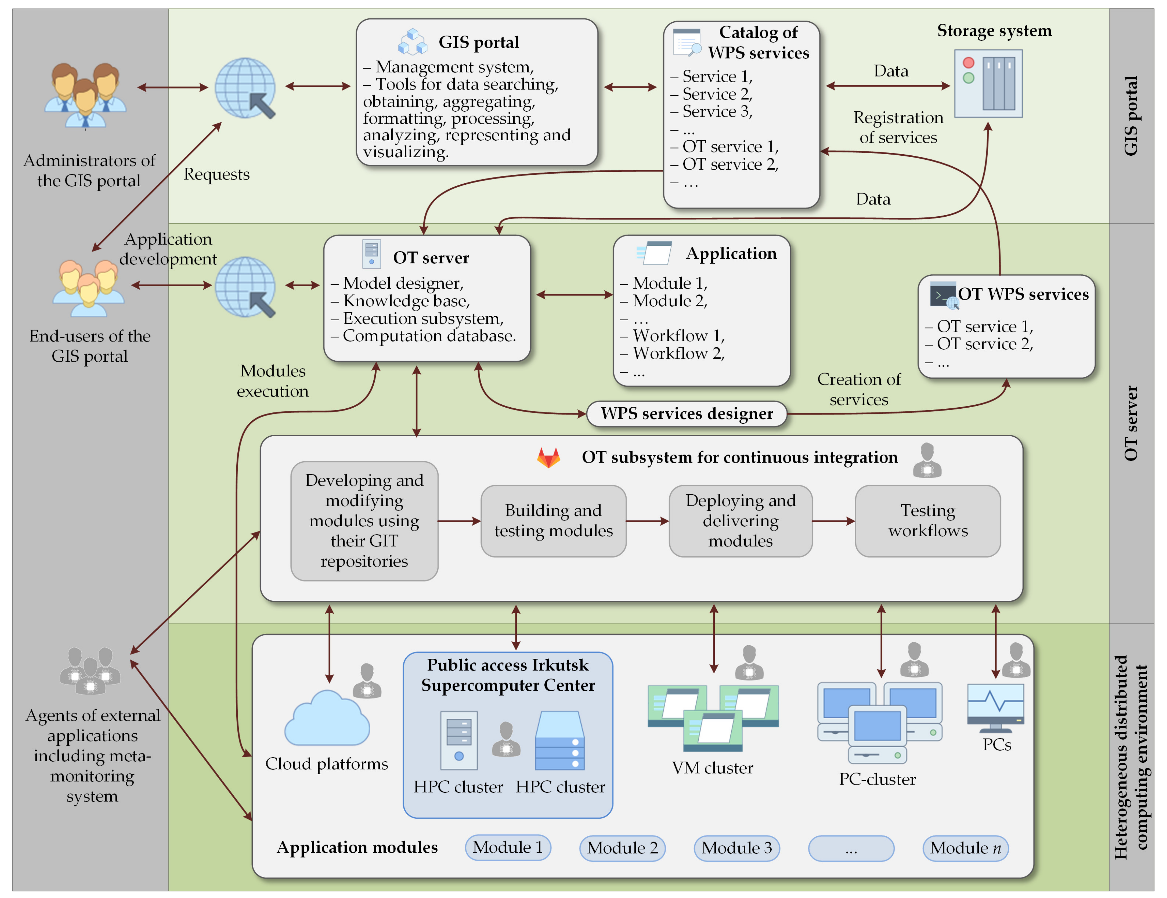
2.1. Automating Creation and Use of WPS Services within GIS Portal

A GIS portal of the Matrosov Institute for System Dynamics and Control Theory of the Siberian Branch of the Russian Academy of Sciences (ISDCT SB RAS) allows end-users to collect, process, and visualize their spatiotemporal data [27]. Spatiotemporal data map various geodata structures to specific locations in different periods. Within the GIS portal, its functionality is encapsulated into WPS services. The WPS specification describes a web service standard for publishing geoprocessing capabilities and provides an interface for processing spatiotemporal data. Data visualization is carried out with maps, tables, and diagrams.

The scheme for operating with spatiotemporal data is shown in Figure 1. Control and measuring equipment of weather stations, water level monitors, seismic vibrations detectors, satellites, and other monitoring systems collect, preprocess, and transfer information about the observed object states (observation results). These results (spatiotemporal data) are represented as data files, various databases, and different web services. The data meta-model determines the rules for searching, obtaining, aggregating, formatting, processing, representing, visualizing, and analyzing the data transmitted within the GIS portal.

For registered end-users, the web interface provides access to the functionality of the GIS portal. End-users can use the WPS services of other users or develop new services and register them in corresponding catalogs on the GIS portal. The database system provides each end-user with disk storage volumes to memorize the parameters of the launched services or their compositions. Access to storage is implemented through a web interface that enables end-users to upload and download data files. This storage service also provides a virtual file system on users’ personal computers (PCs). A management system supports interaction between the GIS portal components and their configuration.

Within the GIS portal, spatiotemporal data become available to different end-users in solving their practical and scientific problems. These data are widely used for updating topographic and navigational maps, agricultural monitoring, tracking the dynamics and state of forest felling, observing ice conditions, etc. For the last two decades, the GIS portal has been actively used in environmental monitoring of the protected Baikal natural territory.

We propose an approach to automating the execution of high-performance computing at the request of WPS services in a heterogeneous, distributed computing environment. To implement such computations, a workflow-based scientific application is being developed. This application is executed under the control of a multi-agent system. Agents represent heterogeneous resources of the computing environment and distribute the computational load among themselves. They are software entities that act to achieve the goals set by the resource providers.

The operation scheme with WPS services is shown in Figure 2. Administrators manage the GIS portal and configure tools for data searching, obtaining, aggregating, formatting, processing, analyzing, representing, and visualizing. End-users interact with services of the GIS portal through queries. They can also register their services.

Within the proposed approach, end-users can pre-develop applications in OT and then register WPS services to access them on the GIS portal. The applied software of an application consists of a set of modules implementing algorithms for solving problems from the subject domain. Each module has a specification that includes the following information: the type and semantics of input, output, and transit parameters, methods for transferring parameters, requirements of the computing environment, launch modes, etc. A problem-solving scheme (scientific workflow) reflects the information and logical relations between modules within distributed computing. It is represented as a direct acyclic graph (DAG). The workflow execution is based on parameter sweep computing [28]. Therefore, the workflow execution leads to generating a job flow. One of the sets of inputs corresponds to one workflow instance within a single computational job. The inputs and outputs are stored in the OT computation database or an external database, for example, in the database system of the GIS portal.

The OT framework includes the following main components:

• user web interface,
• subsystem for continuous integration,
• model designer,
• designer of WPS services,
• execution subsystem,
• knowledge base,
• computation database.

These components are automatically included in the developed application module set. Developers can configure the capabilities of the component for each application. The user web interface provides access by end-users to the OT components.

Application development in OT includes the following main stages:

• developing or modifying applied modules, as well as their building, deployment, delivery, and testing in resources of the computing environment with means of the OT subsystem for continuous integration,
• describing a computational model that consists of module specifications and relations between modules using the model designer,
• creating workflows on the computational model.

OT enables end-users to describe the computational model in an XML file or a visual editor. The computational model and created workflows are stored in the knowledge database. OT provides a set of converters of descriptions of domain-specific models of end-users, including workflow specifications to the computational model on XML. When solving problems for a new subject domain, the development of new converters or the use of external ones is sometimes required.

To automate the above-listed stages, OT includes a subsystem for continuous integration of applied software. This subsystem provides work with Git repositories. An open-source web tool, GitLab, is used as a repository management system (available online: https://gitlab.com, accessed on 29 October 2021). A Git repository is a filesystem directory containing the following files:

• repository configuration files,
• log files storing operations performed on the repository,
• an index file describing the location of the files,
• end-user files.

OT end-users store their computational models, modules, and workflows in repositories. OT provides end-users with the web interface to manage repositories using GitLab capabilities. The subsystem for continuous integration supports the following main opportunities (Figure 2):

• developing and modifying modules using their GIT repositories,
• building and testing modules,
• deploying and delivering modules,
• testing workflows.

The execution subsystem of OT includes a set of workflow interpreters and computation schedulers. An interpreter executes control structures and modules of workflows. A scheduler makes decisions to optimize the distribution of the computational and communication load on available resources of the computing environment. It operates on the environment level as a meta-scheduler. The decomposition can be performed in both the static mode before the computation starts and dynamic mode during the computational process. Application users define criteria of the problem-solving quality as the workflow execution makespan and computation speedup. Preferences of resource owners include resource use efficiency and average CPU utilization.

Agents represent environment resources. An agent is a software entity acting to achieve the goals set by the owner of resources. Agents ensure matching the problem-solving quality criteria with resource owners’ preferences and improving their indicators in a heterogeneous computing environment compared with well-known meta-schedulers, such as GridWay [29] and Condor DAGMan [30]. These benefits are achieved by supporting the continuous integration of the applied software in OT. Agents provide testing of application modules on environment resources and predicting their execution time. This information allows the OT scheduler to increase the efficiency of the resource allocation to complete application jobs.

Agents also represent various external applications used within OT. For example, agents of the meta-monitoring system provide the OT interpreters and schedulers with information about the hardware and software used.

Thus, in terms of software maintenance categories [31], OT supports preventive and adaptive maintenance for software developers. The maintenance based on continuous integration provides the software modification after delivery to detect and correct faults in the software and keep the software usable in a dynamically changing computing environment. As a rule, supporting such maintenance for external applications is a complex system challenge for GISs.

Workflows are registered as WPS services. In OT, a new subsystem (designer of WPS services) has been developed to automate WPS services’ creation, registration, and use. Application modules and workflows are automatically registered in the form of asynchronous WPS services of OT in the corresponding catalogs on the GIS portal. Workflows can include calls to other WPS services, making it possible to operate with service compositions. In OT, the ability to exchange files between WPS services as their parameters is supported, including data exchange with the database system of the GIS portal. Within the scheme with WPS services shown in Figure 2, the operation algorithm of the asynchronous WPS service of OT registered on the GIS portal includes the following steps:

• Step 1. The WPS service receives a request from the end-user.
• Step 2. The WPS service checks the input parameters contained in the request. If these parameters are correct, the transition to the next step is performed. Otherwise, it returns an error message to the end-user, and its operation ends.
• Step 3. The WPS service generates an XML file with the request execution status. In addition, it indicates the URL of the XML file, which contains the results of the request execution or the path to the database system in the case of data exchange between modules using text files.
• Step 4. The WPS service implements the following operations: generating a computational job for the OT, calling the computation scheduler, transferring the generated job and input parameters of the request to the scheduler using a specialized API, completing the work.

Once having received control, the scheduler decomposes the computational load by resources, sends sub-jobs with modules to the queues of LRMs installed on these resources, transfers input and output parameters during the module executions, and checks their execution statuses. At a specified frequency, it updates the request status in the corresponding XML file generated by the WPS service. The update process is carried out until the successful completion of the problem-solving process or detection of a failure of the computational process.

Thus, OT acts as middleware and performs all the necessary system operations for scheduling computational load, transferring data between environment resources, interacting with LRMS installed on them, monitoring the state of resources, checking the status of jobs, etc. WPS OT services are an interface between the GIS portal end-users and the computing environment. They expand the functionality of the GIS portal and provide high-performance data processing.

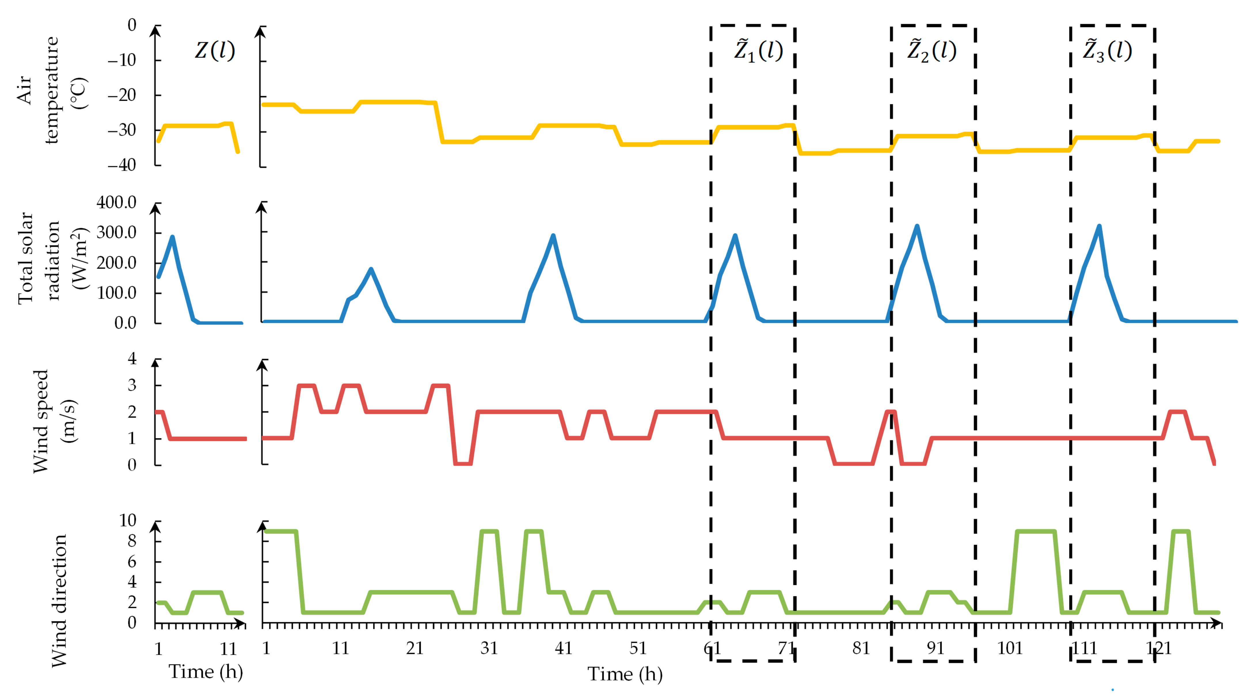
2.2. Technique and Tools for Air Temperature Prediction

In the general case, the problem of predicting the time series values is formulated as follows. Let the set $X=\left\{x_j^i\right\}$ be a multidimensional time series of retrospective data, where $i=\overline{1,n_s}$, $j=\overline{1,n_e}$, $n_s$ is a number of time series, and $n_e$ is a number of elements in time series. $X$ consists of $n_s$ time series that represent retrospective data about $n_s$ meteorological parameters. Thus, $x^i=\left\{x_1^i,x_2^i,\dots ,x_{n_e}^i\right\}$ is an ith one-dimensional time series corresponding to the ith meteorological parameter. It is required to predict the value $x_{n_e+1}^w$, where $w\in \overline{1,n_s}$ is a predicted meteorological parameter.

Based on achievements in the field of predicting time series, including forecasting air temperature, we conclude that the following methods are most in-demand in practice [32,33]: regression methods, autoregressive methods, neural network-based methods, and methods based on the support vector machine.

As a rule, regression and autoregressive methods are mainly used to predict the minimum, maximum, or average parameters of a time series, for example, air temperature [34]. These methods do not have sufficient accuracy in comparison with the other two groups of methods [35,36]. Therefore, in many cases, applying methods based on neural networks and support vector machines is preferable for modeling and predicting. An extensive bibliography is devoted to applying such methods (see, for example, [37,38]). The use of neural networks with various structures for predicting air temperature is considered in [39,40,41]. In [42], a comparison is made between support vector methods and neural networks. However, these methods also have some disadvantages [43,44]. In particular, methods based on neural networks and support vectors require lengthy training to apply the obtained model to new time series. Otherwise, the specific features of a series will misrepresent the prediction based on the previous training. In practice, this is not always convenient since it often requires HPC use.

In this regard, we propose a technique using the concept of similarity for time series fragments [45,46]. In [46], a similar technique is efficiently applied to predict the electricity demand. In addition, the prediction problem for several subject domains is successfully solved similarly in [45]. The authors also discuss the advantages of using this technique in comparison with the methods discussed above. Among these advantages is the accuracy in prediction.

In this paper, we focus on air temperature prediction. Within the proposed technique, the fragment $Z(n_e+1)=\left\{z_j^i\right\}$ of an hourly time series is given, where $z_j^i=x_j^i$, $i=\overline{1,n_s}$, $j=\overline{n_e-n_z+1,n_e}$, and $n_z$ is a number of elements in $Z$. This fragment precedes the $(n_e+1)\mathrm{th}$ time moment for a prediction. Then, a search for similar weather conditions ${\tilde{Z}}_1(n_e+1),{\tilde{Z}}_2(n_e+1),\dots ,{\tilde{Z}}_{n_q}(n_e+1)$ in the past with the same dimensions is carried out. Weather condition similarities are determined using the similarity function (SF) described below. Finally, the air temperature at the given time is predicted based on the found weather conditions applying the prediction function (PF).

Retrospective data on weather conditions in a specific location are used as input. A search for similar weather conditions in the past is characterized by low computational complexity. At the same time, the adjustment of a number of the PF parameters to minimize the prediction error requires HPC use.

We provide two iterative stages in applying the considered technique. The first stage is intended to adjust the PF parameters. Within the second stage, we use PF to predict the air temperature in locations for which the function parameters have been adjusted. When additional observation data accumulates, we extend the multidimensional time series $X$ and return to the first stage to re-adjust the PF parameters.

Stage 1. Obtain the multidimensional series $X$ of meteorological data for a specific location. The prediction period is taken from $n_{l+1}$ to $n_e$, i.e., we calculate the values of air temperature for ${\tilde{x}}^w=\left\{{\tilde{x}}_{n_{l+1}}^w,{\tilde{x}}_{n_{l+2}}^w,\dots ,{\tilde{x}}_{n_e}^w\right\}$, $w\in \overline{1,n_s}$. Next, determine the search set $\overline{X}=\left\{{\overline{x}}_1^i,{\overline{x}}_2^i,\dots ,{\overline{x}}_{n_l}^i\right\}$ and evaluation set $\overline{\overline{X}}=\left\{{\overline{\overline{x}}}_{n_l+1}^i,{\overline{\overline{x}}}_{n_l+2}^i,\dots ,{\overline{\overline{x}}}_{n_e}^i\right\}$, $i=\overline{1,n_s}$. $\overline{X}\subset X$ is a set used for searching the fragments ${\tilde{Z}}_1(l)$,${\tilde{Z}}_2(l)$,${\tilde{Z}}_3(l)$, etc. that are similar to $Z(l)$, ${\overline{x}}_j^i=x_j^i$, $j=\overline{1,n_l}$, $l\in \overline{n_l+1,n_e}$. The rest of the time series ${\overline{x}}^i$ are used to reduce the prediction error, $i\in \overline{1,n_s}$ and $i\ne w$. $\overline{\overline{X}}\subset X$ is used to evaluate the prediction error of the values ${\tilde{x}}_{n_{l+1}}^w,{\tilde{x}}_{n_{l+2}}^w,\dots ,{\tilde{x}}_{n_e}^w$ in comparison with the known values ${\overline{\overline{x}}}_{n_l+1}^w,{\overline{\overline{x}}}_{n_l+2}^w,\dots ,{\overline{\overline{x}}}_{n_e}^w$, ${\overline{\overline{x}}}_j^w=x_j^w$, $j=\overline{n_{l+1},n_e}$.

For each lth predicted element from ${\tilde{x}}^w$, searching the fragments ${\tilde{Z}}_1(l)$, ${\tilde{Z}}_2(l)$, ${\tilde{Z}}_3(l)$, etc. using SF is implemented in the following way: forming ${\tilde{Z}}_v(l)$ and calculating $b=SF\left(P,Z(l),{\tilde{Z}}_v(l),l\right)$, where $b$ is a Boolean variable that indicates whether the fragment ${\tilde{Z}}_v(l)$ is similar ($b=1$) or not ($b=0$) to $Z$, $P=\left\{p_i\in D_i\right\}$ is a set of adjusted parameters, $D_i$ is a domain of $p_i$, $l\in \overline{n_l+1,n_e}$, $i=\overline{1,n_p}$, $v=\overline{1,n_f}$, $n_f$ is a number the compared fragments in $\overline{X}$. Figure 3 illustrates searching ${\tilde{Z}}_1(l)$, ${\tilde{Z}}_2(l)$, ${\tilde{Z}}_3(l)$, etc.

The fragment of four-dimensional time series used as retrospective data in experiments is demonstrated in

Table 1. Fragment of multidimensional time series.

Air Temperature (°C)	Wind Speed (m/s)	Wind Direction	Total Solar Radiation (W/m2)
−24.2	0	Calm	74.1
−23.7	0	Calm	87.8
−22.5	0	Calm	128.6
−21.5	1	North-West	176.3
−21.5	1	North-West	116.2
−21.7	2	North-West	53.3
−21.9	2	North-West	4.7
−22.2	2	North-West	0

. Wind directions are “Calm”, “North”, “North-West”, “North-East”, “South”, “South-West”, “South-East”, “West”, and “East”. Upon request, the data are available from the external WPS service registered on the GIS portal. This WPS service performs preliminary data processing extracted from the open data source https://rp5.ru/Weather_in_the_world (accessed on 29 October 2021) for a given period.

SF is based on determining the correlation between the compared fragments. Algorithm 1 shows the pseudocode for an algorithm of the SF operation.

Algorithm 1. Algorithm of the SF operation.

1 function $SF\left(P,Z(l),\tilde{Z}(l),l\right)$   2   if $\exists i=\overline{1,n_s}\left|{\tilde{z}}_{n_z}^i(l)-z_{n_z}^i(l)\right.\left|>p_i\right.$ then   3      return 0;   4   end if   5   if    $\forall i=\overline{1,n_s}\frac{{\displaystyle {\sum }_{j=n_z-p_{i+n_s}+1}^{n_z}\left({\tilde{z}}_j^i(l)-\frac{1}{p_{i+n_s}}{\displaystyle {\sum }_{l=1}^{p_{i+n_s}}{\tilde{z}}_j^i(l)}\right)\cdot \left(z_j^i(l)-\frac{1}{p_{i+n_s}}{\displaystyle {\sum }_{l=1}^{p_{i+n_s}}{z}_j^i(l)}\right)}}{\sqrt{{\displaystyle {\sum }_{j=n_z-p_{i+n_s}+1}^{n_z}{\left({\tilde{z}}_j^i(l)-\frac{1}{p_{i+n_s}}{\displaystyle {\sum }_{l=1}^{p_{i+n_s}}{\tilde{z}}_j^i(l)}\right)}^2\cdot {\left(z_j^i(l)-\frac{1}{p_{i+n_s}}{\displaystyle {\sum }_{l=1}^{p_{i+n_s}}{z}_j^i(l)}\right)}^2}}}>p_{i+2n_s}$    then   6     return 1;  7   else   8     return 0;  9   end if   10 end function

Values of parameters from $P$ are adjusted to minimize the prediction error. The adjusted parameters determine the permissible length of time series and correlation coefficient, as well as limits on modules of the difference for the air temperature, total solar radiation, wind speed, and wind direction. To adjust these parameters, we generate a set of combinations of the parameter values randomly selected from the parameter domains. Then we predict ${\tilde{x}}^w$ using PF. Algorithm 2 shows the pseudocode for an algorithm of the PF operation, where $l\in \overline{n_l+1,n_e}$.

Algorithm 2. Algorithm of the PF operation.

1 function $PF(X,Z(l),P,l,n_l)$  2   $sum=0,\hspace{0.33em}count=0$;  3   for $k$ from $((l-1)\mathrm{mod}{n}_z)+n_z$ to $n_l$ increment $k=k+n_z$  4     if ($k<l-n_z-1$ or $k>l+n_z-1$) then  5       $\tilde{Z}(l)=\left\{{\overline{x}}_j^i\right\}$, $i=\overline{1,n_s}$, $j=\overline{k-n_z+1,k}$;  6       if ($SF(P,Z(l),\tilde{Z}(l),l$) then  7         $sum=sum+{\overline{x}}_{k+1}^w-{\overline{x}}_k^w$;  8         $count=count+1$;  9       end if  10     end if  11   next $k$;  12   if ($count<3$) then  13     ${\tilde{x}}_l^w=z_{n_z}^w(l)$;  14   else  15     ${\tilde{x}}_l^w=z_{n_z}^w(l)+\frac{sum}{count}$;  16   end if  17   return ${\tilde{x}}_l^w$;  18 end function

We select mean absolute error (MAE) for measuring the prediction errors. In our case, MAE is defined as follows:

$$MAE=\frac{1}{n_e-n_l}{\displaystyle {\sum }_{l=n_l+1}^{n_e}\left|{\overline{\overline{x}}}_l^w-\mathrm{PF}(X,Z(l),P,l,n_l)\left|\to min\right.\right.}.$$

Stage 2. When the parameters from $P$ were adjusted, we can use PF with the optimal values of these parameters in different applications in which it is required to model the hourly air temperature. To accomplish this, we determine the lth predicted element of a time series and the fragments $Z(l)$ that precedes this element in the loop for $l$ and call PF. In modeling, we can extend $X$ by both the real and modeled data. Periodically, we can return to the first phase and re-adjust the parameters when the extended data exceeds a specific size.

Within the proposed approach, we develop an application for adjusting the PF parameters. It is applied to solve the pattern recognition problem to determine similar weather conditions in the past and predict air temperature in the future based on them. We adjust the PF parameters by the multi-start method [47] used jointly with the Nelder–Mead method [48] applied to searching local extremums.

The multi-start method is based on the search for local optima of a function. It can use various algorithms of the descent from the set $S$ that consists of $m$ starting points to the local optima $u_1,u_2,\dots ,u_m$. When local optima have been found, the value $u^{*}=\underset{i=\overline{1,n_{sp}}}{min(max)u_i}$ is selected as a global optimum of the studied function.

In general, the workflow structure for the multi-start method implementation includes the following four main stages:

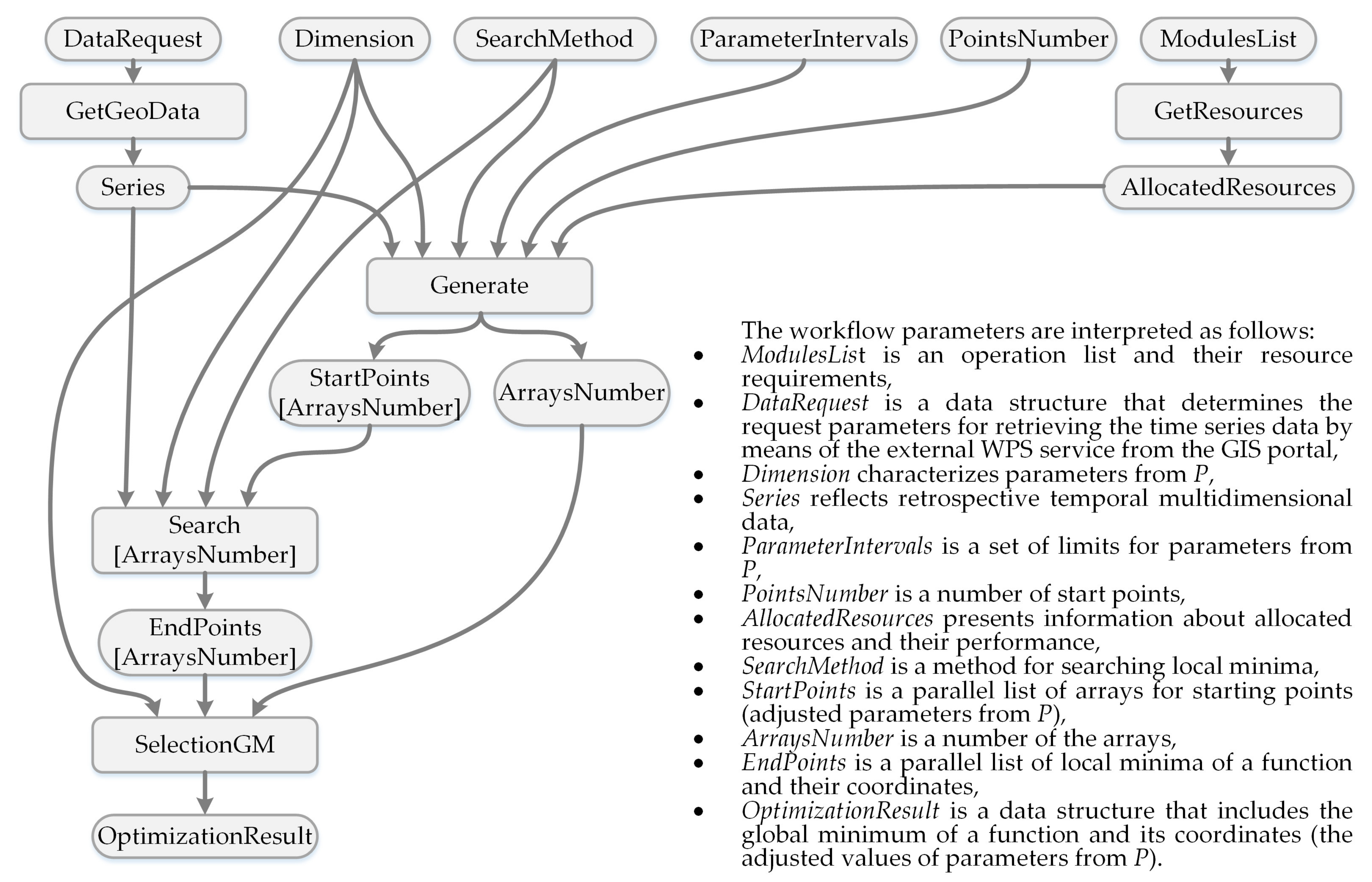
• generating the set $S$ of starting points,
• distributing starting points among resources of the computing environment,
• parallel descending from the starting points to the local optima $u_1,u_2,\dots ,u_{n_{sp}}$ using the Nelder–Mead method,
• selection of the global optimum $u^{*}$ from $u_1,u_2,\dots ,u_{n_{sp}}$.

An optimization of a multiextremal function using the multi-start method is performed on heterogeneous resources with different computational characteristics. The distribution starting points on resources is a non-trivial problem. We need to solve the following problem:

$$t_{ms}=\left[\underset{i=\overline{1,n_c}}{max}\left(q(\mathrm{PF}\right)\frac{n_i}{r_i}+v_i(n_i)\right]\to min,$$

$${\displaystyle \sum _{i=1}^{n_c}{n}_i=n_{sp},}$$

where $n_c\ge 1$ is a number of cores, $n_{sp}>1$ is a number of start points, $q(\mathrm{PF})>0$ is an average number of elementary operations that is required to find a local minimum of SF from one starting point, $n_i\ge 0$ is a number of starting points that will be processed on the ith core, $r_i>0$ is a number of elementary operations that are processed by the ith core per time unit, $v_i\ge 0$ is overheads of the ith core that depend on the number of processed starting points, and $t_{ms}>0$ is an evaluation of a workflow makespan.

This problem is NP-hard [49]. An increase in the number of starting points per core reduces core use overheads. In this regard, we implement a new strategy of the multi-start method execution, taking into account execution time evaluations for application modules and resource performances. We use the evaluations of the module execution time in different nodes of the computing environment that are obtained based on testing the module in these nodes. Such testing is implemented in the continuous integration of application modules. We include system modules from the API of an agent-based meta-monitoring system [50] into the workflow. These system modules provide the search and capture of environment resources, prediction of their performances in executing the application modules, taking into account obtained evaluations and distribution of the computational load between the captured resources. The advantages of the new strategy are effectively balancing the computational load of resources and decreasing the workflow makespan.

Figure 4 illustrates the workflow for solving the problem of adjusting the PF parameters. Parameters and modules of the workflow are drawn with circles and ovals, respectively. The arrows show transferring parameters between modules.

The workflow includes four modules. GetResources is a system module. It receives a workflow module list with limits on the number of launches of their instances in the computing process. Then it captures resources, evaluates their performance with respect to workflow module executions using agents of the meta-monitoring system, and allocates these resources for module executions. GetResources transfers the information about allocated resources and their performance to the module Generate. Thus, we implement an additional stage of the problem-solving scheme in comparison with the classical multi-start method and provide the data decomposition based on the heuristic information about the performance of resources. The module GetGeoData represents a call of the external WPS service for retrieving the retrospective time series data from the GIS portal.

The module Generate generates a set of start points for each job executed on allocated resources. The number of processed start-points for each job corresponds to the performance of resources allocated to execute the job. Such mapping promotes the efficient use of allocated resources. A set of start-points is generated by varying random point coordinates (values of parameters from $P$).

The module Search implements an algorithm for the descent from the start point to a local minimum using the Nelder–Mead method. Elements of the parallel lists StartPoints and EndPoints are the input and output variables of this module. They are processed independently of each other by the Search instances. Each instance is a message passing interface (MPI) program. Within the module Search execution, the OT interpreter runs its instances on the allocated resources. Finally, the module SelectionGM combines the obtained local minima and returns a minimum value among them as the global minimum of the function.

Thus, we provide the program library that includes PF for hourly air temperature prediction and workflow-based WPS service for adjusting the PF parameters for a specific territory. End-users can also use PF from the library with the default parameters. The default parameter values are adjusted for locations in the Baikal natural territory.

3. Results and Discussion

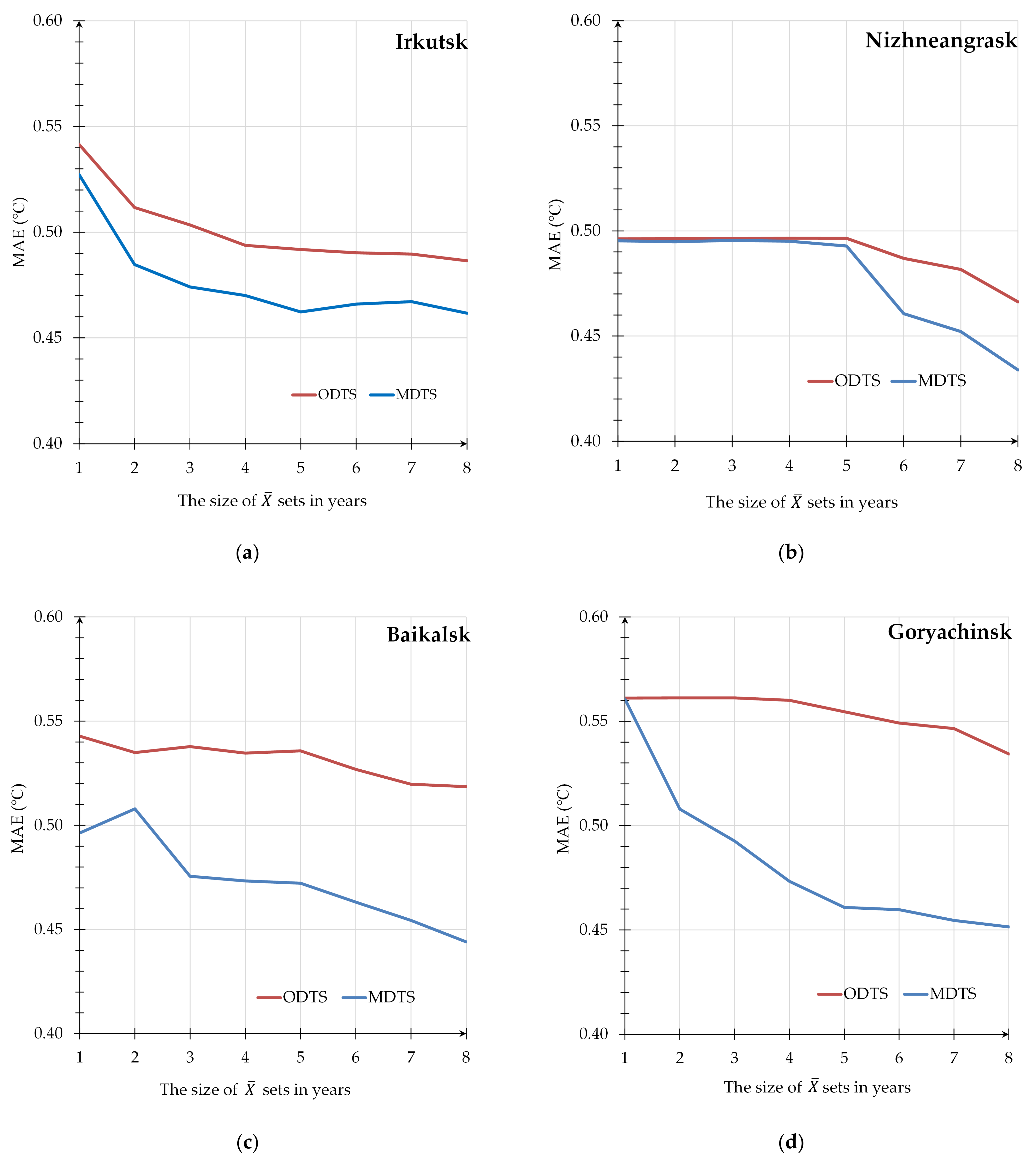
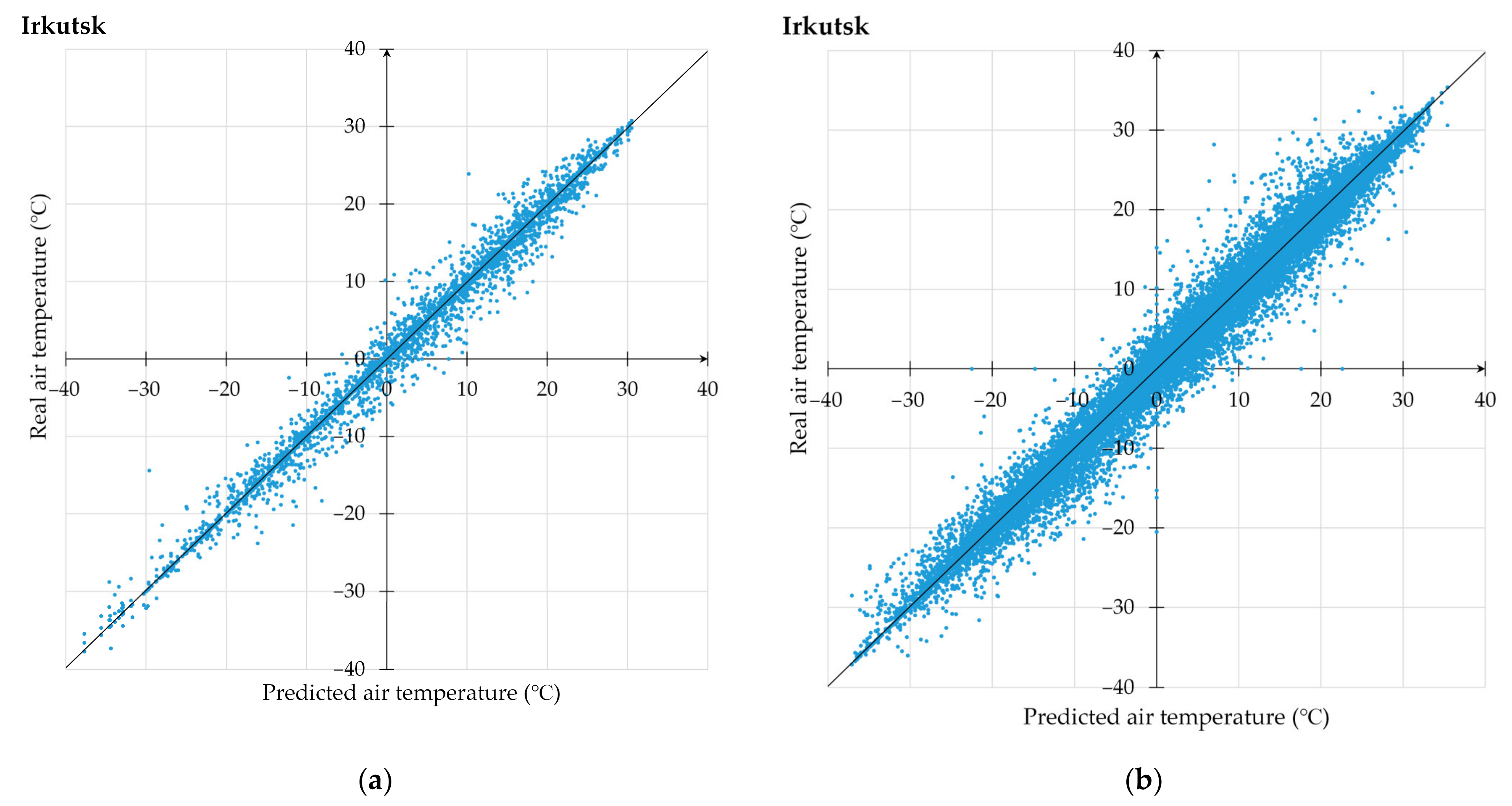
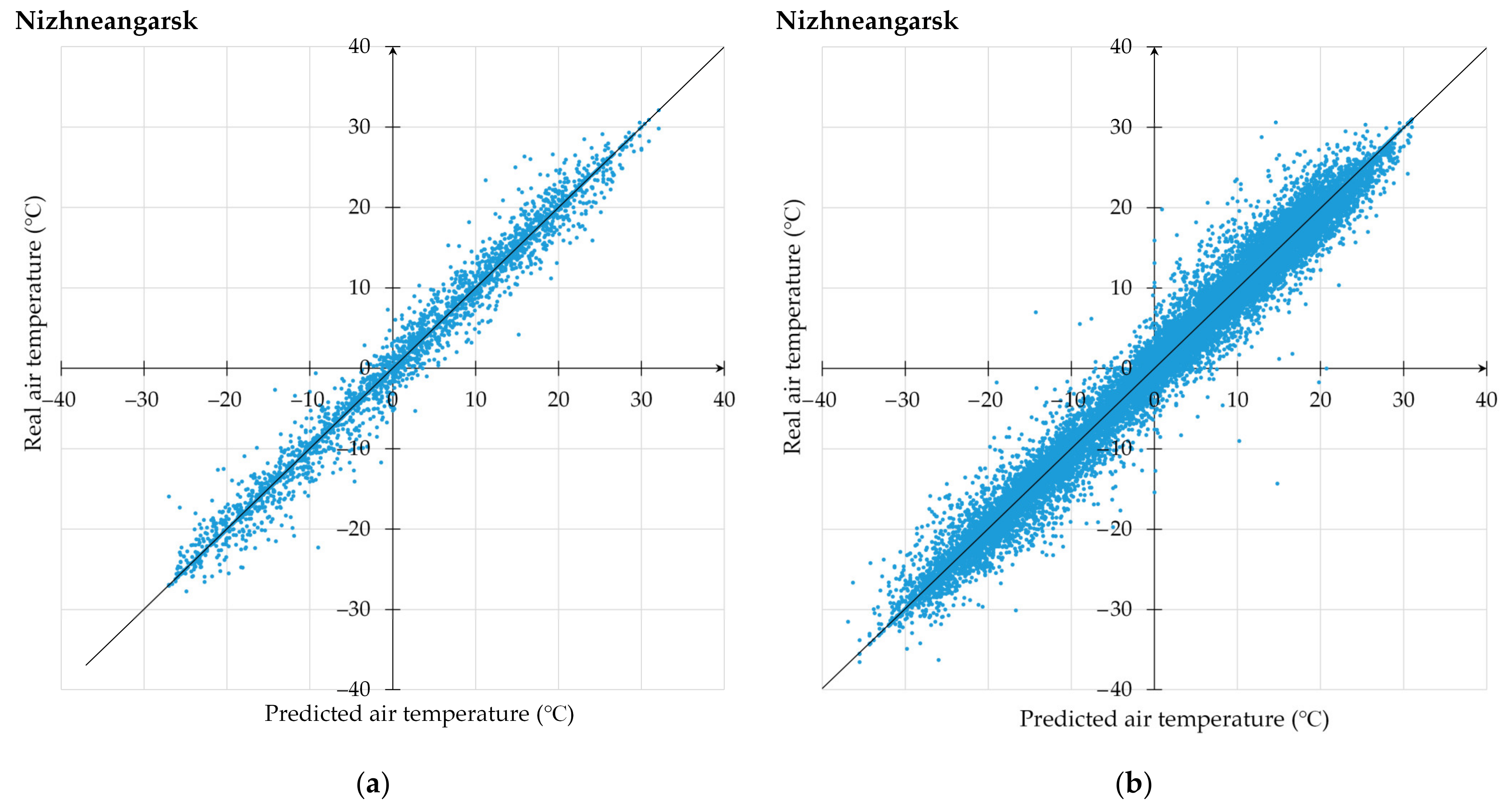
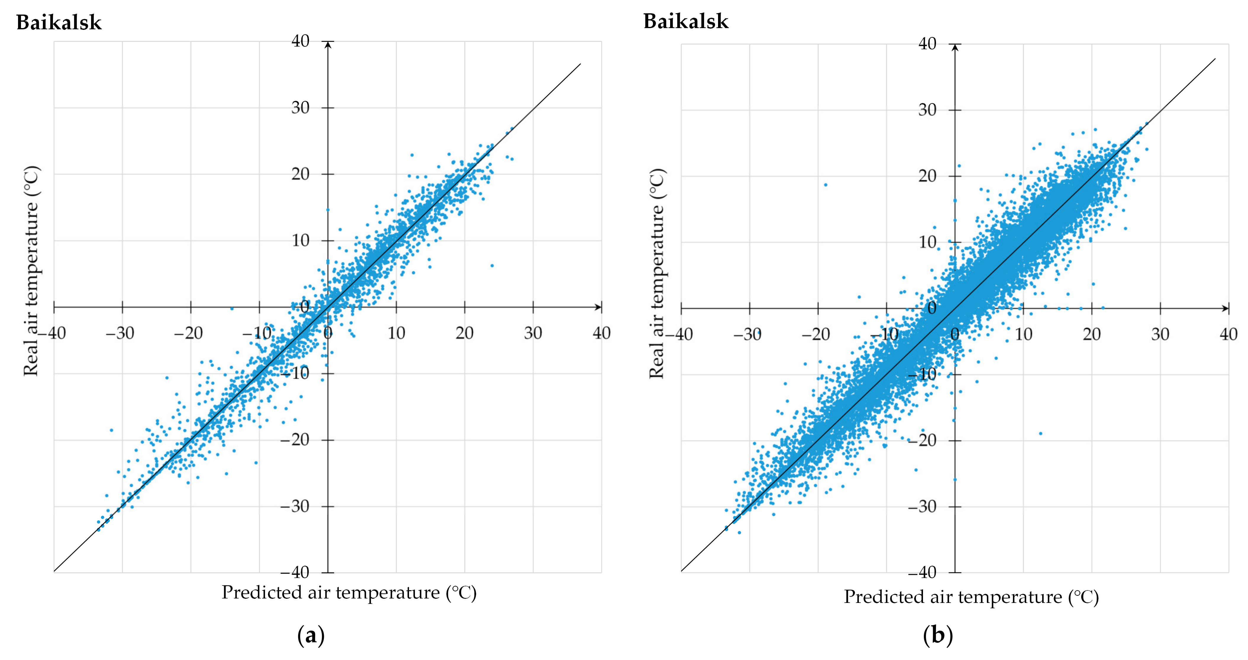
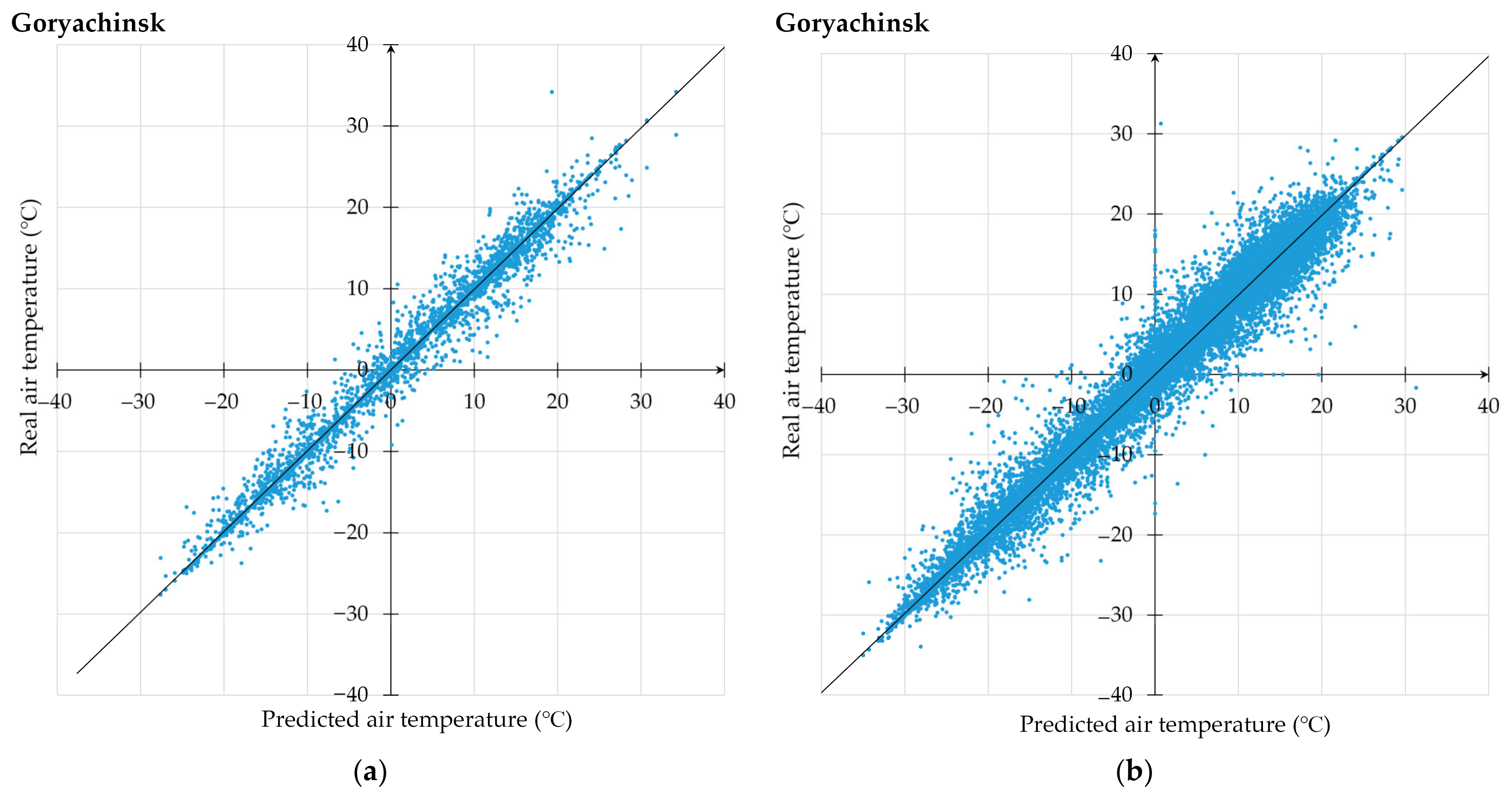
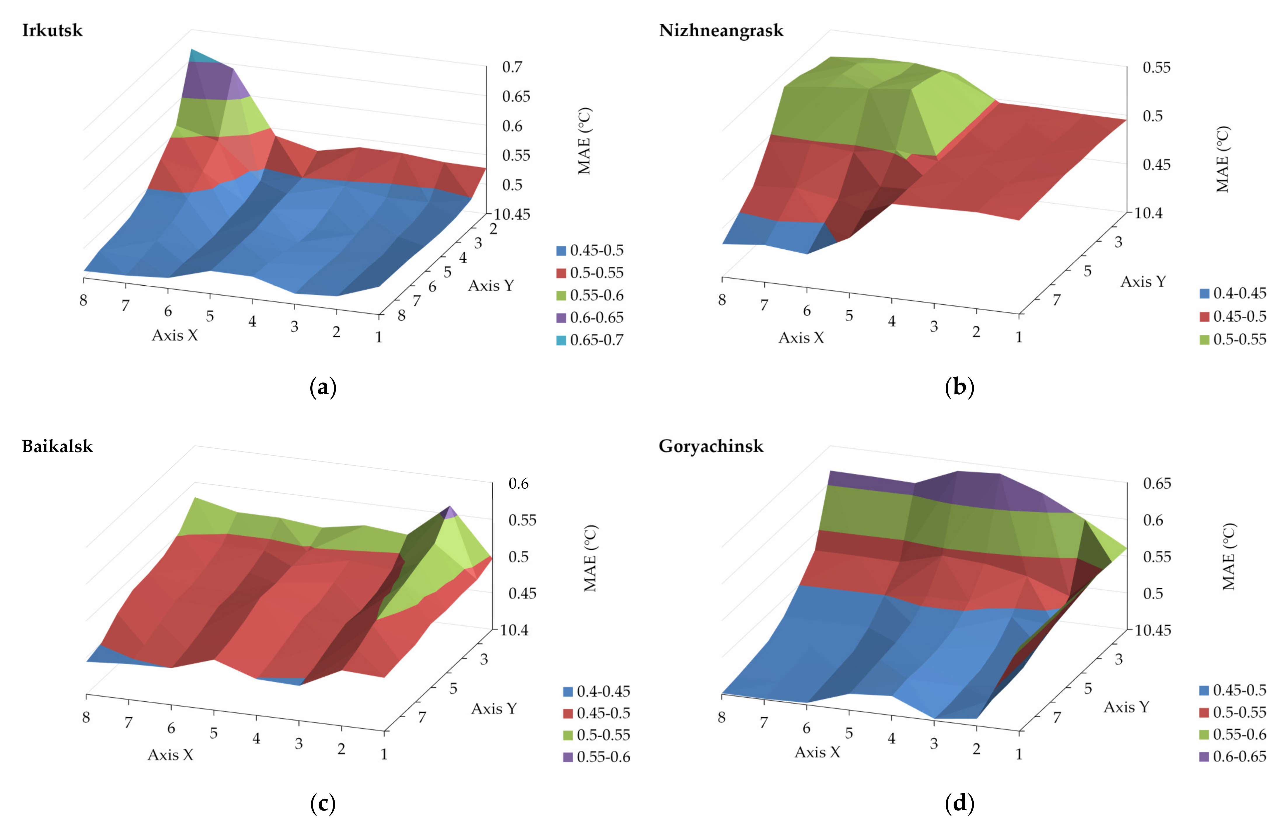
3.1. Proposed Technique Use for Air Temperature Prediction

We analyzed the impact of using additional data to predict air temperature in the proposed technique. To this end, we predicted air temperature for the given period. The prediction was carried out for four locations (i.e., Irkutsk, Nizhneangarsk, Baikalsk, and Goryachinsk) with different weather conditions. We used retrospective multidimensional time series obtained applying the WPS service registered on the GIS portal to extract and process meteorological data from [51]. This time series represents data from 1 January 2011 to 31 December 2019, collected by weather stations at the selected locations.

Within the experiment, we changed the sizes of $\overline{X}$ for Stage 1 and Stage 2 of the proposed technique in equal proportion. For comparison, we predicted in two ways. In the first case, we made a prediction based on one-dimensional time series (ODTS) of air temperature. In the second case, we predicted based on multi-dimensional time series (MDTS) that includes data about air temperature and total solar radiation, as well as wind speed and direction.

The prediction error estimated using the MAE is shown in Figure 5. We can see that in our experiment, additional data allowed the MAE to be reduced in all four cases. This is especially evident for the predictions in Baikalsk (Figure 5c) and Goryachinsk (Figure 5d). In the cases of Irkutsk (Figure 5a) and Nizhneangarsk (Figure 5b), the MAE decrease was smaller, since air temperature changes are more stable there. Thus, the impact of additional meteorological data varies in degree, which is usually due to the microclimate features of a specific location. Nevertheless, using additional data has a positive effect on the accuracy of the air temperature prediction.

In the next experiment, we used the same data. We divided the set $X$ related to Irkutsk to the $\overline{X}$ and $\overline{\overline{X}}$ sub-sets, which time series included $n_l=\mathrm{70,080}$ and $n_e-n_l=8760$ elements, respectively. We adjusted the PF parameters using $\overline{X}$ and predicted ${\tilde{x}}_{n_l+1}^w,{\tilde{x}}_{n_l+2}^w,\dots ,{\tilde{x}}_{n_e}^w$ and ${\tilde{x}}_n^{w}ma{x}_{+1},{\tilde{x}}_n^{w}ma{x}_{+2},\cdots ,{\tilde{x}}_{n_l}^w$. In the first case, we evaluated prediction error using $\overline{\overline{X}}$. In the second case, we applied $\overline{X}$.

Figure 6a,b demonstrate the prediction error scatter for the first and second cases, respectively. In both figures, the prediction error scatters are similar. This is confirmed by MAE calculated for both predictions with the same PF parameters (

Table 2. Experimental statistics.

Strategy	Number of Launches	Average Execution Time (s)	Total Execution Time (s)	Average Overheads (s)
1	10	2923.62	3819.97	33.55
2	100	323.17	3223.97	295.51
3	10	2902.05	2962.34	34.32

). Based on these results, we conclude that the PF with adjusted parameters allows prediction of air temperature with sufficient accuracy. In terms of prediction accuracy, we believe that our results are comparable with the results obtained based on neural networks and other prediction methods [39].

Similar calculations were performed for Nizhneangarsk (Figure 7), Baikalsk (Figure 8), and Goryachinsk (Figure 9). Generally, their results confirm our conclusions with respect to Irkutsk.

Figure 10a shows the dependence of MAE on the size of $\overline{X}$ used at the first (x-axis) and second (y-axis) stages of the proposed technique for predicting the air temperature with respect to Irkutsk. The number of elements in $\overline{X}$ varied from 8760 to 70,080 for both stages. This corresponds to data sizes from 1 to 8 years. The figure shows that a simultaneous increase in the number of elements in $\overline{X}$ along the x-axis and y-axis often provides a decrease in MAE. In addition, increasing the number of elements in $\overline{X}$ along the y-axis also contributes to reducing MAE. Thus, it can be assumed that expanding $\overline{X}$ with current observations will provide a decrease in MAE when predicting air temperature using the same pre-adjusted PF parameters.

The results of predicting the air temperature with a similar change in the number of elements of $\overline{X}$ for Nizhneangarsk, Baikalsk, and Goryachinsk are shown in Figure 10b–d correspondingly. Generally, they confirm our conclusions about the $\overline{X}$ size changes considered for Irkutsk.

The developed software library and workflow-based WPS service have been used for modifying the service of simulation modeling environmentally friendly equipment considered in [52]. This service was applied to evaluate ${\mathrm{CO}}_2$ reduction because of partially using heat pumps instead of the coal-fired boiler within heating systems of infrastructure objects in the Baikal natural territory.

We replaced the hourly air temperature prediction function used in the service with PF, the parameters of which were adjusted considering the weather conditions of the location for the simulated infrastructure objects. The use of PF allowed us to specify the heating season characteristics and clarify the reduction in ${\mathrm{CO}}_2$ emissions.

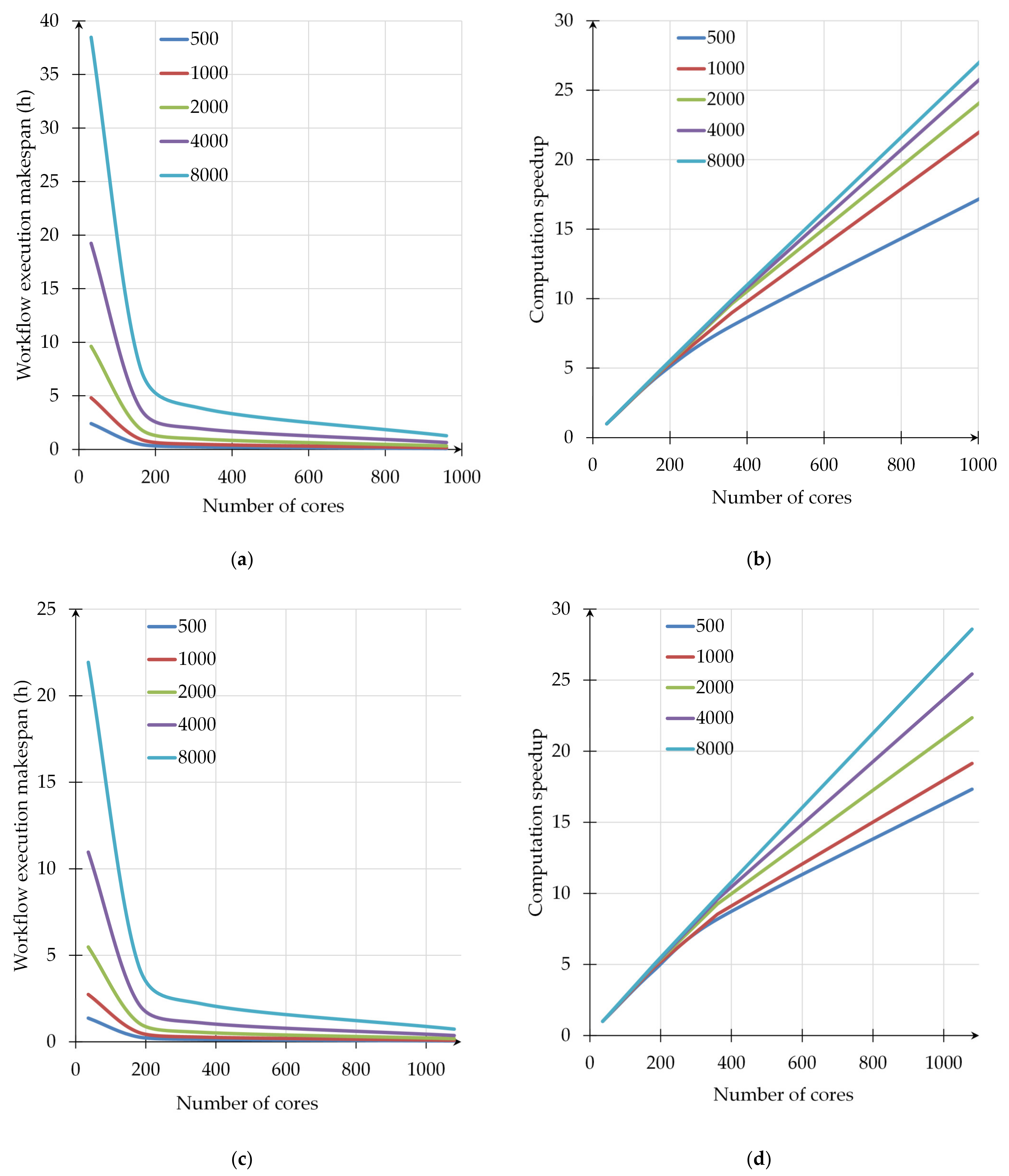
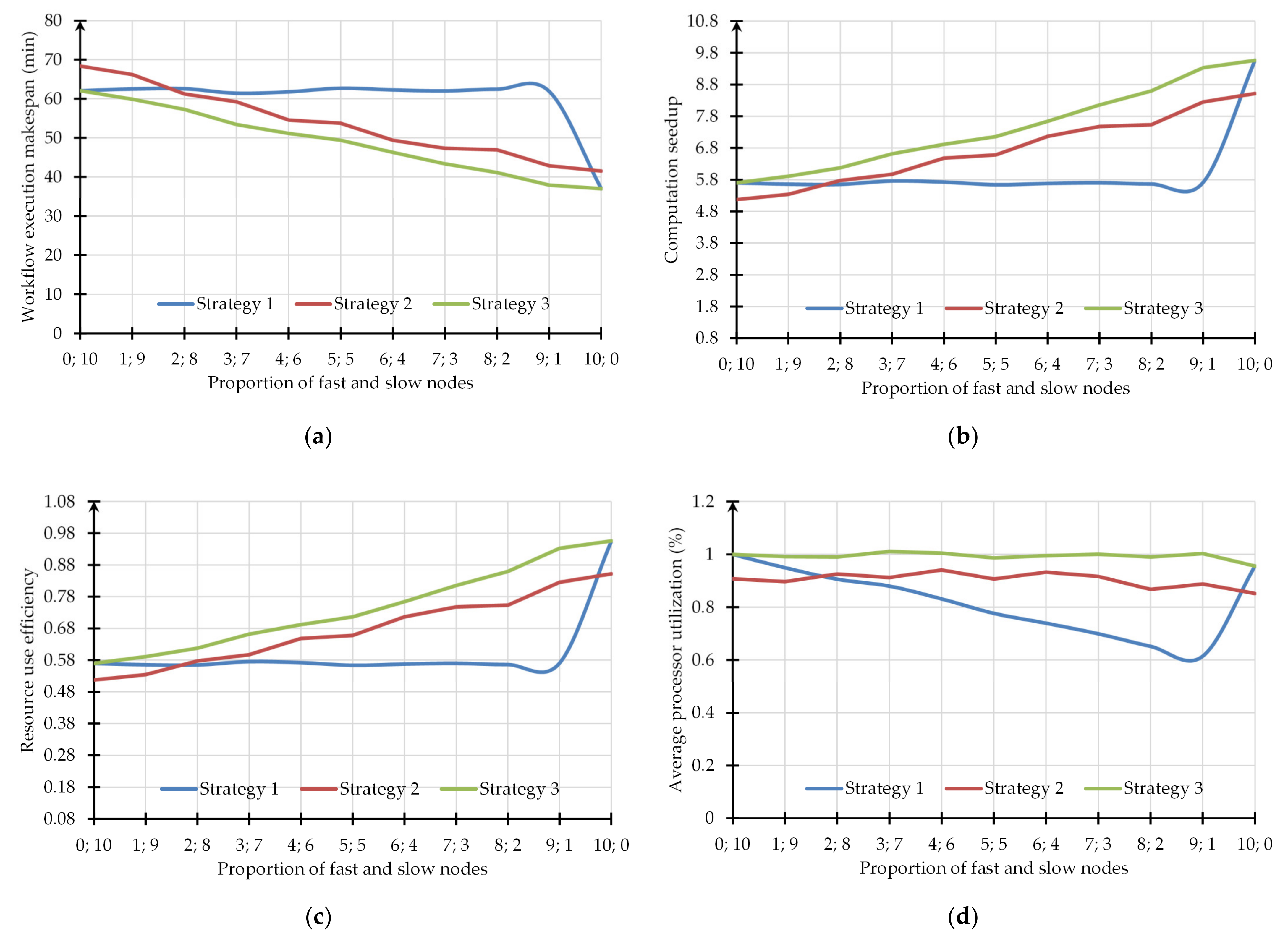
3.2. Comprehensive Analysis of Computational Experiments

The workflow-based application is launched when the WPS service is called to adjust the PF parameters. We solved the problem of adjusting the PF parameters to the Irkutsk weather condition on two HPC clusters of the public access Irkutsk Supercomputer Center [53] in turn. Cluster nodes had the following characteristics: 2 processors Intel Xeon CPU X5670 (18 core, 2.1 GHz, 128 GB of RAM) for a node of the first cluster; 2 processors AMD Opteron 6276 (16 core, 2.3 GHz, 64 GB of RAM) for a node of the second cluster. The maximum number of cores used was varied from 32 to 1024 for the first cluster (from 36 to 1080 for the second cluster).

Figure 11a,b demonstrate workflow execution makespan (a) and computation speedup (b) in adjusting the PF parameters obtained on the first cluster using 500, 1000, 2000, 4000, and 8000 start-points. Figure 11c,d show the makespan (c) and speedup (d) obtained on the second cluster. In both cases, we observed a significant reduction in the workflow execution makespan with a growth in the number of cores used. Reducing the makespan was achieved by increasing the computation speedup due to the growth in the number of cores used.

The heterogeneity of node characteristics when distributing the computational load is a cause of a non-trivial problem. The need to evaluate the workflow execution makespan on different nodes of the computing environment complicates solving this problem. In this regard, it is essential to have strategies for distributing the computational load that enable us at least partially to solve the problem.

We compared the following three strategies for distributing the computational load between nodes:

• Launching an equal number of jobs on each node by a user.
• Loading free nodes from the common job queue. This strategy is used in practice by well-known meta-schedulers such as GridWay and Condor DAGMan, as well as LRMs for homogenous resources, for example, LSF [54].
• Launching the number of jobs on each node in proportion to the node’s performance, taking into account the evaluated job execution time on this node. We implemented and applied this strategy in OT using the meta-monitoring system to predict job execution time on nodes represented by agents that took into account the results of the application module testing in these nodes.

Executing the module search determines the main contribution to the workflow execution makespan. Therefore, we launched jobs for executing this module in an environment consisting of 10 fast and slow nodes presented in different proportions. Nodes had the following characteristics: 2 processors Intel Xeon CPU X5670 (18 core, 2.1 GHz, 128 GB of RAM) for a fast node; 2 processors AMD Opteron 6276 (16 core, 2.3 GHz, 64 GB of RAM) for a slow node. Nodes were also part of two HPC clusters of the Irkutsk Supercomputer Center. Thus, we used from 320 to 360 cores in each experiment.

We used three strategies for distributing the computational load between nodes for each launch within these experiments. We evaluated job execution time on fast and slow nodes for the third strategy by testing the module on both types of nodes. Experimental statistics are presented in Table 2. For each strategy in Table 2, we give the number of module instance launches, average execution time for an instance, total execution time for all instances, and average overheads. The overheads are related to queuing, starting, and controlling module instances and data transferring. The statistics were obtained by searching the global minimum of PF using 2000 start points on five fast and five slow nodes.

Module instance in the second strategy had a lower computational load (processing fewer start-points). Therefore, the average execution time for an instance in the second strategy was less than for the other strategies. Due to capturing resources, the third strategy was slightly inferior to the first strategy in average overheads. However, it out-performed the second strategy in the average execution time for an instance. Moreover, the third strategy was superior to others in the total execution time for all instances. This advantage of the first strategy was achieved because of the computational load’s better distribution, taking into account the module execution time in the allocated nodes.

Figure 12a shows the workflow execution makespan based on the three strategies of distributing the computational load for different proportions of fast and slow nodes. The module Search contributed most to the workflow execution makespan. Applying the third strategy produced a steady reduction in the workflow execution makespan with the growth of fast nodes. However, the third strategy outperformed the second strategy in the reduction for all proportions of nodes. At the same time, the first strategy was inferior to the third strategy in most of the proportions of nodes. It produced a workflow execution makespan equal to the same makespan obtained within the third strategy in the environment consisting of homogeneous resources only.

Within the first strategy, the instances of the module Search processed the same number of starting points, i.e., they had approximately the same computational load. When using nine fast nodes, jobs started on these nodes for the module Search were rapidly executed. At the same time, we had to wait a long time to complete a job for the same module on a slow node. All such jobs were executed at about the same speed for ten fast nodes. In this case, a significant reduction in the workflow execution makespan was achieved compared to the proportion of the fast and slow nodes, equivalent to 9 to 1.

Changes in computation speedup following the increase of fast nodes are demonstrated in Figure 12b. Here, computation speedup is calculated as the ratio of the workflow execution at one fast node to the workflow execution makespan in an environment consisting of ten fast and slow nodes, presented in different proportions. The third strategy demonstrated improvement in computation speedup for all proportions of fast and slow nodes in comparison with the second strategy. It also outperformed the first strategy in computation speedup for most proportions, except in two cases when we used completely homogeneous nodes.

The resource use efficiency shown in Figure 12c is defined as the ratio of computation speedup to the number of nodes used. As for the third strategy, we can see that the efficiency was close, changing from 0.57 to 0.97. The first and second strategies were inferior to the third one on this objective, as was the computation speedup.

Finally, Figure 12d represents the average CPU utilization for the resources used. In most combinations of fast and slow nodes, the first strategy provided a better average CPU utilization than the other strategies.

Based on the analysis of the experimental data, we draw the following conclusions on the computing environment considered:

• Using at least one slow node negatively affects workflow execution makespan, computation speedup, and resource use efficiency when applying the first strategy. At the same time, values of the average CPU utilization close to 1 were achieved when using the computing environment entirely consisting of homogeneous nodes.
• Within the second strategy, more instances of the module Search were generated. All instances involved queueing before a launch. In addition, it was necessary to transfer data and check the execution status for each instance. Therefore, the second strategy was characterized by more overheads. These overheads were the main contributors to an increase in the workflow execution makespan in comparison with the other strategies.
• The advantages of the third strategy were achieved due to distributing the computational load on resources according to their performance. The demonstrated computation speedup with an increase in the number of used fast nodes and efficiency of their use close to 1 determined the good scalability of distributed computing.

Ensuring the scalability of distributed computing is a significant problem because the used distributed computing environments systems can include resources with different computational characteristics and capabilities.

The results of the experimental analysis carried out in the computing environment demonstrate the advantages of the proposed strategy of computational load distribution in OT in comparison with other strategies often applied in practice.

The advantages are in the improvement of both the users’ objectives for the problem-solving quality (i.e., growing computation speed and reducing workflow execution makespan) and preferences of resource providers in increasing the resource use efficiency and average utilization of their processors. This is primarily due to the potential for OT to include system modules into the workflow for searching and capturing resources, predicting their performance, and distributing the computational load between these resources by agents. Moreover, the more significant the computing environment heterogeneity, the more visible the advantages of the proposed strategy in comparison with others considered.

4. Conclusions

In this paper, we proposed an approach to integrating WPS services with workflow-based scientific applications within the GIS portal that supports solving environmental monitoring problems. Following this approach, users develop a scientific application based on modular programming and continuous integration, as well as organize a heterogeneous computing environment using the OT framework. Next, they form the workflows, automatically create WPS services, and register them on the GIS portal.

Applying the open WPS standard combined with a workflow technique provides the compositions of web services developed by different researchers and expands access to spatiotemporal data for GIS portal end-users.

From the perspective of HPC organization, we hope that the proposed approach ensures the availability and utility of resources of the heterogeneous distributed computing environment and computation scalability for other researchers. We want to provide interested professionals with improved possibilities for processing and exchanging data. In addition, we support the consistency of objectives for resource providers and their users due to implementing the continuous integration of the applied software using multi-agent technology.

The study results will promote carrying out data-intensive scientific experiments within the framework of environmental monitoring and provide interested organizations with access to the outcomes of these experiments. In turn, effective processing and analyzing spatiotemporal data will contribute to legislation preserving the Baikal natural territory and its ecological improvement by the Regional Government and Ministry of Natural Resources and Environment of the Russian Federation.

For many scientific and applied problems, reducing the processing time for spatiotemporal data is often a relevant issue. In this regard, we highlight the following directions for our future research:

• supporting the technology in-memory data grid (IMDG) [55] for applications developed in OT to provide processing spatiotemporal data in the RAM of nodes of the heterogeneous distributed computing environment,
• modifying the meta-monitoring system with respect to automating the identification and partial troubleshooting of faults in operating the system software and hardware to improve the reliability of spatiotemporal data processing based on IMDG.
• developing an additional converter to ensure compatibility with common workflow language (CWL) [56] to prevent re-development of the same workflows and thereby reduce the time of experiments.

References

- Makhonko, N.I.; Belousov, S.A.; Tarasova, E.A.; Plotnikova, Y.A. Information and communication technologies in environmental monitoring of climate change. IOP Conf. Ser. Earth Environ. Sci. 2021, 808, 012045. [Google Scholar] [CrossRef]
- Bychkov, I.V.; Ruzhnikov, G.M.; Hmelnov, A.E.; Fedorov, R.K.; Madzhara, T.I.; Popova, A.K. Digital Monitoring of Lake Baikal and its Coastal Area. In Proceedings of the 2nd Scientific-Practical Workshop Information Technologies: Algorithms, Models, Systems (ITAMS 2019), Irkutsk, Russia, 20 September 2019; CEUR-WS Proc.: Aachen, Germany, 2019; Volume 2463, pp. 13–23. Available online: http://ceur-ws.org/Vol-2463/paper2.pdf (accessed on 29 October 2021).
- Lega, M.; Casazza, M.; Teta, R.; Zappa, C.J. Environmental impact assessment: A multi-level, multi-parametric framework for coastal waters. Int. J. Sust. Dev. Plan. 2018, 13, 1041–1049. [Google Scholar] [CrossRef]
- Paul, P.; Aithal, P.S.; Bhuimali, A.; Kalishankar, T.; Saavedra, M.R.; Aremu, P.S.B. Geo Information Systems and Remote Sensing: Applications in Environmental Systems and Management. Int. J. Manag. Tech. Soc. Sci. 2020, 5, 11–18. [Google Scholar] [CrossRef]
- Fang, S.; Da Xu, L.; Zhu, Y.; Ahati, J.; Pei, H.; Yan, J.; Liu, Z. An integrated system for regional environmental monitoring and management based on internet of things. IEEE Trans. Ind. Inform. 2014, 10, 1596–1605. [Google Scholar] [CrossRef]
- Kussul, N.; Shelestov, A.; Skakun, S. Grid and sensor web technologies for environmental monitoring. Earth Sci. Inform. 2009, 2, 37–51. [Google Scholar] [CrossRef] [Green Version]
- Breunig, M.; Bradley, P.E.; Jahn, M.; Kuper, P.; Mazroob, N.; Rösch, N.; Al-Doori, M.; Stefanakis, E.; Jadidi, M. Geospatial data management research: Progress and future directions. ISPRS Int. Geo-Inf. 2020, 9, 95. [Google Scholar] [CrossRef] [Green Version]
- Lee, C.A.; Gasster, S.D.; Plaza, A.; Chang, C.I.; Huang, B. Recent developments in high performance computing for remote sensing: A review. IEEE J. Sel. Top. Appl. 2011, 4, 508–527. [Google Scholar] [CrossRef]
- Drăgan, I.; Fortiş, T.F.; Iuhasz, G.; Neagul, M.; Petcu, D. Applying self-* principles in heterogeneous cloud environments. In Cloud Computing; Antonopoulos, N., Gillam, L., Eds.; Springer: Cham, Switzerland, 2017; ISBN 978-3-319-85443-4. [Google Scholar]
- Huang, F.; Yang, H.; Tao, J.; Zhu, Q. Universal workflow-based high performance geo-computation service chain platform. Big Earth Data 2020, 4, 409–434. [Google Scholar] [CrossRef]
- The OGF Open Cloud Computing Interface. Available online: http://www.occi-wg.org/doku.php (accessed on 29 October 2021).
- The DMTF Open Virtualization Format. Available online: http://www.dmtf.org/standards/published_documents/DSP0243_1.0.0.pdf (accessed on 29 October 2021).
- The Open Source Geospatial Foundation. Available online: https://www.osgeo.org/ (accessed on 29 October 2021).
- Castronova, A.M. Models as web services using the open geospatial consortium (ogc) web processing service (wps) standard. Environ. Modell. Softw. 2013, 41, 72–83. [Google Scholar] [CrossRef]
- Foerster, T.; Schaeffer, B.; Brauner, J.; Jirka, S. Integrating ogc web processing services into geospatial mass-market applications. In Proceedings of the International Conference on Advanced Geographic Information Systems & Web Services, Cancun, Mexico, 1–7 February 2009; IEEE: New York, NY, USA, 2009; pp. 98–103. [Google Scholar] [CrossRef]
- GeoServer. Available online: http://geoserver.org/ (accessed on 29 October 2021).
- Baranski, B. Grid computing enabled web processing service. In Proceedings of the 6th Geographic Information Days, Münster, Germany, 16–18 June 2008; IfGI Prints: Münster, Germany, 2008; Volume 32, pp. 243–256. Available online: https://citeseerx.ist.psu.edu/viewdoc/download?doi=10.1.1.470.8333&rep=rep1&type=pdf (accessed on 29 October 2021).
- Yue, P.; Zhang, M.; Tan, Z. A geoprocessing workflow system for environmental monitoring and integrated modelling. Environ. Modell. Softw. 2015, 69, 128–140. [Google Scholar] [CrossRef]
- Iosifescu-Enescu, I.; Matthys, C.; Gkonos, C.; Iosifescu-Enescu, C.M.; Hurni, L. Cloud-based architectures for auto-scalable web Geoportals towards the Cloudification of the GeoVITe Swiss academic Geoportal. ISPRS Int. Geo-Inf. 2017, 6, 192. [Google Scholar] [CrossRef] [Green Version]
- Wang, Y.; Jiang, J.; Zhang, H.; Dong, X.; Wang, L.; Ranjan, R.; Zomaya, A.Y. A scalable parallel algorithm for atmospheric general circulation models on a multi-core cluster. Future Gener. Comp. Syst. 2017, 72, 1–10. [Google Scholar] [CrossRef] [Green Version]
- Huang, F.; Tie, B.; Tao, J.; Tan, X.; Ma, Y. Methodology and optimization for implementing cluster-based parallel geospatial algorithms with a case study. Clust. Comput. 2019, 23, 673–704. [Google Scholar] [CrossRef]
- Kang, S.; Lee, K. Auto-Scaling of Geo-Based Image Processing in an OpenStack Cloud Computing Environment. Remote Sens. 2016, 8, 662. [Google Scholar] [CrossRef] [Green Version]
- Sun, Z.; Di, L.; Burgess, A.; Tullis, J.A.; Magill, A.B. Geoweaver: Advanced cyberinfrastructure for managing hybrid geoscientific AI workflows. ISPRS Int. Geo-Inf. 2020, 9, 119. [Google Scholar] [CrossRef] [Green Version]
- Feoktistov, A.; Gorsky, S.; Sidorov, I.; Bychkov, I.; Tchernykh, A.; Edelev, A. Collaborative Development and Use of Scientific Applications in Orlando Tools: Integration, Delivery, and Deployment. Commun. Comput. Inf. Sci. 2020, 1087, 18–32. [Google Scholar] [CrossRef]
- Bychkov, I.; Feoktistov, A.; Gorsky, S.; Edelev, A.; Sidorov, I.; Kostromin, R.; Fereferov, E.; Fedorov, R. Supercomputer Engineering for Supporting Decision-making on Energy Systems Resilience. In Proceedings of the 14th IEEE International Conference on Application of Information and Communication Technologies, Tashkent, Uzbekistan, 7–9 October 2020; IEEE: New York, NY, USA, 2020; pp. 1–6. [Google Scholar] [CrossRef]
- Tchernykh, A.; Bychkov, I.; Feoktistov, A.; Gorsky, S.; Sidorov, I.; Kostromin, R.; Edelev, A.; Zorkalzev, V.; Avetisyan, A. Mitigating Uncertainty in Developing and Applying Scientific Applications in an Integrated Computing Environment. Program. Comput. Soft. 2020, 46, 483–502. [Google Scholar] [CrossRef]
- Bychkov, I.V.; Ruzhnikov, G.M.; Fedorov, R.K.; Khmelnov, A.E.; Popova, A.K. Digital environmental monitoring technology Baikal natural territory. In Proceedings of the 3rd Scientific-Practical Workshop Information Technologies: Algorithms, Models, Systems (ITAMS 2020), Irkutsk, Russia, 3 September 2020; CEUR-WS Proc.: Aachen, Germany, 2020; Volume 2677, pp. 1–7. Available online: http://ceur-ws.org/Vol-2677/paper1.pdf (accessed on 29 October 2021).
- Casanova, H.; Legrand, A.; Zagorodnov, D.; Berman, F. Heuristics for Scheduling Parameter Sweep Applications in Grid Environments. In Proceedings of the 9th Heterogeneous Computing Workshop (HCW) (Cat. No. PR00556), Cancun, Mexico, 1 May 2000; IEEE: New York, NY, USA, 2000; pp. 349–363. [Google Scholar] [CrossRef]
- GridWay Metascheduler. Available online: http://www.gridway.org (accessed on 29 October 2021).
- Tannenbaum, T.; Wright, D.; Miller, K.; Livny, M. Condor—A Distributed Job Scheduler. In Beowulf Cluster Computing with Linux; Sterling, T., Ed.; The MIT Press: Cambridge, MA, USA, 2002; pp. 307–350. [Google Scholar]
- Lientz, B.P.; Swanson, E.B.; Tompkins, G.E. Characteristics of application software maintenance. Commun. ACM 1978, 21, 466–471. [Google Scholar] [CrossRef]
- Chatfield, C. Time-Series Forecasting, 1st ed.; CRC Press: New York, NY, USA, 2000; p. 280. [Google Scholar] [CrossRef]
- De Gooijer, J.G.; Hyndman, R.J. 25 years of time series forecasting. Int. J. Forecast. 2006, 22, 443–473. [Google Scholar] [CrossRef] [Green Version]
- Caissie, D.; St-Hilaire, A.; El-Jabi, N. Prediction of water temperatures using regression and stochastic models. In Proceedings of the 57th Canadian Water Resources Association Annual Congress, Montreal, QC, Canada, 16–18 June 2004; Available online: https://www.researchgate.net/profile/Daniel-Caissie/publication/274071811_Prediction_of_water_temperatures_using_regression_and_stochastic_models/links/551434800cf2eda0df30682a/Prediction-of-water-temperatures-using-regression-and-stochastic-models.pdf (accessed on 29 October 2021).
- Smadi, M.; Mjalli, F. Forecasting Air Temperatures Using Time Series Models and Neural-based Algorithms. J. Math. Stat. 2007, 3, 44–48. [Google Scholar] [CrossRef]
- Sharaff, A.; Roy, S.R. Comparative Analysis of Temperature Prediction Using Regression Methods and Back Propagation Neural Network. In Proceedings of the 2nd International Conference on Trends in Electronics and Informatics (ICOEI), Tirunelveli, India, 11–12 May 2018; pp. 739–742. [Google Scholar] [CrossRef]
- Tran, T.T.K.; Bateni, S.M.; Ki, S.J.; Vosoughifar, H. A Review of Neural Networks for Air Temperature Forecasting. Water 2021, 13, 1294. [Google Scholar] [CrossRef]
- Cifuentes, J.; Marulanda, G.; Bello, A.; Reneses, J. Air Temperature Forecasting Using Machine Learning Techniques: A Review. Energies 2020, 13, 4215. [Google Scholar] [CrossRef]
- Smith, B.A.; McClendon, R.W.; Hoogenboom, G. Improving Air Temperature Prediction with Artificial Neural Networks. World Academy of Science, Engineering and Technology. Int. J. Comput. Electr. Autom. Control. Inf. Eng. 2007, 1, 3146–3153. [Google Scholar] [CrossRef]
- Hewage, P.; Behera, A.; Trovati, M.; Pereira, E.; Ghahremani, M.; Palmieri, F.; Liu, Y. Temporal convolutional neural (TCN) network for an effective weather forecasting using time-series data from the local weather station. Soft Comput. 2020, 24, 16453–16482. [Google Scholar] [CrossRef] [Green Version]
- Karevan, Z.; Suykens, J. Transductive LSTM for time-series prediction: An application to weather forecasting. Neural Netw. 2020, 125, 1–9. [Google Scholar] [CrossRef]
- Chevalier, R.F.; Hoogenboom, G.; McClendon, R.W.; Paz, J.A. Support vector regression with reduced training sets for air temperature prediction: A comparison with artificial neural networks. Neural. Comput. Appl. 2011, 20, 151–159. [Google Scholar] [CrossRef]
- Pezeshki, Z.; Mazinani, S.M. Comparison of artificial neural networks, fuzzy logic and neuro fuzzy for predicting optimization of building thermal consumption: A survey. Artif. Intell. Rev. 2019, 52, 495–525. [Google Scholar] [CrossRef]
- Karamizadeh, S.; Abdullah, S.M.; Halimi, M.; Shayan, J.; Rajabi, M.J. Advantage and drawback of support vector machine functionality. In Proceedings of the 2014 international conference on computer, communications, and control technology (I4CT), Langkawi, Malaysia, 2–4 September 2014; pp. 63–65. [Google Scholar] [CrossRef]
- Bhardwaj, S.; Srivastava, S.; Gupta, J. Pattern-Similarity-Based Model for Time Series Prediction. Comput. Intell. 2013, 31, 106–131. [Google Scholar] [CrossRef]
- Dudek, G.; Pełka, P. Pattern similarity-based machine learning methods for mid-term load forecasting: A comparative study. Appl. Soft Comput. 2021, 104, 107223. [Google Scholar] [CrossRef]
- Martí, R.; Resende, M.G.C.; Ribeiro, C.C. Multi-start methods for combinatorial optimization. Eur. J. Oper. Res. 2013, 226, 1–8. [Google Scholar] [CrossRef]
- Nelder, J.A.; Mead, R. A simplex method for function minimization. Comput. J. 1965, 7, 308–313. [Google Scholar] [CrossRef]
- Garey, M.; Johnson, D. Computers and Intractability; W.H. Freeman: San Francisco, CA, USA, 1979; ISBN 0716710447. [Google Scholar]
- Bychkov, I.V.; Oparin, G.A.; Feoktistov, A.G.; Sidorov, I.A.; Bogdanova, V.G.; Gorsky, S.A. Multiagent control of computational systems on the basis of meta-monitoring and imitational simulation. Optoelectron. Instrum. Data Process. 2016, 52, 107–112. [Google Scholar] [CrossRef]
- rp5.ru.Weather Schedule. Available online: https://rp5.ru/ (accessed on 29 October 2021).
- Kostromin, R.; Basharina, O.; Feoktistov, A.; Sidorov, I. Microservice-Based Approach to Simulating Environmentally-Friendly Equipment of Infrastructure Objects Taking into Account Meteorological Data. Atmosphere 2021, 12, 1217. [Google Scholar] [CrossRef]
- Irkutsk Supercomputer Center. Available online: https://hpc.icc.ru/ (accessed on 29 October 2021).
- Estévez Ruiz, E.P.; Caluña Chicaiza, G.E.; Jiménez Patiño, F.R.; López Lago, J.C.; Thirumuruganandham, S.P. Dense Matrix Multiplication Algorithms and Performance Evaluation of HPCC in 81 Nodes IBM Power 8 Architecture. Computation 2021, 9, 86. [Google Scholar] [CrossRef]
- Zhang, H.; Chen, G.; Ooi, B.C.; Tan, K.L.; Zhang, M. In-memory big data management and processing: A survey. IEEE Trans. Knowl. Data Eng. 2015, 27, 1920–1948. [Google Scholar] [CrossRef]
- Common Workflow Language. Available online: https://www.commonwl.org/ (accessed on 29 October 2021).