Regionalization of Rainfall Regimes Using Hybrid RF-Bs Couple with Multivariate Approaches

Abstract

Monthly precipitation data during the period of 1970 to 2019 obtained from the Meteorological, Climatological and Geophysical Agency database were used to analyze regionalized precipitation regimes in Yogyakarta, Indonesia. There were missing values in 52.6% of the data, which were handled by a hybrid random forest approach and bootstrap method (RF-Bs). The present approach addresses large missing values and also reduces the Root Mean Square Error (RMSE) and the Mean Absolute Error (MAE) in the search for the optimum minimal value. Cluster analysis was used to classify stations or grid points into different rainfall regimes. Hierarchical clustering analysis (HCA) of rainfall data reveal the pattern of behavior of the rainfall regime in a specific region by identifying homogeneous clusters. According to the HCA, four distinct and homogenous regions were recognized. Then, the principal component analysis (PCA) technique was used to homogenize the rainfall series and optimally reduce the long-term rainfall records into a few variables. Moreover, PCA was applied to monthly rainfall data in order to validate the results of the HCA analysis. On the basis of the 75% of cumulative variation, 14 factors for the Dry season and the Rainy season, and 12 factors for the Inter-monsoon season, were extracted among the components using varimax rotation. Consideration of different groupings into these approaches opens up new advanced early warning systems in developing recommendations on how to differentiate climate change adaptation- and mitigation-related policies in order to minimize the largest economic damage and taking necessary precautions when multiple hazard events occur.

1. Introduction

Rainfall is the most significant variable in climatology and hydrological modelling. Indonesia is a particularly important area for intervention and research surrounding the impact of natural disasters as it is a part of the area of geological instability known as the ‘Ring of Fire’. Thus, it is a country that regularly experiences mud slides, flooding and earthquakes. One particularly relevant feature of the rainfall regime in Indonesia is the occurrence of episodes of rain of an extreme character, which has the potential to become hazardous in Indonesia. For instance, consecutive waves of flash floods hit Sleman regency as stated in Indonesia’s Special Region of Yogyakarta and Bandung regency in West Jaya on 21 February 2020 and 18 February 2020.

The natural water cycle, also known as the hydrologic cycle, explains the continual movement of water on, above, and beneath the Earth’s surface. Water is constantly changing phases, from liquid to vapour to ice, and this occurs in the blink of an eye and over millions of years. Precipitation becomes an important parameter as an input of water resource infrastructure planning and management. Because of this, understanding the characteristics of rainfall from recorded time series data is essential in the sustainability of water resources management in the future [1]. Rainfall is one of the climate variables that is important to study due to the various rainfall patterns in each region in Indonesia [2]. In general, Indonesian rainfall patterns are influenced by several factors, such as, monsoon, Inter-tropical Convergence Zone (ITCZ), El Nino-Southern Oscillation (ENSO), and other regional circulations in Pacific and Indian oceans [3].

A common issue in hydro-climatic analysis is related to missing data. Imputing missing data is the most suitable and most practical way to proceed. Missing values of this study are referred to for some of the observations in the dataset are blank due to reasons such as technical or human recording error. The problem of missing values in meteorological series is particularly significant in developing countries, where gauging stations are scarce and the degree of missingness is large due to the high cost of maintenance of the weather station. Thus, ignoring missing data can eventually lead to partial and biased results in data analysis [4]. According to Dodeen [5], the solution to this problem is a real challenge, when a large proportion (30% or more) of data is missing. The dataset containing 50–60% of missing values are regarded as a high degree of missingness in precipitation time series [6] and are difficult to fill. The number of rain gauge stations with complete records is extremely limited in Indonesia due to missing data that occurs frequently for a variety of reasons, such as rainfall station repositioning, changes in the environment, defective tools and network restructuring [7]. A significant number of river basins in less developed nations have deficient dataset issues, since there is a lack of gauging stations combined with substandard data compiling and storage procedure [8]. The missing mechanism had to be studied to achieve the effective imputation method from these rainfall data. For a reliable conclusion regarding rainfall conditions, the missing rainfall details must be treated correctly in order to achieve an accurate outcome. The present study tests a classical imputation method, called Random Forest (RF) to filling in missing monthly precipitation data in a dataset with 52.6% of missing values in a rain gauge station in Yogyakarta, Indonesia. Nevertheless, large Root Mean Square Error (RMSE) and Mean Absolute Error (MAE) values were obtained using conventional RF. Due to this problem, an effective technique is discovered in managing missing rainfall data, particularly for tropical regions, for obtaining a precise rainfall valuation. In terms of dealing with large missing values, we need to enhance imputation methods in order to cater for large missing values and to reduce the RMSE and MAE values.

Several methods have been used to investigate spatial rainfall patterns, e.g., spatial interpolation, k-means clustering, Pearson’s correlation, regional frequency analysis, and support vector machines [9,10,11,12,13]. Hierarchical Clustering Analysis (HCA), an unsupervised machine learning technique that enables us to discover patterns in our data without attempting to gain a specific insight, is widely used in data science. Cluster analysis divides rainfall dataset into groups with comparable characteristics. However, rainfall data can be categorized as a large dimensional dataset, hence it is difficult to analyze the rainfall patterns using clustering analysis only. Therefore, a combination of cluster analysis with Principal Component Analysis (PCA) is needed to reduce the data dimension issue.

PCA is a dimensionality reduction technique that is frequently used to reduce the dimensionality of big data sets by reducing a large collection of variables into a smaller set that retains most of the information. One of the advantages of PCA is in its reduction of the number of variables in data collection, but the idea in dimensionality reduction is to trade off some accuracy for simplicity. In general, smaller datasets are easier to study in visualizing rainfall since machine learning algorithms can analyze data easier and quicker without having to handle irrelevant factors. However, PCA is lack of effectiveness on clustering the rainfall data for the analysis. Therefore, study combines HCA and PCA to cluster the rainfall patterns and reduce the dimension for further analysis.

Combination techniques of multivariate approaches such as cluster analysis (CA) and PCA are the most popular methods in identifying spatial rainfall pattern recognition [14,15]. In the literature, integration of PCA and HCA to delineate rainfall clusters and identify major factors associated with clusters is a famous approach [16]. Amiri [17] applied both PCA and CA to monthly rainfall in Iran to cluster 42 stations into three groups. Meanwhile, according to Dai [18], they employed the CA approach to the annual rainfall dataset at 49 rain gauges in Somerset, Southwestern England. In India, monthly rainfall data from 1901 to 2002 for 32 rainfall stations, partially arid clusters using k-means clustering, which was located in the individual districts of India with either entirely or partly arid lands experiencing hot and cold weather [19]. According to Halkidi et al. [20] and Shaharudin et al. [21], CA is one of the most useful tasks in identifying the groups and interesting patterns in the underlying data. As a result, it is critical that any analysis incorporates as many of these variables as possible in order to identify the spatial and temporal clustering of rainfall patterns.

There is a lack of research into the delineation of identifying rainfall patterns in Yogyakarta, Indonesia using multivariate analysis. To fill this geographical research gap, this study aims to use two statistical strategies based on filling the missing gap and reduction dimension approaches in identifying the spatial and temporal torrential rainfall patterns in Yogyakarta, Indonesia. Firstly, the RF approach was improved based on the hybrid Random Forest with Bootstrap (RF-Bs) for imputing missing values in monthly rainfall data. The improved RF-Bs model was developed to obtain more accurate imputation values. Second, rainfall patterns in Special Region of Yogyakarta, Indonesia, were identified using multivariate approaches, which include PCA combined with HCA. HCA partitions observations of similar patterns into the same cluster and dissimilar patterns to different clusters. The second step of PCA was employed in this study in order to reduce the dimension of the data matrix and it is often used as a pre-processing method to guide the process of grouping. This is a very significant issue and the results of such studies could be used as a guide to climatologists or hydrologists in order to recommend actions in mitigating flood damage and for taking necessary precautions before it occurs.

2. Study Area and Data Description

The tropical climate monsoon of the Special Region of Yogyakarta is 3133.15 square kilometers (1209.72 square miles). In this study we consider the dominant rainfall pattern in five regencies of the province. There are five regencies on this province, Sleman on the North side, Kulonprogo on the West, Bantul on the South, Gunung Kidul on the Southeast, and Yogyakarta city on the middle [22]. Monthly rainfall data for 50 years (1970–2019) from 24 stations were obtained from the Meteorological, Climatological and Geophysical Agency and were used to prepare into seasonal series. Within those years, the data have 12 leap months and are excluded for this study in order to standardize the data matrix based on monthly series data. The rainfall dataset considered for the purpose of this study is taken from 24 stations and 600 months, which constitute enough data to allow for the identification of the main rainfall patterns.

According to Aldrian [3], Indonesia rainfall patterns are divided into three main areas, which are monsoon region (type A), equatorial region (type B) and local climate region (type C). Monsoon region (type A) is the dominant pattern in Indonesia because it covers almost the entire territory of Indonesia. This area has a peak rainfall in November to March, which is influenced by the wet northwest monsoon. A trough in May to September is affected by the dry southeast monsoon, so it can be distinguished clearly between dry and rainy seasons. Meanwhile, the equatorial region (type B) has two peaks in October to November and from March to May. This pattern is influenced by a shift to the north and the south from the ITCZ or equinox point (culmination) of the sun. Another rainfall pattern which occurs in Indonesia is local climate region (type C), where it has a peak in June to July and a trough in November to February. However, Lee [1] stated that the Type A region is affected by monsoons, type B by equinoxes, while type C is a superposition for a walker circulatory system, Pacific Ocean tropical cyclones and very complex local conditions.

This study considered three seasonal series: dry season (June–October), rainy season (November–March), and inter-monsoon season (April and May). Locations of the stations are shown in Figure 1.

3. Material and Methods

From this study, 52.6% of the data are missing, which were then filled using the random forest approach coupled with the bootstrap algorithm. The filled rainfall data help to estimate the mean, performing regression analysis, and performing linear interpolation. Mainly, a random forest was used to impute huge missing values, while bootstrap was used to lower the RMSE and MAE in order to obtain the best minimal value.

3.1. Random Forest

Random forests (RF) is a supervised machine learning algorithm that has recently begun to gain popularity in applications for water management [23,24]. In statistical analyses, missing data are common, and imputation methods based on RF have become popular for handling them, especially in climate research. However, current implementations are typically confined to the implementation of Breiman’s initial regression and classification algorithm, although various advances may also help to solve a number of functional problems in the water field [25]. According to [26], Random Forest-Bootstrap (RF-B) was the strongest single-imputation approach when calculating an incredibly large number of missing values.

Random forests (RFs) are very flexible and powerful ensemble classifiers based on the decision trees which were firstly developed by Breiman [27]. In addition, the framework gives an insight into the ability of the random forest to predict in terms of strength of the individual predictors and their correlations. The random forest can be applied for classification, regression, and unsupervised learning [25,26]. By assuming that $\mathrm{X}=\left(X_1,X_2,\dots X_P\right)$ as a $n\times p$-dimensional data matrix, where n is the number of observation and p is the number of stations and $X_S$ as an arbitrary variable with missing values at entries $i_{mis}^{\left(s\right)}$ $\subseteq \left\{1,\dots ,n\right\}$, the rainfall dataset can be separated into two categories: (1) the observed values of variable $X_S$ are denoted by $y_{obs}^{\left(s\right)}$, (2) the missing values of variable $X_S$ are denoted by $y_{mis}^{\left(s\right)}$.

An initial guess for the missing value in X can be determined by using mean or other imputation methods. The variables $X_S$, $s=1,\dots ,p,$ are sorted based on the total missing values beginning with the smallest amount. For each variable $X_S$, the missing values are imputed by fitting a Random Forest with response $y_{obs}^{\left(s\right)}$ and predictors $x_{obs}^{\left(s\right)}$; and predicting the missing values of $y_{mis}^{\left(s\right)}$ by applying trained Random Forest to $x_{mis}^{\left(s\right)}$. The imputation procedure is then repeated until a stopping criterion is satisfied.

3.2. Bootstrap Approach

The bootstrap approach was introduced by Kiviet [28] in 1979 and is well known for its functions in reducing the inherent variance and bias in a sample set of data. Theoretically, a small variance indicates that the estimate from the specified imputation method is very close to the true value of the expected value [29].

Assume $X_{k,i}=x_{1,1},\dots ,x_{24,n}$ is a sample set of variable data with $k=1,\dots ,24 \mathrm{v}$ variables representing the number of stations and $i=1,\dots ,n$ observations, where n is a sample size of each variable, i.e., n = 601. The $X_{ki}$ data matrix is used to obtain a group of bootstrap replication data through sampling with replacement, $x_{1,i}^{B\left(t\right)}$ where B(t) refers to a number of bootstrap replication. It is common to employ a 1000 replication in bootstrapping, t = 1, …, 1000 [30]. For example, the replication for the first variable can be written as follows:

$$x_{1,i}^{B\left(1\right)} = \left[\begin{array}{ccc}{x}_{1,1}^{B\left(1\right)}& \dots & x_{1,1}^{B\left(1000\right)}\\ ⋮& & ⋮\\ x_{1,601}^{B\left(1\right)}& \dots & x_{1, 601}^{B\left(1000\right)}\end{array}\right]$$

(1)

A set of bootstrap samples can be obtained by calculating the average of each row of $x_{1,i}^{B(t)}$ matrix, as given below:

$$x_{1,i}^B=\frac{{\displaystyle \sum _{i=1}^t{x}_{1,i}^{B(t)}}}{T}$$

(2)

where T represents the total number of bootstrap replications, i.e., T = 1000. In terms of matrix notation, the bootstrap sample of the first variable can be rewritten as follows:

$$x_{1,i}^B=x_{1,1}^B, \dots , x_{1,601}^B$$

(3)

The bootstrap approach is eventually useful for increasing the accuracy or validity of the statistical estimation. In order to investigate the validity of the estimate, the RMSE and MAE estimation is used and is explained in next section.

3.3. Hybrid Random Forest-Bootstrap (RF-Bs)

Monthly precipitation data from 24 stations starting from year 1970 to 2019 have been used in this study. These data were obtained from the Meteorological, Climatological and Geophysical Agency of Indonesia. A total of 52.6% of the data were missing, which were filled by considering the RF-b algorithm, including estimated mean, regression estimation and linear interpolation. Generally, random forest was applied on the data to impute the large missing value and the bootstrap is used to reduce the RMSE and MAE to get the best smallest value. According to Wan Ismail et al. [31] and Chai et al. [32], the lower the RMSE and MAE, the more accurate the evaluation is. It is common that the performance of the imputation method is evaluated by using a root mean square root (RMSE) and a mean absolute error (MAE). According to Shaharudin et al. [26], the hybrid Random Forest Bootstrap (RF-Bs) was the best method for single imputation when estimating extremely large amounts of missing values.

3.4. HCA of Rainfall Series

CA is an unsupervised multivariate analysis which classifies the given data into similar overlapping or non-overlapping groups and helps to group variables into clusters according to the high similarity of their features, such as geographical, physical, statistical or stochastic properties [33,34]. The CA can be separated into two types: hierarchical and non-hierarchical [18]. The HCA is a common approach where the clusters of variables are sequentially formed, where each cluster depicts the least variance (or smallest dissimilarity) of variables [35]. A very general hierarchical cluster method is known as “Ward’s method” or the “minimum variance method” and was proposed by Ward [36]. Ward’s method calculates the distance between two clusters as the sum of squares between the two clusters added up over all the variables. The present study considered Ward’s agglomerative hierarchical algorithm as a dissimilarity measure using the Euclidean distance, as follows [37]:

$$d_e={\left[{\displaystyle \sum }_{i=1}^n\left(P_{p,i-}{P}_{q,i}\right)\right]}^{\frac{1}{2}}$$

(4)

where $d_e$ is Euclidean distance; and $P_{p,i}$ and $P_{q,i}$ are quantitative variables $i$ of individuals $p$ and $q$, respectively.

The HCA was performed for monthly, seasonal and annual rainfall by using STATISTICA software [38].

3.5. Applying PCA to Identify the Dominating Features/Components of Rainfall Clusters

PCA is a popular change of variables technique used in data compression, predictive modelling, and visualization [39,40,41]. These techniques, since their description is lengthy, have been applied in domains that use regionalization climatic variables with increasing frequency and they are important tools in meteorology/climatology [42]. PCA was followed by varimax rotation to achieve a simple structure by means of minimizing the number of time points with high loadings on a factor, thereby enhancing the interpretability of the extracted factors, and at the same time avoiding the interpretational uncertainties of correlated components. Therefore, PCA helps extract important information from data and decreases the dataset volume by maintaining the important information. The use of the PCA helps to recognize patterns by explaining the variance of a large set of inter-correlated variables, and it transforms them into a smaller set of independent factors (PCs) [31]. According to Jollife [42], significant PCs were chosen by the criterion (least 70% of cumulative percentage of total variation) which are clarified by Shaharudin et al. [19] and are the best benchmark for cutting off the eigenvalues in a large dataset for extracting the number of components of the analysed variables with reasonable interpretation.

Rainfall $R\left(i;j\right)$ at the i-th station in the $j$-th year is expressed as the sum of the products of the coefficients $A_n\left(i\right)$ varying over space, and are associated with a temporal pattern or eigenvectors $B_n\left(j\right),$ as follows [17]:

$$R\left(i;j\right)={\displaystyle \sum }_{k=1}^n\left[A_n\left(i\right)\right]\times \left[B_n\left(j\right)\right]$$

(5)

where $i=1, \dots , n; j=1, \dots , n;$ and $B_n\left(j\right) i$ is the eigenvectors of the correlation matrix.

The study applied the PCA to the geographical and statistical parameters of stations grouped under clusters. The PCA is aimed to find the relative influence of each variable explaining the variance of the system in each separate cluster for seasonal series. The steps in Figure 2 involved in the PCA algorithm are as follows [15]:

When extracting the best number of components in PCA, several rules have to be considered, such as the scree plot, Kaiser’s rule and the proportion of variance explained [30]. The scree plot can be subjective and arbitrary to interpret when it is dealing with a high dimensional dataset where the steep curve is followed by a bend that is not clearly visible to get the cut offs of the number of principal components. The recommended procedure to determine the best number of components in a high dimensional dataset based on the proportion of variance is therefore explained. Based on the three seasons, the best cumulative percentage of variation to be obtained is 70% with a different number of components to be extracted. This result is supported by Shaharudin et al. [19] where the recommended guideline to cut off the cumulative percentage of variation is above 70% for high dimensional data, especially in a hydrological dataset.

3.6. Proposed Approach

Briefly, this paper focuses on the two statistical strategies in identifying rainfall patterns in the Special Region of Yogyakarta, Indonesia:

(a)

Enhanced conventional approaches of the RF for imputing missing values in monthly rainfall data based on the hybrid Random Forest with Bootstrap (RF-Bs) method in order to obtain more accurate imputation values.

(b)

Identify rainfall patterns in the Special Region of Yogyakarta, Indonesia using multivariate approaches, which are PCA combined with HCA.

The research methodology flow is illustrated in Figure 3. In order to achieve these two statistical strategies, RF and PCA combined with HCA are used in this study. The RF approach is used to fill in the gap of missing values. In order to counter the issue regarding a large gap of missing values, this study proposed a hybrid RF-BS that could be applied in the monthly rainfall data in the Special Region of Yogyakarta, Indonesia. PCA and HCA are used to identify the representative rainfall patterns. The Multivariate approaches are introduced using PCA combined with HCA and are employed in the three different seasons of monthly rainfall data in the area of Yogyakarta, Indonesia.

4. Results and Discussion

4.1. Imputation Method of RF and RF-Bs

Table 1. Average RMSE values for Random Forest imputation methods coupled with Bootstrap algorithm.

Method	RMSE	MAE
RF	150.96	90.26
RF-Bootstrap	8.96	2.29

indicates that the classical RF imputation method had higher RMSE and MAE values compared with the RF-B approach. It is noted that high RMSE and MAE values obtained in this result are due to a high variance in the model when the amount of rainfall data is high [43]. Moreover, owing to the high proportion of missing data (> 50%), this also contributed to the highest RMSE and MAE values.

It can be observed that the RF-Bootstrap method has the lowest RMSE and MAE of 8.96 and 2.29 compared with the classical RF. Thus, the final results suggested that the RF-Bs was the best statistical method for imputing the missing values of monthly rainfall data in Special Region of Yogyakarta, Indonesia.

4.2. The Clustering of the Rainfall Station

The HCA delineated four clusters of 24 stations for seasonal series, which were geographically located over space in Figure 4. It can be seen that the stations exist close to each other in every cluster. Likewise, clustering resulted in the geographical contiguity of stations in some of the delineated groups [35]. Moreover, the clusters depict a definite geographical pattern, justifying clustering. The spatial pattern of clusters slightly varies over seasons and years, along with variations in the number of stations in every cluster. This research was carried out using the Inverse Distance Weighting (IDW) interpolation technique to reveal the intensity of the rainfall in the Special Region Yogyakarta, Indonesia. Note that the monthly rainfall maxima locations could be clearly identified in a dark blue scale from the maps. This province has a volcano on the North side, the karst and highland on the Southeast, and the highland on the West. The lowlands and the beach in on the middle and in the South of this province [44]. The locations of rainfall stations at different latitudes were influenced by the rainfall patterns of that region.

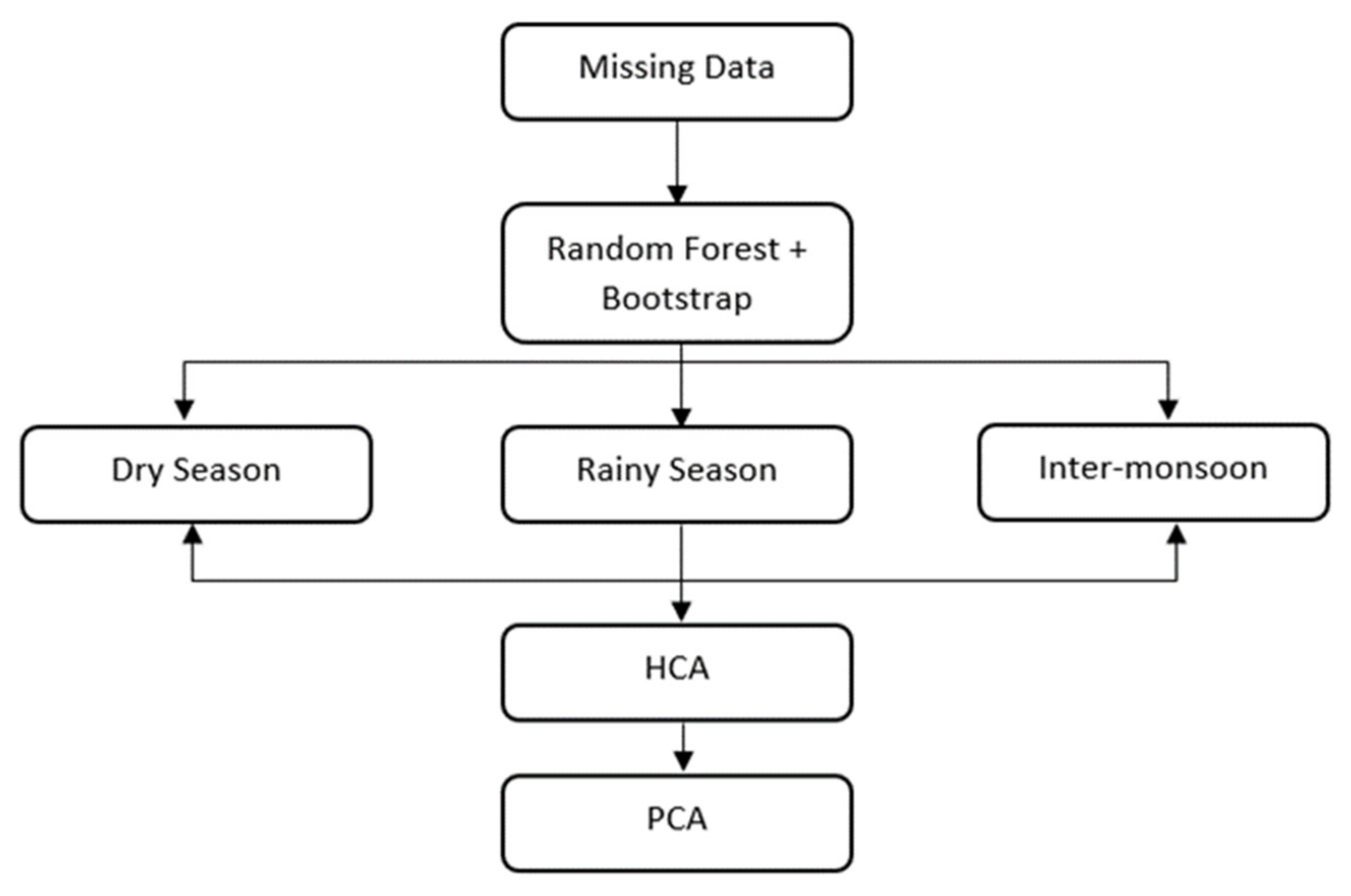
4.3. Statistical Properties of Rainfall Clusters

Cluster-wise statistics of the mean rainfall over season are presented in

Table 2. Statistics for cluster-wise mean rainfall for the seasonal series.

Period	Cluster	Range (mm)	Mean (mm)	Standard Deviation (mm)	Coefficient of Variation (%)	Skewness	Kurtosis
Dry Season	I	0.750–519.750	115.114	106.239	2.37	−0.01	0.20
	II	0.625–524.138	94.015	91.662	2.57	0.06	−0.11
	III	0.250–457.104	77.274	77.925	2.67	0.06	−0.05
	IV	1.000–622.000	138.031	133.933	2.45	0.03	0.37
Rainy Season	I	6.348–1176.000	326.742	151.468	2.41	−0.04	0.17
	II	7.954–1048.625	301.972	163.407	2.70	0.05	−0.09
	III	6.635–837.625	256.219	136.806	2.72	0.08	0.00
	IV	5.940–1190.500	389.521	186.392	2.39	0.04	0.03
Inter-monsoon	I	4.770–602.750	193.492	123.764	2.30	0.12	−0.30
	II	7.864–567.204	159.002	115.514	2.75	0.11	−0.08
	III	3.895–578.090	127.921	104.500	2.68	−0.03	0.05
	IV	6.783–607.250	217.980	139.707	2.29	0.03	0.00

. The mean rainfall remains the lowest in cluster III and the highest in cluster IV for each season. It shows the consistent mean of rainfall by the four clusters. In general, cluster III has a small variation and cluster IV has a large variation for each season in the rainfall recognition patterns. The skewness values for all clusters are within the permissible limits of −0.040 to 0.116 for the distribution of data. The results illustrated that the shape of rainfall distribution for the rainfall stations in the Special Region of Yogyakarta was fairly symmetrical due to the values of the skewness being close to zero. The coefficient of variation was obtained by the closest values between each rainfall patterns for all seasons. Cluster II in the inter-monsoon season showed the largest variability of monthly rainfall amounts, at 2.751%. Meanwhile, the lowest coefficient variation was found in the same season with the variation of 2.285% in cluster IV. Kurtosis represents the tails of the distribution of the data and usually it measures the presence of outliers in the distribution. The high values of kurtosis, which is kurtosis >3, shows that the data have heavy tails and contain outliers, while if the kurtosis <3, the data have light tails and contain a lack of outliers. From Table 2 it clearly shows that all the data in each cluster for all seasons have a lack of outliers due to all the kurtosis values being under 3.

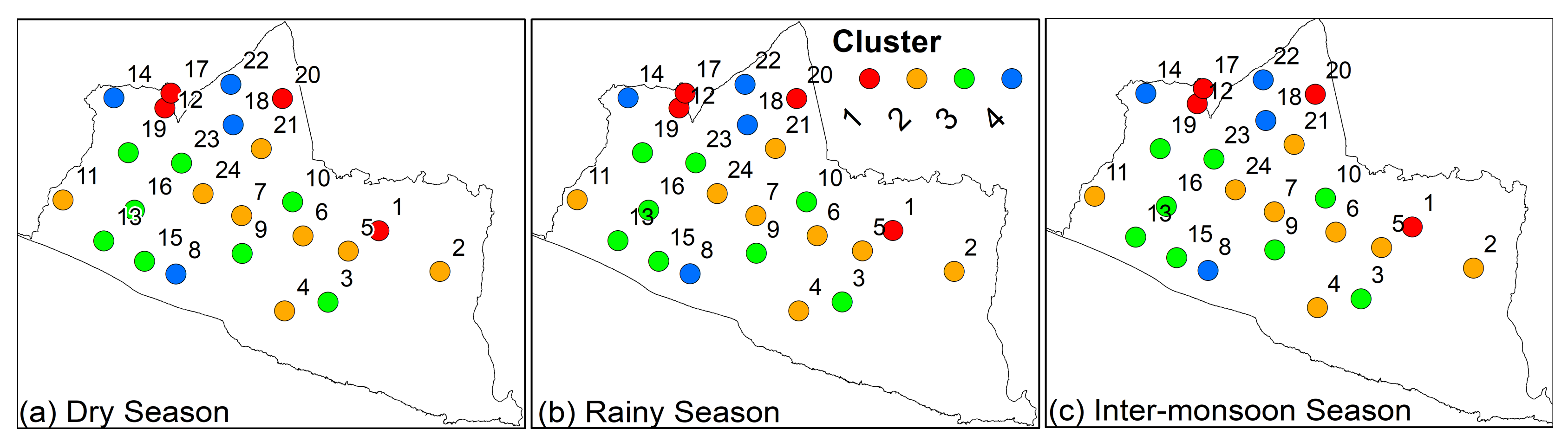
The main features of the clustering results are discussed to verify the distinction between the clusters with respect to their significant locations and the period of monsoon occurrence for the torrential rainfall patterns based on the recommended settings in the previous methodology section. Description of the rainfall patterns refer to range based on Regulation of Head of Meteorology, Climatology, and Geophysics Agency (BMKG), No. KEP.009 of 2010 on Standard Operating Procedures for Implementation of Early Warning, Reporting and Dissemination of Extreme Weather Information [45]. The distributions of seasonal rainfall data are shown in

Table 3. The seasonal rainfall amount within four clusters in a region.

Cluster Region	Cluster	Location	Highest Average Monthly Rainfall Amount (mm)	Rainfall Pattern
Dry Season	Cluster 1	Station 1	98–168	Mild
	Cluster 2	Station 24
	Cluster 3	Station 23
	Cluster 4	Station 22
Rainy Season	Cluster 1	Station 1	284–424	Heavy
	Cluster 2	Station 11
	Cluster 3	Station 16
	Cluster 4	Station 22
Inter-monsoon	Cluster 1	Station 20	170–275	Moderate
	Cluster 2	Station 21
	Cluster 3	Station 23
	Cluster 4	Station 22

.

There are four clusters based on careful examination which reveal that the stations in cluster 1 are marked with a red marking, cluster 2 with an orange marking, cluster 3 with a green marking and in cluster 4 with a blue marking, as shown in Figure 5.

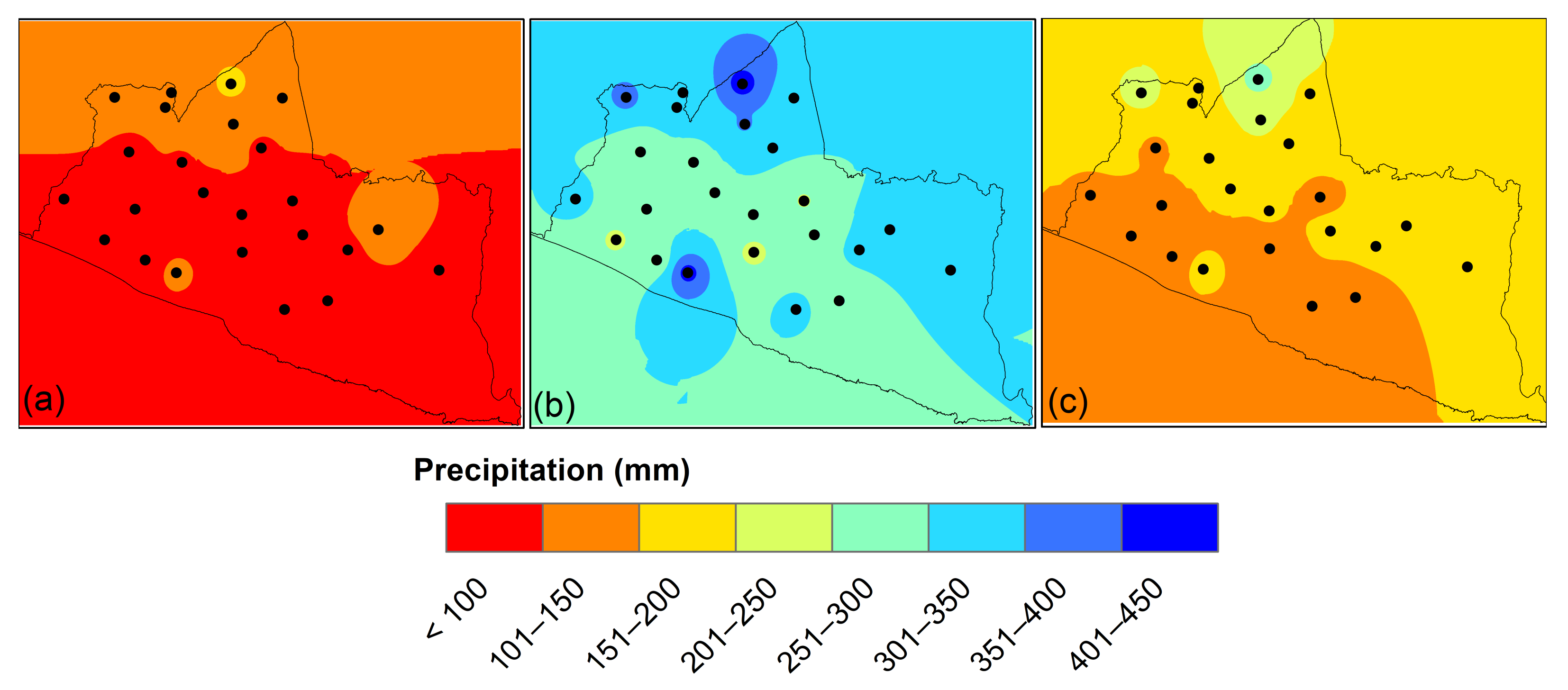
From Table 3, the rainy season produces the highest average monthly rainfall amount, with a range of rainfall from 284 mm to 424 mm, exhibiting heavy monthly rainfall patterns. For the inter-monsoon season, the value of the highest average monthly rainfall amount in the range of rainfall from 170 mm to 275 mm, classifies this season as having moderate monthly rainfall patterns. The dry season has the least rainfall compared to the rainy season and inter-monsoon season, with the range of rainfall being from 98 mm to 168 mm, classifying the season as having mild monthly rainfall patterns.

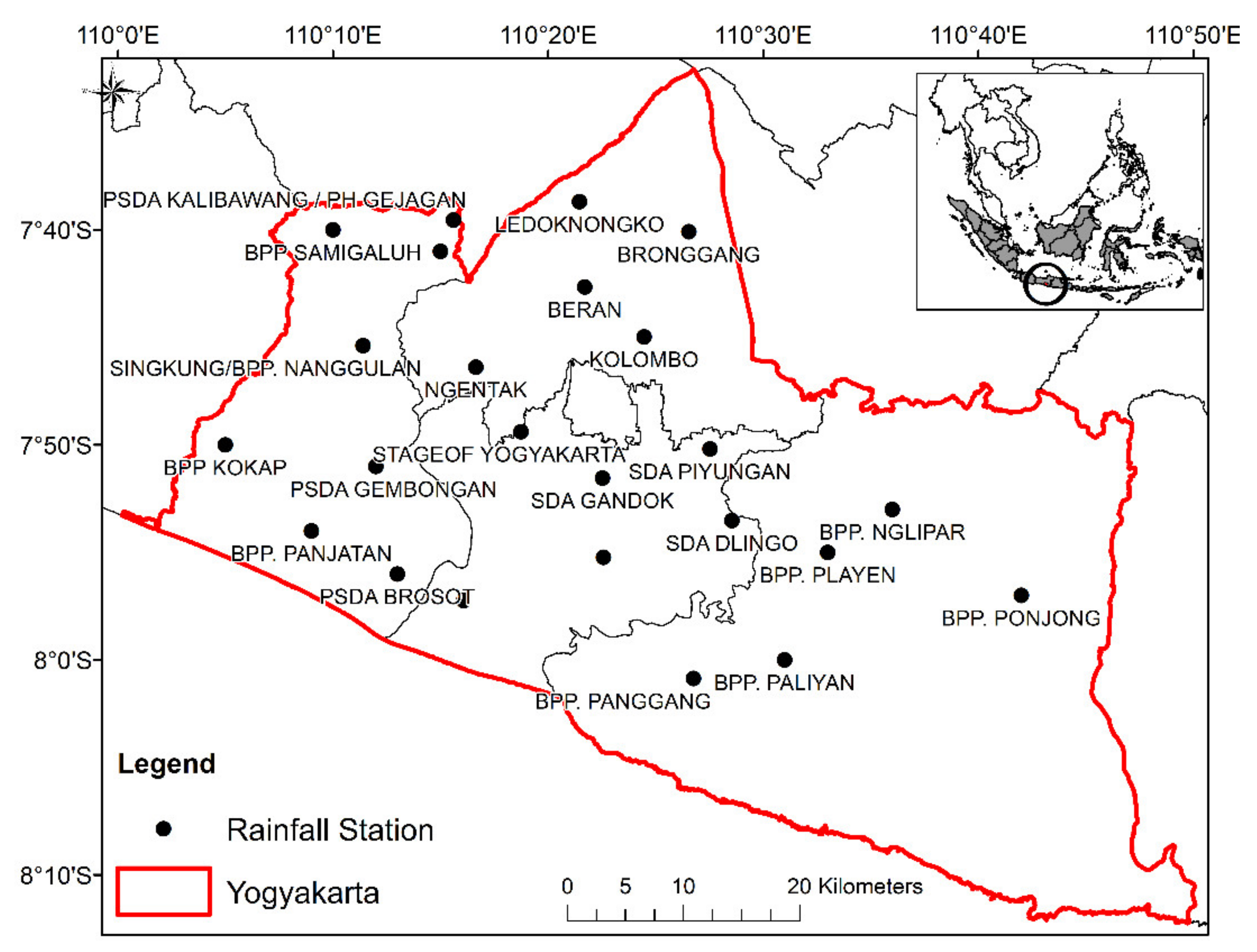
Cluster 1, which is located in the North of Yogyakarta city, shows that the most significant station that produced the highest average monthly rainfall amount is Station 1 for the dry season and the rainy season, while for the inter-monsoon, Station 20 dominates in Cluster 1 for the highest average monthly rainfall amount (Figure 4). Cluster 2, which extends to the southern parts of Yogyakarta city, shows that the most significant station that produces the highest average monthly rainfall amount is Station 24 for the dry season, and Station 11 for rainy season and Station 21 for the inter-monsoon season.

In Cluster 3, the most significant station, which produces the highest average monthly rainfall amount, is Station 23 for the dry season and the inter-monsoon season, while for the rainy season, Station 16 has the highest average monthly rainfall amount. Lastly, in Cluster 4, the most significant station that produces the highest average monthly rainfall amount is Station 22 in every season.

4.4. Cumulative Percentage of Principal Component Analysis (PCA)

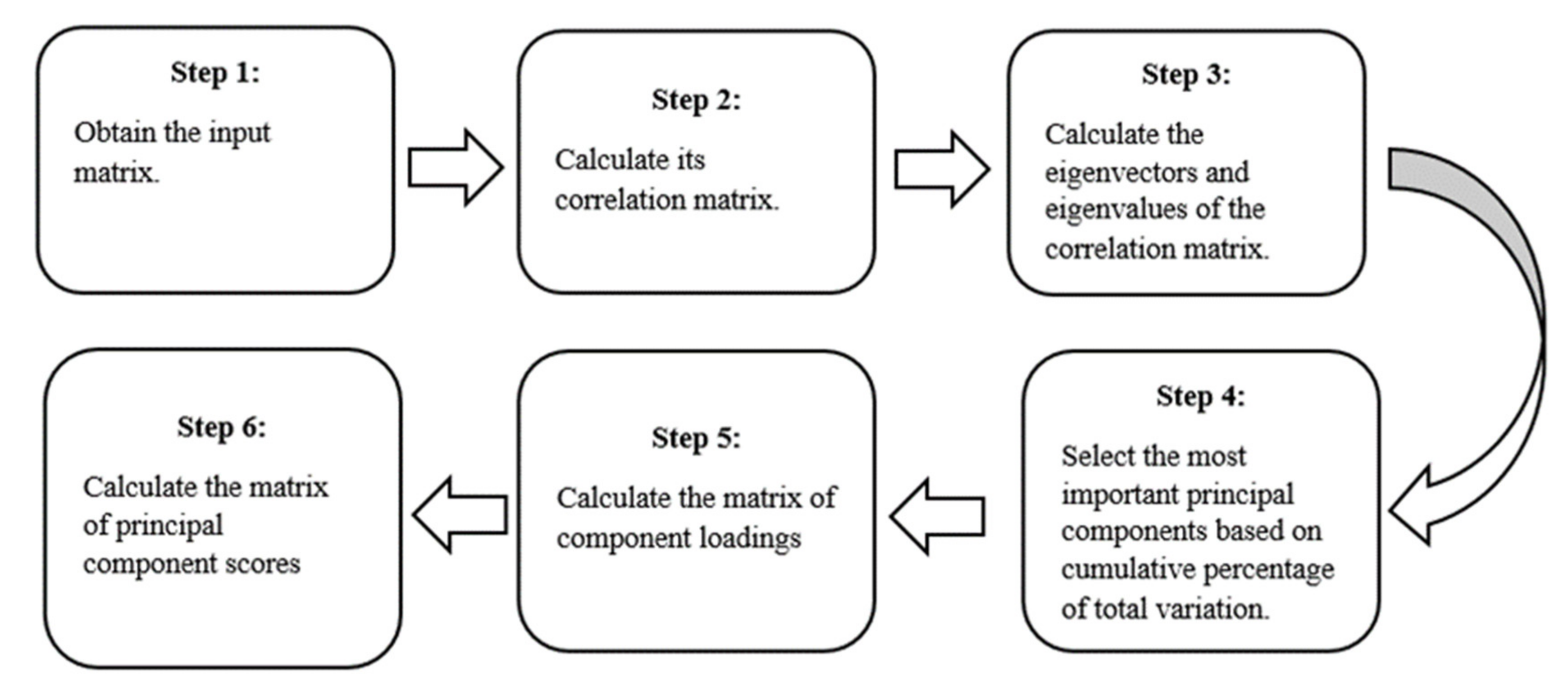
In this section, we will discuss the choice of cumulative percentage to cut off the number of principal components based on the three different seasons. The principal component in this study refers to the new variables that are constructed as linear combinations or mixtures of the initial variables. These combinations are done in such a way that the new variables (i.e., principal components) are uncorrelated and most of the information within the initial variables is squeezed or compressed into the first components.

The monthly average is composed of 12 factors that were analyzed at 75 locations around Thessaly. These variables were found to be linked to each other. Their explanations of the data in terms of a smaller number of uncorrelated variables simplified and structured it in a way that made it easier to comprehend [46]. This is accomplished through the use of Principal Component Analysis. This was accomplished by identifying 12 linear combinations of the original variables, dubbed principal components, that are mutually uncorrelated, and by calculating the proportion of total variance that each of them could account for.

From

Table 4. Summary of the PCA results for eigenvalues, percentage of variation and number of components obtained for each season in Yogyakarta, Indonesia.

		Season
	Eigenvalues	Cumulative Percentage (%)	Number of Principal Component
Dry	1.07	54.55	10
	1.02	58.90	11
	0.97	62.99	12
	0.96	66.83	13
	0.92	70.50	14
Rainy	1.07	54.55	10
	1.05	58.90	11
	0.98	62.99	12
	0.92	66.83	13
	0.88	70.50	14
Inter monsoon	1.14	61.01	10
	1.05	65.37	11
	1.01	69.57	12
	0.93	73.45	13
	0.81	76.81	14

, we can see clearly that the choice of cumulative percentage of variance will reflect the number of components to retain. It appears that all seasons obtained the same number of components at different levels of cumulative percentages of variations. The selection of a higher cumulative percentage of variation has extracted a greater number of components for each monthly rainfall season in the Special Region of Yogyakarta, Indonesia.

For instance, 10 components and 14 components were retained with PCA at more than 50% and 70% cumulative percentage of variation respectively. However, in identifying rainfall patterns, extracting the correct number of components is crucial because it dictates the rainfall days belonging to the correct grouping patterns. The results showed a significant correlation between principal components and stations such as PCA at Bronggang, Beran and Ledoknongko station, which was high due to the higher elevation near Mount Merapi, Nglipar, Playen and Ponjong, which was also at a high elevation and was borderd by a reservoir area. The eastern and western boarders are highland areas, while in the southern part of the station at Panggang, Paliyan, Kokap and Panjatan, there is a low land area near the Indian Ocean. This result is supported by Dai et al. [18], who stated that a lesser number of components would be insufficient to identify rainfall patterns when dealing with analysing considerable new patterns of rainfall in a selected region. Meanwhile, the inclusion of too many principal components inflates the importance of noise and results in poorly identified new cluster patterns [10]. There is no rough guidance for determining the optimal cumulative percentage of variance; however, Jollife [42] proposed that the optimal cumulative percentage for climatic data can be greater than 70%. This was proved from the previous literature [19]. Based on the results in Table 4, the 70% cumulative of variations were obtained by the sufficient components of 14 components for all seasons.

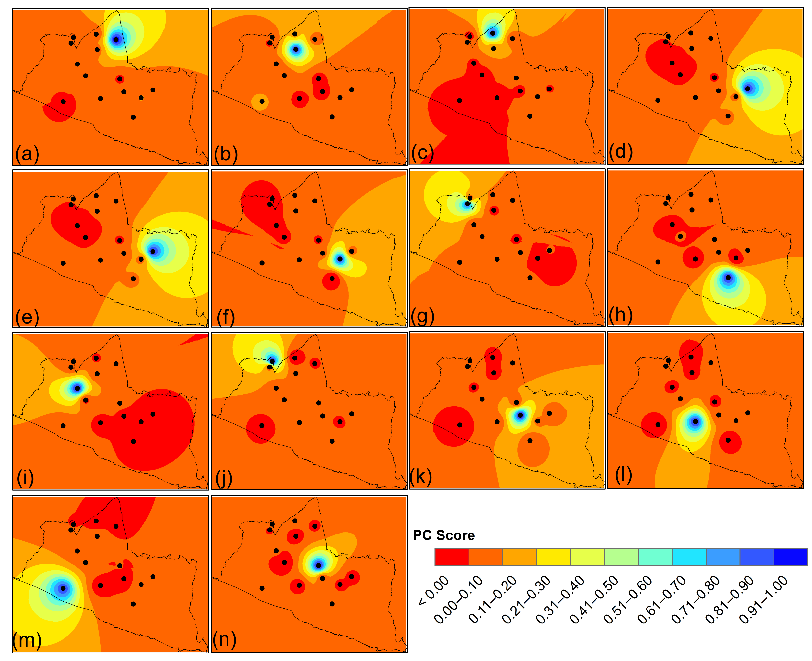
4.5. Principal Component Analysis (PCA)

Every component item and its loadings with a load component over 0.50 was retained in the PCA [19]. Based on

Table 5. Loadings for the first 14 PCs of the Dry Season in Yogyakarta, Indonesia.

Rainfall					Loading
Station	PC1	PC2	PC3	PC4	PC5	PC6	PC7	PC8	PC9	PC10	PC11	PC12	PC13	PC14
NGLIPAR	0.027	0.000	−0.006	−0.033	0.924 *	0.044	0.004	0.067	−0.066	0.038	0.049	0.095	0.081	−0.029
PALIYAN	0.023	0.028	0.034	0.023	0.081	−0.129	0.008	0.919 *	−0.034	0.042	0.001	−0.083	0.015	0.009
PLAYEN	0.107	0.027	0.055	−0.012	0.052	0.879 *	−0.087	−0.135	−0.033	−0.015	0.068	0.003	0.049	−0.035
DLINGO	0.006	−0.027	−0.013	0.014	0.044	0.052	0.070	0.002	−0.017	−0.001	0.964 *	0.011	−0.073	−0.011
NGETAL	0.023	−0.030	−0.051	0.031	0.098	0.017	0.086	−0.066	−0.049	−0.001	0.004	0.931 *	−0.086	−0.054
PIYUNGAN	−0.019	−0.035	0.004	−0.084	−0.024	−0.026	−0.018	0.002	0.009	0.068	−0.010	−0.044	0.003	0.978 *
BPP. KALIBAWANG	0.067	−0.027	0.056	0.042	−0.016	−0.089	0.906 *	0.012	0.026	−0.013	0.104	0.107	0.076	−0.017
BROSOT	−0.031	0.111	−0.082	0.087	0.097	0.066	0.069	0.033	−0.003	−0.057	−0.102	−0.091	0.880 *	0.012
PSDA KALIBAWANG	−0.013	0.047	−0.055	0.043	0.034	−0.013	−0.001	0.035	−0.002	0.972 *	−0.004	−0.006	−0.037	0.071
BERAN	0.062	0.906 *	0.105	−0.007	0.004	0.017	−0.041	0.016	0.006	0.062	−0.031	−0.027	0.095	−0.052
BRONGGANG	0.972 *	0.047	0.018	0.055	0.024	0.077	0.044	0.018	0.020	−0.014	0.007	0.027	−0.014	−0.019
LEDOKNONGKO	−0.006	0.157	0.866 *	−0.050	0.006	0.084	0.085	0.030	−0.017	−0.109	−0.026	−0.062	−0.113	0.034
NGENTAK	0.018	0.005	−0.021	−0.029	−0.056	−0.019	0.013	−0.024	0.981 *	−0.003	−0.014	−0.038	−0.006	0.010
STAGE OF YOGYAKARTA	0.065	−0.002	−0.062	0.910 *	−0.037	−0.018	0.034	0.004	−0.040	0.053	0.023	0.039	0.078	−0.102

* Indicate high loading in PCs.

, one component was retained in PC1 with a load component higher than 0.50: the Station of Bronggang, with a value of 0.972, situated near the hill and on the top of Special Region of Yogyakarta, is the dominant station in PC1. In PC2, the maximum factor loading value of Beran is the dominant station, with a value similar to the BPP.Kalibawang of 0.906. Ledoknongko, PC3, has the maximum load factor with a value of 0.866 near station 20, which is next to two hills. For PC 4, the core of Yogyakarta is Stage of Yogyakarta with the maximum factor loading value of 0.910.

The next PC5 with a dominant station is Station 1, which is situated in the north of the Kulon Progo regency in Cluster 1, with a value of 0.924. Nglipar is superior in PC6, with a factor loading value of 0.879 in the region of Gunung Kidul regency. The highest loading factor rating is PC7, BPP. Kalibawang, with a value of 0.906, is located north of Kulon Progo regency and is close to the hill. The dominant station for PC8 is Paliyan, with a value of 0.919. Ngentak is at 0.981 and its nearest position to Yogyakarta city is the dominant station PC9. The dominant station PC10 is PSDA. Kalibawang, with a value of 0.972, is similar to Bronggang and is located north of the Kulon Progo regency. The dominant station at PC11 is Dlingo, with a value of 0.964, situated close to four hills east of the Bantul regency. The maximum factor loading value of PC12 is 0.931 at Ngetal, which is located in the region of the Bantul regency, south of Yogyakarta city. The dominant station of PC 13 is Brosot, with a value of 0.880, situated near the Indian Ocean. The dominant station of PC14 is Piyungan, with a value of 0.978, situated near the hill east of the Bantul regency.

The largest PC values are found in the north, in the centre of Special Region of Yogyakarta, in the south and east of the Special Region of Yogyakarta, suggesting the highest dry season contribution to overall rainfall. In the northern part of the Special Region of Yogyakarta, strong precipitation in the dry season is attributed to the convective process due to its position close to the hills and the availability of air humidity in the atmosphere, as shown in Figure 6.

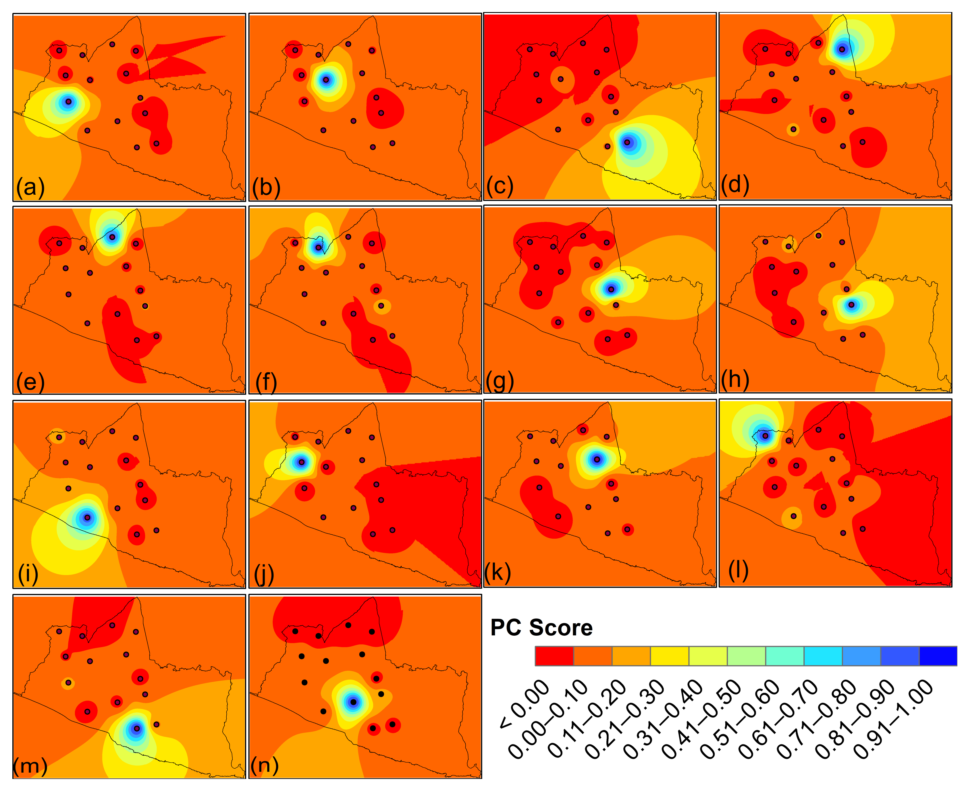
Based on

Table 6. Loadings for the first 14 PCs of the rainy season in Yogyakarta, Indonesia.

Rainfall					Loading
Station	PC1	PC2	PC3	PC4	PC5	PC6	PC7	PC8	PC9	PC10	PC11	PC12	PC13	PC14
PALIYAN	−0.031	0.029	0.934 *	−0.069	−0.003	0.005	−0.030	0.001	0.065	−0.013	−0.008	−0.056	0.081	−0.027
PANGGANG	0.102	0.037	0.081	0.019	−0.025	−0.079	−0.048	0.037	−0.046	−0.011	0.019	0.059	0.937 *	−0.035
DLINGO	−0.067	−0.091	−0.007	0.067	0.112	0.164	0.066	0.871 *	−0.032	−0.085	0.009	0.031	0.056	0.117
GEDONGAN	0.051	0.022	0.098	0.121	0.053	0.085	−0.006	−0.061	0.867 *	0.029	−0.066	0.142	−0.057	0.009
NGETAL	0.018	0.020	−0.025	−0.054	−0.108	−0.058	−0.048	0.081	0.002	0.046	0.026	−0.026	−0.034	0.954 *
PIYUNGAN	0.006	−0.036	−0.027	−0.023	−0.013	−0.023	0.978 *	0.039	−0.006	−0.003	−0.045	−0.004	−0.042	−0.044
BPP. KALIBAWANG	0.046	0.001	0.001	−0.043	−0.004	0.914 *	−0.035	0.137	0.069	0.005	0.018	−0.019	−0.088	−0.065
SAMIGALUH	−0.027	−0.034	−0.064	−0.041	−0.100	−0.029	−0.008	0.043	0.110	−0.023	0.047	0.924 *	0.058	−0.035
GEMBONGAN	0.861 *	−0.025	−0.064	−0.026	0.066	0.005	−0.027	−0.025	0.118	−0.108	−0.068	−0.049	0.120	0.042
SINGKUNG	−0.065	−0.059	−0.018	0.012	0.066	0.013	0.000	−0.060	0.030	0.941 *	0.020	−0.029	−0.005	0.051
BRONGGANG	−0.008	−0.008	−0.077	0.950 *	−0.052	−0.048	−0.027	0.060	0.094	0.015	0.028	−0.043	0.016	−0.061
KOLOMBO	−0.029	0.051	−0.006	0.017	−0.020	0.018	−0.045	0.004	−0.038	0.016	0.974 *	0.034	0.016	0.025
LEDOKNONGKO	0.078	0.096	−0.022	−0.060	0.853 *	0.010	−0.018	0.104	0.037	0.102	−0.036	−0.130	−0.020	−0.166
NGENTAK	−0.012	0.926 *	0.027	0.003	0.076	0.006	−0.036	−0.070	0.020	−0.072	0.067	−0.030	0.043	0.030

* Indicates high loading in PCs.

, the dominant station in PC1 is Gembongan, with a value of 0.861, which is situated next to Indian Ocean and is also located on the southwest of the Special Region of Yogyakarta. The dominant station of PC2 is Ngentak, with a value of 0.926, which is situated in the lower part of the Bantul regency and close to the Indian Ocean. The dominant station for PC3 is Paliyan, with a factor loading value of 0.934. The dominant station of PC4 is Brongang, near the hill and on the top of the Yogyakarta city, with a value of 0.950. For PC5, the dominant station is Ledoknongko, with a factor loading value of 0.853 and its position is next to Bronggang, which is close to two hills. The dominant station of PC6 is BPP. Kalibawang is situated on the north side of the Kulon Progo regency and is close to the hill, with a value of 0.914.

The dominant station in PC7 is Piyungan, located to the east of the Kulon Progo regency and close to the hill, with a factor loading value of 0.978. The dominant station for PC8 is Dlingo, with a factor loading value of 0.871, situated near four hills east of the Bantul regency. The dominant station in PC9 is Gedongan, with a value of 0.871, positioned close to the city of Yogyakarta. PC10, Singkung, with a value of 0.941, is the dominant station. The dominant station PC11 is Kolombo, which is situated near to Yogyakarta city in the south of the Sleman regency. The dominant station of PC12 is Samigaluh, with a factor loading value of 0.924 on the north side of Kulon Progo regency and close to two hills.

The dominant station of PC13 is Panggang, with a value of 0.937, and is situated south of the Gunung Kidul regency near the Indian Ocean. The dominant station in PC14 is Ngetal, with a factor loading value of 0.954, situated south of the Bantul regency, close to station 23 and near the Indian Ocean. The spatial view of the PC score represented by the Special Region of Yogyakarta region stations reveals that the eastern part of the Special Region of Yogyakarta indicates low rainfall precipitation due to no stations serving in that area. The positive meaning of the PC is in the north, south, and southwest, and in the centre of Yogyakarta as shown in Figure 7. It indicates that the southern portion is closed to the Indian Ocean during rainy seasons, to the north side of the Special Region of Yogyakarta, and to the center of the Special Region of Yogyakarta, which is closed to the city of Yogyakarta and has the maximum rainfall precipitate.

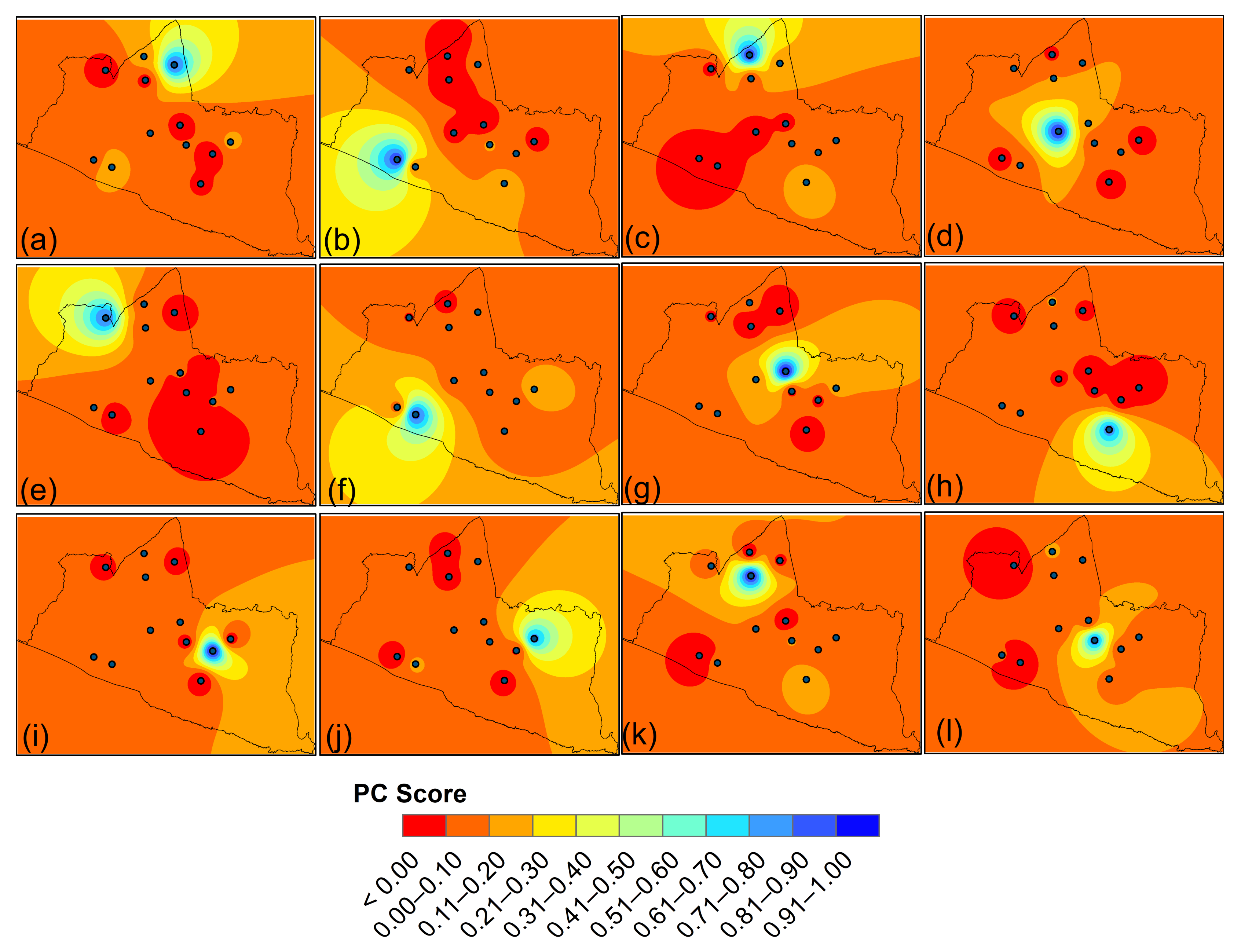
Based on

Table 7. Loadings for the first 12 PCs of the inter-monsoon season in Yogyakarta, Indonesia.

Rainfall					Loading
Station	PC1	PC2	PC3	PC4	PC5	PC6	PC7	PC8	PC9	PC10	PC11	PC12
NGLIPAR	0.127	−0.036	0.009	−0.041	0.020	0.133	0.117	−0.085	−0.058	0.755 *	0.016	0.055
PALIYAN	−0.010	0.138	0.172	−0.045	−0.018	0.057	−0.077	0.766 *	−0.102	−0.053	0.152	0.068
PLAYEN	−0.062	0.085	0.092	0.016	0.003	0.082	−0.023	−0.092	0.970 *	−0.023	0.045	−0.008
DLINGO	0.001	0.115	0.086	−0.003	−0.160	0.005	−0.040	−0.022	−0.053	0.050	0.109	0.793 *
GANDOK	0.086	−0.040	−0.077	0.943 *	0.024	0.031	0.110	−0.009	0.016	0.017	0.077	−0.001
GEDONGAN	0.136	0.109	−0.057	−0.001	−0.024	0.856 *	0.070	0.016	0.070	0.121	0.030	−0.079
PIYUNGAN	−0.068	−0.077	−0.037	0.104	0.012	0.050	0.987 *	−0.024	0.000	0.094	−0.092	−0.022
BPP. KALIBAWANG	−0.071	0.083	−0.026	0.015	0.811 *	−0.003	−0.003	−0.033	−0.021	0.037	0.055	−0.139
BROSOT	0.080	0.897 *	−0.071	−0.034	0.022	0.054	−0.003	0.064	0.058	−0.045	−0.111	0.005
BERAN	−0.043	−0.108	0.004	0.102	0.014	0.027	−0.066	0.054	0.027	−0.033	0.932 *	0.047
BRONGGANG	0.838 *	0.045	0.125	0.099	−0.056	0.103	−0.090	−0.017	−0.038	0.061	−0.028	0.047
LEDOKNONGKO	0.131	−0.079	0.890 *	−0.024	0.041	−0.032	0.013	0.108	0.101	−0.038	−0.072	0.117

* Indicates high loading in PCs.

for PC1, the dominant station is Bronggang, with a load factor value of 0.838. It is located on the north side of the city of Yogyakarta and the Sleman regency. The dominant station of PC2 is Brosot, with a value of 0.897, situated near to the Indian Ocean. For PC3, the dominant station is Ledoknongko, situated near Bronggang, which is next to two hills. The dominant station for PC4 is Gandok with a load factor value of 0.943. Station 7 is located in the centre of Bantul regency. The dominant station for PC5 is BPP. Kalibawang, positioned north of the Kulon Progo regency and close to the hill, with the factor loading of 0.811.

The dominant station, PC6, is Gedongan, with a value of 0.856, near to the city of Yogyakarta. Piyungan, with a factor loading value of 0.987, is the dominant station for PC7 and is situated east of the Kulon Progo regency and close to the hill. For PC8, the prevailing station is Paliyan, with a load factor of 0.766. On the west side of the Gunung Kidul regency, PC9, the dominant station is Playen with a factor loading of 0.970. PC10, the dominant station, with a value of 0.755, is in Nglipar, situated north of the Kulon Progo regency. The dominant station of PC11 is Beran, with a factor loading value of 0.932, and its position is near to the city of Yogyakarta. The dominant station PC12 is Dlingo, with a load factor of 0.947 and its position is near four hills east of the Bantul regency.

There is greater rainfall during the season on the north side of Yogyakarta city. The station has represented the positive PC score during the inter-monsoon season, indicating that the region with heavy precipitate rainfall is in the north, the center of the Special Region of Yogyakarta and on the east side, as shown in Figure 8. The southern region that is closed to the Indian Ocean represents just two stations.

5. Conclusions

This study proposed a hybrid imputation approach using RF-Bs combined with multivariate analysis to identify patterns of spatial rainfall across Yogyakarta, Indonesia. Enhancements in imputing methods of RF-Bs in filling the long gap for monthly rainfall datasets potentially could be used for regionalization of rainfall regimes in the Special Region of Yogyakarta, Indonesia. Rainfall regimes were regionalized for the Special Region of Yogyakarta, Indonesia, by using Principal Component Analysis with varimax rotation based on three sets of seasonal monthly rainfall data during the years 1970 to 2019. Fourteen and twelve principal component analyses for dry, rainy and inter-monsoon seasons were extracted based on a cumulative percentage of variation data. All the significant rotated components, which explain more than 70% of the total variance in the data, were used to calculate the PC loading. According to the results, the main rainfall is in the dry season. In some parts of northern and southern of Yogyakarta, more than half of the total precipitation occurs in the dry season. Moving away from the mentioned regions to the Indian Ocean, the contribution of the rainy season to the rainfall total becomes higher than the rainfall in the dry and inter-monsoon seasons. The rainfall in the north-west and south-east parts of the Special Region of Yogyakarta is classified as being from the dry season. The contribution of inter-monsoon season rainfall to the total rainfall amount is noticeable in the city of Yogyakarta and in the eastern parts of the Special Region of Yogyakarta and in northern areas. By applying hierarchical cluster analysis on monthly rainfall data, about four homogenous rainfall regimes were identified for each season. According to the results, the use of the dataset in order to group rainfall regimes is recommended for the tropical region, especially for the whole region in Indonesia, while its utilization in the wet and dry regions needs to be further studied in the future.