
Using Machine Learning to Map Western Australian Landscapes for Mineral Exploration


CSIRO Mineral Resources, Australian Resources Research Centre, 26 Dick Perry Ave., Kensington, Perth, WA 6151, Australia
*
Author to whom correspondence should be addressed.
ISPRS Int. J. Geo-Inf. 2021, 10(7), 459; https://doi.org/10.3390/ijgi10070459
Submission received: 25 April 2021
/
Revised: 23 June 2021
/
Accepted: 24 June 2021
/
Published: 6 July 2021
Abstract
:Landscapes evolve due to climatic conditions, tectonic activity, geological features, biological activity, and sedimentary dynamics. Geological processes at depth ultimately control and are linked to the resulting surface features. Large regions in Australia, West Africa, India, and China are blanketed by cover (intensely weathered surface material and/or later sediment deposition, both up to hundreds of metres thick). Mineral exploration through cover poses a significant technological challenge worldwide. Classifying and understanding landscape types and their variability is of key importance for mineral exploration in covered regions. Landscape variability expresses how near-surface geochemistry is linked to underlying lithologies. Therefore, landscape variability mapping should inform surface geochemical sampling strategies for mineral exploration. Advances in satellite imaging and computing power have enabled the creation of large geospatial data sets, the sheer size of which necessitates automated processing. In this study, we describe a methodology to enable the automated mapping of landscape pattern domains using machine learning (ML) algorithms. From a freely available digital elevation model, derived data, and sample landclass boundaries provided by domain experts, our algorithm produces a dense map of the model region in Western Australia. Both random forest and support vector machine classification achieve approximately 98% classification accuracy with a reasonable runtime of 48 minutes on a single Intel® Core™ i7-8550U CPU core. We discuss computational resources and study the effect of grid resolution. Larger tiles result in a more contiguous map, whereas smaller tiles result in a more detailed and, at some point, noisy map. Diversity and distribution of landscapes mapped in this study support previous results. In addition, our results are consistent with the geological trends and main basement features in the region. Mapping landscape variability at a large scale can be used globally as a fundamental tool for guiding more efficient mineral exploration programs in regions under cover.
1. Introduction
1.1. Geomorphology Background
The overall increase in demand for commodities to support a growing population is a powerful driver for mineral exploration. Large surface areas of the continents are covered by intensely weathered surface material and/or sediment deposition, such as in Australia, West Africa, India, and China [1]. Exploration through this cover is becoming one of the fundamental challenges for the minerals industry in this century.
Landscapes contain essential information related to the geochemical footprint of ore deposits at depth (e.g., [2,3,4]). Variable surface topographical features can be grouped to define and classify unique landscape domains. Climatic conditions, tectonic activity, geological features, biological activity, and sedimentary dynamics are fundamentally linked to landscape evolution and its diversity (e.g., [5]). Consequently, the study of landscapes can link surface features to geological processes at depth. Ore deposits and mineral systems can have dispersed and enhanced geochemical footprints due to landscape evolution (e.g., [3,6,7], and references therein). Geochemical dispersion halos through the cover can be detected by selecting suitable landscape regimes and appropriate sample media (e.g., [8,9,10,11,12,13,14,15]).
Cataloguing landscape differences and evolution at a regional scale can be challenging. The primary difficulty is associated with the selection of the geographic extension of surficial features. Field observations have been relied upon to understand landscape diversity. However, a constraint on this approach lies in the uncertainty related to the extrapolation of field observations, especially when attempting to extrapolate them to regional scales. Such extrapolation can be unreliable due to the complexity and variability of landforms, the paucity of data availability, and the difficulty in defining quantitative criteria that discriminate diverse landscape types. Modern data analytics technology and advanced satellite imaging provide access to large data sets that can assist in characterising landscape features and their distribution at regional scales. The ability to accurately map landscape domains enhances the ability to link surface geochemistry with the geology at depth.
The landscapes of Western Australia are characterised by low topographic relief and a deeply weathered blanket that covers most of the state. This landscape context is challenging for mineral exploration due to the lack of fresh rock exposure at surface. However, domain experts have identified distinct landscape variability that changes imperceptibly at small scales. Landscape evolution may record geochemical and stratigraphic information that link the basement and the surface (e.g., [5,11,16,17,18,19]). The integration of landscape evolution and surface geochemistry in deeply and intensely weathered regions is a fundamental tool in mineral exploration used around the world (e.g., [2,6,7], and references therein).
Landscapes are defined by their surface features, such as landforms, vegetation, slopes, sedimentary systems, soils, etc. [20]. The variability of these features allows landscapes to be differentiated from one another, which facilitates classification. From a geological perspective, landscapes are fundamentally linked to: (i) climatic conditions, which control, for example, water availability and weathering processes; (ii) tectonic activity, a main driver of the evolution of surface elevation, which also has a significant impact on sedimentary dynamics and erosional processes; and (iii) geological features, such as structures and lithologies, which control the architecture and variability of the land at surface and at depth [5,16,17,18,19]. Consequently, studying landscapes can reveal the link between surface features and geological processes at depth. In this work, we explored the question of whether these subtle differences between landscape types in low-relief and intensely weathered regions can be quantified on a regional scale, using machine learning approaches, with only desktop compute power.
With this paper, we aim to provide a useful tool for mineral exploration in areas of cover. The innovation presented in this paper comprises the mapping of landscape variability types at a large scale in a covered region, where mineral exploration is highly challenging. The outputs of this research allow for the classification and fine tuning of mineral exploration protocols in such regions to improve sample media selection strategies and more successfully interpret surface geochemical data. The methodology described in this paper can be implemented in other similar regions globally to assist mineral exploration for any commodity (e.g., Au, Ni, etc).
1.2. Overview of Technologies Using Remote Sensing Data for Landscape Mapping
For small scales of approximately 10 km, a wide variety of quantitative methods have been developed in geomorphology ([21,22,23,24,25], and references therein). Others have applied quantitative methods successfully at a regional and continental scale (e.g., [26,27,28]). The difficulty lies both in identifying features that can be used to differentiate landscapes into different domains and in using those features to determine the geographic extent of the domains. This problem is exacerbated in a setting where landscapes are difficult for the untrained eye to distinguish, as is the case of the deeply weathered landscapes of Western Australia.
One of the most challenging aspects of landscape study is cataloguing their differences at regional or even continental scale (e.g., [29]). Integrating data from observations on large scales is an important problem also outside of mineral exploration (e.g., [30]). The difficulty lies not in identifying features that can differentiate landscapes into different domains but also in using those features to determine the geographic extension of the domains. Field observations have been crucial to understand landscape diversity at the regional scale [11]. However, field observations are practically limited to the immediate vicinity of roads, and hence are inherently linear, and any attempt at extrapolating to regional scale introduces significant uncertainty. Such extrapolation suffers from the complexity and variability of landforms and the difficulty in defining quantitative criteria that discriminate diverse landscape types.
Advances in satellite imaging and computing power have enabled the creation of huge yet accessible geospatial data sets. These data sets can assist in characterising landscape features and their distribution at regional scales (e.g., [31,32,33]), which directly impacts many disciplines, including mineral exploration, geomorphology, environmental studies and geoarchaeology, among others (e.g., [2,6,7,34]). Moreover, combined with the drive toward ML in recent years, such data sets have enabled a data-driven approach to automatic landscape classification, without explicitly deriving a specific metric first. Presented with a set of labeled data, an ML classifier learns how to distinguish between classes and can then predict labels for unseen data. Support vector machine and random forest classifiers typically produce the most accurate results. State-of-the-art in the field of computer vision, deep convolutional neural networks (DCNNs) are becoming more common in geology as well. DCNNs implicitly aggregate data, require little to no feature engineering [35], and classification accuracy often exceeds 90%. However, training is computationally expensive.
Classification for mapping purposes is naturally based on spatial input data, which lends itself to either a pixel or an object approach [36]. Conceptually simple, the pixel approach directly feeds pixel values into ML. However, since a pixel is a largely arbitrary region from a geographical point of view, the pixel approach is typically less accurate as it disregards spatial context.
By contrast, an object is a geographically meaningful region and therefore respects natural borders (e.g., roads, for urban mapping). Pixel values from such a region are aggregated before being fed into the ML classifier, preferably in a way that preserves spatial context. This aggregation may improve accuracy, but it is more complex to implement.
Most studies of land cover/land use classification or urban mapping use the pixel approach, and typically achieve accuracies of 80%–90%, sometimes 95%. Lidberg et al. [37] showed that ML outperforms previously used single thresholds when creating high-resolution wet area maps. They reported an overall accuracy of 84% for RF and artificial neural networks (ANNs), followed by 82% for SVM, as compared to 79% for single-threshold classification.
Maxwell et al. [38] compared the performance of six ML classifiers for an agricultural and an urban land cover data set, and reported 89.1% accuracy for SVM and 87.1% for RF. Feature selection (picking only the most important features) increased accuracy to 94.4% for SVM, while decreasing that for RF to 87.8%. They also recommend that, “if possible, the analyst should experiment with multiple classifiers to determine which provides the optimal classification for a specific classification task.” Similarly, Abdi [35] compared SVM, RF, extreme gradient boosting, and DCNNs for land cover and land use classification in a boreal landscape. SVM performed best in his study; however, all approaches yielded similar accuracies in the range of 73%–76%. For urban mapping, Zhang et al. [36] combined remote sensing data and social sensing data, and reported 78% accuracy using a random forest classifier. Fouedjio and Klump [39] investigated the influence of spatial autocorrelation on predictions by random forest and benchmarked them against kriging, which is used more conventionally as a geostatistical technique in mineral resources exploration.
An interesting approach that fits the landscape mapping category, but which does not make use of canonical ML classifiers, is that of Jasiewicz et al. [27,40]. They first computed a signature for a local region (e.g., a px block) called a scene. Then, they computed the distance between scene signatures. Their library provides several signature functions and distance metrics. “Being able to quantify the overall similarity between two landscapes using a single number is a key element” of their work, which allowed them to use averaging for classification resulting in excellent run-time performance. Furthermore, how their algorithm makes decisions can also be easily reproduced and validated by a human. However, reducing landscape complexity to a single dimension inevitably leads to some information loss. In connection with the various averaging steps employed in their methodology, this may or may not be critical. They do not report any accuracy metric.
The literature suggests that landscape mapping algorithms based on classic ML are often less accurate than those using DCNNs, perhaps because most studies follow the pixel approach, i.e., they do not aggregate pixel values prior to classification. Our goal was to implement an algorithm that (1) performs comparably to ANNs/DCNNs (i.e., accuracy ≥90%), but is based on classic ML methods for which training is cheap; (2) is open source, written in a modern language, and, therefore, is easily extendable; and (3) can potentially be run in parallel, enabling processing on a continental scale.
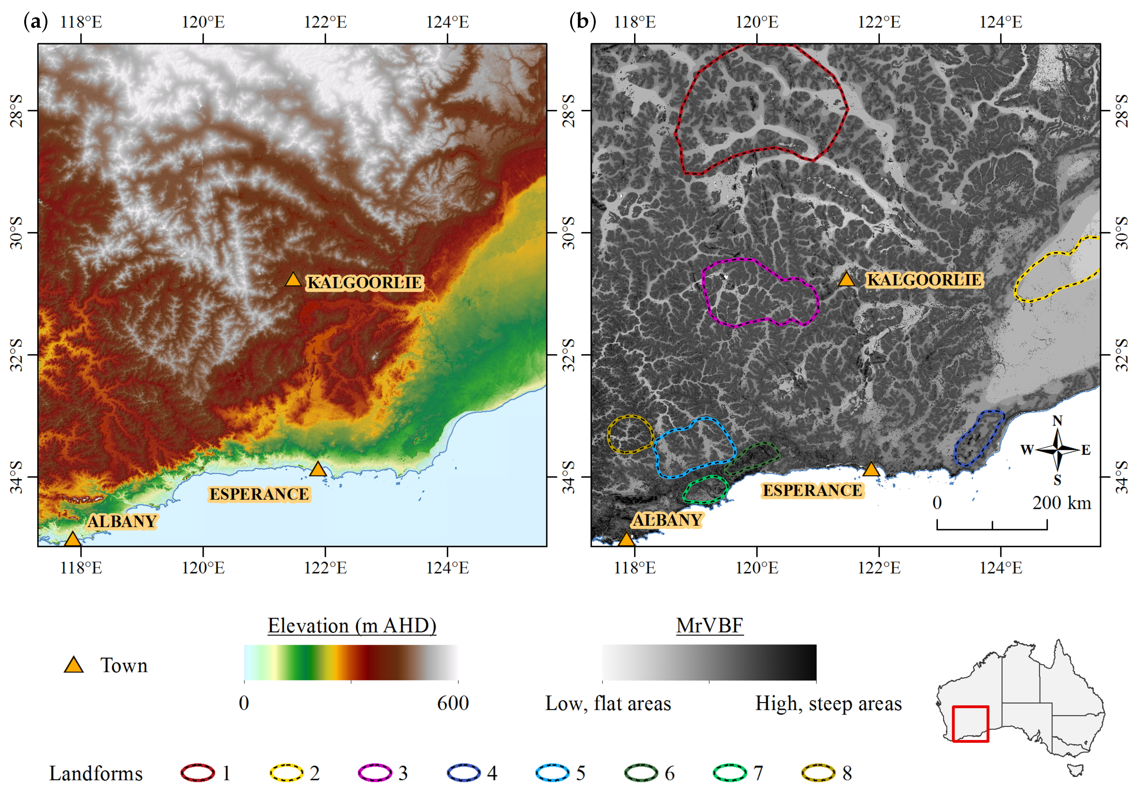
We apply our algorithm to a region of approximately in the south of Western Australia (see Figure 1). Inputs are a freely available (licensed under the terms of the Creative Commons Attribution 3.0 Australia license) digital elevation model (DEM) from Geoscience Australia [41] along with derived data, with sample landclass boundaries provided by domain experts. Our algorithm then produces a dense map of the model region.
In the following section, we review a general ML workflow and detail our methodology. In Section 3, we study how tile size affects classification accuracy and demonstrate a number of extensions that may improve accuracy or provide additional functionality. Discussion and conclusion are presented in Section 4.
2. Methods
2.1. Machine Learning
Traditionally, for a computer to solve a problem, a series of instructions are explicitly programmed, largely of type “if this, do that”, tailored to said problem. In ML, instead of explicit programming, a model is trained. One method of training is to provide known input data along with known sound decisions. After successful training, the model is able to make sound decisions from new, unseen data. This method is known as supervised learning and is what we employed in this paper. The main advantage over explicit programming is that ML models can learn complex relationships between data and decisions (provided enough training data is available), which otherwise would require a human to implement, thereby avoiding costly and error-prone algorithm develoment. Even worse, said relationships may not even be known, rendering explicit programming impossible.
The main advantage over explicit programming is that ML models can learn complex relationships between data and decisions (provided enough good training data is available), which otherwise would require a human to implement similarly complex—hence, costly and error-prone—algorithms. Even worse, said relationships may not even be known, rendering explicit programming impossible.
A general ML workflow includes three main steps: (i) preparing the source data, i.e., selecting data that is relevant to the problem at hand, and transforming it into a format suited for (ii) training a model, followed by (iii) predicting new, unseen data [43]. Machine learning methods can be split into two approaches: supervised and unsupervised learning. Supervised learning requires labeled data on which a model can be trained; such labels are usually provided by a human domain expert. Unsupervised learning requires no labels; one goal could be to detect clusters—i.e., groups with similar features—within the data. We limit this study to supervised learning, but note that an extension to unsupervised learning is straightforward.
Our task is classification: predicting a label for a sample, given a set of features. As labels, we chose arbitrary integers that uniquely identify the eight landforms indicated in Figure 1. We have tested a number of classification methods, namely (i) support vector machine classifier with linear and radial basis function kernels, denoted SVC-LIN and SVC-RBF [44,45]; (ii) decision trees (DT, [46]); and (iii) random forests, consisting of 100 or 1000 Decision Trees (RF-100 and RF-1000, [47]), all accessed via their Python wrappers in scikit-learn [48]. Implemented in Python 3.7, our code is available at https://gitlab.com/fgradi/lpr/. This paper is based on the code dated 1 July 2021.
2.2. Data Preparation: Assembling the Feature Matrix
Many fundamental ML algorithms are designed to operate on a so-called feature matrix. Each row in this matrix corresponds to a sample of the quantity we want to predict. In our case, a sample is the smallest spatial unit that gets assigned a landclass label. We call these units “tiles” (cf. Figure 2), and chose square tiles with side lengths ranging from 51 to 1001 px ( to 86 km). Columns represent features: attributes of a tile which we think are relevant for its classification, e.g., slope or flatness. Assembling the feature matrix from our source data is the major and first of the three steps of our ML approach, described in detail below.
Since the task is 2D pattern recognition and classification, it is crucial that (some) spatial context is preserved during this step. In initial exploratory analysis, we applied principal component analysis to the feature vectors for each pixel, with each pixel treated as an independent observation, and with no consideration of the spatial correlation between nearby pixels. When the pixel data were projected onto the principal components, we found that the component scores did not cluster according to the landscape classes, and the resulting map (not shown) was inaccurate and noisy. This approach produces a large feature matrix, which increases memory requirements.
A more viable approach is spatial aggregation of our source data, but in a way that preserves variation of features typical for a particular landscape class. Simple averaging does not work, as it smooths out those variations, leaving little to distinguish between classes. Instead, we decompose the data into tiles as shown in Figure 2 and compute per-tile normalised histograms of source data. Tiles may overlap, and tile size s and stride r can be specified. Treatment then depends on the type of numerical input, which is either nominal, ordinal, or integer/real. Integer and real data have both ordering () and distance (). Nominals have neither, e.g., “sunny”, “overcast”, “rainy”. Ordinals have an ordering, but no notion of distance: “cold” < “warm” < “hot”. For nominals, within each tile, we calculate the fraction of each area that is equal to a possible value. For ordinals, treat as nominals except using ≤ instead of = on each possible value. For integers and reals, discretise, then treat, as for ordinals.
Nominal or ordinal source data with n possible values results in n features. For integers and reals, the chosen discretisation determines the number of features generated. For example, the slope relief classification source data consists of six slope classes of ordinal type, ranging from “level” to “very steep”. We generate six slopeX features, each value being the fraction of a tile that has the corresponding slope relief classification.
Table 1 summarises all 37 features. We do not use the DEM directly as we aim to classify shape, not elevation. We do, however, include basic statistics of the DEM as features, such as skewness, kurtosis, and interquartile range. Normalising the data is useful as some ML algorithms are not scale invariant, i.e., they perform poorly if some features range, e.g., from 0 to 1 while others range from 0 to 100. The code is designed to make adding additional features straightforward. For example, one could easily include adjacency information, as is done in [27].
The histogram approach has a number of advantages: (i) tile size directly controls the spatial scale of classification, (ii) model training is comparably cheap, potentially enabling continent-scale classification, (iii) classification is invariant under 90 degrees’ rotation, (iv) implementation is reasonably straightforward, and (v) how the algorithm decides can be easily validated by a human. Convolutional neural networks provide an alternative approach, and their applicability to landscape pattern recognition could be explored in the future.

Table 1.
Source data set, data type, and range of a total of 37 features. Most features are generated by computing normalised histograms (NH); some are simple statistics such as mean, skewness, and kurtosis.
Table 1.
Source data set, data type, and range of a total of 37 features. Most features are generated by computing normalised histograms (NH); some are simple statistics such as mean, skewness, and kurtosis.
| Data Set | Data Type, Min…Max, Features | Source |
|---|---|---|
| Geosciences Australia 3″ SRTM DEM v01 | integer, , skewness, kurtosis, interquartile range (IQR) | [41] |
| Multiresolution Valley Bottom Flatness (VBF) | ordinal, , normalised histogram (NH), 10 bins | [42] |
| Multiresolution Ridge Top Flatness (RTF) | ordinal, , NH, 10 bins | [49] |
| Topographic Wetness Index derived from 1″ SRTM DEM-H (TWI) | real, , mean | [50] |
| Slope derived from 1″ SRTM DEM-S | degrees, , skewness, kurtosis, IQR | [51] |
| Wind Exposition Index (WEI) | real, , mean, skewness, kurtosis, IQR | [52,53] |
| Slope Relief Classification derived from 1″ SRTM DEM-S | nominal, six slope codes (see Table 2), H, six bins | [54] |
Table 2.
Slope codes used by [54].
Table 2.
Slope codes used by [54].
| LE | level |
| VG | very gently sloping |
| GE | gently sloping |
| MO | moderately sloping |
| ST | steep |
| VS | very steep |
2.3. Training, Cross-Validation, Prediction
Once the feature matrix is assembled, we train a number of ML models.
Table 3 shows the number of training samples per class. Class 8 has almost 10,000 samples, whereas class 7 has only 560. This is a consequence of the difference in extent of a land class, and scale over which their features vary, cf. Figure 1: class 8 in the NW of our study area covers a vast area of several hundreds of kilometres, whereas class 7 covers only some tens of kilometres. To address this imbalance, we analyse both overall accuracy (defined as the number of correct predictions divided by the total number of predictions) and per-class accuracy.
Initially, we estimated accuracy by tenfold cross-validation: Our labeled data is decomposed into ten equal-sized subsets. A model is trained using nine of these, and its performance is tested on the remaining subset. Repeating this process for different subsets yields ten accuracy estimates, the mean of which we refer to as cross-validation accuracy. Accuracy may be affected by the choice of hyperparameters, i.e. parameters that are unrelated to the training data, and which can be tuned during training. The hyperparameter space is typically small enough such that a simple grid search is feasible. Once we are satisfied with model performance, we train the final model using the entire training data set, and then use it to predict a map.
As an alternative to cross-validation accuracy, one can evaluate accuracy post-training, i.e., based on said final prediction, for all tiles for which the ground-truth is known. However, this is usually considered bad practice, since accuracy would be based entirely on the same data that the model has been trained on.
In our case, however, it was cross-validation accuracy that proved problematic. For tile sizes larger than 17 km, cross-validation accuracy would often approach 100%, whereas post-training accuracy for the same model was much lower, indicating overfitting. This discrepancy is due to the fact that the grids we use for training are, in general, offset from the one on which we predict the final map, as shown in Figure 2c. For training, we extract a block of pixel data defined by the axis-aligned minimum bounding box of a landclass, then decompose that block into tiles (gray grid). The grid for predicting the final map (black), however, is defined by the extent of the input DEM. While aligning both grids would be trivial, we chose not to, as this mismatch helps detecting models that are overly grid-dependent, i.e., overfitted. Post-training accuracy was almost always lower than cross-validation accuracy. We therefore chose to report only the conservative estimate of post-training accuracy, referred to as ”accuracy“ below.
2.4. Computational Cost
In this section, we report the computational cost in terms of aggregation, training, and prediction CPU time, as well as memory requirements. All processing was carried out on an Intel® Core™ i7-8550U CPU notebook with 16 GB RAM.
Our test region extends from (117.2896, −26.8996) deg to (125.6246, −35.1346) deg, covering 794.2 × 915.7 km2. At 3 arc seconds resolution, raster images have a size of 10,002 × 9882 px2. Decomposition into overlapping tiles using a constant stride size of 25 px produces ≈155,000 tiles of which ≈30,000 are invalid (ocean). A tile is considered valid if it contains at least 25% valid pixels. We emphasise that the total number of tiles is largely independent of tile size due to keeping the stride size constant. This means that overlap increases with tile size, from 50% at the smallest tile size, to 75% at what we report as the best tile size (see below), to 97.5% at the largest tile size studied. This decision was made in an attempt to keep the number of training samples constant, while still enabling us to study how aggregation length scale affects classification accuracy. We would expect that accuracy is low for small tiles as they fall short of the defining length scales. Increasing the tile size, without increasing the overlap at the same time, would reduce the number of training samples, which typically degrades accuracy.
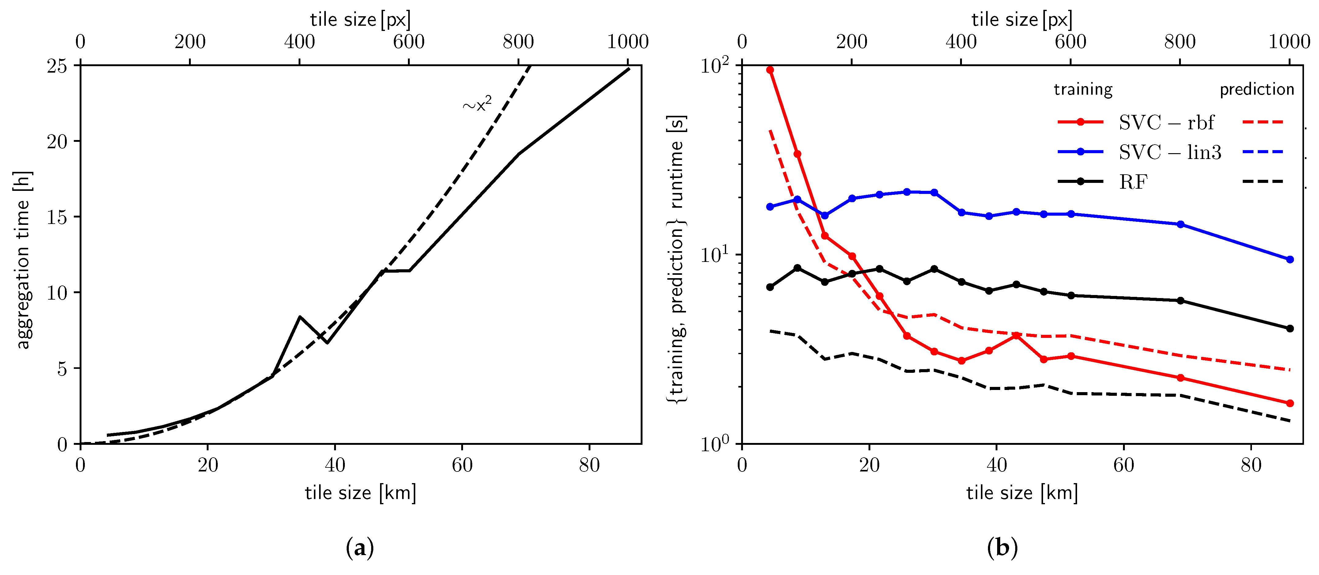
Figure 3 shows how aggregation, training, and prediction runtimes scale with tile size. By far the largest cost, aggregation (Figure 3a) takes between 1 and 25 h and scales approximately with tile size squared. This is expected, as the total number of tiles is basically constant. We note that aggregation is a perfectly parallel problem, i.e., parallelisation should result in a linear speed-up. However, we did not attempt parallelisation of the process in this project.
Training (solid lines in Figure 3b) is orders of magnitudes faster, typically taking seconds to minutes depending on the ML algorithm. As the size of the feature matrix is largely independent of tile size, the same should be true of training runtime, which is indeed the case for RF-100 and SVC-LIN. For SVC-RBF, however, training runtime varies significantly, from 1.6 s at to 95 s at , which may be due to the large overlap and hence rather strongly correlated training samples at large tile sizes.
Finally, prediction runtime (dashed lines in Figure 3b) generally follows the same trends: it is largely independent of tile size for RF-100 and SVC-LIN, but it is strongly dependent on tile size for SVC-RBF. Prediction is about as fast as training for SVC-RBF, and about four times faster for RF-100. For SVC-LIN, prediction is 100 times faster than training, takes less than 0.05 s, and was omitted from Figure 3b for clarity.
Memory usage varied between 1.8 and 2.2 GB. A larger workstation or cluster implementation should be sufficient to run the algorithm for the entire continent of Australia.
2.5. Hyperparameter Tuning
Classification accuracy and runtime performance depend on the choice of hyperparameters: parameters specific to the ML algorithm, which are selected before training, and should be tuned for the problem at hand.
For the support vector machines, there are two hyperparameters: a regularization parameter C and a kernel coefficient [45]. Since training is rapid in our case, we conducted a simple grid search, which produced an optimum and for SVC-RBF, and for SVC-LIN.
For the random forest classifier, one has to specify the number of decision trees. We report results for a random forest consisting of 100 decision trees (RF-100). We have also tested RF-1000, which increased training and prediction time by a factor of 10 (as expected), improved accuracy by merely 0.2%, and produced virtually identical maps.
3. Results
We visualise results by generating maps such as those in Figure 4. Semitransparent colours indicate the predicted landclass, dashed lines indicate training regions, and both are overlaid on top of the flatness map. A square (or circle) in the bottom right corner indicates the tile size. As explained above, tiles from the training set (i.e., those within dashed lines) may still be misclassified, which is the case if post-training accuracy is less than 100%.
3.1. Effect of Tile Size on Accuracy
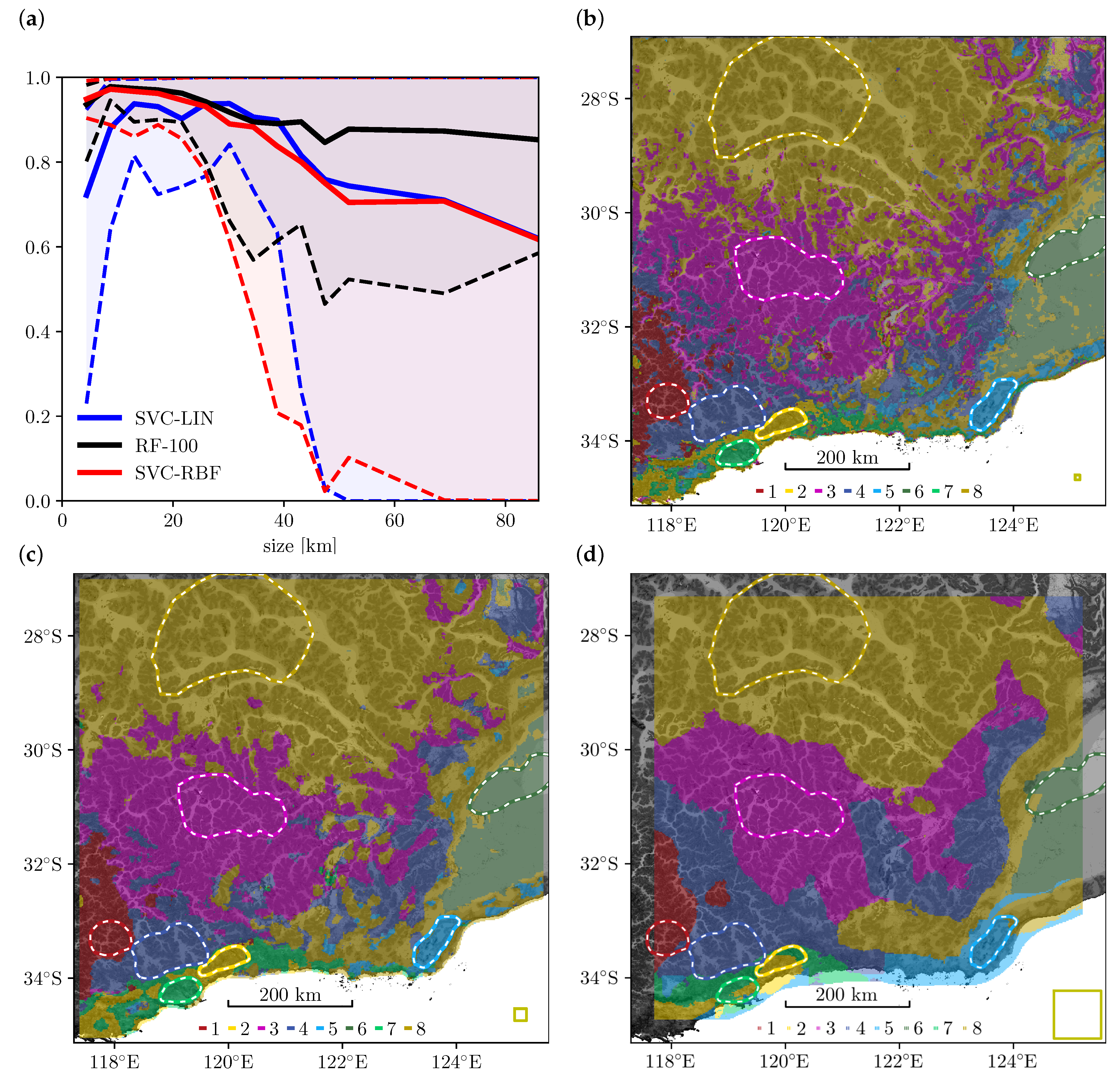
In this section, we will discuss the effect of tile size on the classification accuracy for different models. As expected, this effect is quite significant: “All spatial analyses are sensitive to the length, area, or volume over which a variable is distributed in space” [55]. In Figure 4a, we varied tile size from 4.4 to 86 km (51 to 1001 px), which produced an accuracy between and , shown by solid lines, for each of our models. Shaded areas indicate the range of per-class accuracy, again per-model, which we will discuss further below.
On average, RF-100 (black line) produces the highest accuracy, followed by SVC-LIN (blue) and SVC-RBF (red). The best map, shown in panel (b), had an accuracy of 97.8% and was produced by RF-100 with a tile size of 8.7 km (101 px). This was the second smallest tile size we tested. The minimum per-class accuracy in this case was 94.6%, indicating excellent classification for every landclass.
The remaining algorithms achieve best accuracy at similarly small tile sizes. Accuracy peaks at for SVC-RBF, and for SVC-LIN. The resulting maps, shown in Figure 5, are not fundamentally different from the overall best map in Figure 4b.
In general, smaller tiles increase the (nominal) map resolution and the number of available training samples, too little of which typically degrade accuracy. However, smaller tiles also increase the time required for aggregation and training. More severely, smaller tiles may no longer capture the spatial scales which define a particular landscape. The result is a noisy map. Conversely, larger tiles reduce noise and generate smoother boundaries between classes: Figure 4c shows a map with a tile size of , which still results in 96.3% accuracy. However, larger tiles also reduce the number of available training samples, possibly to zero for small training regions.
Overlapping tiles, i.e., partly reusing data, may alleviate this problem, at the risk of producing overfitted models that fail to generalise well. This can be observed in Figure 4d, for landclass 7: the training region is smaller than the tile size, which means that without overlap, there would be no training samples at all. With a constant stride size, the overlap is 97.5% and produces 519 training samples. Yet, accuracy for this class is only 33%, due to the lack of independent training samples. In general, classes with small training regions yield the lowest class accuracy (i.e., classes 2, 5 and 7 in our example). In Figure 4a, the shaded region indicates the range of per-class accuracy. The maximum per-class accuracy is always close to 100% i.e., there is always a class that is almost perfectly predicted. The minimum per-class accuracy, however, decreases for tile sizes larger than 30 km, quite dramatically so for the support vector models (red and blue dashed lines), and slightly less severely for RF-100 (black). It is this misclassification of small training classes that reduces overall accuracy as tiles get larger; we remind the reader that we define overall accuracy as the mean of post-training class accuracy.
3.2. Feature Importance
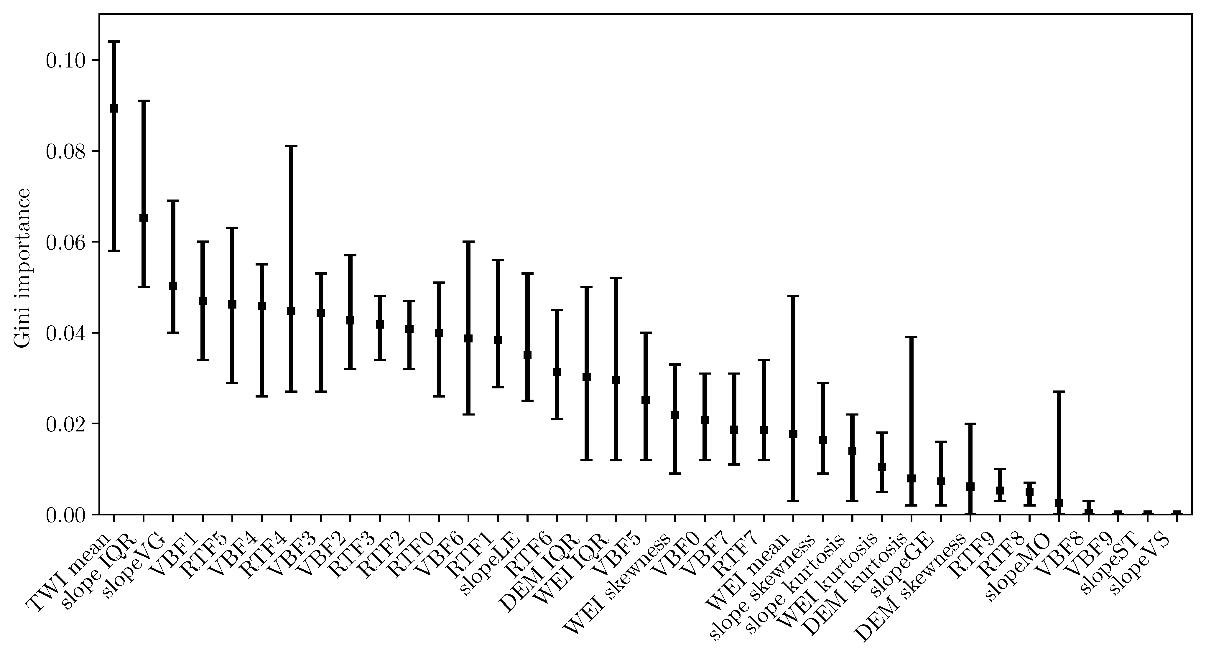
Figure 6 shows the Gini importance for the 37 features, averaged over all runs of different tile size and overlap, as discussed in Section 3.1. Squares denote the mean importance, while error bars show minimum and maximum importance. While there is some variation, the overall trend is confirmed: features that are important on average generally remain so irrespective of resolution and tile size. The most important features are topographic wetness index, slope IQR, and slopeVG, with the first two being significantly more important that the rest. Importance for subsequent features decreases approximately linear. The vast majority of features does indeed contribute to the model. Least important ones (VBF9, slopeST, slopeVS) are so because there are few tiles with these values.
3.3. Circular Tiles
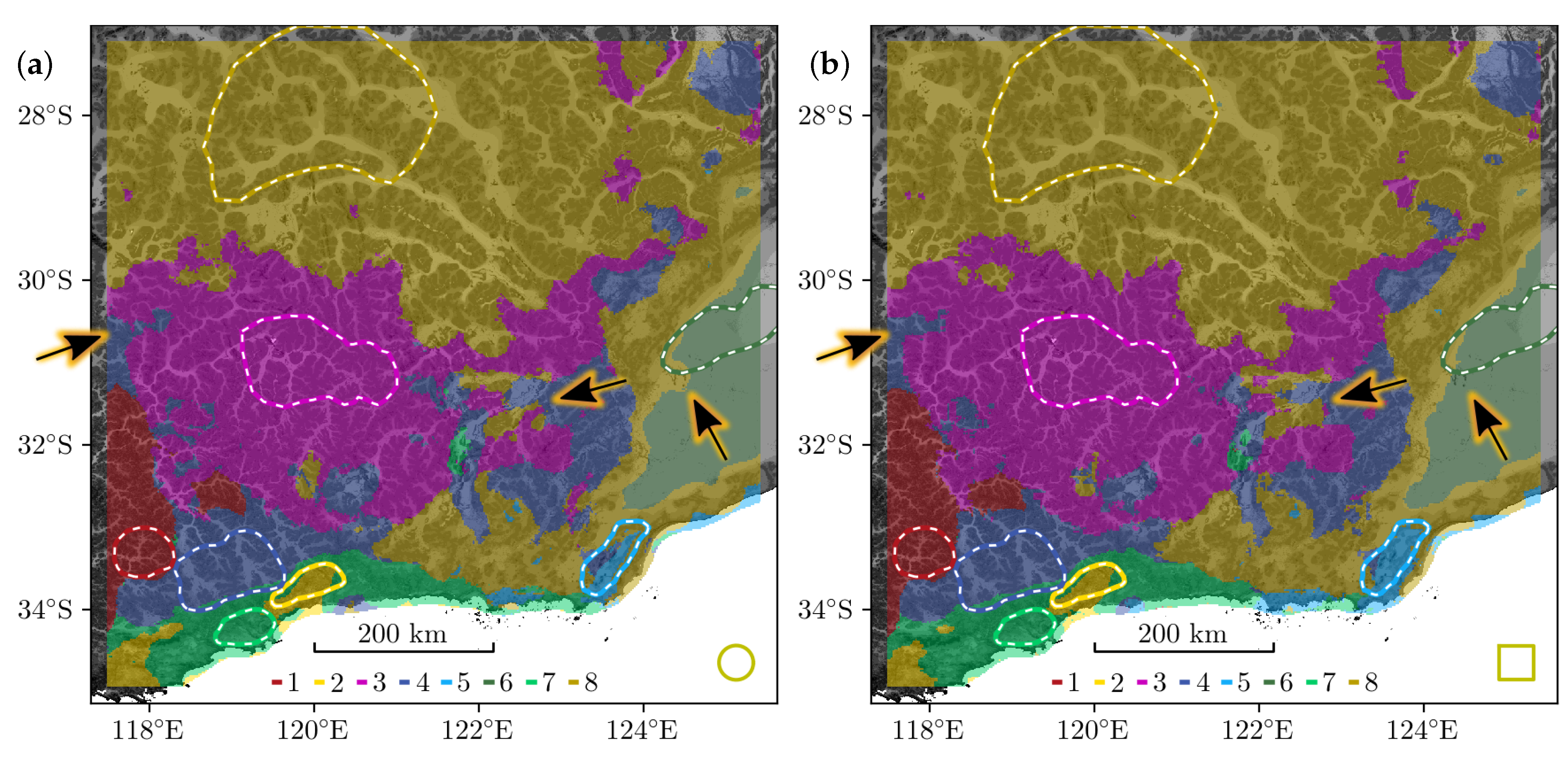
Square tiles are easy to implement, but they come with two issues. First, the resulting classification is not rotationally invariant; rotating the source data changes which part of said data gets aggregated in a particular tile (unless we rotate by multiples of 90 degrees). Consequently, the predicted map changes, which is generally unwanted. Second, square tiles tend to produce blocky shapes, which becomes most apparent for large block sizes, and especially for RF-100. Circular tiles can alleviate both issues. We also found they improve accuracy slightly (by ), at the expense of a similar increase in aggregation time. Arrows in Figure 7 highlight some rather subtle differences between square and circular tiles for RF-100 at .
3.4. Transition Belts
Landscapes vary in morphology based on different climatic conditions, basement architecture and lithologies, tectonic activity, and sedimentary dynamic regimes. All of these factors have a large footprint. Major changes in any of these variables result in changes in morphology. Often gradual in nature, we refer to these changes as transition belts. Sharp boundaries, however, may be geologically important, as they may indicate a sudden change in underlying geological structures, lithological packages, or a sharp change in the sedimentary dynamic driving forces (e.g., sedimentary river dominated regions versus transgression–regression-dominated regions; Figure 1; (e.g., [11])).
However, so far, we have posed the landscape classification problem as binary; a tile belongs to one and only one class. By definition, this leads to a sharp boundary between any two classes. This section describes a feature that implements transition belts.
Of mostly cosmetic value is a purely geometric approach, in which one may define a belt of fixed width (e.g., 20 km) along class boundaries. Support vector machines and random forests allow for more advanced approaches, each providing suitable but slightly different measures.
Support vector machines provide for every sample a distance to the decision boundary. Note that this is a distance in feature space, entirely unrelated to a distance on the map. This distance could be considered a proxy for the probability that a sample belongs to a class; a sample immediately upon a decision boundary is equally likely to belong to either class. Since our features are normalised, we could choose a threshold distance beyond which a sample is considered to belong to a particular class with 100% certainty. Below that threshold, we could linearly interpolate the probability.
Random forests report for every class a probability that a given sample belongs to that class. The probability is simply the portion of decision trees in the random forest that predict said class for the sample in question.
The results of implementing this idea are shown in Figure 8. Transparency represents probability or uncertainty, with opaque areas corresponding to a high probability (>80%) that a given sample belongs to the class indicated by the colour. Therefore, mostly translucent areas indicate a slow, gradual transition from one class to another and appear as rather wide belts between classes. Conversely, a narrow transition belt indicates a distinct, sharp class boundary. This is purely a postprocessing feature and comes with no significant computational costs.
3.5. Novelty Detection
Located in the SW of our model region, the Stirling Range is distinct from its surroundings, rising to m above sea level in an otherwise largely flat area. A domain expert would clearly identify it as a separate class. However, we have ommitted the Stirling Range from our classification so far, as its rather small spatial extent provides few training samples at our 3-arc-sec DEM resolution. For the same reason, we have omitted coastal regions, which are distinct from the inland patterns due to the modern sedimentary dynamics of the coast (e.g., erosional regime of incident waves, coastline, and mobile sand dune systems).
It would be useful if our algorithm detected such instances, i.e., those which do not resemble any training data. Known as outlier or novelty detection, a number of algorithms exists for this task, of which we have tested OneClassSVM, IsolationForests, and LocalOutlierFactor. Technically, we combine training data of all classes into a single class and train a model. We then predict whether a new sample belongs to that single class (inlier) or not (outlier/novelty). Impementation is straightforward and the required additional training is cheap.
Example results are shown in Figure 9. In panel (a), the IsolationForest classifier clearly identifies as unknown (i) the Stirling Range, (ii) a similar region SW to it, and (iii) some coastal regions. Almost everything else is classified as known.
This classifier detects the Stirling Range at all tile sizes we have tested, with smaller tile sizes generally resulting in more detailed shapes which better match the boundary drawn by the domain expert. OneClassSVM (not shown) performs about the same up to , beyond which results degrade. LocalOutlierFactor (Figure 9b) produces too many false positives to be useful at all tile sizes we have tested.
4. Discussion and Conclusions
One of the most challenging aspects of landscape study is cataloguing their differences at a regional scale (e.g., [29]). The difficulty is not related to classifying the features that can differentiate landscapes into different domains, but in determining the geographic extent of such features. Field observations have been relied upon as a proxy to understand landscape diversity at a regional scale [11]. However, a constraint on this approach is the uncertainty in the extrapolation of field observations, especially when attempting to extrapolate them to regional scales. Such extrapolation suffers due to the complexity and variability of landforms, the paucity of data availability, and the difficulty in defining quantitative criteria that discriminates diverse landscape types from each other. However, there are a wide variety of existing quantitative methods in geomorphology developed for small scales (10 km). Modern data analytics technology, and the advances in satellite imaging, provides access to large data sets that can assist in characterising landscape features and their distribution at regional scales (e.g., [27,31,32,33,40]).
In this study, we have presented an automatic landscape mapping methodology. For every landclass present in the test region, a domain expert defines a sample region. After training on these sample regions, machine learning algorithms are able to predict a dense map. We tested our Python implementation using data derived from a 3-arc-second digital elevation model for a region in Western Australia of approximately . At an optimised tile size, we achieve an accuracy of almost 98%, with a reasonable runtime of 48 min.
Spatial aggregation of the raw pixel values is crucial to classification accuracy, but it is crucial in a way that conserves some spatial variation. We found a per-tile normalised histogram approach to work well. Classification based on raw pixel values fared much worse, which is consistent with the observation that performance of the normalised histogram approach degrades as the tile size approaches zero (see Figure 4). While currently the most expensive computationally, this aggregation stage could see a significant speedup through advanced vectorisation, or possibly a C++ implementation.
We also presented three extensions: (i) circular tiles, which enable rotationally invariant classification, (ii) transition belts, which indicate how gradual or abrupt landscapes change, and (iii) novelty detection, which can identify regions which do not match any of the landclasses defined during training.
The methodology presented is a building block of a future toolbox that will allow landscape types to be mapped at continental scale using remote sensing techniques and machine learning algorithms. Our approach is scalable and repeatable, both spatially and temporally. We note, however, that ML does not necessarily remove subjectivity. Results still depend on which and how many polygons the domain expert chooses for training, and the size and stride of tiles. Larger tiles produce a more contiguous but lower resolution map. Conversely, smaller tiles result in a more detailed, and at some point, noisy map. The choice of ML algorithm is not overly critical: random forest and support vector machine classifiers generate quite similar maps, which is a favourable outcome.
This work builds on previous studies about characterisation of landscapes in the South of Western Australia and worldwide (e.g., [5,18,29], and references therein). The diversity and distribution of landscapes mapped in this study support previous results presented by domain experts, which were based on field observations [11]. This study identified four main landscape domains in several field regional transects, conducted at different latitudes in the South of Western Australia (Figure 1). These transects were designed to capture the geomorphological variability between typical landscape features in the Yilgarn Craton to the coastline, in order to characterize the landscape evolution.
The landscape changes were summarised from the topographically high, dissected environment with thick cover development and uneven basement topography, to the nearly flat coastal regions with thin cover and sand dune systems at the coastline. These differential landscape domains were identified in a previous study and classified into a framework of four different landscape types: (i) Albany (green, Figure 9); (ii) Kalgoorlie–Norseman (pink and dark blue); (iii) Esperance (bright blue and dark green); and (iv) Neale (dark yellow) [9].
Gonzalez-Alvarez et al. [11] faced three main challenges after reconstructing the transects and the observations from the field: (i) how to infer their direct observations along the traverses laterally, (ii) how to clearly identify boundaries between landscape types along the traverses, and (iii) how to profile the landscape types with specific features or combination of features. The present study identifies the four landscape domains mentioned above, which substantiates the methodology. It also addresses all three of the above challenges. In addition, our results are geologically meaningful since they are consistent with the geological trends and main basement features in the region. The extension and boundaries of the landscape types defined are an important contribution to the understanding of landscape evolution of this region in Western Australia. Landscape variability is directly related to sedimentary regimes. Sedimentary regimes dominated by erosional processes may provide the best context to detect the geochemical footprint of ore bodies located at depth. In contrast, depositional regimes may obscure that geochemical signature by bringing exotic material to the region. The stratigraphic variability of the cover captures landscape evolution, and, therefore, links the geology at depth with the surface. Mapping landscape variability allows for a better understanding of the relation between sedimentary regimes, landscape evolution, and geology. Therefore, landscape mapping can be used as a valuable tool in mineral exploration.
In the context of mineral exploration in intensely weathered regions of low relief, our results support that DEM can be used to (i) discriminate and characterise landscape variability types at large scales, (ii) map the extension of the landscape domains, (iii) quantify their surface geometrical features, and (iv) establish the transitional boundaries between landscapes. These outputs offer valuable assistance in the design and interpretation of surface geochemical surveys at a regional scale in areas of low relief and intensely weathered landscapes. The variability of the landscape types can reflect geological, tectonic, and stratigraphic changes. Identifying such changes can be fundamental for a more efficient interpretation of surface geochemical data (e.g., detecting the geochemical footprint of potential ore deposits at depth, establishing changes in surface biodiversity associated to geological changes at depth, detecting diverse tectonic regimes, etc.).
Author Contributions
Methodology, software, validation, formal analysis, investigation, data curation, writing—original draft preparation, and visualisation, Thomas Albrecht; conceptualisation, writing—review and editing, project administration, and funding acquisition, Ignacio González-Álvarez and Jens Klump. All authors have read and agreed to the published version of the manuscript.
Funding
Support by the Discovery Program through its strategic funding (CSIRO, Mineral Resources) is gratefully acknowleged.
Data Availability Statement
Publicly available datasets were analyzed in this study, summarised and referenced in Table 1.
Acknowledgments
We would like to thank Greg Smith for his insights and work when the project started, Tania Ibrahimi for her assistance with GIS and the preparation of some of the figures, and Tim Prokopiuk for his insights. We thank three anonymous reviewers for their constructive advice that greatly improved this manuscript and thank the managing editor Rocksy Zhang for her assistance handling this paper. Support by the Discovery Program through its strategic funding (CSIRO, Mineral Resources) is gratefully acknowleged.
Conflicts of Interest
The authors declare no conflict of interest. The funders had no role in the design of the study; in the collection, analyses, or interpretation of data; in the writing of the manuscript; or in the decision to publish the results.
Abbreviations
The following abbreviations are used in this manuscript:
| DEM | Digital elevation model |
| ML | Machine learning |
| RF-100 | Random forest consisting of 100 decision trees |
| SRTM | Shuttle Radar Topography Mission |
| SVC-LIN | Support vector machine classifier with linear kernel |
| SVC-RBF | Support vector machine classifier with radial basis function kernel |
References
- González-Álvarez, I.; Goncalves, M.; Carranza, J. Introduction to the Special Issue- Challenges for Mineral Exploration in the 21st Century: Targeting Mineral Deposits Undercover. Ore Geol. Rev. Spec. Issue 2020, 126, 103785. [Google Scholar] [CrossRef]
- Butt, C.R.M.; Lintern, M.; Anand, R.R. Evolution of regoliths and landscapes in deeply weathered terrain—Implications for geochemical exploration. Ore Geol. Rev. 2000, 16, 167–183. [Google Scholar] [CrossRef]
- Butt, C.; Robertson, I.; Scott, K.; Cornelius, M. Regolith expression of Australian ore systems: A compilation of exploration case histories with conceptual dispersion, process and exploration models; CRC LEME: Perth, WA, Australia, 2005. [Google Scholar]
- Anand, R.R. Importance of 3-D regolith-landform control in areas of transported cover: Implications for geochemical exploration. Geochem. Explor. Environ. Anal. 2016, 16, 14–26. [Google Scholar] [CrossRef]
- Goudie, A. Encyclopedia of Eomorphology; Psychology Press: London, UK, 2004. [Google Scholar]
- González-Álvarez, I.; Boni, M.; Anand, R.R. Mineral exploration in regolith-dominated terrains: Global considerations and challenges. Ore Geol. Rev. 2016, 73, 375–379. [Google Scholar] [CrossRef]
- Anand, R.R.; Butt, C.R.M. A guide for mineral exploration through the regolith in the Yilgarn Craton, Western Australia. Aust. J. Earth Sci. 2010, 57, 1015–1114. [Google Scholar] [CrossRef]
- Smith, R.E.; Perdrix, J.; Davis, J. Dispersion into pisolitic laterite from the Greenbushes mineralized Sn-Ta pegmatite system, Western Australia. J. Geochem. Explor. 1987, 28, 251–265. [Google Scholar] [CrossRef]
- Xueqiu, W.; Bimin, Z.; Xin, L.; Shanfa, X.; Wensheng, Y.; Rong, Y. Geochemical challenges of diverse regolith-covered terrains for mineral exploration in China. Ore Geol. Rev. 2016, 73, 417–431. [Google Scholar] [CrossRef]
- Chen, X.; Lintern, M.; Roach, I. Calcrete: Characteristics, Distribution and Use in Mineral Exploration. CRC LEME, Cooperative Research Centre for Landscape Environments and Mineral Exploration; Technical Report; CSIRO Exploration and Mining: Perth, WA, Australia, 2002. [Google Scholar]
- González-Álvarez, I.; Salama, W.; Anand, R.R. Sea-level changes and buried islands in a complex coastal palaeolandscape in the South of Western Australia: Implications for greenfield mineral exploration. Ore Geol. Rev. 2016, 73, 475–499. [Google Scholar] [CrossRef]
- Chardon, D.; Grimaud, J.L.; Beauvais, A.; Bamba, O. West African lateritic pediments: Landform-regolith evolution processes and mineral exploration pitfalls. Earth Sci. Rev. 2018, 179, 124–146. [Google Scholar] [CrossRef]
- Winterburn, P.A.; Noble, R.R.; Lawie, D. Advances in exploration geochemistry, 2007 to 2017 and beyond. Geochem. Explor. Environ. Anal. 2020, 20, 157–166. [Google Scholar] [CrossRef] [Green Version]
- Anand, R.; Hough, R.; Salama, W.; Aspandiar, M.; Butt, C.; González-Álvarez, I.; Metelka, V. Gold and pathfinder elements in ferricrete gold deposits of the Yilgarn Craton of Western Australia: A review with new concepts. Ore Geol. Rev. 2019, 104, 294–355. [Google Scholar] [CrossRef]
- González-Álvarez, I.; Salama, W.; Hilliard, P.; Ibrahimi, T.; LeGras, M.; Rondon-Gonzalez, O. Landscape evolution and geochemical dispersion of the DeGrussa Cu-Au deposit, Western Australia. Ore Geol. Rev. 2019, 105, 487–513. [Google Scholar] [CrossRef]
- Summerfield, M.A. Neotectonics and landform genesis. Prog. Phys. Geogr. 1987, 11, 384–397. [Google Scholar] [CrossRef]
- Ollier, C.D. Evolution of the Australian landscape. Mar. Freshw. Res. 2001, 52, 13–23. [Google Scholar] [CrossRef]
- Twidale, C.R. Ancient Australian Landscapes; Rosenberg Publishing: Dural, NSW, Australia, 2007. [Google Scholar]
- Pain, C.F.; Pillans, B.J.; Roach, I.C.; Worrall, L.; Wilford, J.R. Shaping a Nation: A Geology of Australia; Chapter Old, Flat and Red–Australia’s Distinctive Landscape; ANU Press: Canberra, ACT, Australia, 2012; pp. 227–276. [Google Scholar] [CrossRef] [Green Version]
- Egletton, R.A. (Ed.) The Regolith Glossary: Surficial Geology, Soils and Landscapes; CRC LEME: Perth, WA, Australia, 2001. [Google Scholar]
- Otto, J.C.; Prasicek, G.; Blöthe, J.; Schrott, L. GIS Applications in Geomorphology. In Comprehensive Geographic Information Systems; Huang, B., Ed.; Elsevier: Oxford, UK, 2018; pp. 81–111. [Google Scholar] [CrossRef]
- Costanza, J.K.; Riitters, K.; Vogt, P.; Wickham, J. Describing and analyzing landscape patterns: Where are we now, and where are we going? Landsc. Ecol 2019, 34, 2049–2055. [Google Scholar] [CrossRef] [Green Version]
- Gustafson, E.J. How has the state-of-the-art for quantification of landscape pattern advanced in the twenty-first century? Landsc. Ecol. 2019, 34, 2065–2072. [Google Scholar] [CrossRef]
- Frazier, A.E.; Kedron, P. Landscape metrics: Past progress and future directions. Curr. Landsc. Ecol. Rep. 2017, 2, 63–72. [Google Scholar] [CrossRef] [Green Version]
- Lausch, A.; Blaschke, T.; Haase, D.; Herzog, F.; Syrbe, R.U.; Tischendorf, L.; Walz, U. Understanding and quantifying landscape structure–A review on relevant process characteristics, data models and landscape metrics. Ecol. Model. 2015, 295, 31–41. [Google Scholar] [CrossRef]
- Jasiewicz, J.; Niesterowicz, J.; Stepinski, T. Multi-resolution, pattern-based segmentation of very large raster datasets. In Proceedings of the International Conference on GIScience, Montreal, QC, Canada, 27–30 September 2016; Volume 1. [Google Scholar]
- Jasiewicz, J.; Netzel, P.; Stepinski, T.F. Landscape similarity, retrieval, and machine mapping of physiographic units. Geomorphology 2014, 221, 104–112. [Google Scholar] [CrossRef]
- Jasiewicz, J.; Stepinski, T.; Niesterowicz, J. Multi-scale segmentation algorithm for pattern-based partitioning of large categorical rasters. Comput. Geosci. 2018, 118, 122–130. [Google Scholar] [CrossRef] [Green Version]
- Ollier, C.D. Terrain classification: Methods, Applications and Principles. In Applied Geomorphology; Elsevier: Amsterdam, The Netherlands, 1978. [Google Scholar]
- Soranno, P.A.; Wagner, T.; Collins, S.M.; Lapierre, J.F.; Lottig, N.R.; Oliver, S.K. Spatial and temporal variation of ecosystem properties at macroscales. Ecol. Lett. 2019, 22, 1587–1598. [Google Scholar] [CrossRef]
- Wilford, J.R.; Searle, R.; Thomas, M.; Pagendam, D.; Grundy, M.J. A regolith depth map of the Australian continent. Geoderma 2016, 266, 1–13. [Google Scholar] [CrossRef]
- de Caritat, P.; Main, P.T.; Grunsky, E.C.; Mann, A.W. Recognition of geochemical footprints of mineral systems in the regolith at regional to continental scales. Aust. J. Earth Sci. 2017, 64, 1033–1043. [Google Scholar] [CrossRef] [Green Version]
- Caruso, A.; Clarke, K.; Tiddy, C.; Delean, S.; Lewis, M. Objective Regolith-Landform Mapping in a Regolith Dominated Terrain to Inform Mineral Exploration. Geosciences 2018, 8, 318. [Google Scholar] [CrossRef] [Green Version]
- Mercader, J.; Martı, R.; González, I.J.; Sánchez, A.; Garcıa, P. Archaeological site formation in rain forests: Insights from the Ituri rock shelters, Congo. J. Archaeol. Sci. 2003, 30, 45–65. [Google Scholar] [CrossRef]
- Abdi, A.M. Land cover and land use classification performance of machine learning algorithms in a boreal landscape using Sentinel-2 data. GIScience Remote Sens. 2020, 57, 1–20. [Google Scholar] [CrossRef] [Green Version]
- Zhang, Y.; Li, Q.; Huang, H.; Wu, W.; Du, X.; Wang, H. The combined use of remote sensing and social sensing data in fine-grained urban land use mapping: A case study in Beijing, China. Remote Sens. 2017, 9, 865. [Google Scholar] [CrossRef] [Green Version]
- Lidberg, W.; Nilsson, M.; Ågren, A. Using machine learning to generate high-resolution wet area maps for planning forest management: A study in a boreal forest landscape. Ambio 2020, 49, 475–486. [Google Scholar] [CrossRef] [PubMed] [Green Version]
- Maxwell, A.E.; Warner, T.A.; Fang, F. Implementation of machine-learning classification in remote sensing: An applied review. Int. J. Remote Sens. 2018, 39, 2784–2817. [Google Scholar] [CrossRef] [Green Version]
- Fouedjio, F.; Klump, J. Exploring prediction uncertainty of spatial data in geostatistical and machine learning approaches. Environ. Earth Sci. 2019, 78, 38. [Google Scholar] [CrossRef]
- Jasiewicz, J.; Netzel, P.; Stepinski, T. GeoPAT: A toolbox for pattern-based information retrieval from large geospatial databases. Comput. Geosci. 2015, 80, 62–73. [Google Scholar] [CrossRef]
- Gallant, J.C.; Wilson, N.; Dowling, T.I.; Read, A.; Inskeep, C. SRTM-Derived 3 Second Digital Elevation Models Version 1.0; Technical Report; Geoscience Australia: Canberra, ACT, Australia, 2009. [Google Scholar]
- Gallant, J.C.; Dowling, T.I. A multiresolution index of valley bottom flatness for mapping depositional areas. Water Resour. Res. 2003, 39. [Google Scholar] [CrossRef]
- Kuhn, M.; Johnson, K. Applied Predictive Modeling; Springer: New York, NY, USA, 2013. [Google Scholar] [CrossRef]
- Fan, R.E.; Chang, K.W.; Hsieh, C.J.; Wang, X.R.; Lin, C.J. LIBLINEAR: A library for large linear classification. J. Mach. Learn. Res. 2008, 9, 1871–1874. [Google Scholar]
- Chang, C.C.; Lin, C.J. LIBSVM: A Library for Support Vector Machines. ACM Trans. Intell. Syst. Technol. 2011, 2, 27:1–27:27. [Google Scholar] [CrossRef]
- Breiman, L. Classification and Regression Trees; Chapman and Hall: Boca Raton, FL, USA, 2017. [Google Scholar]
- Breiman, L. Random forests. Mach. Learn. 2001, 45, 5–32. [Google Scholar] [CrossRef] [Green Version]
- Pedregosa, F.; Varoquaux, G.; Gramfort, A.; Michel, V.; Thirion, B.; Grisel, O.; Blondel, M.; Prettenhofer, P.; Weiss, R.; Dubourg, V.; et al. Scikit-learn: Machine Learning in Python. J. Mach. Learn. Res. 2011, 12, 2825–2830. [Google Scholar]
- Gallant, J.C.; Dowling, T.I.; Austin, J. Multi-Resolution Ridge Top Flatness (MrRTF) v2; Technical Report; CSIRO: Canberra, ACT, Australia, 2013. [Google Scholar]
- Gallant, J.C.; Austin, J. Topographic Wetness Index Derived from 1" SRTM DEM-H. v2.; Technical Report; CSIRO: Canberra, ACT, Australia, 2012. [Google Scholar]
- Gallant, J.C.; Austin, J. Slope Derived from 1" SRTM DEM-S. v4; Technical Report; CSIRO: Canberra, ACT, Australia, 2012. [Google Scholar]
- Böhner, J.; Antonić, O. Land-surface parameters specific to topo-climatology. Dev. Soil Sci. 2009, 33, 195–226. [Google Scholar]
- Gerlitz, L.; Conrad, O.; Böhner, J. Large-scale atmospheric forcing and topographic modification of precipitation rates over High Asia—a neural-network-based approach. Earth Syst. Dyn. 2015, 6, 61. [Google Scholar] [CrossRef] [Green Version]
- Gallant, J.C.; Austin, J. Slope Relief Classification Derived from 1" SRTM DEM-S. v3; Technical Report; CSIRO: Canberra, ACT, Australia, 2012. [Google Scholar]
- Han, J.; Miller, H.J. Geographic Data Mining and Knowledge Discovery; CRC Press: Boca Raton, FL, USA, 2009. [Google Scholar]
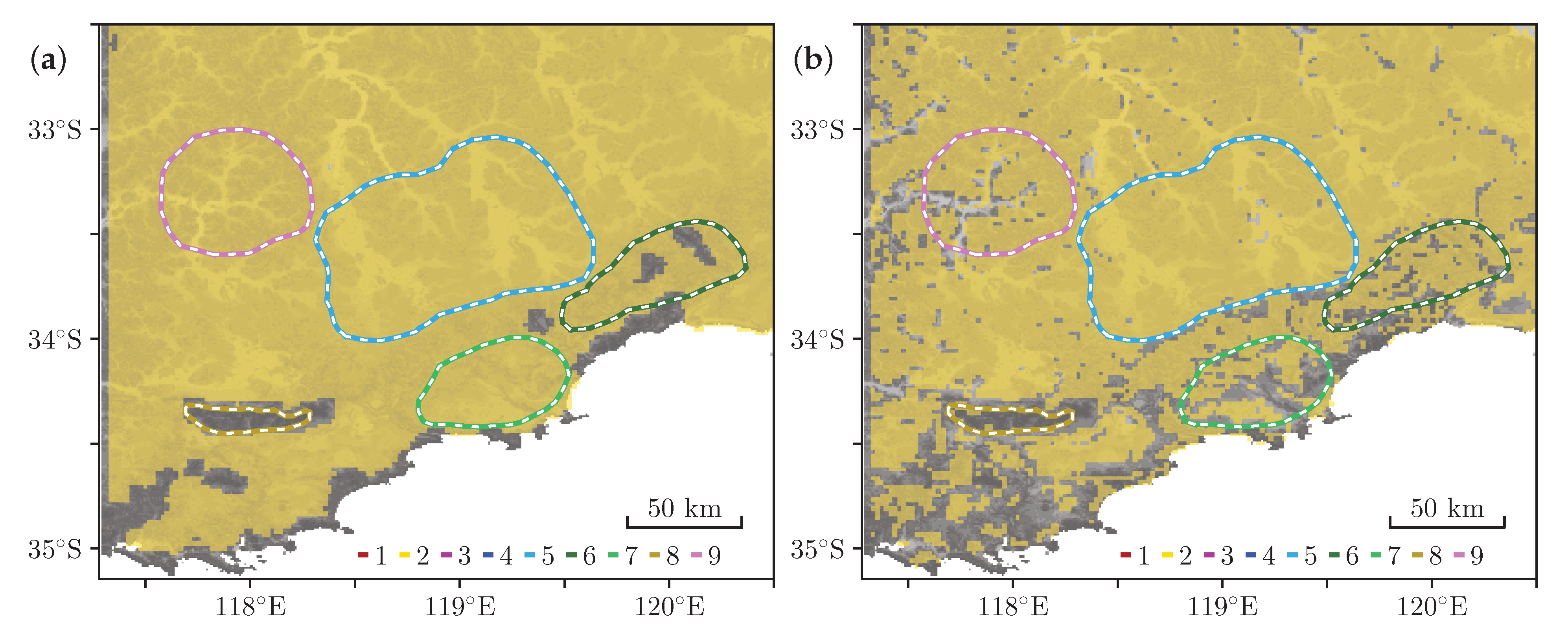
Figure 1.
(a) DEM [41] of the study area. (b) Multiresolution valley bottom flatness map (MrVBF, [42]), a subproduct of the DEM, that displays low slope gradients in lighter shade and high slope gradients in darker shade. Colour indicates the eight flatness surface patterns used in this study.

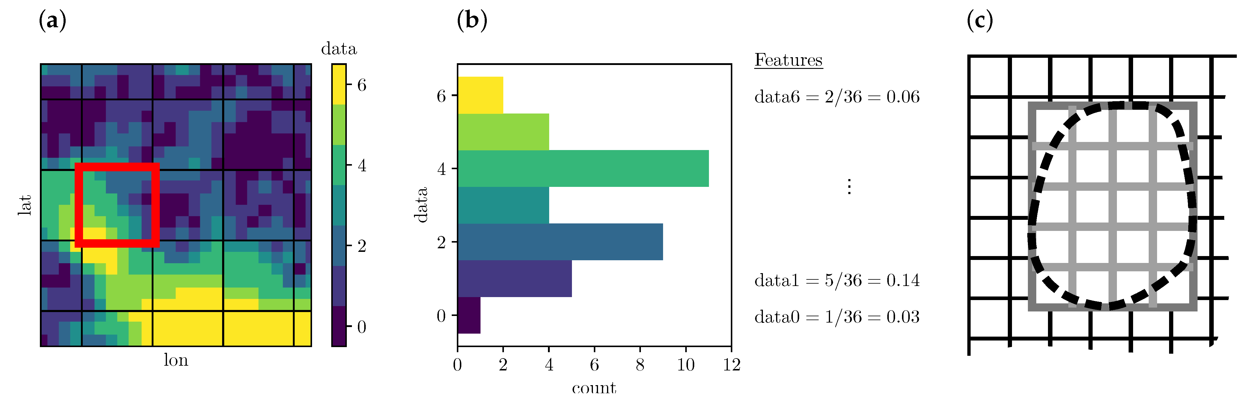
Figure 2.
Spatial feature aggregation. (a) We decompose the source data into tiles of size . (b) Within each tile, we compute the fraction of each area that is equal to a possible value. In other words, we compute per-tile normalised histograms of source data. In this example, we use and a generic field of “data” ranging 0 to 6, sorted into seven bins, which results in seven features “data0” ⋯ “data6”. (c) The bounding box of a landclass training region determines the training grid (gray), which generally differs from the grid (black) used for predicting the final map. This helps to identify overfitted models. See text for details.

Figure 3.
Effect of tile size on (a) aggregation and (b) training and prediction runtime. Note that, for clarity, we omitted prediction runtime for SVC-LIN. It has a similar (lack of) dependency on tile size as RF-100, but is two orders of magnitude faster.
Figure 3.
Effect of tile size on (a) aggregation and (b) training and prediction runtime. Note that, for clarity, we omitted prediction runtime for SVC-LIN. It has a similar (lack of) dependency on tile size as RF-100, but is two orders of magnitude faster.

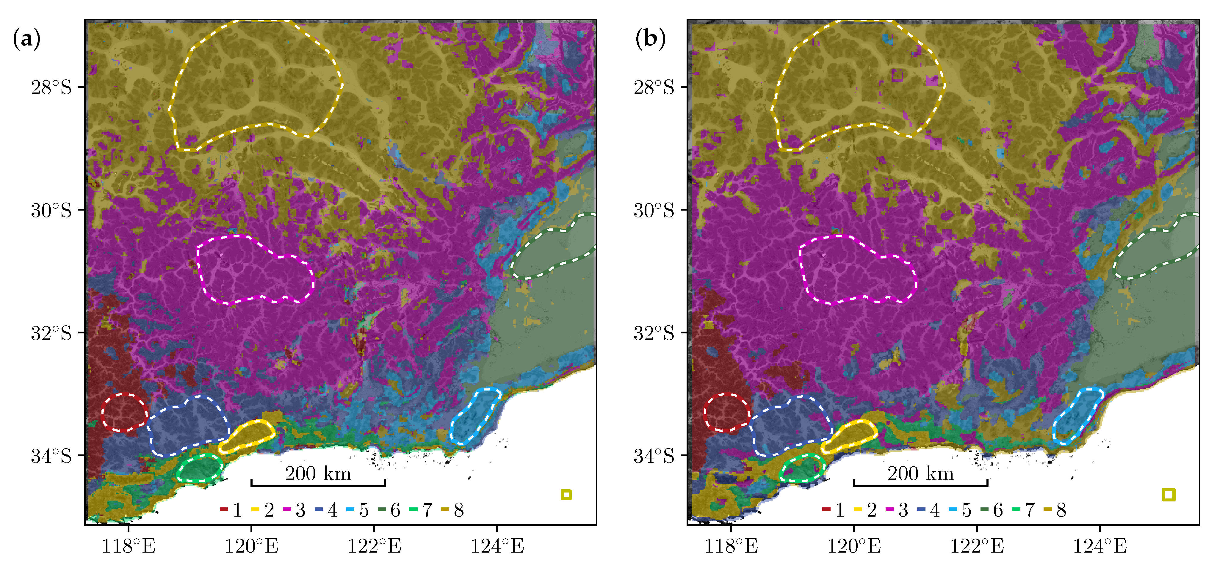
Figure 4.
(a) Solid lines show the overall accuracy vs. block size, per ML algorithm. Shaded areas indicate the range of per-class accuracy. (b) The highest accuracy score of 97.8% is produced by RF-100 at , which is still a rather small tile size and results in a somewhat noisy map. The yellow square in the lower right corner represents a tile. (c) Increasing the tile size to reduces accuracy slightly to 96.3% but produces a much cleaner map. (d) At the largest , a lack of training samples severly degrades accuracy for classes 2 and 7 whose training regions are small.

Figure 5.
Best maps as produced by the remaining classifiers: (a) SVC-RBF at , (b) SVC-LIN at .

Figure 6.
Gini importance for the 37 features (see Table 1 and Table 2). Squares denote the mean importance, while errorbars show minimum and maximum importance for runs of different tile size and overlap.

Figure 7.
Circular tiles (a) tend to result in less blocky shapes, and slightly improve detail over rectangular tiles (b). Markers indicate some of the generally subtle differences. RF-100 at .
Figure 7.
Circular tiles (a) tend to result in less blocky shapes, and slightly improve detail over rectangular tiles (b). Markers indicate some of the generally subtle differences. RF-100 at .

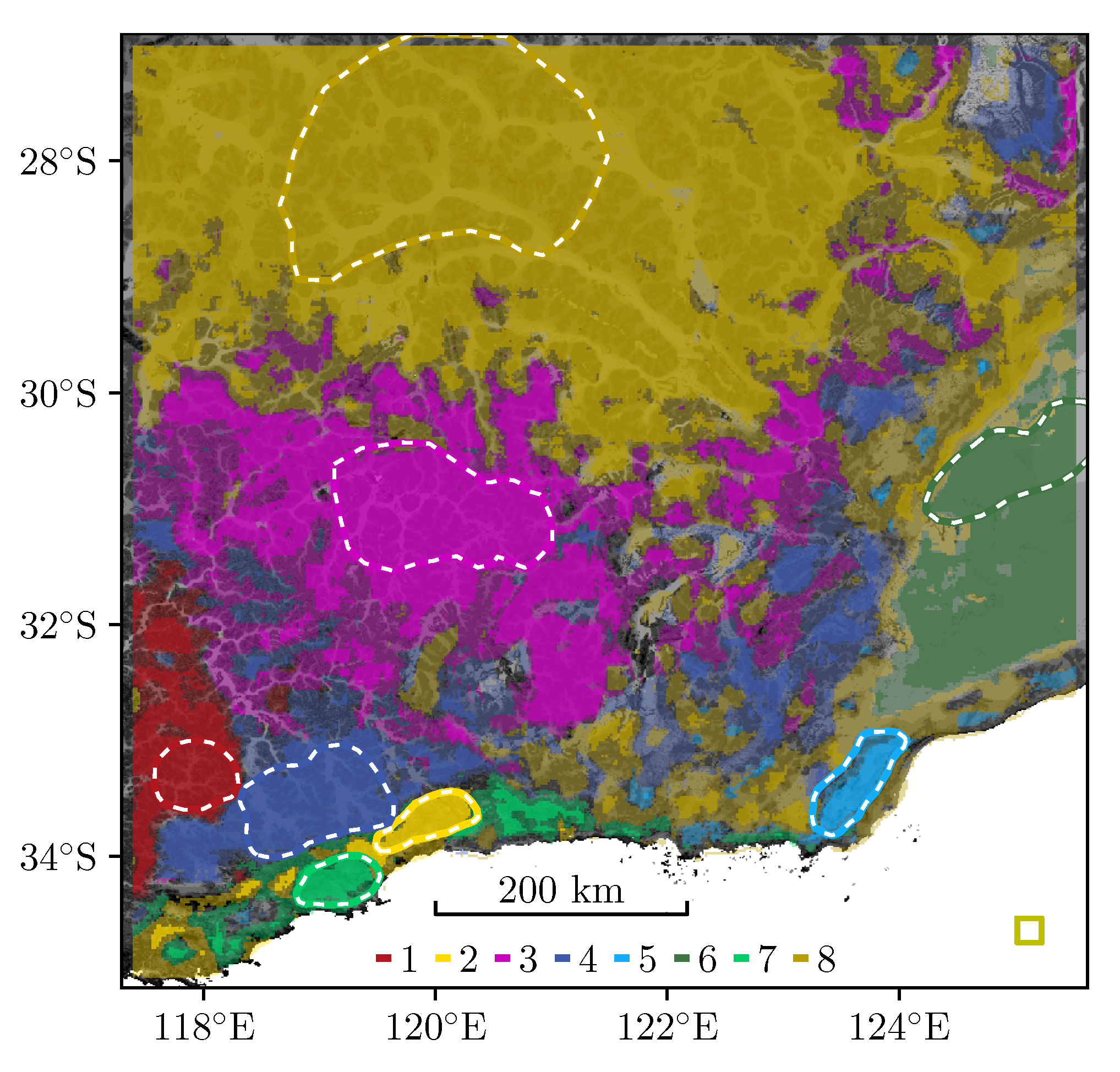
Figure 8.
Map with transition belts, RF-100 at . Clear, semiopaque, and mostly opaque areas denote <, 40–, and > probability, respectively, that a given tile belongs to the indicated class.
Figure 8.
Map with transition belts, RF-100 at . Clear, semiopaque, and mostly opaque areas denote <, 40–, and > probability, respectively, that a given tile belongs to the indicated class.

Figure 9.
Novelty detection, zoom of the SW of our model region. (a) IsolationForest, . The detected region matches the Stirling Range as marked by a human domain expert. LocalOutlierFactor (b) produces many false positives.
Figure 9.
Novelty detection, zoom of the SW of our model region. (a) IsolationForest, . The detected region matches the Stirling Range as marked by a human domain expert. LocalOutlierFactor (b) produces many false positives.

Table 3.
The number of training samples for our test region is roughly balanced.
| Class Label | 1 | 2 | 3 | 4 | 5 | 6 | 7 | 8 |
|---|---|---|---|---|---|---|---|---|
| number of training samples | 831 | 583 | 3670 | 2036 | 871 | 1869 | 560 | 9940 |
Publisher’s Note: MDPI stays neutral with regard to jurisdictional claims in published maps and institutional affiliations. |
© 2021 by the authors. Licensee MDPI, Basel, Switzerland. This article is an open access article distributed under the terms and conditions of the Creative Commons Attribution (CC BY) license (https://creativecommons.org/licenses/by/4.0/).
Share and Cite
MDPI and ACS Style
Albrecht, T.; González-Álvarez, I.; Klump, J. Using Machine Learning to Map Western Australian Landscapes for Mineral Exploration. ISPRS Int. J. Geo-Inf. 2021, 10, 459. https://doi.org/10.3390/ijgi10070459
AMA Style
Albrecht T, González-Álvarez I, Klump J. Using Machine Learning to Map Western Australian Landscapes for Mineral Exploration. ISPRS International Journal of Geo-Information. 2021; 10(7):459. https://doi.org/10.3390/ijgi10070459
Chicago/Turabian StyleAlbrecht, Thomas, Ignacio González-Álvarez, and Jens Klump. 2021. "Using Machine Learning to Map Western Australian Landscapes for Mineral Exploration" ISPRS International Journal of Geo-Information 10, no. 7: 459. https://doi.org/10.3390/ijgi10070459
Note that from the first issue of 2016, this journal uses article numbers instead of page numbers. See further details here.