
Geoinformation Technologies in Support of Environmental Hazards Monitoring under Climate Change: An Extensive Review

 ,
,  ,
,  , ,
, ,  ,
,  , ,
, , 
Abstract
:1. Introduction
Specificity of the Review Methodology of This Paper
2. Environmental Monitoring
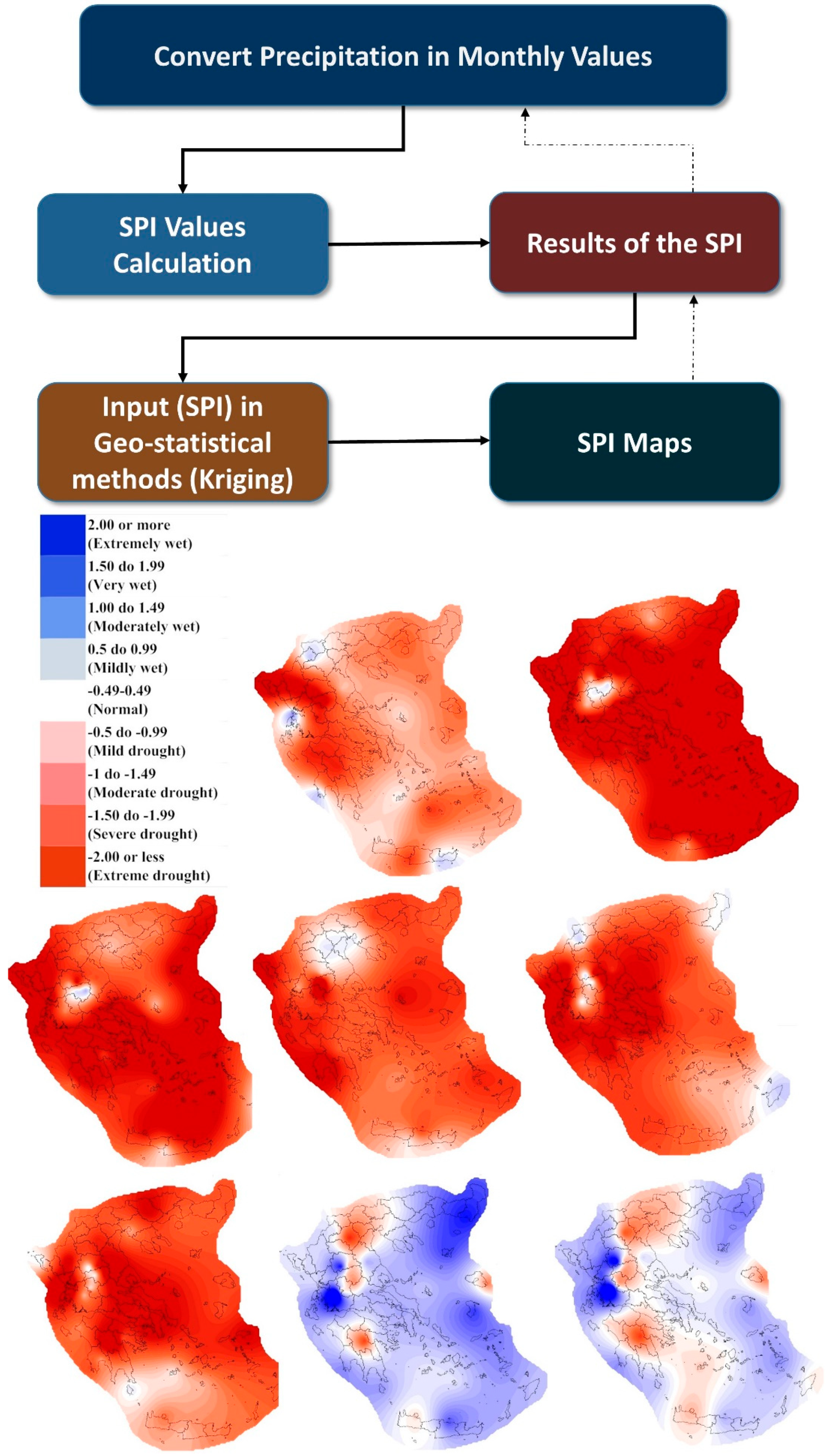
2.1. Drought Monitoring
2.2. Soil Erosion Monitoring
2.3. Groundwater Monitoring
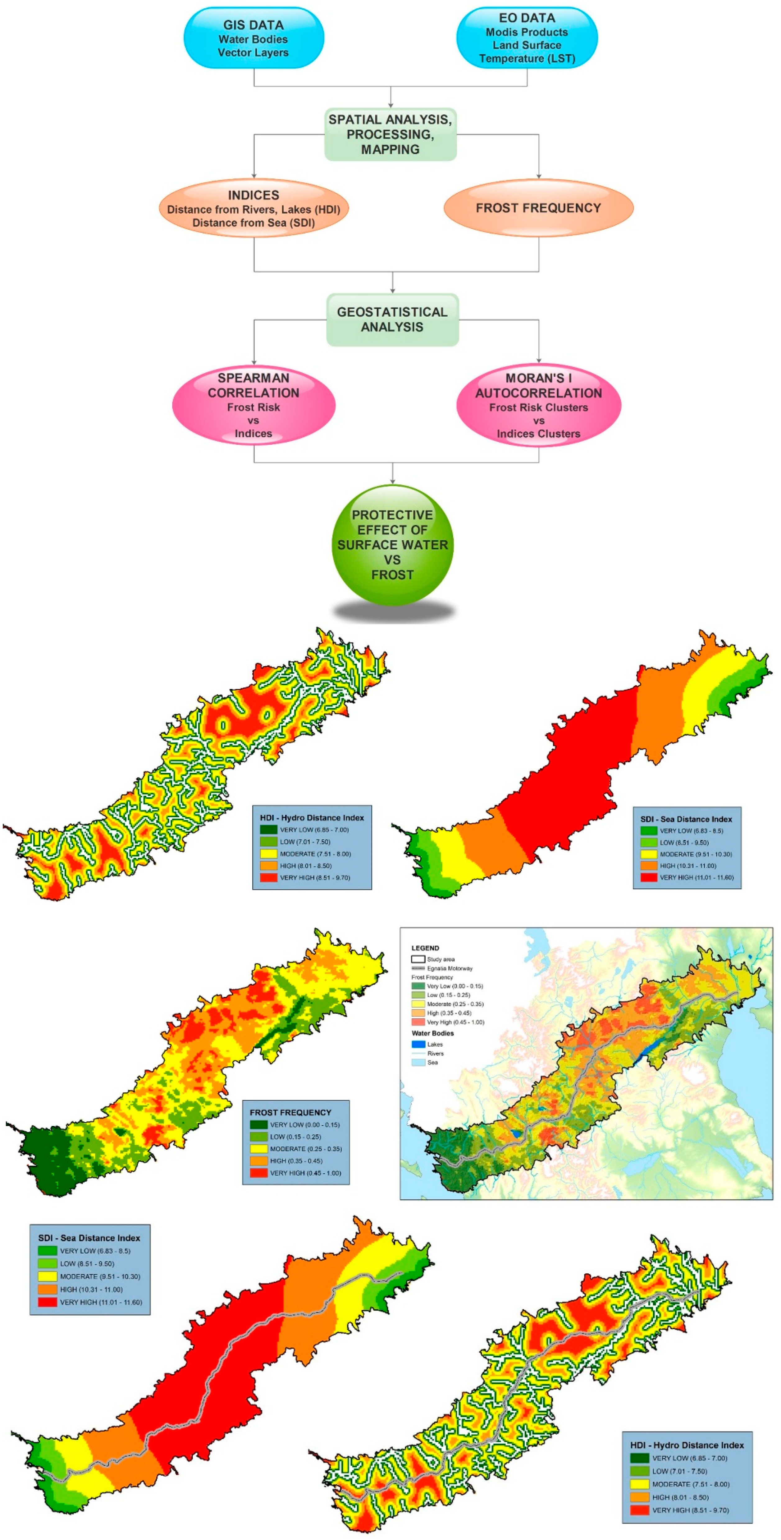
2.4. Frost Monitoring
2.5. Flood Monitoring
2.6. Sea Level Rise Monitoring
3. Contribution of Earth Observation in Natural Disasters
Particularity and Technical Characteristics of EO Satellites
4. Environmental Monitoring, Geospatial Data, and Spatial Data Infrastructures (SDIs)
5. Discussion
6. Conclusions
7. Current Challenges and Future Trends
Author Contributions
Funding
Conflicts of Interest
References
- Karavitis, C. Drought Management Strategies for Urban Water Supplies: The Case of Metropolitan Athens. Ph.D. Thesis, Department of Civil Engineering, Colorado State University, Fort Collins, CO, USA, 1992. [Google Scholar]
- Kalabokidis, K.D.; Karavitis, C.; Vasilakos, C. Automated fire and flood danger assessment system. In Proceedings of the International Workshop on Forest Fires in the Wildland-Urban Interface and Rural Areas in Europe; MAICH: Crete, Greece, 2004; pp. 143–153. [Google Scholar]
- Kalabokidis, K.; Kallos, G.; Karavitis, C.; Caballero, D.; Tettelaar, P.; Llorens, J.; Vasilakos, C. Automated fire and flood hazard protection system. In Proceedings of the 5th International Workshop on Remote Sensing and GIS Applications to Forest Fire Management: Fire Effects Assessment, Zaragoza, Spain, 16–18 June 2005; Universidad de Zaragoza: Zaragoza, Spain, 2005; pp. 167–172. [Google Scholar]
- Tsesmelis, D.E.; Oikonomou, P.D.; Vasilakou, C.G.; Skondras, N.A.; Fassouli, V.; Alexandris, S.G.; Grigg, N.S.; Karavitis, C.A. Assessing structural uncertainty caused by different weighting methods on the Standardized Drought Vulnerability Index (SDVI). Stoch. Environ. Res. Risk Assess. 2019, 33, 515–533. [Google Scholar] [CrossRef]
- Karavitis, C.A.; Tsesmelis, D.E.; Skondras, N.A.; Stamatakos, D.; Alexandris, S.; Fassouli, V.; Vasilakou, C.G.; Oikonomou, P.D.; Gregorič, G.; Grigg, N.S.; et al. Linking drought characteristics to impacts on a spatial and temporal scale. Water Policy 2014, 16, 1172–1197. [Google Scholar] [CrossRef]
- Wilhite, D.A. Chapter 1 Drought as a Natural Hazard: Concepts and Definitions; Drought Mitigation Center Faculty Publications: Lincoln, NE, USA, 2000. [Google Scholar]
- Sonmez, K.; Komuscu, A.U.; Erkan, A.; Turgu, E. An Analysis of Spatial and Temporal Dimension of Drought Vulnerability in Turkey Using the Standardized Precipitation Index. Nat. Hazards 2005, 35, 243–264. [Google Scholar] [CrossRef]
- Grigg, N.S.; Vlachos, E.C. Drought Water Management; International School for Water Resources, Department of Civil Engineering, Colorado State University: Fort Collins, CO, USA, 1990. [Google Scholar]
- Karavitis, C.A. Drought and urban water supplies: The case of metropolitan Athens. Water Policy 1998, 1, 505–524. [Google Scholar] [CrossRef]
- Yevjevich, V.; Da Cunha, L.; Vlachos, E. Coping with Droughts; Water Resources Publications: Littleton, CO, USA, 1983.
- Karavitis, C.A. Decision Support Systems for Drought Management Strategies in Metropolitan Athens. Water Int. 1999, 24, 10–21. [Google Scholar] [CrossRef]
- Bordi, I.; Fraedrich, K.; Petitta, M.; Sutera, A. Large-Scale Assessment of Drought Variability Based on NCEP/NCAR and ERA-40 Re-Analyses. Water Resour. Manag. 2006, 20, 899–915. [Google Scholar] [CrossRef] [Green Version]
- Mishra, A.K.; Singh, V.P. A review of drought concepts. J. Hydrol. 2010, 391, 202–216. [Google Scholar] [CrossRef]
- Oikonomou, P.D.; Tsesmelis, D.E.; Waskom, R.M.; Grigg, N.S.; Karavitis, C.A. Enhancing the Standardized Drought Vulnerability Index by Integrating Spatiotemporal Information from Satellite and In Situ Data. J. Hydrol. 2019, 569, 265–277. [Google Scholar] [CrossRef]
- Adger, W.N. Vulnerability. Glob. Environ. Chang. 2006, 16, 268–281. [Google Scholar] [CrossRef]
- Horton, G.; Hanna, L.; Kelly, B. Drought, drying and climate change: Emerging health issues for ageing Australians in rural areas. Australas. J. Ageing 2010, 29, 2–7. [Google Scholar] [CrossRef]
- Wilhite, D.A.; Sivakumar, M.V.K.; Pulwarty, R. Managing drought risk in a changing climate: The role of national drought policy. Weather Clim. Extrem. 2014, 3, 4–13. [Google Scholar] [CrossRef] [Green Version]
- Ciais, P.; Reichstein, M.; Viovy, N.; Granier, A.; Ogée, J.; Allard, V.; Aubinet, M.; Buchmann, N.; Bernhofer, C.; Carrara, A.; et al. Europe-wide reduction in primary productivity caused by the heat and drought in 2003. Nature 2005, 437, 529–533. [Google Scholar] [CrossRef]
- Oikonomou, P.D.; Karavitis, C.A.; Tsesmelis, D.E.; Kolokytha, E.; Maia, R. Drought Characteristics Assessment in Europe over the Past 50 Years. Water Resources Management. 2020, 34, 4757–4772. [Google Scholar] [CrossRef]
- Tsesmelis, D.E. Development, Implementation and Evaluation of Drought and Desertification Risk Indicators for the Integrated Management of Water Resources. Ph.D. Thesis, Department of Natural Resources Management & Agricultural Engineering, Agricultural University of Athens, Athens, Greece, 2017. [Google Scholar]
- Karavitis, C.A.; Alexandris, S.; Tsesmelis, D.E.; Athanasopoulos, G. Application of the Standardized Precipitation Index (SPI) in Greece. Water 2011, 3, 787–805. [Google Scholar] [CrossRef]
- Karavitis, C.A.; Chortaria, C.; Alexandris, S.; Vasilakou, C.G.; Tsesmelis, D.E. Development of the standardised precipitation index for Greece. Urban. Water J. 2012, 9, 401–417. [Google Scholar] [CrossRef]
- Pedro-Monzonís, M.; Ferrer, J.; Solera, A.; Estrela, T.; Paredes-Arquiola, J. Key issues for determining the exploitable water resources in a Mediterranean river basin. Sci. Total Environ. 2015, 503–504, 319–328. [Google Scholar]
- Pedro-Monzonís, M.; Solera, A.; Ferrer, J.; Estrela, T.; Paredes-Arquiola, J. A review of water scarcity and drought indexes in water resources planning and management. J. Hydrol. 2015, 527, 482–493. [Google Scholar] [CrossRef] [Green Version]
- Loucks, D.P. Sustainable Water Resources Management. Water Int. 2000, 25, 3–10. [Google Scholar] [CrossRef]
- Wilhite, D.A.; Hayes, M.J.; Knutson, C.; Smith, K.H. Planning for drought: Moving from crisis to risk management. JAWRA J. Am. Water Resour. Assoc. 2000, 36, 697–710. [Google Scholar] [CrossRef]
- Kampragou, E.; Apostolaki, S.; Manoli, E.; Froebrich, J.; Assimacopoulos, D. Towards the harmonization of water-related policies for managing drought risks across the EU. Environ. Sci. Policy 2011, 14, 815–824. [Google Scholar] [CrossRef]
- Skondras, N.A.; Karavitis, C.A.; Gkotsis, I.I.; Scott, P.J.B.; Kaly, U.L.; Alexandris, S.G. Application and assessment of the Environmental Vulnerability Index in Greece. Ecol. Indic. 2011, 11, 1699–1706. [Google Scholar] [CrossRef]
- Skondras, N. Decision Making in Water Resources Management: Development of a Composite Indicator for the Assessment of the Social-Environmental Systems in Terms Resilience and Vulnerability to Water Scarcity and Water Stress. Ph.D. Thesis, Department of Natural Resources Management and Agricultural Engineering, Agricultural University of Athens, Athens, Greece, 2015. [Google Scholar]
- Cancelliere, A.; Mauro, G.D.; Bonaccorso, B.; Rossi, G. Drought forecasting using the Standardized Precipitation Index. Water Resour. Manag. 2007, 21, 801–819. [Google Scholar] [CrossRef]
- Priscoli, J.D. Keynote Address: Clothing the IWRM Emperor by Using Collaborative Modeling for Decision Support. JAWRA J. Am. Water Resour. Assoc. 2013, 49, 609–613. [Google Scholar] [CrossRef]
- Salas, J.D.; Fu, C.; Cancelliere, A.; Dustin, D.; Bode, D.; Pineda, A.; Vincent, E. Characterizing the Severity and Risk of Drought in the Poudre River, Colorado. J. Water Resour. Plan. Manag. 2005, 131, 383–393. [Google Scholar] [CrossRef]
- Vlachos, E. Prologue: Water peace and conflict management. Water Int. 1990, 15, 185–188. [Google Scholar]
- Vlachos, E.; Braga, B. The challenge of urban water management. In Proceedings of the Frontiers in Urban Water Management: Deadlock or Hope; IWA Publishing: London, UK, 2001; pp. 1–36. [Google Scholar]
- Grigg, N.S. Water Resources Management. In Water Encyclopedia; John Wiley & Sons, Inc.: Hoboken, NJ, USA, 1996. [Google Scholar]
- Tsesmelis, D.E.; Karavitis, C.A.; Oikonomou, P.D.; Alexandris, S.; Kosmas, C. Assessment of the Vulnerability to Drought and Desertification Characteristics Using the Standardized Drought Vulnerability Index (SDVI) and the Environmentally Sensitive Areas Index (ESAI). Resources 2019, 8, 6. [Google Scholar] [CrossRef] [Green Version]
- Swathandran, S.; Aslam, M.A.M. Assessing the role of SWIR band in detecting agricultural crop stress: A case study of Raichur district, Karnataka, India. Environ. Monit. Assess. 2019, 191, 442. [Google Scholar] [CrossRef] [PubMed]
- Vlachos, E.C. Drought Management Interfaces; ASCE: Las Vegas, NE, USA, 1982; p. 15. [Google Scholar]
- AghaKouchak, A.; Feldman, D.; Hoerling, M.; Huxman, T.; Lund, J. Water and climate: Recognize anthropogenic drought. Nat. News 2015, 524, 409. [Google Scholar] [CrossRef] [Green Version]
- Tsakiris, G.; Pangalou, D.; Vangelis, H. Regional Drought Assessment Based on the Reconnaissance Drought Index (RDI). Water Resour. Manag. 2007, 21, 821–833. [Google Scholar] [CrossRef]
- Vangelis, H.; Tigkas, D.; Tsakiris, G. The effect of PET method on Reconnaissance Drought Index (RDI) calculation. J. Arid Environ. 2013, 88, 130–140. [Google Scholar] [CrossRef]
- Fassouli, V. Development, Implementation and Assessment of a Composite Index for the Identification and Classification of Drought and Creation of the Corresponding Decision Support System. Ph.D. Thesis, Department of Natural Resources Management & Agricultural Engineering, Agricultural University of Athens, Athens, Greece, 2017. [Google Scholar]
- Rossi, G.; Benedini, M.; Tsakiris, G.; Giakoumakis, S. On regional drought estimation and analysis. Water Resour. Manag. 1992, 6, 249–277. [Google Scholar] [CrossRef]
- Pimentel, D. Soil erosion: A food and environmental threat. Environ. Dev. Sustain. 2006, 8, 119–137. [Google Scholar] [CrossRef]
- Lal, R. Soil erosion and the global carbon budget. Environ. Int. 2003, 29, 437–450. [Google Scholar] [CrossRef]
- Milliman, J.D.; Syvitski, J.P.M. Geomorphic/tectonic control of sediment discharge to the ocean: The importance of small mountainous rivers. J. Geol. 1992, 100, 525–544. [Google Scholar] [CrossRef]
- Walling, D.E.; Webb, B.W. Erosion and sediment yield: A global overview. In Erosion and Sediment Yield: Global and Regional Perspectives Proceedings of the Exeter Symposium; Walling, D.E., Webb, B.W., Eds.; IAHS Publication No. 236; ISI: Exeter, UK, 1996; pp. 3–19. [Google Scholar]
- Polykretis, C.; Alexakis, D.D.; Grillakis, M.G.; Manoudakis, S. Assessment of Intra-Annual and Inter-Annual Variabilities of Soil Erosion in Crete Island (Greece) by Incorporating the Dynamic “Nature” of R and C-Factors in RUSLE Modeling. Remote Sens. 2020, 12, 2439. [Google Scholar] [CrossRef]
- Lai, R. Soil degradation by erosion. Land Degrad. Dev. 2001, 12, 519–539. [Google Scholar]
- Xu, L.; Xu, X.; Meng, X. Risk assessment of soil erosion in different rainfall scenarios by RUSLE model coupled with Information Diffusion Model: A case study of Bohai Rim, China. Catena 2013, 100, 74–82. [Google Scholar] [CrossRef]
- Nearing, M.A.; Pruski, F.F.; O’neal, M.R. Expected climate change impacts on soil erosion rates: A review. J. Soil Water Conserv. 2004, 59, 43–50. [Google Scholar]
- Ganasri, B.P.; Ramesh, H. Assessment of soil erosion by RUSLE model using remote sensing and GIS-A case study of Nethravathi Basin. Geosci. Front. 2016, 7, 953–961. [Google Scholar] [CrossRef] [Green Version]
- Oldeman, L.R.; Van Engelen, V.W.P.; Pulles, J.H.M. The extent of human induced soil degradation. In Annex 5 of World Man of the Status of Human-Induced Soil Degradation: An. Explanatory Note, 2nd ed.; Oldeman, L.R., Hakkeling, R.T.A., Sombroek, W.G., Eds.; International Soil Reference and Information Center: Wageningen, The Netherlands, 1990. [Google Scholar]
- Fistikoglu, O.; Harmancioglu, N.B. Integration of GIS with USLE in assessment of soil erosion. Water Resour. Manag. 2002, 16, 447–467. [Google Scholar] [CrossRef]
- Kothyari, U.C. Erosion and sediment problems in India. In Proceedings of the Exeter Symposium on Erosion and Sediment Yield: Global and Regional Perspectives; IAHS Publication No. 236; ISI: Exeter, UK, 1996; pp. 531–540. [Google Scholar]
- Jha, M.K.; Paudel, R.C. Erosion predictions by empirical models in a mountainous watershed in Nepal. J. Spat. Hydrol. 2010, 10, 89–102. [Google Scholar]
- Wischmeier, W.H.; Smith, D.D. Predicting Rainfall Erosion Losses: A Guide to Conservation Planning; Agriculture Handbook No. 537; USDA: Washington, DC, USA, 1978.
- Karydas, C.G.; Panagos, P.; Gitas, I.Z. A classification of water erosion models according to their geospatial characteristics. Int. J. Digit. Earth 2014, 7, 229–250. [Google Scholar] [CrossRef]
- Zhang, Z.-H.; Gang, H.U.; Jian, N.I. Effects of Topographical and Edaphic Factors on the Distribution of Plant Communities in Two Subtropical Karst Forests, Southwestern China. J. Mt. Sci. 2013, 10, 95–104. [Google Scholar] [CrossRef]
- Lee, G.S.; Lee, K.H. Scaling effect for estimating soil loss in the RUSLE model using remotely sensed geospatial data in Korea. J. Hydrol. Earth Syst. Sci. 2006, 3, 135–157. [Google Scholar]
- Remortel Van, R.; Hamilton, M.; Hickey, R. Estimating the LS factor for RUSLE through iterative slope length processing of digital elevation data. Cartography 2001, 30, 27–35. [Google Scholar] [CrossRef]
- Eckelmann, W.; Baritz, R.; Bialousz, S.; Bielek, P.; Carré, F.; Hrušková, B.; Jones, R.J.; Kibblewhite, M.; Kozak, J.; Le Bas, C.; et al. Common Criteria for Risk Area Identification According to Soil Threats; Office for Official Publications of the European Communities: Brussels, Belgium, 2006. [Google Scholar]
- Van Beek, C.L.; Tóth, T.; Hagyó, A.; Tóth, G.; Recatalá Boix, L.; Añó Vidal, C.; Malet, J.P.; Maquaire, O.; Van den Akker, J.J.H.; Van der Zee, S.; et al. The need for harmonizing methodologies for assessing soil threats in Europe. Soil Use Manag. 2010, 26, 299–309. [Google Scholar] [CrossRef]
- Rozos, D.; Skilodimou, H.D.; Loupasakis, C.; Bathrellos, G.D. Application of the revised universal soil loss equation model on landslide prevention. An example from N. Euboea (Evia) Island, Greece. Environ. Earth Sci. 2013, 70, 3255–3266. [Google Scholar] [CrossRef]
- Fernandez, P.; Delgado, E.; Lopez-Alonso, M.; Poyatos, J.M. GIS environmental information analysis of the Darro River basin as the key for the management and hydrological forest restoration. Sci. Total Environ. 2018, 613, 1154–1164. [Google Scholar] [CrossRef]
- De Jong, S.M. Applications of reflective remote sensing for land degradation studies in a Mediterranean environment. Ph.D. Thesis, Utrecht University, Utrecht, The Netherlands, 1994. [Google Scholar]
- De Vente, J.; Poesen, J. Predicting soil erosion and sediment yield at the basin scale: Scale issues and semi-quantitative models. Earth Sci. Rev. 2005, 71, 95–125. [Google Scholar] [CrossRef]
- Giordano, A.; Bonfils, P.; Briggs, D.J.; de Sequeira, E.M.; de Laburu, C.R.; Yassoglou, N. The methodological approach to soil erosion and important land resources evaluation of the European Community. Soil Technol. 1991, 4, 65–77. [Google Scholar] [CrossRef]
- Stathopoulos, N.; Lykoudi, E.; Vasileiou, E.; Rozos, D.; Dimitrakopoulos, D. Erosion Vulnerability Assessment of Sperchios River Basin, in East Central Greece—A GIS Based Analysis. Open J. Geol. 2017, 7, 621–646. [Google Scholar] [CrossRef] [Green Version]
- Gitas, Ι.Z.; Douros, K.; Minakou, C.; Silleos, G.N.; Karydas, C.G. Multi-temporal soil erosion risk assessment in N. Chalkidiki using a modified USLE raster model. EARSeL eProceedings 2009, 8, 40–52. [Google Scholar]
- Fernandez, C.; Wu, J.Q.; McCool, D.Q.; Stockle, C.O. Estimating water erosion and sediment yield with GIS, RUSLE and SEDD. J. Soil Water Conserv. 2003, 58, 128–136. [Google Scholar]
- Alemayehu, F.; Taha, N.; Nyssen, J.; Girma, A.; Zenebe, A.; Behailu, M.; Deckers, S.; Poesen, J. The impacts of watershed management on land use and land cover dynamics in Eastern Tigray (Ethiopia). Resour. Conserv. Recycl. 2009, 53, 192–198. [Google Scholar] [CrossRef]
- Rahman, M.R.; Shi, Z.H.; Chongfa, C. Soil erosion hazard evaluation—An integrated use of remote sensing, GIS and statistical approaches with biophysical parameters towards management strategies. Ecol. Model. 2009, 220, 1724–1734. [Google Scholar] [CrossRef]
- Alexakis, D.D.; Hadjimitsis, D.G.; Agapiou, A. Integrated use of remote sensing, GIS and precipitation data for the assessment of soil erosion rate in the catchment area of “Yialias” in Cyprus. Atmos. Res. 2013, 131, 108–124. [Google Scholar] [CrossRef]
- Künzer, C.; Ottinger, M.; Liu, G.; Sun, B.; Baumhauer, R.; Dech, S. Earth observation-based coastal zone monitoring of the Yellow River Delta: Dynamics in China’s second largest oil producing region over four decades. Appl. Geogr. 2014, 55, 92–107. [Google Scholar] [CrossRef]
- Alexandridis, T.K.; Sotiropoulou, A.M.; Bilas, G.; Karapetsas, N.; Silleos, N.G. The Effects of Seasonality in Estimating the C-Factor of Soil Erosion Studies. Land Degrad. Dev. 2015, 26, 596–603. [Google Scholar] [CrossRef]
- Ghosh, M.K.; Kumar, L.; Roy, C. Monitoring the coastline change of Hatiya Island in Bangladesh using remote sensing techniques. ISPRS J. Photogramm. Remote Sens. 2015, 101, 137–144. [Google Scholar] [CrossRef]
- AbdelRahman, M.A.; Natarajan, A.; Hegde, R. Assessment of land suitability and capability by integrating remote sensing and GIS for agriculture in Chamarajanagar district, Karnataka, India. Egypt. J. Remote Sens. Space Sci. 2016, 19, 125–141. [Google Scholar] [CrossRef] [Green Version]
- Neugirg, F.; Stark, M.; Kaiser, A.; Vlacilova, M.; Della Seta, M.; Vergari, F.; Schmidt, J.; Becht, M.; Haas, F. Erosion processes in calanchi in the Upper Orcia Valley, Southern Tuscany, Italy based on multitemporal high-resolution terrestrial LiDAR and UAV surveys. Geomorphology 2016, 269, 8–22. [Google Scholar] [CrossRef]
- Rayegani, B.; Barati, S.; Sohrabi, T.A.; Sonboli, B. Remotely sensed data capacities to assess soil degradation. Egypt. J. Remote Sens. Space Sci. 2016, 19, 207–222. [Google Scholar] [CrossRef] [Green Version]
- Dewan, A.; Corner, R.; Saleem, A.; Rahman, M.M.; Haider, M.R.; Rahman, M.M.; Sarker, M.H. Assessing channel changes of the Ganges-Padma River system in Bangladesh using Landsat and hydrological data. Geomorphology 2017, 276, 257–279. [Google Scholar] [CrossRef]
- Chappell, A.; Webb, N.P.; Guerschman, J.P.; Thomas, D.T.; Mata, G.; Handcock, R.N.; Leys, J.F.; Butler, H.J. Improving ground cover monitoring for wind erosion assessment using MODIS BRDF parameters. Remote Sens. Environ. 2018, 204, 756–768. [Google Scholar] [CrossRef]
- Nigel, R.; Rughooputh, S. Mapping of monthly soil erosion risk of mainland Mauritius and its aggregation with delineated basins. Geomorphology 2010, 114, 101–114. [Google Scholar] [CrossRef]
- Jain, M.K.; Das, D. Estimation of sediment yield and areas of soil erosion and deposition for watershed prioritization using GIS and remote sensing. Water Resour. Manag. 2010, 24, 2091–2112. [Google Scholar] [CrossRef]
- Chou, W.C. Modelling watershed scale soil loss prediction and sediment yield estimation. Water Resour. Manag. 2010, 24, 2075–2090. [Google Scholar] [CrossRef]
- Hui, L.; Xiaoling, C.; Lim, K.J.; Xiaobin, C.; Sagong, M. Assessment of soil erosion and sediment yield in Liao watershed, Jiangxi Province, China, Using USLE, GIS, and RS. J. Earth Sci. 2010, 21, 941–953. [Google Scholar] [CrossRef]
- Ouyang, W.; Hao, F.; Skidmore, A.K.; Toxopeus, A.G. Soil erosion and sediment yield and their relationships with vegetation cover in upper stream of the Yellow River. Sci. Total Environ. 2010, 409, 396–403. [Google Scholar] [CrossRef]
- Demirci, A.; Karaburun, A. Estimation of soil erosion using RUSLE in a GIS framework: A case study in the Buyukcekmece Lake watershed, northwest Turkey. Environ. Earth Sci. 2012, 66, 903–913. [Google Scholar] [CrossRef]
- Mhangara, P.; Kakembo, V.; Lim, K.J. Soil erosion risk assessment of the Keiskamma catchment, South Africa using GIS and remote sensing. Environ. Earth Sci. 2012, 65, 2087–2102. [Google Scholar] [CrossRef]
- Pradhan, B.; Chaudhari, A.; Adinarayana, J.; Buchroithner, M.F. Soil erosion assessment and its correlation with landslide events using remote sensing data and GIS: A case study at Penang Island, Malaysia. Environ. Monit. Assess. 2012, 184, 715–727. [Google Scholar] [CrossRef] [PubMed]
- Prasannakumar, V.; Vijith, H.; Abinod, S.; Geetha, N. Estimation of soil erosion risk within a small mountainous sub-watershed in Kerala, India, using Revised Universal Soil Loss Equation (RUSLE) and geo-information technology. Geosci. Front. 2012, 3, 209–215. [Google Scholar] [CrossRef] [Green Version]
- Ranzi, R.; Le, T.H.; Rulli, M.C. A RUSLE approach to model suspended sediment load in the Lo river (Vietnam): Effects of reservoirs and land use changes. J. Hydrol. 2012, 422, 17–29. [Google Scholar] [CrossRef]
- Esteves, T.C.J.; Kirkby, M.J.; Shakesby, R.A.; Ferreira, A.J.D.; Soares, J.A.A.; Irvine, B.J.; Ferreira, C.S.S.; Coelho, C.O.A.; Bento, C.P.M.; Carreiras, M.A. Mitigating land degradation caused by wildfire: Application of the PESERA model to fire-affected sites in central Portugal. Geoderma 2012, 191, 40–50. [Google Scholar] [CrossRef]
- Chatterjee, S.; Krishna, A.P.; Sharma, A.P. Geospatial assessment of soil erosion vulnerability at watershed level in some sections of the Upper Subarnarekha river basin, Jharkhand, India. Environ. Earth Sci. 2014, 71, 357–374. [Google Scholar] [CrossRef]
- Sun, W.; Shao, Q.; Liu, J.; Zhai, J. Assessing the effects of land use and topography on soil erosion on the Loess Plateau in China. Catena 2014, 121, 151–163. [Google Scholar] [CrossRef]
- Cilek, A.; Berberoglu, S.; Kirkby, M.; Irvine, B.; Donmez, C.; Erdogan, M.A. Erosion modelling in a Mediterranean subcatchment under climate change scenarios using Pan-European Soil Erosion Risk Assessment (PESERA). Int. Arch. Photogramm. Remote Sens. Spat. Inf. Sci. 2015, 40, 359. [Google Scholar] [CrossRef] [Green Version]
- Aiello, A.; Adamo, M.; Canora, F. Remote sensing and GIS to assess soil erosion with RUSLE3D and USPED at river basin scale in southern Italy. Catena 2015, 131, 174–185. [Google Scholar] [CrossRef]
- Gaubi, I.; Chaabani, A.; Mammou, A.B.; Hamza, M.H. A GIS-based soil erosion prediction using the Revised Universal Soil Loss Equation (RUSLE) (Lebna watershed, Cap Bon, Tunisia). Nat. Hazards 2017, 86, 219–239. [Google Scholar] [CrossRef]
- Bera, A. Estimation of soil loss by USLE model using GIS and remote sensing techniques: A case study of Muhuri River Basin, Tripura, India. Eurasian J. Soil Sci. 2017, 6, 206. [Google Scholar] [CrossRef] [Green Version]
- Bouguerra, H.; Bouanani, A.; Khanchoul, K.; Derdous, O.; Tachi, S.E. Mapping erosion prone areas in the Bouhamdane watershed (Algeria) using the Revised Universal Soil Loss Equation through GIS. J. Water Land Dev. 2017, 32, 13–23. [Google Scholar] [CrossRef]
- Karydas, C.G.; Panagos, P. The G2 erosion model: An algorithm for month-time step assessments. Environ. Res. 2018, 161, 256–267. [Google Scholar] [CrossRef]
- Leh, M.; Bajwa, S.; Chaubey, I. Impact of land use change on erosion risk: An integrated remote sensing, geographic information system and modeling methodology. Land Degrad. Dev. 2013, 24, 409–421. [Google Scholar] [CrossRef]
- Park, S.; Oh, C.; Jeon, S.; Jung, H.; Choi, C. Soil erosion risk in Korean watersheds, assessed using the revised universal soil loss equation. J. Hydrol. 2011, 399, 263–273. [Google Scholar] [CrossRef]
- Chowdary, V.M.; Chakraborthy, D.; Jeyaram, A.; Murthy, Y.K.; Sharma, J.R.; Dadhwal, V.K. Multi-criteria decision making approach for watershed prioritization using analytic hierarchy process technique and GIS. Water Resour. Manag. 2013, 27, 3555–3571. [Google Scholar] [CrossRef]
- Badar, B.; Romshoo, S.A.; Khan, M.A. Integrating biophysical and socioeconomic information for prioritizing watersheds in a Kashmir Himalayan lake: A remote sensing and GIS approach. Environ. Monit. Assess. 2013, 185, 6419–6445. [Google Scholar] [CrossRef]
- Mello, C.D.; Viola, M.R.; Beskow, S.; Norton, L.D. Multivariate models for annual rainfall erosivity in Brazil. Geoderma 2013, 202, 88–102. [Google Scholar] [CrossRef]
- Thomas, J.; Joseph, S.; Thrivikramji, K.P. Assessment of soil erosion in a tropical mountain river basin of the southern Western Ghats, India using RUSLE and GIS. Geosci. Front. 2018, 9, 893–906. [Google Scholar] [CrossRef]
- Macedo, D.R.; Hughes, R.M.; Kaufmann, P.R.; Callisto, M. Development and validation of an environmental fragility index (EFI) for the neotropical savannah biome. Sci. Total Environ. 2018, 635, 1267–1279. [Google Scholar] [CrossRef]
- Tetzlaff, B.; Friedrich, K.; Vorderbrügge, T.; Vereecken, H.; Wendland, F. Distributed modelling of mean annual soil erosion and sediment delivery rates to surface waters. Catena 2013, 102, 13–20. [Google Scholar] [CrossRef]
- Shi, Z.H.; Cai, C.F.; Ding, S.W.; Wang, T.W.; Chow, T.L. Soil conservation planning at the small watershed level using RUSLE with GIS: A case study in the Three Gorge Area of China. Catena 2004, 55, 33–48. [Google Scholar] [CrossRef]
- Şahin, Ş.; Kurum, E. Erosion risk analysis by GIS in environmental impact assessments: A case study—Seyhan Köprü Dam construction. J. Environ. Manag. 2002, 66, 239–247. [Google Scholar] [CrossRef]
- Millward, A.A.; Mersey, J.E. Conservation strategies for effective land management of protected areas using an erosion prediction information system (EPIS). J. Environ. Manag. 2001, 61, 329–343. [Google Scholar] [CrossRef] [PubMed]
- Aguirre, J.A.M.; Sánchez, J.C.R. Caracterización de las cuencas hidrográficas, objeto de restauración higrológico-forestal, mediante modelos hidrológicos. Ing. Del Agua 1994, 1, 2. [Google Scholar]
- Tabesh, M.; Saber, H. A prioritization model for rehabilitation of water distribution networks using GIS. Water Resour. Manag. 2012, 26, 225–241. [Google Scholar] [CrossRef]
- Tang, Z.; Li, X.; Zhao, N.; Li, R.; Harvey, E.F. Developing a restorable wetland index for rainwater basin wetlands in south-central Nebraska: A multi-criteria spatial analysis. Wetlands 2012, 32, 975–984. [Google Scholar] [CrossRef]
- Nekhay, O.; Arriaza, M.; Boerboom, L. Evaluation of soil erosion risk using Analytic Network Process and GIS: A case study from Spanish mountain olive plantations. J. Environ. Manag. 2009, 90, 3091–3104. [Google Scholar] [CrossRef]
- De Paz, J.M.; Sánchez, J.; Visconti, F. Combined use of GIS and environmental indicators for assessment of chemical, physical and biological soil degradation in a Spanish Mediterranean region. J. Environ. Manag. 2006, 79, 150–162. [Google Scholar] [CrossRef]
- Liu, C.; Frasier, P.; Kumar, L.; Macgregor, C. Catchmentwide wetland assessment and prioritization using the multi-criteria decision making method TOPIS. Environ. Manag. 2006, 38, 316–326. [Google Scholar] [CrossRef] [PubMed]
- Metternicht, G.; Gonzalez, S. FUERO: Foundations of a fuzzy exploratory model for soil erosion hazard prediction. Environ. Model. Softw. 2005, 20, 715–728. [Google Scholar] [CrossRef]
- Navas, A.; Machín, J.; Soto, J. Assessing soil erosion in a Pyrenean mountain catchment using GIS and fallout 137Cs. Agric. Ecosyst. Environ. 2005, 105, 493–506. [Google Scholar] [CrossRef] [Green Version]
- Finlayson, D.P.; Montgomery, D.R. Modelling large-scale fluvial erosion in geographic information systems. Geomorphology 2003, 53, 147–164. [Google Scholar] [CrossRef]
- Chowdhury, A.; Jha, M.K.; Chowdary, V.M.; Mal, B.C. Integrated remote sensing and GIS-based approach for assessing groundwater potential in West Medinipur district, West Bengal, India. Int. J. Remote Sens. 2009, 30, 231–250. [Google Scholar] [CrossRef]
- Magesh, N.S.; Chandrasekar, N.; Soundranayagam, J.P. Delineation of groundwater potential zones in Theni district, Tamil Nadu, using remote sensing, GIS and MIF techniques. Geosci. Front. 2012, 3, 189–196. [Google Scholar] [CrossRef] [Green Version]
- Babiker, I.S.; Mohamed, M.A.; Hiyama, T. Assessing groundwater quality using GIS. Water Resour. Manag. 2007, 21, 699–715. [Google Scholar] [CrossRef]
- Mukherjee, S.; Veer, V.; Tyagi, S.K.; Sharma, V. Sedimentation study of Hirakud reservoir through remote sensing techniques. J. Spat. Hydrol. 2007, 7, 1. [Google Scholar]
- Saraf, A.K.; Choudhury, P.R. Integrated remote sensing and GIS for groundwater exploration and identification of artificial recharge sites. Int. J. Remote Sens. 1998, 19, 1825–1841. [Google Scholar] [CrossRef]
- Babiker, I.S.; Mohamed, M.A.; Terao, H.; Kato, K.; Ohta, K. Assessment of groundwater contamination by nitrate leaching from intensive vegetable cultivation using geographical information system. Environ. Int. 2004, 29, 1009–1017. [Google Scholar] [CrossRef]
- Shetkar, R.V.; Mahesha, A. Tropical, seasonal river basin development: Hydrogeological analysis. J. Hydrol. Eng. 2004, 16, 280–291. [Google Scholar] [CrossRef]
- Sener, E.; Davraz, A.; Ozcelik, M. An integration of GIS and remote sensing in groundwater investigations: A case study in Burdur, Turkey. Hydrogeol. J. 2005, 13, 826–834. [Google Scholar] [CrossRef]
- Engman, E.T.; Gurney, R.J. Remote Sensing in Hydrology; Chapman and Hall: London, UK, 1991. [Google Scholar]
- Jha, M.K.; Chowdhury, A.; Chowdary, V.M.; Peiffer, S. Groundwater management and development by integrated remote sensing and geographic information systems: Prospects and constraints. Water Resour. Manag. 2007, 21, 427–467. [Google Scholar] [CrossRef]
- Todd, D.K. Groundwater Hydrogeology, 2nd ed.; John Wiley & Son: New York, NY, USA, 1980. [Google Scholar]
- Jha, M.K.; Peiffer, S. Applications of Remote Sensing and GIS Technologies in Groundwater Hydrology: Past, Present and Future; BayCEER: Bayreuth, Germany, 2006; p. 201. [Google Scholar]
- Tiwari, A.; Rai, B. Hydromorphogeological mapping for groundwater prospecting using landsat-MSS images—a case study of part of Dhanbad District, Bihar. J. Indian Soc. Remote Sens. 1996, 24, 281–285. [Google Scholar] [CrossRef]
- Das, S.; Behera, S.C.; Kar, A.; Narendra, P.; Guha, S. Hydrogeomorphological mapping in ground water exploration using remotely sensed data—a case study in keonjhar district, orissa. J. Indian Soc. Remote Sens. 1997, 25, 247–259. [Google Scholar] [CrossRef]
- Thomas, A.; Sharma, P.K.; Sharma, M.K.; Sood, A. Hydrogeomorphological mapping in assessing ground water by using remote sensing data—A case study in lehra gaga block, sangrur district, Punjab. J. Indian Soc. Remote Sens. 1999, 27, 31. [Google Scholar] [CrossRef]
- Harinarayanan, P.; Gopalakrishna, G.S.; Balasubramanian, A. Remote sensing data for groundwater development and management in Keralapura watersheds of Cauvery Basin, Karnataka, India. Indian Mineral. 2000, 34, 11–17. [Google Scholar]
- Muralidhar, M.; Raju, K.R.K.; Raju, K.S.V.P.; Prasad, J.R. Remote sensing applications for the evaluation of water resources in rainfed area, Warangal district, Andhra Pradesh. Indian Miner. 2000, 34, 33–40. [Google Scholar]
- Chowdhury, A.; Jha, M.K.; Chowdary, V.M. Delineation of groundwater recharge zones and identification of artificial recharge sites in West Medinipur district, West Bengal, using RS, GIS and MCDM techniques. Environ. Earth Sci. 2010, 59, 1209. [Google Scholar] [CrossRef]
- Stafford, D.B. Civil Engineering Applications of Remote Sensing and Geographic Information Systems; ASCE: Reston, VA, USA, 1991. [Google Scholar]
- Goodchild, M.F. The state of GIS for environmental problem-solving. In Environmental Modeling with GIS; IntechOpen: London, UK, 1993; pp. 8–15. [Google Scholar]
- Chopra, R.; Sharma, P.K. Landform analysis and ground water potential in the Bist Doab area, Punjab, India. Int. J. Remote Sens. 1993, 14, 3221–3229. [Google Scholar] [CrossRef]
- Sander, P. Water-well siting in hard-rock areas: Identifying promising targets using a probabilistic approach. Hydrogeol. J. 1997, 5, 32–43. [Google Scholar] [CrossRef]
- Teeuw, R.M. Groundwater exploration using remote sensing and a low-cost geographical information system. Hydrogeol. J. 1995, 3, 21–30. [Google Scholar] [CrossRef]
- Dar, I.A.; Sankar, K.; Dar, M.A. Deciphering groundwater potential zones in hard rock terrain using geospatial technology. Environ. Monit. Assess. 2011, 173, 597–610. [Google Scholar] [CrossRef] [PubMed]
- Kumar, S.K.; Chandrasekar, N.; Seralathan, P.; Godson, P.S.; Magesh, N.S. Hydrogeochemical study of shallow carbonate aquifers, Rameswaram Island, India. Environ. Monit. Assess. 2012, 184, 4127–4138. [Google Scholar] [CrossRef]
- Jankowski, P. Integrating geographical information systems and multiple criteria decision-making methods. Int. J. Geogr. Inf. Syst. 1995, 9, 251–273. [Google Scholar] [CrossRef]
- Solomon, S.; Quiel, F. Groundwater study using remote sensing and geographic information systems (GIS) in the central highlands of Eritrea. Hydrogeol. J. 2006, 14, 229–741. [Google Scholar] [CrossRef] [Green Version]
- Prasad, R.K.; Mondal, N.C.; Banerjee, P.; Nandakumar, M.V.; Singh, V.S. Deciphering potential groundwater zone in hard rock through the application of GIS. Environ. Geol. 2008, 55, 467–475. [Google Scholar] [CrossRef]
- Gustafsson, P. High Resolution Satellite Imagery and GIS as a Dynamic Tool in Groundwater Exploration in a Semi-arid Area; IAHS Publication: Wallingford, UK, 1993. [Google Scholar]
- Snyder, R.L.; Melo-Abreu, J.D. Frost Protection: Fundamentals, Practice and Economics; Food and Agriculture Organization of the United Nations: Rome, Italy, 2005; Volume 1, pp. 1–240.
- Kramer, P.J. Water Relations of Plants; Academic Press: San Diego, CA, USA, 1983. [Google Scholar]
- Waring, R.H.; Schlesinger, W.H. Forest Ecosystems, Concepts and Management; Academic Press: Orlando, FL, USA, 1985. [Google Scholar]
- Aber, J.D.; Melillo, J.M. Terrestrial Ecosystems; Saunders College Publishing: Philadelphia, PA, USA, 1991. [Google Scholar]
- Blennow, K.; Lindkvist, L. Models of low temperature and high irradiance and their application to explaining the risk of seedling mortality. For. Ecol. Manag. 2000, 135, 289–301. [Google Scholar] [CrossRef]
- Thornes, J.E. Road salting—An international cost/benefit review. In 8th World Salt Symposium; Geertman, R.M., Ed.; Elsevier: Amsterdam, The Netherlands; New York, NY, USA, 2000; Volume 2, pp. 787–790. [Google Scholar]
- Chapman, L.; Thornes, J.E.; Bradley, A.V. Modelling of road surface temperature from a geographical parameter database. Part 2: Numerical. Meteorol. Appl. 2001, 8, 421–436. [Google Scholar] [CrossRef]
- Louka, P.; Papanikolaou, I.; Petropoulos, G.P.; Kalogeropoulos, K.; Stathopoulos, N. Identifying Spatially Correlated Patterns between Surface Water and Frost Risk Using EO Data and Geospatial Indices. Water 2020, 12, 700. [Google Scholar] [CrossRef] [Green Version]
- Simões, D.D.S.; Fontana, D.C.; Vicari, M.B. Use of LST images from MODIS/AQUA sensor as an indication of frost occurrence in RS. Rev. Bras. De Eng. Agrícola E Ambient. 2015, 19, 920–925. [Google Scholar]
- Benali, A.; Carvalho, A.C.; Nunes, J.P.; Carvalhais, N.; Santos, A. Estimating air surface temperature in Portugal using MODIS LST data. Remote Sens. Environ. 2012, 124, 108–121. [Google Scholar] [CrossRef]
- Willmott, C.J.; Robeson, S.M. Climatologically aided interpolation (CAI) of terrestrial air temperature. Int. J. Climatol. 1995, 15, 221–229. [Google Scholar] [CrossRef]
- Czajkowski, K.P.; Goward, S.N.; Stadler, S.J.; Walz, A. Thermal remote sensing of near surface environmental variables: Application over the Oklahoma Mesonet. Prof. Geogr. 2000, 52, 345–357. [Google Scholar] [CrossRef]
- NASA—National Aeronautics and Space Administration. Available online: https://lpdaac.usgs.gov/dataset_discovery/modis/modis_products_table/myd11a1 (accessed on 16 March 2013).
- NASA—National Aeronautics and Space Administration. Available online: https://cmr.earthdata.nasa.gov/search/concepts/C1299783630-LPDAAC_ECS (accessed on 16 February 2016).
- Yu, X.; Guo, X.; Wu, Z. Land surface temperature retrieval from Landsat 8 TIRS—Comparison between radiativetransfer equation-based method, split window algorithm and single channel method. Remote Sens. 2014, 6, 9829–9852. [Google Scholar] [CrossRef] [Green Version]
- ESA—European Space Agency. Available online: https://sentinels.copernicus.eu/documents/247904/2731673/Sentinel-3-SLSTR-level-2-Land-Product-Notice (accessed on 11 March 2020).
- Gao, F.; Masek, J.; Schwaller, M.; Hall, F. On the blending of the Landsat and MODIS surface reflectance: Predicting daily Landsat surface reflectance. IEEE. Trans. Geosci. Remote Sens. 2006, 44, 2207–2218. [Google Scholar]
- Coll, C.; Caselles, V.; Valor, E.; Niclòs, R.; Sánchez, J.M.; Galve, J.M.; Mira, M. Temperature and emissivity separation from ASTER data for low spectral contrast surfaces. Remote Sens. Environ. 2007, 110, 162–175. [Google Scholar] [CrossRef]
- Liu, H.; Weng, Q. Enhancing temporal resolution of satellite imagery for public health studies: A case study of West Nile Virus outbreak in Los Angeles in 2007. Remote Sens. Environ. 2012, 117, 57–71. [Google Scholar] [CrossRef]
- Semmens, K.A.; Anderson, M.C.; Kustas, W.P.; Gao, F.; Alfieri, J.G.; McKee, L.; Xia, T. Monitoring daily evapotranspiration over two California vineyards using Landsat 8 in a multi-sensor data fusion approach. Remote Sens. Environ. 2016, 185, 155–170. [Google Scholar] [CrossRef] [Green Version]
- Smith, K.; Petley, D.N. Environmental Hazards: Assessing Risk and Reducing Disaster, 5th ed.; Routledge: Abingdon, UK, 2009. [Google Scholar]
- Maantay, J.; Maroko, A. Mapping urban risk: Flood hazards, race, and environmental justice in New York. Appl. Geogr. 2009, 29, 111–124. [Google Scholar] [CrossRef] [Green Version]
- Smith, K. Environmental Hazards Assessing Risk and Reducing Disaster, 3rd ed.; Routledge: London, UK, 2001. [Google Scholar]
- Wang, Y. Using Landsat 7 TM data acquired days after a flood event to delineate the maximum flood extent on a coastal floodplain. Int. J. Remote Sens. 2004, 25, 959–974. [Google Scholar] [CrossRef]
- Lekkas, E. Natural and Technological Disasters; Access Pre-Press, 2000; Available online: https://www.researchgate.net/publication/226053524_Natural_and_Technological_Disasters (accessed on 2 February 2021).
- Handmer, J.W. Flood hazard maps as public information: An assessment within the context of the Canadian flood damage reduction program. Can. Water Resour. J. 1980, 5, 82–110. [Google Scholar] [CrossRef] [Green Version]
- Handmer, J.W.; Milne, J. Flood maps as public information. In Proceedings of the Floodplain Management Conference, Canberra, Australia, 7–10 May 1980; Conference Series 4. Australian Water Resources Council: Canberra, Australia; Australian Government Publishing Service: Canberra, Australia, 1981; pp. 1–26. [Google Scholar]
- Deekshatulu, B.L.; Lohani, B.N.; Narayan, L.R.A. Disaster warning and assessment by remote sensing. In Proceedings of the Southeast Asian Conference on Soil Engineering, Taipei, Taiwan, 19–28 May 1980; pp. 819–824. [Google Scholar]
- Hubert-Moy, L.; Ganzetti, I.; Bariou, R.; Mounier, J. Maps of flooded areas in Ille-et-Vilaine through remote sensing [Une cartographie des zones inondables en Ille-et-Vilaine par teledetection]. Norois 1992, 155, 337–347. [Google Scholar] [CrossRef]
- Biggin, D.S.; Blyth, K. A comparison of ERS-1 satellite radar and aerial photography for river flood mapping. J. Chart. Inst. Water Environ. Manag. 1996, 10, 59–64. [Google Scholar] [CrossRef]
- Webster, T.L.; Forbes, D.L.; Dickie, S.; Shreenan, R. Using topographic lidar to map flood risk from storm-surge events for Charlottetown, Prince Edward Island, Canada. Can. J. Remote Sens. 2004, 30, 64–76. [Google Scholar] [CrossRef]
- Dewan, A.M.; Kumamoto, T.; Nishigaki, M. Flood hazard delineation in Greater Dhaka, Bangladesh using an integrated GIS and remote sensing approach. Geocarto Int. 2006, 21, 33–38. [Google Scholar] [CrossRef]
- Knebl, M.R.; Yang, Z.L.; Hutchison, K.; Maidment, D.R. Regional scale flood modeling using NEXRAD rainfall, GIS, and HEC-HMS/RAS: A case study for the San Antonio River Basin Summer 2002 storm event. J. Environ. Manag. 2005, 75, 325–336. [Google Scholar] [CrossRef]
- Stathopoulos, N.; Louka, P.; Kalogeropoulos, K.; Karymbalis, E.; Papadopoulos, A.; Chalkias, C. Flood Impact Assessment via SAR data analysis and GIS. Applications in Sperchios River Basin Greece. In Proceedings of the 2nd Conference of GIS and Spatial Analysis in Agriculture and Environment, Athens, Greece, 25–26 May 2017. [Google Scholar]
- Stathopoulos, N.; Kalogeropoulos, K.; Polykretis, C.; Skrimizeas, P.; Louka, P.; Karymbalis, E.; Chalkias, C. Introducing Flood Susceptibility Index Using Remote-Sensing Data and Geographic Information Systems: Empirical Analysis in Sperchios River Basin, Greece. In Remote Sensing of Hydrometeorological Hazards; Petropoulos, G., Islam, T., Eds.; CRC Press: Boca Raton, FL, USA, 2018. [Google Scholar]
- Stathopoulos, N.; Kalogeropoulos, K.; Dimitriou, E.; Skrimizeas, P.; Louka, P.; Papadias, V.; Chalkias, C. A Robust Remote Sensing–Spatial Modeling–Remote Sensing (R-M-R) Approach for Flood Hazard Assessment. In Spatial Modeling in GIS and R for Earth and Environmental Sciences; Elsevier: Amsterdam, The Netherlands, 2019; pp. 391–410. [Google Scholar]
- Pulvirenti, L.; Pierdicca, N.; Chini, M.; Guerriero, L. An algorithm for operational flood mapping from synthetic aperture radar (SAR) data using fuzzy logic. Nat. Hazards Earth Syst. Sci. 2011, 11, 529–540. [Google Scholar] [CrossRef] [Green Version]
- Stancalie, G.; Craciunescu, V. Contribution of earth observation data supplied by the new satellite sensors to flood disaster assessment and hazard reduction. In Geo-information for Disaster Management; Springer: Berlin/Heidelberg, Germany, 2005; pp. 1315–1332. [Google Scholar]
- Tapia-Silva, F.O.; Nuñez, J.M.; López-López, D. Using SRTM DEM, Landsat ETM+ images and a distributed rainfall-runoff model to define inundation hazard maps on urban canyons. In Proceedings of the 32nd International Symposium on Remote Sensing of Environment: Sustainable Development Through Global Earth Observations, San José, Costa Rica, 25–29 June 2007; p. 4. [Google Scholar]
- Skakun, S.; Kussul, N.; Shelestov, A.; Kussul, O. Flood hazard and flood risk assessment using a time series of satellite images: A case study in Namibia. Risk Anal. 2014, 34, 1521–1537. [Google Scholar] [CrossRef]
- Pelletier, J.D.; Mayer, L.; Pearthree, P.A.; House, P.K.; Demsey, K.A.; Klawon, J.E.; Vincent, K.R. An integrated approach to flood hazard assessment on alluvial fans using numerical modeling, field mapping, and remote sensing. Bull. Geol. Soc. Am. 2005, 117, 1167–1180. [Google Scholar] [CrossRef]
- Rozalis, S.; Morin, E.; Yair, Y.; Price, C. Flash flood prediction using an uncalibrated hydrological model and radar rainfall data in a Mediterranean watershed under changing hydrological conditions. J. Hydrol. 2010, 394, 245–255. [Google Scholar] [CrossRef]
- Kourgialas, N.N.; Karatzas, G.P.; Nikolaidis, N.P. An integrated framework for the hydrologic simulation of a complex geomorphological river basin. J. Hydrol. 2010, 381, 308–321. [Google Scholar] [CrossRef]
- Fugura, A.A.; Billa, L.; Pradhan, B.; Mohamed, T.A.; Rawashdeh, S. Coupling of hydrodynamic modeling and aerial photogrammetry-derived digital surface model for flood simulation scenarios using GIS: Kuala Lumpur flood, Malaysia. Disaster Adv. 2011, 4, 20–28. [Google Scholar]
- Paiva, R.C.D.; Collischonn, W.; Buarque, D.C. Validation of a full hydrodynamic model for large-scale hydrologic modelling in the Amazon. Hydrol. Process. 2013, 27, 333–346. [Google Scholar] [CrossRef]
- Fortin, J.; Turcotte, R.; Massicotte, S.; Moussa, R.; Fitzback, J.; Villeneuve, J. Distributed watershed model compatible with remote sensing and GIS data I: Description of model. J. Hydrol. Eng. 2001, 6, 91–99. [Google Scholar] [CrossRef]
- Lacroix, M.P.; Martz, L.W.; Kite, G.W.; Garbrecht, J. Using digital terrain analysis modeling techniques for the parameterization of a hydrologic model. Environ. Model. Softw. 2002, 17, 27–136. [Google Scholar] [CrossRef]
- Thorne, R.; Woo, M. Efficacy of a hydrologic model in simulating discharge from a large mountainous catchment. J. Hydrol. 2006, 330, 301–312. [Google Scholar] [CrossRef]
- Neitsch, S.L.; Arnold, A.G.; Kiniry, J.R.; Srinivasan, J.R.; Williams, J.R. Soil and Water Assessment Tool User’s Manual: Version 2000; TR-192; Texas Water Resources Institute: College Station, TX, USA, 2002.
- Abbaspour, K.C.; Yang, J.; Maximov, I.; Siber, R.; Bogner, K.; Mieleitner, J.; Zobrist, J.; Srinivasan, R. Modelling hydrology and water quality in the pre-alpine/alpine Thur watershed using SWAT. J. Hydrol. 2007, 333, 413–430. [Google Scholar] [CrossRef]
- Kalogeropoulos, K.; Chalkias, C.; Pissias, E.; Karalis, S. Application of the SWAT model for the investigation of reservoirs creation. In Advances in the Research of Aquatic Environment; Lambrakis, N., Stournaras, G., Katsanou, K., Eds.; Springer: Berlin/Heidelberg, Germany; New York, NY, USA, 2011; Volume II, pp. 71–79. [Google Scholar]
- Pissias, E.; Psarogiannis, A.; Kalogeropoulos, K. Water savings-a necessity in a changing environment. The case of small reservoirs. In Proceedings of the WIN4life Conference, Tinos, Greece, 19–21 September 2013. [Google Scholar]
- Kalogeropoulos, K.; Chalkias, C. Modelling the impacts of climate change on surface runoff in small Mediterranean catchments: Empirical evidence from Greece. Water Environ. J. 2013, 27, 505–513. [Google Scholar] [CrossRef]
- Arnold, J.G.; Fohrer, N. SWAT2000: Current capabilities and research opportunities in applied watershed modeling. Hydrol. Process. 2005, 19, 563–572. [Google Scholar] [CrossRef]
- Amengual, A.; Romero, R.; Gomez, M.; Martin, A.; Alonso, S. A Hydrometeorological Modeling Study of a Flash-Flood Event over Catalonia, Spain. J. Hydrometeorol. 2007, 8, 282–303. [Google Scholar] [CrossRef] [Green Version]
- McColl, C.; Aggett, G. Land-use forecasting and hydrologic model integration for improved land-use decision support. J. Environ. Manag. 2007, 84, 494–512. [Google Scholar] [CrossRef]
- Gul, G.O.; Harmancioglu, N.; Gul, A. A combined hydrologic and hydraulic modeling approach for testing efficiency of structural flood control measures. Nat. Hazards 2010, 54, 245–260. [Google Scholar] [CrossRef]
- Popescu, I.; Jonoski, A.; Van Andel, S.J.; Onyari, E.; Moya Quiroga, V.G. Integrated modelling for flood risk mitigation in Romania: Case study of the Timis–Bega river basin. River Basin Manag. 2010, 8, 269–280. [Google Scholar] [CrossRef]
- Choudhari, K.; Panigrahi, B.; Chandra, J.P. Simulation of rainfall-runoff process using HEC-HMS model for Balijore Nala watershed, Odisha, India. Int. J. Geomat. Geosci. 2014, 5, 253–265. [Google Scholar]
- Mendes, J.; Maia, R. Hydrologic Modelling Calibration for Operational Flood Forecasting. Water Resour. Manag. 2016, 30, 5671–5685. [Google Scholar] [CrossRef]
- Al-Zahrani, Μ.; Al-Areeq, Α.; Sharif, Η.Ο. Estimating urban flooding potential near the outlet of an arid catchment in Saudi Arabia. Geomat. Nat. Hazards Risk 2017, 8, 672–688. [Google Scholar] [CrossRef] [Green Version]
- Jia, Y.; Wang, H.; Zhou, Z.; Qiu, Y.; Luo, X.; Wang, J.; Yan, D.; Qin, D. Development of the WEP-L distributed hydrological model and dynamic assessment of water resources in the Yellow River basin. J. Hydrol. 2006, 331, 606–629. [Google Scholar] [CrossRef]
- Ranaee, Ε.; Mahmoodian, Μ.; Quchani, S.R. The Combination of HEC-Geo-HMS, HEC-HMS and MIKE11 Software Utilize in a Two Branches River Flood Routing Modeling. In Proceedings of the Second International Conference on Environmental and Computer Science, Dubai, United Arab Emirates, 28–30 December 2009; pp. 317–321. [Google Scholar]
- Van der Knijff, J.M.; Younis, J.; De Roo, A.P.J. LISFLOOD: A GIS-based distributed model for river basin scale water balance and flood simulation. Int. J. Geogr. Inf. Sci. 2010, 24, 189–212. [Google Scholar] [CrossRef]
- Weng, Q. Modeling urban growth effects on surface runoff with the integration of remote sensing and GIS. Environ. Manag. 2001, 28, 737–748. [Google Scholar] [CrossRef]
- Stamellou, E.; Kalogeropoulos, K.; Stathopoulos, N.; Chalkias, C.; Katsafados, P. Flood Assessment via analytical Hierarchy model, GIS & Cellular Automata. In Proceedings of the 11th International Hydrogeological Congress of Greece, Athens, Greece, 4–6 October 2017. [Google Scholar]
- Melesse, A.M.; Graham, W.D. Storm runoff prediction based on a spatially distributed travel time method utilizing remote sensing and GIS. J. Am. Water Resour. Assoc. 2004, 40, 863–879. [Google Scholar] [CrossRef]
- Olivera, F.; Valenzuela, M.; Srinivasan, R.; Choi, J.; Cho, H.; Koka, S.; Agrawal, A. ArcGIS-SWAT: A geodata model and GIS interface for SWAT. J. Am. Water Resour. Asoc. 2006, 42, 295–309. [Google Scholar] [CrossRef]
- Wolski, P.; Savenije, H.H.G.; Murray-Hudson, M.; Gumbricht, T. Modelling of the flooding in the Okavango Delta, Botswana, using a hybrid reservoir-GIS model. J. Hydrol. 2006, 331, 58–72. [Google Scholar] [CrossRef]
- Pradhan, B. Flood susceptible mapping and risk area delineation using logistic regression, GIS and remote sensing. J. Spat. Hydrol. 2009, 9, 1–18. [Google Scholar]
- Chen, J.; Hill, A.A.; Urbano, L.D. A GIS-based model for urban flood inundation. J. Hydrol. 2009, 373, 184–192. [Google Scholar] [CrossRef]
- Du, J.; Xie, H.; Hu, Y.; Xu, Y.; Xu, C.Y. Development and testing of a new storm runoff routing approach based on time variant spatially distributed travel time method. J. Hydrol. 2009; 369, 44–54. [Google Scholar]
- Lei, X.; Wang, Y.; Liao, W.; Jiang, Y.; Tian, Y.; Wang, H. Development of efficient and cost-effective distributed hydrological modeling tool MWEasyDHM based on opensource MapWindow GIS. Comput. Geosci. 2011, 37, 1476–1489. [Google Scholar] [CrossRef]
- Sarhadi, A.; Soltani, S.; Modarres, R. Probabilistic flood inundation mapping of ungauged rivers: Linking GIS techniques and frequency analysis. J. Hydrol. 2012, 458–459, 68–86. [Google Scholar] [CrossRef]
- Tehrany, M.S.; Pradhan, B.; Jebur, M.N. Spatial prediction of flood susceptible areas using rule based decision tree (DT) and a novel ensemble bivariate and multivariate statistical models in GIS. J. Hydrol. 2013, 504, 69–79. [Google Scholar] [CrossRef]
- Gioti, E.; Riga, C.; Kalogeropoulos, K.; Chalkias, C. A GIS-based flash flood runoff model using high resolution DEM and meteorological data. EARSeL eProceedings 2013, 12, 33–43. [Google Scholar]
- Kalogeropoulos, K.; Karalis, S.; Karymbalis, E.; Chalkias, C.; Chalkias, G.; Katsafados, P. Modeling Flash Floods in Vouraikos River Mouth, Greece. In Proceedings of the MEDCOAST Conference Proceedings 2013, Marmaris, Turkey, 30 October–3 November 2013; Volume II, pp. 1135–1146. [Google Scholar]
- Kalogeropoulos, K.; Stathopoulos, N.; Psarogiannis, A.; Penteris, D.; Tsiakos, C.; Karagiannopoulou, A.; Krikigianni, E.; Karymbalis, E.; Chalkias, C. A GIS-based method for flood risk assessment. In Proceedings of the European Geosciences Union General Assembly 2016, Vienna, Austria, 17–22 April 2016. [Google Scholar]
- Chalkias, C.; Stathopoulos, N.; Kalogeropoulos, K.; Karymbalis, E. Applied Hydrological Modeling with the Use of Geoinformatics: Theory and Practice. In Empirical Modeling and Its Applications; Mamun, H.M., Ed.; InTech: Rijeka, Croatia, 2016; pp. 61–86. [Google Scholar]
- Kalogeropoulos, K.; Stathopoulos, N.; Psarogiannis, A.; Pissias, E.; Louka, P.; Petropoulos, G.P.; Chalkias, C. An Integrated GIS-Hydro Modeling Methodology for Surface Runoff Exploitation via Small-Scale Reservoirs. Water 2020, 12, 3182. [Google Scholar] [CrossRef]
- Formetta, G.; Antonello, A.; Franceschi, S.; David, O.; Rigon, R. Hydrological modeling with components: A GIS-based open-source framework. Environ. Model. Softw. 2014, 55, 190–200. [Google Scholar] [CrossRef]
- Mahmoud, S.H. Investigation of rainfall-runoff modeling for Egypt by using remote sensing and GIS integration. Catena 2014, 120, 111–121. [Google Scholar] [CrossRef]
- Tsanakas, K.; Gaki-Papanastassiou, K.; Kalogeropoulos, K.; Chalkias, C.; Katsafados, P.; Karymbalis, E. Investigation of flash flood natural causes of Xirolaki Torrent, Northern Greece based on GIS modeling and geomorphological analysis. Nat. Hazards 2016, 84, 1015–1033. [Google Scholar] [CrossRef]
- Dawson, C.W.; Wilby, R. Hydrological modeling using artificial neural networks. Prog. Phys. Geogr. 2001, 25, 80–108. [Google Scholar] [CrossRef]
- Kia, M.B.; Pirasteh, S.; Pradhan, B.; Mahmud, A.R.; Sulaiman, W.N.A.; Moradi, A. An artificial neural network model for flood simulation using GIS: Johor River Basin, Malaysia. Environ. Earth Sci. 2012, 67, 251–264. [Google Scholar] [CrossRef]
- Mukerji, A.; Chatterjee, C.; Raghuwanshi, N.S. Flood Forecasting Using ANN, Neuro-Fuzzy, and Neuro-GA Models. J. Hydrol. Eng. 2009, 14, 647–652. [Google Scholar] [CrossRef]
- Tehrany, M.S.; Pradhan, B.; Jebur, M.N. Flood susceptibility mapping using a novel ensemble weights-of-evidence and support vector machine models in GIS. J. Hydrol. 2014, 512, 332–343. [Google Scholar] [CrossRef]
- Ablain, M.; Cazenave, A.; Larnicol, G.; Balmaseda, M.; Cipollini, P.; Faugère, Y.; Andersen, O. Improved sea level record over the satellite altimetry era (1993–2010) from the Climate Change Initiative project. Ocean. Sci 2015, 11, 67–82. [Google Scholar] [CrossRef] [Green Version]
- Muhs, D.R.; Wehmiller, J.F.; Simmons, K.R.; York, L.L. Quaternary sea-level history of the United States. Dev. Quat. Sci. 2003, 1, 147–183. [Google Scholar]
- Bindoff, N.L.; Willebrand, J.; Artale, V.; Cazenave, A.; Gregory, J.; Gulev, S.; Hanawa, K.; Le Quéré, C.; Levitus, S.; Nojiri, Y.; et al. Section 5.5.1: Introductory Remarks. In Climate Change 2007: The Physical Science Basis, 2007 ed.; Chapter 5; Observations: Ocean Climate Change and Sea, Level; WHO: Geneva, Switzerland; UNEP: Nairobi, Kenya, 2007. [Google Scholar]
- IPCC. Global Warming of 1.5°C; Masson-Delmotte, V., Zhai, P., Pörtner, H.O., Roberts, D., Skea, J., Shukla, P.R., Pirani, A., Moufouma-Okia, W., Péan, C., Pidcock, R., Eds.; An IPCC Special Report on the Impacts of Global Warming of 1.5°C above Pre-Industrial Levels and Related Global Greenhouse Gas Emission Pathways, in the Context of Strengthening the Global Response to the Threat of Climate Change; IPCC: Geneva, Switzerland, 2018. [Google Scholar]
- Mengel, M.; Levermann, A.; Frieler, K.; Robinson, A.; Marzeion, B.; Winkelmann, R. Future sea level rise constrained by observations and long-term commitment. Proc. Natl. Acad. Sci. USA 2016, 113, 2597–2602. [Google Scholar] [CrossRef] [Green Version]
- Rovere, A.; Stocchi, P.; Vacchi, M. Eustatic and Relative Sea Level Changes. Curr. Clim. Chang. Rep. 2016, 2, 4. [Google Scholar] [CrossRef] [Green Version]
- Douglas, B.C. Global sea rise: A redetermination. Surv. Geophys. 1997, 18, 279–292. [Google Scholar] [CrossRef]
- Jevrejeva, S.; Grinsted, A.; Moore, J.C.; Holgate, S. Nonlinear trends and multi-year cycle in sea level records. J. Geophys. Res. 2006. [Google Scholar] [CrossRef] [Green Version]
- Jevrejeva, S.; Moore, J.C.; Grinsted, A.; Matthews, A.P.; Spada, G. Trends and acceleration in global and regional sea levels since 1807. Glob. Planet. Chang. 2014. [Google Scholar] [CrossRef] [Green Version]
- Church, J.A.; White, N.J. A twentieth century acceleration in global Sea-level rise. Geophys. Res. Lett. 2006, 33, L01602. [Google Scholar] [CrossRef]
- Church, J.A.; White, N.J. Sea-level rise from the late ninenteenth to the early twenty-first century. Surv. Geophys. 2011, 32, 585–602. [Google Scholar] [CrossRef] [Green Version]
- Hay, C.C.; Morrow, E.; Kopp, R.E.; Mitrovica, J.X. Probabilistic reanalysis of twentieth-century sea-level rise. Nature 2015, 517, 481–484. [Google Scholar] [CrossRef]
- Wöppelmann, G.; Marcos, M. Vertical land motion as a key to understanding sea level change and variability. Rev. Geophys. 2016, 54, 64–92. [Google Scholar] [CrossRef] [Green Version]
- Cipollini, P.; Calafat, F.M.; Jevrejeva, S.; Melet, A.; Prandi, P. Monitoring sea level in the coastal zone with satellite altimetry and tide gauges. Surv. Geophys. 2016, 32, 585–602. [Google Scholar]
- Gillespie, T.W.; Chu, J.; Frankenberg, E.; Thomas, D. Assessment and prediction of natural hazards from satellite imagery. Prog. Phys. Geogr. 2007, 31, 459–470. [Google Scholar] [CrossRef] [Green Version]
- Colson, D.; Petropoulos, G.P.; Ferentinos, K. Exploring the Potential of Sentinels-1 & 2 of the Copernicus Mission in Support of Rapid and Cost-effective Wildfire Assessment. Int. J. Appl. Earth Obs. Geoinf. 2018, 73, 262–276. [Google Scholar]
- Whyte, A.; Fredinos, K.; Petropoulos, G.P. A New Synergistic Approach for Monitoring Wetlands Using Sentinels -1 and 2 data With Object-based Machine Learning Algorithms. Environ. Model. Softw. 2018, 104, 40–57. [Google Scholar] [CrossRef] [Green Version]
- Srivastava, P.K.; Petropoulos, G.P.; Gupta, M.; Singh, S.K.; Islam, T.; Loka, D. Deriving Forest Fire Probability Maps from the Fusion of Visible/Infrared Satellite Data and Geospatial Data Mining. Model. Earth Syst. Environ. 2019, in press. [Google Scholar] [CrossRef]
- Evans, A.; Lamine, S.; Kalivas, D.; Petropoulos, G.P. Exploring the Potential of EO data and GIS for Ecosystem Health Modelling in Response to Wildfire: A Case Study in Central Greece. Environ. Eng. Manag. 2018, in press. [Google Scholar]
- Pandey, V.; Srivastava, P.K.; Petropoulos, G.P. The Contribution of Earth Observation in Disasters Prediction, Management and Mitigation: A Holistic View. In Techniques for Disaster Risk Management and Mitigation; AGU-Wiley: Hoboken, NJ, USA, 2019; in press; Chapter 4. [Google Scholar]
- Amos, C.; Petropoulos, G.P.; Feredinos, K.P. Determining the use of Σentinel-2A MSI for wildfire burning and severity detection. Int. J. Remote Sens. 2018. [Google Scholar] [CrossRef]
- Dalezios, N.; Petropoulos, G.P.; Faraslis, I. Concepts and Methodologies of Environmental Hazards Affecting Agriculture and Agroecosystems. In Techniques for Disaster Risk Management and Mitigation; AGU-Wiley: Hoboken, NJ, USA, 2019; in press; Chapter 1. [Google Scholar]
- Karamesouti, M.; Petropoulos, G.P.; Papanikolaou, I.D.; Kairis, O.; Kosmas, K. An Evaluation of the PESERA and RUSLE in Predicting Erosion Rates at a Mediterranean Site Before and After a Wildfire: Comparison & implications. Geoderma 2016, 261, 44–58. [Google Scholar]
- Jeyaseelan, A. Droughts and Floods Assessment and Monitoring Using Remote Sensing and GIS, Satellite Remote Sensing and GIS Applications in Agri-Cultural Meteorology; World Meteorological Organization: Dehra Dun, India; Geneva, Switzerland, 2003. [Google Scholar]
- Petropoulos, G.P.; Kontoes, C.; Keramitsoglou, I. Burnt Area Delineation from a Uni-temporal Perspective Based on Landsat TM Imagery Classification Using Support Vector Machines. Int. J. Appl. Earth Obs. Geoinf. 2011, 13, 70–80. [Google Scholar] [CrossRef]
- Petropoulos, G.P.; Kontoes, C.C.; Keramitsoglou, I. Land Cover Mapping with Emphasis to Burnt Area Delineation Using Co-orbital ALI and Landsat TM Imagery. Int. J. Appl. Earth Obs. Geoinf. 2012, 18, 344–355. [Google Scholar] [CrossRef]
- Joyce, K.E.; Belliss, S.E.; Samsonov, S.V.; McNeill, S.J.; Glassey, P.J. A review of the status of satellite remote sensing and image processing techniques for mapping natural hazards and disasters. Prog. Phys. Geogr. 2009, 33, 183–207. [Google Scholar] [CrossRef] [Green Version]
- Tralli, D.M.; BJorn, R.G.; Zlotnicki, V.; Donnellan, A.; Evans, D.L. Satellite remote sensing of Earthquake, volcano, flood, landslide and coastal inundation hazards. ISPRS J. Photogramm. Remote Sens. 2005, 59, 185–198. [Google Scholar] [CrossRef]
- Volpi, M.; Petropoulos, G.P.; Kanevski, M. Flooding Extent Cartography with Landsat TM Imagery and Regularized Kernel Fisher’s Discriminant Analysis. Comput. Geosci. 2013, 57, 24–31. [Google Scholar] [CrossRef]
- Said, Y.A.; Petropoulos, G.P.; Srivastava, P.K. Assessing the Influence of Atmospheric and Topographic Correction on Burnt Scars Identification from High Resolution. Nat. Hazards 2015, 78, 1609–1628. [Google Scholar] [CrossRef] [Green Version]
- Kosmopoulos, P.G.; Kazadzis, S.; El-Askary, H.; Taylor, M.; Gkikas, A.; Proestakis, E.; Kontoes, C.; El-Khayat, M.M. Earth-Observation-Based Estimation and Forecasting of Particulate Matter Impact on Solar Energy in Egypt. Remote Sensing. 2018, 10, 1870. [Google Scholar] [CrossRef] [Green Version]
- Knorr, W.; Pytharoulis, I.; Petropoulos, G.P.; Gobron, N. Combined Use of Weather Forecasting and Satellite Remote Sensing Information for Fire Risk, fire and fire impact monitoring. Comput. Ecol. Softw. 2011, 1, 112–120. [Google Scholar]
- Ireland, G.; Volpi, M.; Petropoulos, G.P. Examining the Capability of Supervised Machine Learning Classifiers in Extracting Flooded Areas from Landsat TM Imagery: A Case Study from a Mediterranean Flood. Remote Sens. 2015, 7, 3372–3399. [Google Scholar] [CrossRef] [Green Version]
- Xin, Q.; Olofsson, P.; Zhu, Z.; Tan, B.; Woodcock, C.E. Toward near real-time monitoring of forest distur bance by fusion of MODIS and Landsat data. Remote Sens. Environ. 2013, 135, 234–247. [Google Scholar] [CrossRef]
- Liu, C.C.; Wu, A.M.; Yen, S.Y.; Huang, C.H. Rapid locating of fire points from Formosat-2 high spatial resolution imagery: Example of the 2007 California wildfire. Int. J. Wildland Fire 2009, 18, 415–422. [Google Scholar] [CrossRef]
- Huang, S.; Li, J.; Xu, M. Water surface variations monitoring and flood hazard analysis in Dongting Lake area using long-term Terra/MODIS data time series. Nat. Hazards 2012, 62, 93–100. [Google Scholar] [CrossRef]
- Forkuo, E.K. Flood hazard mapping using Aster image data with GIS. Int. J. Geomat. Geosci. 2011, 1, 932–950. [Google Scholar]
- McNeil, B.E.; de Beurs, K.M.; Eshleman, K.N.; Foster, J.R.; Townsend, P.A. Maintenance of ecosystem nitrogen limitation by ephemeral forest disturbance: An assessment using MODIS, Hyperion, and Landsat ETM+. Geophys. Res. Lett. 2007, 34. [Google Scholar] [CrossRef]
- Amarnath, G. An algorithm for rapid flood inundation mapping from optical data using a reflectance differencing technique. J. Flood Risk Manag. 2014, 7, 239–250. [Google Scholar] [CrossRef]
- Ireland, G.; Petropoulos, G.P. Exploring the Relationships Between Post-fire Vegetation Regeneration Dynamics, Topography and Burn Severity: A case study from the Montane Cordillera Ecozones of Western Canada. Appl. Geogr. 2015, 56, 232–248. [Google Scholar] [CrossRef]
- Kalivas, D.; Petropoulos, G.P.; Athanasiou, I.; Kollias, V. An Intercomparison of Burnt Area Estimates Derived from Key Operational Products: Analysis of Greek Wildland Fires 2005–2007. Non-Linear Process. Geophys. 2013, 20, 1–13. [Google Scholar] [CrossRef] [Green Version]
- Poser, K.; Dransch, D. Volunteered geographic information for disaster management with application to rapid flood damage estimation. Geomatica 2010, 64, 89–98. [Google Scholar]
- Justino, C.I.; Duarte, A.C.; Rocha-Santos, T.A. Recent progress in biosensors for environmental monitoring: A review. Sensors 2017, 17, 2918. [Google Scholar] [CrossRef] [Green Version]
- Velasco, A.; Ferrero, R.; Gandino, F.; Montrucchio, B.; Rebaudengo, M. A mobile and low-cost system for environmental monitoring: A case study. Sensors 2016, 16, 710. [Google Scholar] [CrossRef] [PubMed]
- Manfreda, S.; McCabe, M.F.; Miller, P.E.; Lucas, R.; Pajuelo Madrigal, V.; Mallinis, G.; Ben Dor, E.; Helman, D.; Estes, L.; Ciraolo, G.; et al. On the use of unmanned aerial systems for environmental monitoring. Remote Sens. 2018, 10, 641. [Google Scholar] [CrossRef] [Green Version]
- Tmušić, G.; Manfreda, S.; Aasen, H.; James, M.R.; Gonçalves, G.; Ben-Dor, E.; Brook, A.; Polinova, M.; Arranz, J.J.; Mészáros, J.; et al. Current Practices in UAS-based Environmental Monitoring. Remote Sens. 2020, 12, 1001. [Google Scholar] [CrossRef] [Green Version]
- Craglia, M.; Campagna, M. Advanced regional SDIs in Europe: Comparative cost-benefit evaluation and impact assessment perspectives. Int. J. Spat. Data Infrastruct. Res. 2010, 5, 145–167. [Google Scholar]
- Crompvoets, J.; Vancauwenberghe, G.; Ho, S.; Masser, I.; de Vries, W.T. Governance of national spatial data infrastructures in Europe. Int. J. Spat. Data Infrastruct. Res. 2018, 13, 253–285. [Google Scholar]
- Kalogeropoulos, K.; Stathopoulos, N.; Tsatsaris, A.; Chalkias, C. A survey of GeoInformatics use for Census purposes and the INSPIRE maturity within Statistical Institutes of EU & EFTA countries. Ann. Gis 2019, 25, 167–178. [Google Scholar]
- Kalogeropoulos, K. The geographical aspect of the geodata of the national population censuses: Mapping—Creation of modern spatial data infrastructures with the use of Geoinformatics. Ph.D. Thesis, Department of Gepgraphy, Harokopio University, Harokopio, Greece, 2020. [Google Scholar]
- Zwirowicz-Rutkowska, A.; Michalik, A. The use of spatial data infrastructure in environmental management: An example from the spatial planning practice in Poland. Environ. Manag. 2016, 58, 619–635. [Google Scholar] [CrossRef] [Green Version]
- Abramic, A.; Bigagli, E.; Barale, V.; Assouline, M.; Lorenzo-Alonso, A.; Norton, C. Maritime spatial planning supported by infrastructure for spatial information in Europe (INSPIRE). Ocean Coast. Manag. 2018, 152, 23–36. [Google Scholar] [CrossRef] [Green Version]
- Oliveira, I.L.; Câmara, J.H.; Torres, R.M.; Lisboa-Filho, J. Design of a Corporate SDI in Power Sector Using a Formal Model. Infrastructures 2017, 2, 18. [Google Scholar] [CrossRef] [Green Version]
- Manouchehri, M.; Moghaddam, M.K. Volunteered Geographic Information and Environmental Monitoring: A New Approach in Developing Countries. Int. Arch. Photogramm. Remote Sens. Spat. Inf. Sci. 2017, 42. [Google Scholar] [CrossRef] [Green Version]
- Antoniou, V.; Skopeliti, A. Measures and indicators of VGI quality: An overview. ISPRS Ann. Photogramm. Remote Sens. Spat. Inf. Sci. 2015, 2, 345. [Google Scholar] [CrossRef] [Green Version]
- Skopeliti, A.; Antoniou, V.; Bandrova, T. Visualisation and communication of VGI quality. In Mapping and the Citizen Sensor; Ubiquity Press: London, UK, 2017; pp. 197–222. [Google Scholar]
- Demetriou, D.; Campagna, M.; Racetin, I.; Konecny, M. A discussion for integrating INSPIRE with volunteered geographic information (VGI) and the vision for a global spatial-based platform. In Proceedings of the Fifth International Conference on Remote Sensing and Geoinformation of the Environment (RSCy2017), Paphos, Cyprus, 20–23 March 2017; International Society for Optics and Photonics: Bellingham, WA, USA, 2017. [Google Scholar]
- Noardo, F.; Lingua, A.; Aicardi, I.; Vigna, B. Cartographic data harmonisation for a cross-border project development. Appl. Geomat. 2016, 8, 133–150. [Google Scholar] [CrossRef] [Green Version]
- Mollenhauer, H.; Kasner, M.; Haase, P.; Peterseil, J.; Wohner, C.; Frenzel, M.; Mirtl, M.; Schima, R.; Bumberger, J.; Zacharias, S. Long-term environmental monitoring infrastructures in Europe: Observations, measurements, scales, and socio-ecological representativeness. Sci. Total Environ. 2018, 624, 968–978. [Google Scholar] [CrossRef] [PubMed]
- Krassanakis, V.; Vassilopoulou, V. Introducing a data-driven approach towards the identification of grid cell size threshold (CST) for spatial data visualization: An application on marine spatial planning (MSP). J. Urban. Environ. Eng. 2018, 12, 3–14. [Google Scholar] [CrossRef]
- Brovelli, M.A.; Minghini, M.; Moreno-Sanchez, R.; Oliveira, R. Free and open source software for geospatial applications (FOSS4G) to support Future Earth. Int. J. Digit. Earth 2017, 10, 386–404. [Google Scholar] [CrossRef] [Green Version]
- Coetzee, S.; Ivánová, I.; Mitasova, H.; Brovelli, M.A. Open geospatial software and data: A review of the current state and a perspective into the future. ISPRS Int. J. Geo-Inf. 2020, 9, 90. [Google Scholar] [CrossRef] [Green Version]
- Skopeliti, A.; Stamou, L. Online Map Services: Contemporary Cartography or a New Cartographic Culture? ISPRS Int. J. Geo-Inf. 2019, 8, 215. [Google Scholar] [CrossRef] [Green Version]
- Klein, T.; Nilsson, M.; Persson, A.; Håkansson, B. From Open Data to Open Analyses—New Opportunities for Environmental Applications? Environments 2017, 4, 32. [Google Scholar] [CrossRef] [Green Version]
- Wiemann, S.; Karrasch, P.; Bernard, L. Ad-hoc combination and analysis of heterogeneous and distributed spatial data for environmental monitoring–design and prototype of a web-based solution. Int. J. Digit. Earth 2018, 11, 79–94. [Google Scholar] [CrossRef] [Green Version]
- Lacroix, P.; Moser, F.; Benvenuti, A.; Piller, T.; Jensen, D.; Petersen, I.; Planque, M.; Ray, N. MapX: An open geospatial platform to manage, analyze and visualize data on natural resources and the environment. SoftwareX 2019, 9, 77–84. [Google Scholar] [CrossRef]
- Rieke, M.; Bigagli, L.; Herle, S.; Jirka, S.; Kotsev, A.; Liebig, T.; Malewski, C.; Paschke, T.; Stasch, C. Geospatial IoT—The need for event-driven architectures in contemporary spatial data infrastructures. ISPRS Int. J. Geo-Inf. 2018, 7, 385. [Google Scholar] [CrossRef] [Green Version]
- Bouyerbou, H.; Bechkoum, K.; Lepage, R. Geographic ontology for major disasters: Methodology and implementation. Int. J. Disaster Risk Reduct. 2019, 34, 232–242. [Google Scholar] [CrossRef]


| Satellite Name | Launch Year | No of Bands | Spatial Resolution (m) | Altitude (km) | Revisit Time (days) |
|---|---|---|---|---|---|
| SPOT 1 | 1986 | 3 | 20 | 832 | 2–3 |
| SPOT 2 | 1990 | 3 | 20 | 832 | 2–3 |
| SPOT 3 | 1993 | 2 | 20 | 832 | 2–3 |
| SPOT 4 | 1998 | 4 | 20 | 832 | 2–3 |
| SPOT 5 | 2002 | 4 | 10 | 822 | 2–3 |
| SPOT 6 | 2012 | 4 | 6 | 694 | 1 |
| SPOT 7 | 2014 | 4 | 6 | 694 | 1 |
| MODIS | 1999 | 36 | 250–1000 | 705 | 1 |
| Landsat 1 | 1972 | 4 | 80 | 917 | 18 |
| Landsat 2 | 1975 | 4 | 80 | 917 | 18 |
| Landsat 3 | 1978 | 4 | 80 | 917 | 18 |
| Landsat 4 | 1982 | 6 | 80 | 705 | 16 |
| Landsat 5 | 1984 | 6 | 30 | 705 | 16 |
| Landsat 6 | 1993 | 30 | 705 | 16 | |
| Landsat 7 | 1999 | 6 | 30 | 705 | 16 |
| Landsat 8 | 2013 | 9 | 30 | 705 | 4.5 |
| Sentinel 1 | 2016 | C | 2 | 693 | 12 |
| Sentinel 2 | 2015 | 13 | 10–60 | 290 | 5–10 |
| Sentinel 3 | 2016 | 21 | 300 | 814 | 100 (min) |
| SeaSAT | 1978 | L | 20 | 24 | |
| ENVISAT | 2002 | C | 25–50 | 35 | |
| Radarsat-1 | 1995 | C | 20–30 | 24 | |
| Radarsat-2 | 2007 | C | 20–-30 | 24 | |
| ALOS-1 | 2006 | L | 9–30 | 46 | |
| ALOS-2 | 2014 | L | 6–10 | 14 | |
| COSMO-SkyMED | 2007 | X | 3–15 | 1–8 | |
| TerraSAR-X | 2007 | X | 1–3 | 11 |
Publisher’s Note: MDPI stays neutral with regard to jurisdictional claims in published maps and institutional affiliations. |
© 2021 by the authors. Licensee MDPI, Basel, Switzerland. This article is an open access article distributed under the terms and conditions of the Creative Commons Attribution (CC BY) license (http://creativecommons.org/licenses/by/4.0/).
Share and Cite
Tsatsaris, A.; Kalogeropoulos, K.; Stathopoulos, N.; Louka, P.; Tsanakas, K.; Tsesmelis, D.E.; Krassanakis, V.; Petropoulos, G.P.; Pappas, V.; Chalkias, C. Geoinformation Technologies in Support of Environmental Hazards Monitoring under Climate Change: An Extensive Review. ISPRS Int. J. Geo-Inf. 2021, 10, 94. https://doi.org/10.3390/ijgi10020094
Tsatsaris A, Kalogeropoulos K, Stathopoulos N, Louka P, Tsanakas K, Tsesmelis DE, Krassanakis V, Petropoulos GP, Pappas V, Chalkias C. Geoinformation Technologies in Support of Environmental Hazards Monitoring under Climate Change: An Extensive Review. ISPRS International Journal of Geo-Information. 2021; 10(2):94. https://doi.org/10.3390/ijgi10020094
Chicago/Turabian StyleTsatsaris, Andreas, Kleomenis Kalogeropoulos, Nikolaos Stathopoulos, Panagiota Louka, Konstantinos Tsanakas, Demetrios E. Tsesmelis, Vassilios Krassanakis, George P. Petropoulos, Vasilis Pappas, and Christos Chalkias. 2021. "Geoinformation Technologies in Support of Environmental Hazards Monitoring under Climate Change: An Extensive Review" ISPRS International Journal of Geo-Information 10, no. 2: 94. https://doi.org/10.3390/ijgi10020094