1. Introduction
Among all of the economic sectors that are influenced by weather uncertainties, agriculture is always the priority to be considered when it comes to managing weather risks in China (Turvey and Kong, 2010 [
1], Heimfarth and Musshoff, 2011 [
2], Ender and Zhang, 2015 [
3]). The importance of the agriculture industry is recognized for three reasons. First, agriculture is one of the key sectors in terms of the contribution of the GDP in China. Second, 70% of the population of China live on farms (Heimfarth and Musshoff, 2011 [
2]). Finally, agriculture in China is more sensitive to weather risks than in developed countries due to its extremely large rural population and underdevelopment.
Second to the USA, China has grown into one of the largest markets for agricultural insurance with its great potential demand (Mahul and Stutley, 2010 [
4]). Among all of the agricultural risk hedging instruments discussed so far, weather insurance and derivatives are the most widely studied in the literature. Despite that weather derivatives have not been traded in China so far, the majority of the studies indicates that weather derivatives can reduce agricultural risks, especially those associated with yield variations (Sun et al., 2014 [
5], Pelka et al., 2014 [
6], Ender and Zhang, 2015 [
3]).
Typically, the prices of weather derivative contracts are derived from the weather processes, which are highly localized. As a result, the prices should theoretically vary from place to place with the same contract specifications. According to the Chinese Government Network (2014) [
7], there are 655 cities in mainland China, which makes it fairly time consuming to implement the contract valuation city by city. Further, increased transaction costs, low liquidity and inaccessible temperature data are attributed to the major disadvantage of the conventional city-based temperature contract. Göncü and Zong (2013) [
8] propose to reduce the model dimension of cross-regional contract pricing in China with a basket option covering multiple cities.
This paper explores the practical value of temperature-based weather derivatives as a risk hedging tool in the agricultural sector of China. The motivation is to increase the risk hedging power of temperature-based derivative contracts by introducing new forms of temperature indices. Two new types of temperature-based weather derivative contracts, i.e., the average climatic zone-based (ACZB) growth-degree day (GDD) contract and the weighted climatic zone-based (WCZB) growth-degree day (GDD) contract, are introduced to address the problem of model dimension reduction. The advantages that come along with climatic zone-based GDD contracts are mainly demonstrated by cost reduction. To be specific, it is rather straightforward to determine the payoff of a contract written on GDD indices, which cuts the administration cost. Additionally, the underlying GDD index enables a unique way of modeling contract prices for all types of crops, which indicates a reduction in computational costs. Further, a lower level of the transaction cost is produced, as the climatic zone-based contract hedges yield risks for all of the regions in the same climatic zone with a single contract. Consequentially, such a contract is beneficial for a variety of sectors that are exposed to weather risks, such as agriculture-related industries, the banking sector, insurance companies, reinsurance, government, agricultural insurance schemes, etc.
Two main objectives are contained in this study. In the first place, we aim to reduce the model dimensions of cross-regional contract pricing by designing climatic zone-based GDD contracts with an identical price for all cities covered in one climatic zone. Model dimension reduction has four major advantages. First, it is time-saving for issuers as only one price is needed for climatic zone-based contracts for all cities in one climatic zone. Second, in addition to big cities, climatic zone-based contracts also cover rural regions where temperature data are not available. In this case, geographical basis risks that arise due to purchasing derivative contracts written on temperature indices of other locations can be reduced. Third, from the issuers’ point of view, with more regions covered by one contract, climatic zone-based contracts have lower transaction costs and higher profits, as less different contracts, but with a higher volume, exist. Last, replacing individual local weather contracts with climatic zone-based contracts increases the liquidity of the market. The second objective of the paper is to investigate the hedging efficiency of the climatic zone-based GDD contracts in comparison to the city-based ones, in terms of reducing yield-variation risks.
There are three key contributions of this study. First, we define two new contracts for spatial aggregation, namely the ACZB GDD contracts and the WCZB GDD contracts. Second, we provide a complete pricing scheme to evaluate the GDD contract, which takes into account the calculation of the contract tick size. Third, we analyze the hedging efficiency of those new contracts by applying aggregated contract prices and local yields. To the best of our knowledge, this paper is the first to introduce climatic zone-based GDD contracts and that applies them to real temperature and yield data of Chinese cities. The results provide evidence that climatic zone-based GDD contracts are capable of replacing city-based GDD contracts, as their risk-reducing performance is similar or even better.
The remaining part of the paper is organized as follows. In the next section, the data used for the empirical study are presented. In the third section, we explain the models and introduce the two new climatic zone-based GDD contracts.
Section 4 gives and discusses the modeling results and the findings of the efficiency tests applied to eleven Chinese cities. The last section concludes the paper.
2. Data Overview
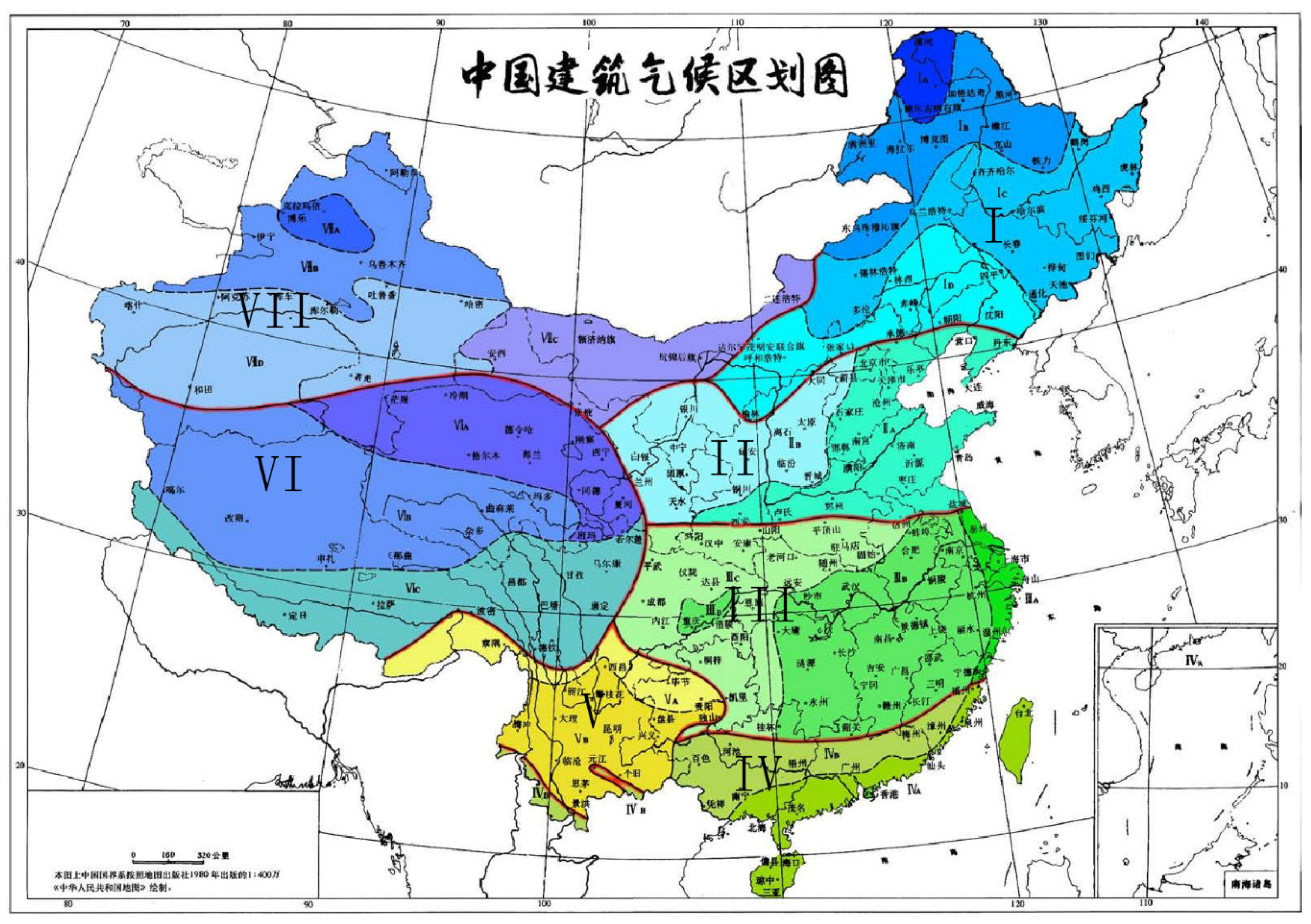
In this study, we apply the Standard of Climatic Zone Partition of China, which is a typical partition method used by Chinese architects for the purpose of distinguishing construction standards among regions with different climate characteristics.
As is displayed in
Figure 1, the standard divides the mainland of China into seven climatic zones according to the climatic patterns of different regions. We are more interested in the three coastal Climatic Zones I, II and III, as they constitute the eastern part of China, which is more economically developed and having a higher chance of issuing weather derivative contracts.
Eleven representative cities are selected, which cover Harbin and Changchun from Climatic Zone I; Beijing, Shijiazhuang, Ji’nan and Zhengzhou from Climatic Zone II; Nanjing, Hefei, Wuhan, Hangzhou and Nanchang from Climatic Zone III. Apart from the national capital Beijing, the rest of the representative cities in this study are chosen as they are the capital cities of the ten most agricultural productive provinces. This approach ensures that the locations of representative cities are distributed evenly and that the results are relevant for the highest possible number of inhabitants.
In order to calculate GDD indices and option prices, thirty years (from January 1984 to December 2013) of daily average temperature data collected from the China Meteorological Data Sharing Service System are used. Additionally, twenty-four years (from January 1984 to December 2007) of annual yield data collected from the China Agricultural Data Sharing System are used to conduct the efficiency tests. Note that we apply the yield data rather than the production data, as production also depends on the crop acreage, which changes from year to year.
3. Methodology
In order to test the efficiency of climatic zone-based GDD contracts for Chinese farmers, two questions need to be answered beforehand. First, a modeling method must be selected to evaluate temperature index contracts. The second question is whether climatic zone-based contracts are theoretically and practically appropriate. This section aims to give answers to both questions. Further, we provide a brief review of the continuous-autoregressive (CAR) model (Benth et al., 2007 [
9]) and present a method to determine the optimal tick size for temperature-based contracts. Finally, we explain the three test criteria of the efficiency tests.
3.1. Temperature Modeling and Derivative Pricing
There is a broad range of studies that is dedicated to researching an accurate approach for modeling temperature-based derivatives. One of the earliest methods is the burn analysis, which calculates the price relying on historical payoff data. Dornier and Queruel (2000) [
10] used for the first time a continuous-time Ornstein-Uhlenbeck (OU) process to model the temperature evolution. The OU process allows the simulation of the mean reverting random walk of the temperature dynamics. The first application of a stochastic model to real temperature data was presented by Alaton et al. (2002) [
11]. In order to calibrate the model to daily temperature, Alaton et al. (2002) [
11] included a sine function in the OU process. The temperature volatility is assumed to be monthly constant. Based on Alaton et al.’s study (2002) [
11], Benth et al. (2007) [
9] employed a continuous-autoregressive (CAR) process to fit the temperature evolution. Further, Benth et al. (2007) [
9] modeled the temperature volatility with truncated Fourier series, which enables functional modeling of the volatility process. In addition to stochastic temperature models, Schiller et al. (2012) [
12] introduced a spline model and applied it to daily temperature data of the USA.
In this study, the CAR model (Benth et al., 2007 [
9]) is applied to fit the temperature oscillations, as it is shown to be more suitable to model Chinese temperature data, in comparison with other existing temperature models (Zong and Ender, 2014 [
13], and Zong and Ender, 2016 [
14]). To give details, the CAR model models the temperature dynamics as the summation of a seasonal function and a CAR process. To be specific, temperature on day
can be expressed as:
is the function that captures the seasonal trend of the temperature process. It follows:
where
denotes the starting value of the sine function,
denotes the rate of global warming and
and
are respectively the scale parameter and the translation parameter of the sine function.
According to Benth et al. (2007) [
9],
expresses the
coordinate of the vector
, which is a vectorial OU process. Thus, the explicit solution of
in
for
follows:
where
and
,
is the
unit vector in
and
denotes the Brownian motion. The parameter
A is the mean-reverting
matrix given by:
where
are assumed to be constants. According to Benth et al. (2007) [
9], the optimal order
of the CAR process equals three.
Further, Benth et al. (2007) [
9] modeled the volatility
with a truncated Fourier series, which is expressed as:
where
are the parameters of the fourth ordered truncated Fourier series.
In order to estimate the model parameters, namely, in Equation (2), in Equation (4) and in Equation (5), we implement the regression using the ordinary least square method.
Hence, given the threshold temperature
and contract period
, the price of a GDD future contract at time
approximately follows (Benth et al., 2007 [
9]):
where:
Note that is the cumulative distribution function of a standard normal distribution.
Consequently, the price of a GDD option contract with strike price
K can be obtained from the following formula:
3.2. Climatic Zone-Based GDD Contracts
Weather derivatives can eliminate adverse selection and moral hazard as the valuation of their payoffs is based on an objective weather-index, which is impossible to manipulate. However, there is another type of risk that is inherent in weather derivatives: geographical basis risk should be considered with care. Practically, it is unlikely and extremely costly to cover all regions when weather derivatives are issued. In reality, weather contracts are written on weather indices of one specific location where the transaction takes place. Therefore, for those investors who are away from the trading spot, it is inevitable to be exposed to basis risk if they simply purchase weather contracts from the trading spot. According to the literature, there are at least two solutions for this problem. The first approach is to hedge basis risk via basis derivatives (Brockett et al., 2007 [
15]). This means that the investor buys a second option based on the observed differences of the weather index between the location of interest and the trading spot. However, from the buyers’ point of view, transaction costs might be high to purchase a second derivative when the market is already illiquid. The second approach is to add risk premiums that reflect geographical basis risk. This approach is proposed by Härdle and Osipenko (2012) [
16], who conducted an empirical analysis of temperature and price data from nine European cities. However, this method cannot be adopted for China as there are no real market data that allow the computation of the market price of risk. Woodard and Garcia (2008) [
17] compared the basis risk of weather contracts on the individual level and on the spatially-aggregated level, using the root mean squared loss (RMSL) and the expected shortfall (ES). Further, Okhrin et al. (2013) [
18] investigated the risk pooling efficiency of GDD contracts with buffer loads. Both studies indicated that spatial aggregation can reduce basis risk embedded in weather derivative contracts. Therefore, climatic zone-based contracts should theoretically prevail over city-based contracts in terms of basis risk, because it involves a greater level of aggregation. Albeit that mixed-indices contracts are suggested in the literature (Vedenov and Barnett, 2004 [
19]), the hedging power of such contracts is revealed to be lower in comparison to combinations of several simple index contracts (Pelka and Musshoff, 2013 [
20]).
Different from Woodard and Garcia (2008) [
17] and Okhrin et al. (2013) [
18], we compare climatic zone-based GDD contracts with city-based GDD contracts in terms of risk hedging efficiency. To begin with, we select a certain number of representative cities that are distributed evenly in the climatic zone. We assume that given the optimal growing temperature of a crop,
, the temperature deviations above and below
have the same effects on crop growth. Therefore, given the contract period [
], the GDD index of representative city
i and crop
j is expressed as:
where
is the daily observed temperatureand
denotes the optimal growing temperature of crop
j. Note that in our empirical tests, we proposed a so-called correlation-adjusted GDD index, which considered three different forms of deviations from the optimal growth temperature, namely the absolute value, the positive skewness and the negative skewness. The GDD of a given city was defined by the type of deviation that maximized the correlation between the corresponding index and the city’s crop yield. Efficiency tests were conducted based on the correlation-adjusted GDD. We found that it hardly provided a higher level of risk-reducing efficiency when the positive and negative skewness were considered. Therefore, we employed the absolute value of the deviations from the optimal growth temperature as the underlying GDD index in this paper.
Let the average climatic zone-based (ACZB) GDD index be equal to the average value of the GDD indices of the
representative cities in one climatic zone. Thus, the ACZB GDD of crop
j is given by:
Different from the averaged GDD, the weighted climatic zone-based (WCZB) GDD weights the individual GDD indices of the
representative cities by their crop yields, which follows:
where
is the proportion of the crop
yield of representative city
i over the total yield of all of the representative cities in the climatic zone. Hence, we have:
where
denotes the yield of crop
j in city
i during the contract period. The other two methods of calculating weights, respectively obtained from crop acreage and the maximized correlation between the climatic zone-based index and the total crop yield, were applied and tested empirically. From the results, we found that both of them failed to provide better results in terms of efficiency and stability, compared to the way we defined weights in this paper.
3.3. GDD Contract Optimization
In this part, we propose a method to determine the optimal tick size for GDD contracts under the framework of Vedenov and Barnett’s work (2004) [
19]. An optimized tick size is a crucial factor in terms of contract design and contributes directly to the risk hedging power of the contract. The overall idea of the optimization is to find a coefficient
that minimizes the aggregated semi-variance of the loss (Markowitz, 1991 [
21]; Vedenov and Barnett, 2004 [
19]).
By first assuming that the annual yield series attains an exponential growth, the annual yield
can be written as:
where
is the white noise; and
is the linear time trending the logarithm of the annual yield
, which is given by:
Thus, the annual time-detrended yield
can be obtained by:
where
denotes the initial time.
Therefore, the optimal tick size
of a GDD contract can be solved by minimizing the aggregated semi-variance of the loss:
where
is the option price under the CAR model (Benth et al., 2007) [
9],
is the corresponding payoff and
denotes the long-term average yield of a crop.
3.4. Efficiency Comparison
In order to compare the efficiency of city-based and the climatic zone-based GDD contracts in terms of risk reduction for farm households, we analyze the annual revenues of a certain crop with and without the considered GDD contracts. In the case of city-based contracts, we consider two scenarios. The first one (Case 1) is an ideal situation where weather contract transactions take place in all of the representative cities, while the second situation (Case 2) is more practical, which allows only one trading spot in each climatic zone. In Case 2, the trading spots are Changchun (Climatic Zone I), Shijiazhuang (Climatic Zone II) and Hefei (Climatic Zone III). The trading spots are selected, because they are located in the center of the other representative cities in their climatic zone.
Note that in this study, only European option contracts are considered. According to Vedenov and Barnett (2004) [
19], the revenue without the GDD contract equals the gross income of selling the commodity, which follows:
while the revenue with the GDD contract is given by:
where
p is the commodity price of the corresponding crop and
is the time-detrended yield. The reason why
is applied to calculate the revenue is that it eliminates any time-related trends in the time series of yield data; thus ideally, weather is the only factor that causes yield changes.
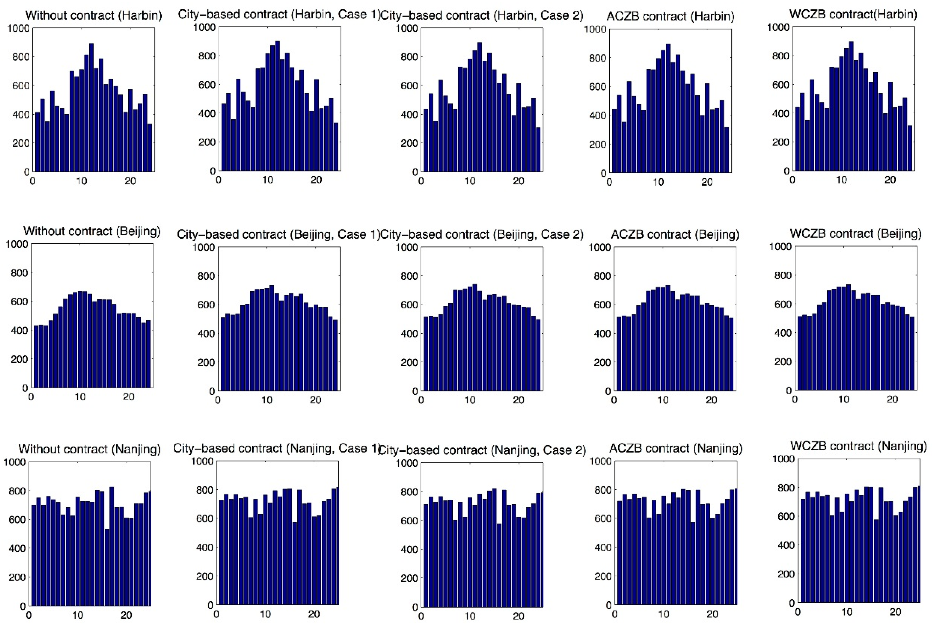
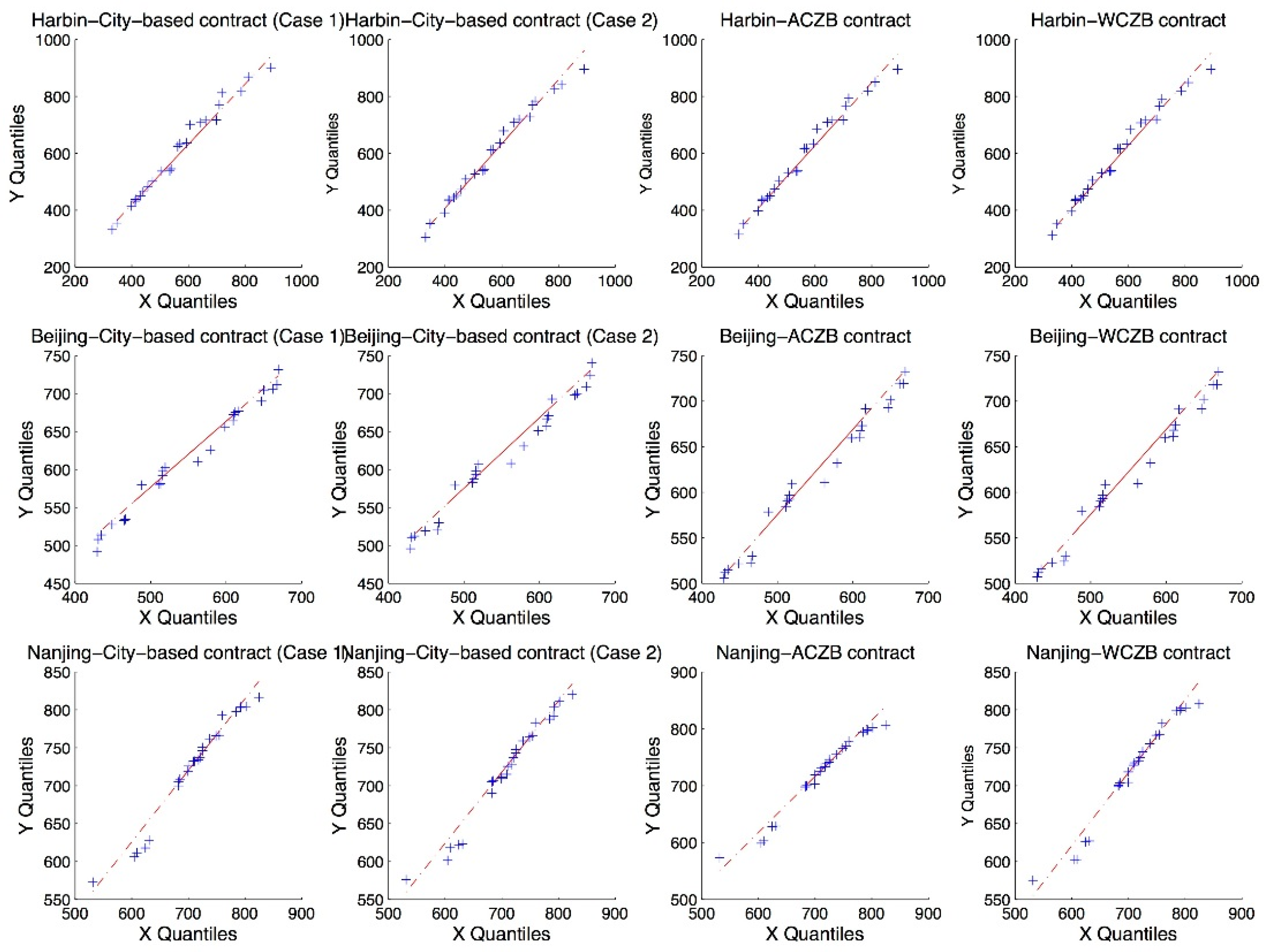
We start off with comparing revenue distributions with and without GDD contracts. Histograms, quantile-quantile (Q-Q) plots and Kolmogorov-Smirnov tests are employed in our study to analyze the revenue distributions. Note that in the case of climatic zone-based contracts, the yield in Equations (20) and (21) stays at the city level, as the objective is to compare the hedging power towards local weather risks.
Next, we apply three test criteria used by Vedenov and Barnett (2004) [
19] in order to gain implications on the efficiency of weather contracts. Let
denote the distribution of the revenue. The definitions and the mathematical expressions of the test criteria are given below:
The mean root square loss (MRSL):
The certainty-equivalent revenues (CERs):
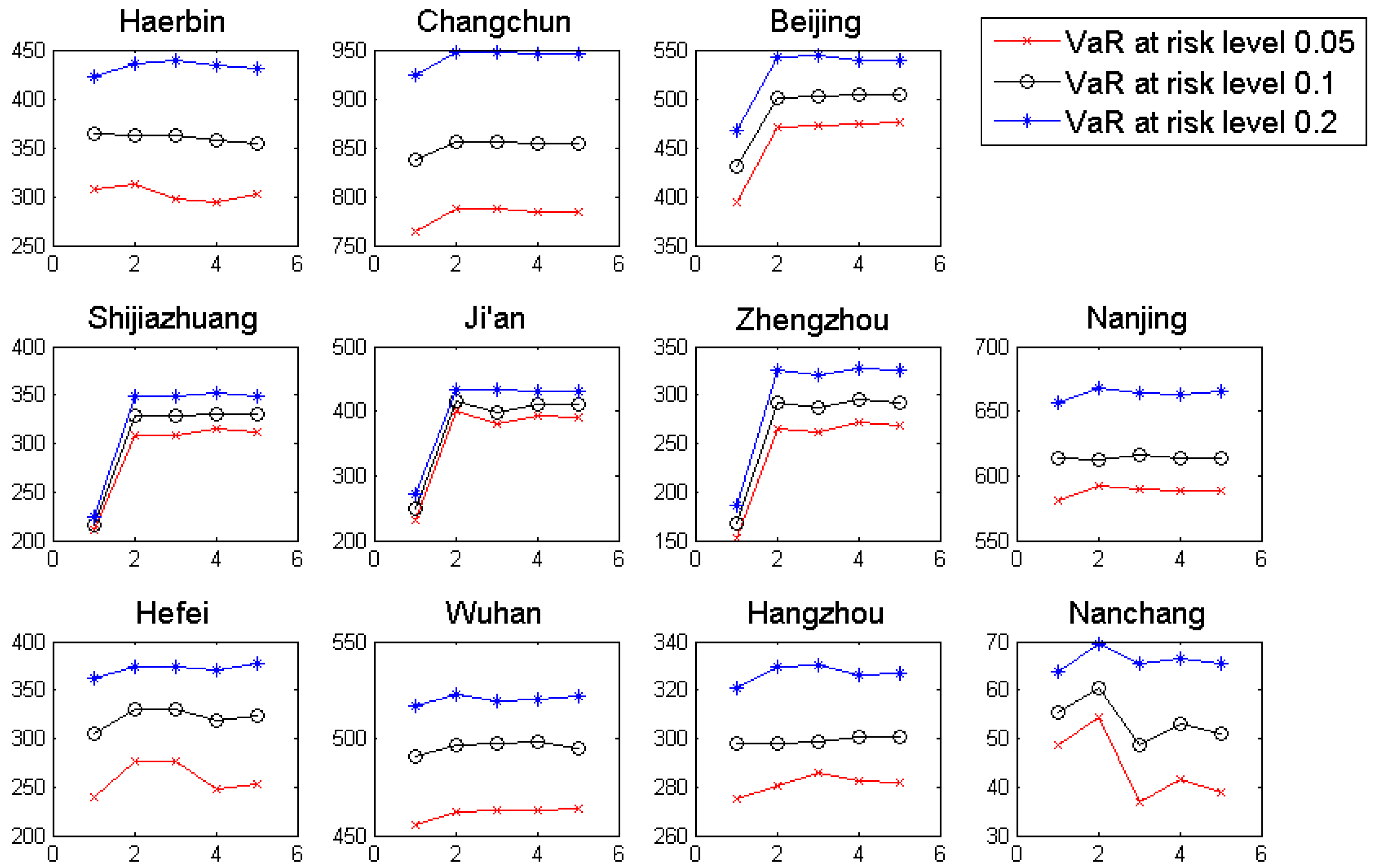
The first criterion, the MRSL, measures the semi-variance of the revenue distribution. A smaller MRSL indicates a lower level of revenue variation, thus less pronounced yield risks. The VaR is an inverse function of the cumulative density function of the return distribution, which measures the value of return at a given risk level and over a defined time horizon. By computing the VaR for different confidence levels , one can gain a general understanding of the return distribution. Last, the CERs compute expected revenues with a given level of risk aversion. Both the VaR and the CERs assess the risk hedging power of a weather contract in a different way than MRSL. For VaR and CERs a smaller value refers to a lower degree of risk exposure.
Note that in the case of CERs, we estimate the risk aversion level
(Babcock et al., 1993 [
22]) by the following equation:
We compute the value of in Equation (24) with different risk premiums , i.e., 0%, 5% and 10%. However, we find that for yield data of Chinese cities, the results across cities and risk premiums exclusively tend to 1. This result indicates an extremely high level of risk aversion of Chinese farm households, which agrees with the literature. Under this condition, the values of the CERs of a given city should be proportional to the corresponding values of the risk premiums.
5. Conclusions
In this paper, we introduce two climatic zone-based indices for temperature-based derivative contracts, i.e., the ACZB GDD and the WCZB GDD contracts. The objectives are to reduce the model dimension of temperature-based derivative pricing in China and to analyze the risk hedging power of climatic zone-based contracts for Chinese farm households.
In addition to Ender and Zhang’s (2015) [
3] and Sun et al.’s (2014) [
5] studies, which both confirm that city-based temperature indices are efficient hedging tools against yield-variation risks, we conclude that both climatic zone-based GDD contracts and city-based GDD contracts manage to reduce risks related to crop productivity in this study. In terms of cross-regional temperature-based derivatives modeling, this study suggests the possibility of contract spatial aggregation without influencing its risk hedging power, which is basically in line with Göncü and Zong’s study (2013) [
8]. With respect to the results, changes of the GDD distributions are observed after transforming city-based GDD indices into climatic zone-based GDD indices. Regarding the results of efficiency tests, we infer that climatic zone-based GDD contracts have the same power to reduce fluctuations of the farmers’ income as city-based contracts. In some cases as for MRSLs and CERs, climatic zone-based GDD contracts even dominate. For the VaRs, the performances of climatic zone-based and city-based contracts are alike, with half of the cities having higher VaRs in each case. Furthermore, the average GDD and the weighted GDD generate similar contract prices on climatic zone levels, which leads to similar effects on risk reduction.
In the practical application, our study suggests that deliberately-used climatic zone-based GDD contracts can be a more efficient instrument for agricultural risk management due to the feature of cost reduction. Specifically, the ACZB GDD index is recommended as more suitable for agricultural risk management in China. By launching derivative contracts written on the ACZB GDD index, cities in the same climatic zone can use a common contract, which shares a unique price, to achieve the purpose of hedging weather risks. Such a means of transaction increases the efficiency, both in terms of modeling and market management. Additionally, no crop yield data are required to calculate ACZB indices, which is different from WCZB indices. Thus, the pricing procedure is simplified.
For future research, we intend to perform a study focused on GDD distributions. As the CAR model (Benth et al., 2007) [
9] prices temperature-based derivatives with the assumption that the underlying indices are normally distributed, we assume that with a deeper understanding of the GDD distributions, more precise models for Chinese climatic zone-based GDD contracts can be derived. Additionally, a weather-yield regression model is recommended to be deduced and applied in order to conduct out-of-sample efficiency tests.


