Petroleum Hydrocarbon Profiles of Water and Sediment of Algoa Bay, Eastern Cape, South Africa


Abstract
: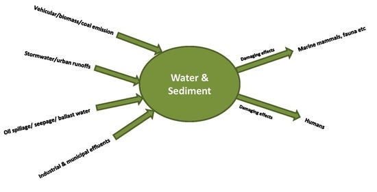
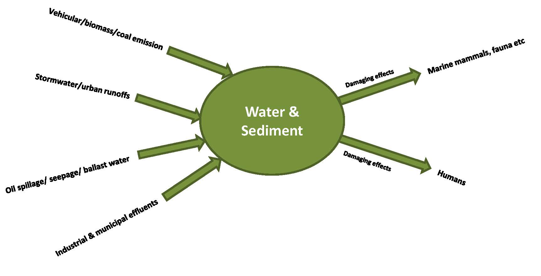
1. Introduction
2. Materials and Methods
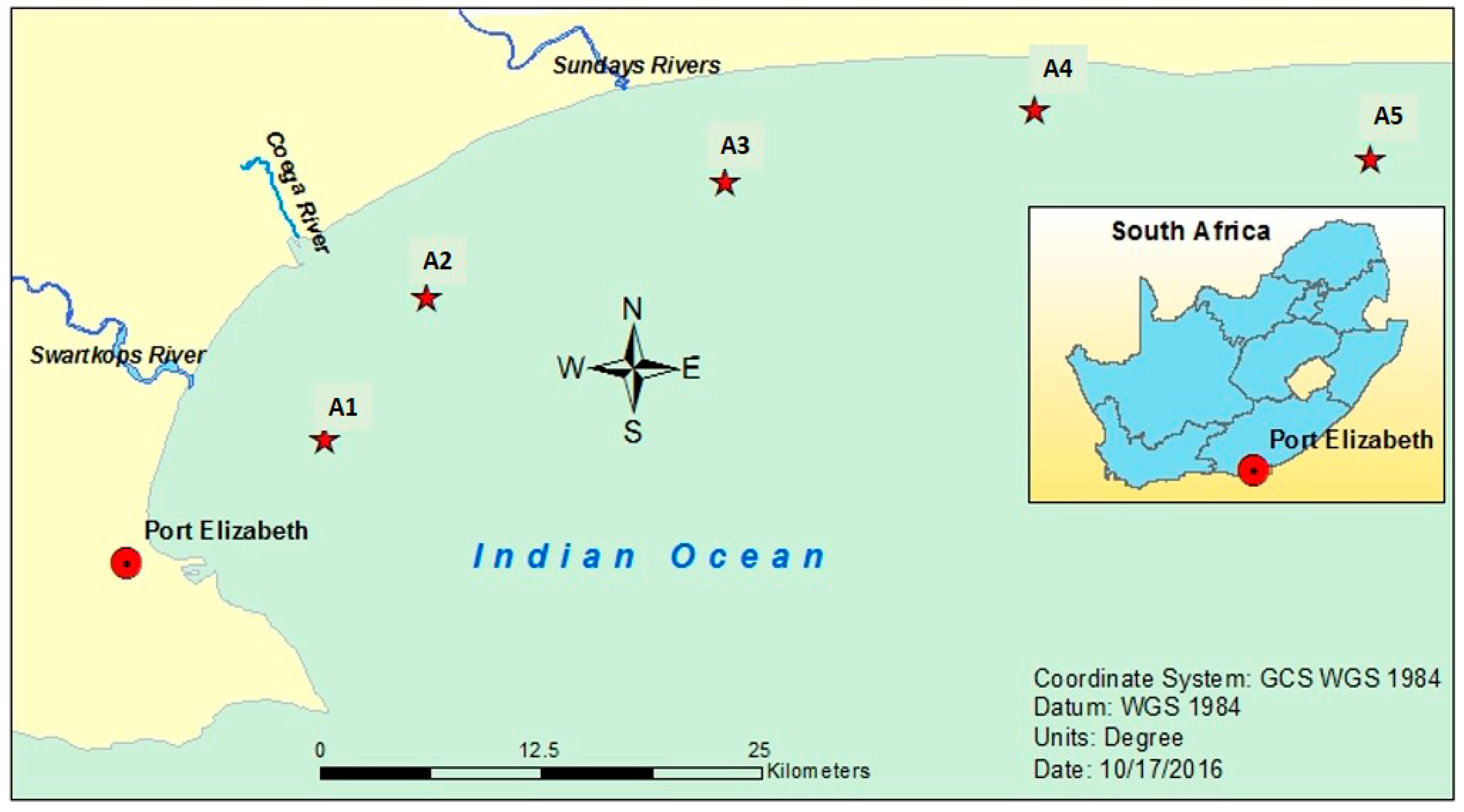
2.1. Study Area
2.2. Chemicals and Sample Collection
2.3. Physicochemical Analyses of the Samples
2.4. Extraction of Petroleum Hydrocarbon from Water and Sediment Samples
2.5. Silica Gel Cleanup and Separation
2.6. Gas Chromatography Analysis and Quantitation
2.7. Quality Control
2.8. Data Analysis
3. Results and Discussion
3.1. Physicochemical Properties of the Surface and Bottom Water of Algoa Bay
3.2. Total Petroleum Hydrocarbon Levels in the Waters
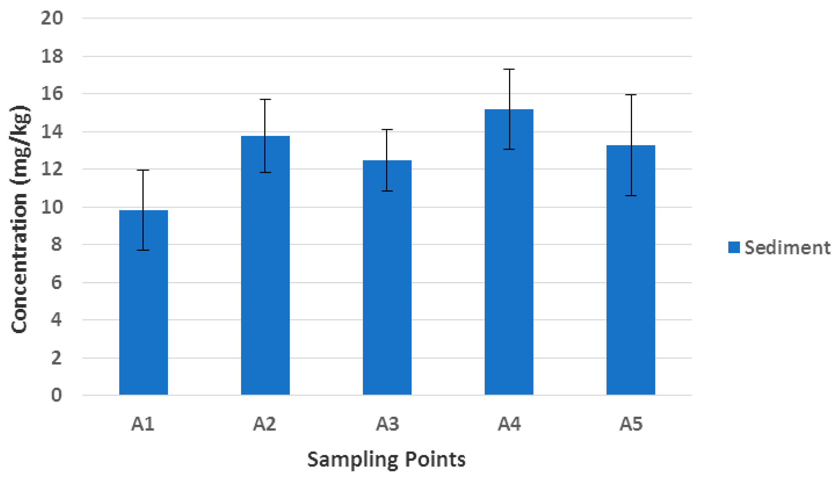
3.3. Total Petroleum Hydrocarbon Levels in the Sediment Samples
3.4. Organic Carbon Content of the Sediment
3.5. Concentrations of n-Alkanes and Source Identification
3.5.1. Carbon Preference Index (CPI)
3.5.2. UCM and Weathering Index (WI)
3.5.3. Low Molecular Weight n-Alkanes/High Molecular Weights Alkanes (L/H)
3.5.4. C31/C19
3.5.5. Long Chain Hydrocarbons/Short Chain Hydrocarbons (LHC/SHC)
3.5.6. Average Carbon Length (ACL)
4. Conclusions
Acknowledgments
Author Contributions
Conflicts of Interest
References
- Wu, Y.; Zhang, J.; Mi, T.Z.; Li, B. Occurrence of n-alkanes and polycyclic aromatic hydrocarbons in the core sediments of the Yellow sea. Mar. Chem. 2001, 76, 1–15. [Google Scholar] [CrossRef]
- Muthukumar, A.; Idayachandiran, G.; Kumaresan, S.; Kumar, T.A.; Balasubramanian, T. Petroleum hydrocarbons (PHC) in sediments of three different ecosystems from Southeast Coast of India. Int. J. Pharm. Biol. Arch. 2013, 4, 543–549. [Google Scholar]
- Quevenco, R. Sustainable Growth of Coastal Waters: A profile of the history and levels of coastal pollution in the Caribbean emerges. IAEA Bull. 2011, 53-1, 32–37. [Google Scholar]
- River Health Programme (RHP). State-of-Rivers Report: Buffalo River System; Department of Water Affairs and Forestry: Pretoria, South Africa, 2004; pp. 17–33.
- Commendatore, M.G.; Esteves, J.L. Natural and anthropogenic hydrocarbons in sediments from the Chubut River (Patagonia, Argentina). Mar. Poll. Bull. 2004, 48, 910–918. [Google Scholar] [CrossRef] [PubMed]
- Agency for Toxic Substances and Disease Registry (ATSDR). Toxicological Profile for Total Petroleum Hydrocarbon; Department of Health and Human Services, Public Health Service: Atlanta, GA, USA, 1999; pp. 9–37.
- Gao, X.; Chen, S.; Xie, X.; Long, A.; Ma, F. Non-aromatic hydrocarbons in surface sediments near the Pearl River estuary in the South China Sea. Environ. Pollut. 2007, 148, 40–47. [Google Scholar] [CrossRef] [PubMed]
- Zrafi, I.; Hizem, L.; Chalghmi, H.; Ghrabi, A.; Rouabhia, M.; Saidane-Mosbahi, D. Aliphatic and aromatic biomarkers for petroleum hydrocarbon investigation in marine sediment. J. Pet. Sci. Res. 2013, 2, 145–155. [Google Scholar] [CrossRef]
- Rayner, J.L.; Snape, I.; Walworth, J.L.; Harvey, P.M.; Ferguson, S.H. Petroleum–hydrocarbon contamination and remediation by microbioventing at sub-Antarctic Macquarie Island. Cold Reg. Sci. Technol. 2007, 48, 139–153. [Google Scholar] [CrossRef]
- Ahmed, O.E.; Ali, N.A.; Mahmoud, S.A.; Doheim, M.M. Environmental assessment of contamination by petroleum hydrocarbons in the aquatic species of Suez Gulf. Int. J. Mod. Org. Chem. 2014, 3, 1–17. [Google Scholar]
- Hatje, V.; Payne, T.E.; Hill, D.M.; Mcorist, G.; Birch, G.F.; Szymczak, R. Kinetics of trace element uptake and release by particles in estuarine waters: Effects of pH, salinity, and particle loading. Environ. Int. 2003, 29, 619–629. [Google Scholar] [CrossRef]
- Olver, C. Report on Issues Relating to the Potential Relocation of the Port Elizabeth Manganese Terminal and Tank Farm to the Port of Ngqura; Compiled for the Port Elizabeth Regional Chamber of Commerce: Port Elizabeth, South Africa, 2008; pp. 2–55. [Google Scholar]
- Farrington, J.W.; Takada, H. Persistent organic pollutants (POPs), polycyclic aromatic hydrocarbons (PAHs), and plastics: Examples of the status, trend, and cycling of organic chemicals of environmental concern in the ocean. Oceanography 2014, 27, 196–213. [Google Scholar] [CrossRef]
- Ali, S.A.M.; Payus, C.; Ali, M.M. Surface sediment analysis on petroleum hydrocarbon and total organic carbon from coastal area of Papar to Tuaran, Sabah. Malays. J. Anal. Sci. 2015, 19, 318–324. [Google Scholar]
- Adeniji, A.O.; Okoh, O.O.; Okoh, A.I. Analytical methods for the determination of the distribution of total petroleum hydrocarbons in the water and sediment of aquatic systems: A review. J. Chem. 2017, 5178937. [Google Scholar] [CrossRef]
- Harji, R.R.; Yvenat, A.; Bhosle, N.B. Sources of hydrocarbons in sediments of the Mandovi Estuary and the Marmugoa Harbour, West Coast of India. Environ. Int. 2008, 34, 959–965. [Google Scholar] [CrossRef] [PubMed]
- Kumar, V.; Arya, S.; Dhaka, A.; Minakshi; Chanchal. A study on physico-chemical charactersitics of Yamuna River around Hamirpur (UP), Bundelkhand Region Central India. Int. Multidiscip. Res. J. 2011, 1, 14–16. [Google Scholar]
- Mustapha, M.K.; Omotosho, J.S. An assessment of the physico-chemical properties of Moro Lake, Kwara State, Nigeria. Afr. J. Appl. Zool. Environ. Biol. 2005, 7, 3–77. [Google Scholar]
- Sangpal, R.R.; Kulkarni, U.D.; Nandurkar, Y.M. An assessment of the physico-chemical properties to study the pollution potential of Ujjani Reservoir, Solapur District, India. ARPN J. Agric. Biol. Sci. 2011, 6, 34–38. [Google Scholar]
- El-Amier, Y.A.; Zahran, M.A.; Al-Mamory, S.H. Assessment the physico-chemical characteristics of water and sediment in Rosetta Branch, Egypt. J. Water Resour. Prot. 2015, 7, 1075–1086. [Google Scholar] [CrossRef]
- Sharma, A.; Sharma, R.C.; Anthwal, A. Monitoring phytoplankton diversity in the hill stream Chandrabhaga in Garhwal Himalayas. Life Sci. J. 2007, 4, 80–84. [Google Scholar]
- Yadav, R.C.; Srivastava, V.C. Physicochemical properties of the water of River Ganga at Ghazipur. Indian J. Sci. Res. 2011, 2, 41–44. [Google Scholar]
- Chigor, V.N.; Sibanda, T.; Okoh, A.I. Variations in the physicochemical characteristics of the Buffalo River in the Eastern Cape Province of South Africa. Environ. Monit. Assess. 2013, 185, 8733–8747. [Google Scholar] [CrossRef] [PubMed]
- Gebreyohannes, F.; Gebrekidan, A.; Hadera, A.; Estifanos, S. Investigations of physico-chemical parameters and its pollution implications of Elala River, Mekelle, Tigray, Ethiopia. Momona Ethiop. J. Sci. 2015, 7, 240–257. [Google Scholar] [CrossRef]
- Cortes, J.E.; Suspes, A.; Roa, S.; González, C.; Castro, H.E. Total petroleum hydrocarbons by gas chromatography in Colombian waters and soils. Am. J. Environ. Sci. 2012, 8, 396–402. [Google Scholar]
- Sharma, R.C.; Singh, N.; Chauhan, A. The influence of physico-chemical parameters on phytoplankton distribution in a head water stream of Garhwal Himalayas: A case study. Egypt. J. Aquat. Res. 2016, 42, 11–21. [Google Scholar] [CrossRef]
- Okoh, A.I.; Odjadjare, E.E.; Igbinosa, E.O.; Osode, A.N. Wastewater treatment plants as a source of microbial pathogens in the receiving watershed. Afr. J. Biotechnol. 2007, 6, 2932–2944. [Google Scholar]
- Mason, R.P. Hydrocarbons in mussels around the Cape Peninsula, South Africa. S. Afr. J. Mar. Sci. 1988, 7, 139–151. [Google Scholar] [CrossRef]
- Okonkwo, J.O.; Awofolu, O.R.; Moja, S.J.; Forbes, P.C.B.; Senwo, Z.N. Total petroleum hydrocarbons and trace metals in street dusts from Tshwane Metropolitan Area, South Africa. J. Environ. Sci. Health Part A 2006, 41, 2789–2798. [Google Scholar] [CrossRef] [PubMed]
- Adeniji, A.O.; Okoh, O.O.; Okoh, A.I. Petroleum hydrocarbon fingerprints of water and sediment samples of Buffalo River estuary in the Eastern Cape Province, South Africa. J. Anal. Methods Chem. 2017, 2629365. [Google Scholar] [CrossRef] [PubMed]
- Klages, N.; Jegels, J.; Schovell, I.; Vosloo, M. Nelson Mandela Bay Municipality State of Environment Report; Nelson Mandela Bay Municipality: Port Elizabeth, South Africa, 2011; pp. 24–118. [Google Scholar]
- Klages, N.T.W.; Bornman, T.G. Port of Ngqura marine biomonitoring programme. Winter 2005. Inst. Environ. Coast. Manag. 2005, C28, 30–31. [Google Scholar]
- Klages, N.T.W.; Bornman, T.G. Port of Ngqura Marine Biomonitoring Programme. Annual Report 2002–2003; Institute for Environmental and Coastal Management, 2003; Volume C86, p. 66. [Google Scholar]
- Pichegru, L.; Grémillet, D.; Crawford, R.J.M.; Ryan, P.G. Marine no-take zone rapidly benefits endangered penguin. Biol. Lett. 2010, 6, 498–501. [Google Scholar] [CrossRef] [PubMed]
- Council for Scientific and Industrial Research (CSIR). Chapter 6: Marine Ecology, Sediment Toxicology and Dredging. In Proposed Extension to the Container Berth and Construction of an Administration Craft Basin at the Port of Ngqura; Draft Scoping Report; CSIR: Stellenbosch, South Africa, 2007; pp. 8–18. [Google Scholar]
- Sustainable Seas Trust (SST). Algoa Bay Conservation. Available online: http://www.sst.org.za/hope-spots/algoa-bay-hope-spot--2/algoa-bay-hope-spot-details (accessed on 6 December 2016).
- Hilmer, T.; Bate, G.C. Hydrocarbon levels in the Swartkops Estuary: A preliminary study. Water SA 1987, 13, 180–183. [Google Scholar]
- Bornman, T.G. Report on seawater quality in the port of Port Elizabeth (March 2003). Inst. Environ. Coast. Manag. 2003, C82, 26. [Google Scholar]
- Coastal and Environmental Services (CES). The Subsequent Environmental Impact Report for the Proposed Port of Ngqura; Coastal and Environmental Services: Grahmstown, South Africa, 2001. [Google Scholar]
- African Environmental Solutions (AES). Algoa Bay Management Plan. Prepared by CLABBS Consortium; African Environmental Solutions: Kenilworth, South Africa, 1999; p. 63. [Google Scholar]
- Enviro-Fish Africa. C.A.P.E. Estuaries Management Programme; Swartkops Integrated Environmental Management Plan: Draft Situation Assessment, 1st Draft; Enviro-Fish Africa: Grahamstown, South Africa, 2009. [Google Scholar]
- Klages, N.T.W.; Paterson, A.; Sauer, W.; Shipton, T.; Vromans, D. Towards a coastal management plan for the Nelson Mandela Metropolitan Municipality: A starter document. Inst. Environ. Coast. Manag. 2003, 42, 1–164. [Google Scholar]
- Griffiths, B.; Bassa, H. Municipal Solid Waste Diversion and Beneficiation Opportunities at Nelson Mandela Bay Metro Municipality, Feasibility Study Final Report; Royal HaskoningDHV: Buffalo City-East London, South Africa, 2014; pp. 183–184. [Google Scholar]
- Ryan, P.G.; Bouwman, H.; Moloney, C.L.; Yuyama, M.; Takada, H. Long-term decreases in persistent organic pollutants in South African coastal waters detected from beached polyethylene pellets. Mar. Pollut. Bull. 2012, 64, 2756–2760. [Google Scholar] [CrossRef] [PubMed]
- Olajire, A.A.; Alade, A.O.; Adeniyi, A.A.; Olabemiwo, O.M. Distribution of polycyclic aromatic hydrocarbons in surface soils and water from the vicinity of Agbabu bitumen field of Southwestern Nigeria. J. Environ. Sci. Health Part A 2007, 42, 1043–1049. [Google Scholar] [CrossRef] [PubMed]
- Badina, A.; Faureb, P.; Bedella, J.; Delolmea, C. Distribution of organic pollutants and natural organic matter in urban storm water sediments as a function of grain size. Sci. Total Environ. 2008, 403, 178–187. [Google Scholar] [CrossRef] [PubMed]
- Motsara, M.R.; Roy, R.N. Guide to laboratory establishment for plant nutrient analysis. FAO Fertil. Plant Nutr. Bull. 2008, 19, 38–42. [Google Scholar]
- Laboratory Analytical Work Instruction. Laboratory Analytical Work Instruction (LAWI) for the Determination of Total Petroleum Hydrocarbon in Soil/Sediment/Sludge in Gas Chromatography; Fugro (Nig.) Ltd.: Lagos, Nigeria, 2011; p. 9. [Google Scholar]
- Alinnor, I.J.; Ogukwe, C.E.; Nwagbo, N.C. Characteristic level of total petroleum hydrocarbon in soil and groundwater of oil impacted area in the Niger Delta region, Nigeria. J. Environ. Earth Sci. 2014, 4, 188–194. [Google Scholar]
- Sakari, M.; Ting, L.S.; Houng, L.Y.; Lim, S.K.; Tahir, R.; Adnan, F.A.F.; Yi, A.L.J.; Soon, Z.Y.; Hsia, B.S.; Shah, M.D. Urban effluent discharge into rivers: A forensic chemistry approach to evaluate the environmental deterioration. World Appl. Sci. J. 2012, 20, 1227–1235. [Google Scholar]
- Maioli, O.L.G.; Rodrigues, K.C.; Knoppers, B.A.; Azevedo, D.A. Distribution and sources of aliphatic and polycyclic aromatic hydrocarbons in suspended particulate matter in water from two Brazilian estuarine systems. Cont. Shelf Res. 2011, 31, 1116–1127. [Google Scholar] [CrossRef]
- Sakari, M.; Zakaria, M.P.; Junos, M.; Anuar, N.A.; Yun, H.Y.; Heng, Y.S.; Zainuddin, M.H.; Chai, K.L. Spatial distribution of petroleum hydrocarbon in sediments of major rivers from east coast of Peninsular Malaysia. Coast. Mar. Sci. 2008, 32, 1–10. [Google Scholar]
- Charriau, A.; Bodineau, L.; Ouddane, B.; Fischer, J. Polycyclic aromatic hydrocarbons and n-alkanes in sediments of the Upper Scheldt River Basin: contamination levels and source apportionment. J. Environ. Monit. R. Soc. Chem. 2009, 11, 1086–1093. [Google Scholar] [CrossRef] [PubMed]
- Ahmed, O.E.; Mahmoud, S.A.; Mousa, A.E.M. Aliphatic and poly-aromatic hydrocarbons pollution at the drainage basin of Suez Oil Refinery Company. Curr. Sci. Int. 2015, 4, 27–44. [Google Scholar]
- Luan, W.; Szelewski, M. Ultra-fast total petroleum hydrocarbons (TPH) analysis with agilent low thermal mass (LTM) GC and simultaneous dual-tower injection. In Agilent Technologies Application Note; Agilent: Santa Clara, CA, USA, 2008; pp. 1–8. [Google Scholar]
- Caruso, A.; Santoro, M. Detection of Organochlorine Pesticides by GC-ECD Following U.S. EPA Method 8081; Thermo Fisher Scientific Inc.: Milan, Italy, 2014; pp. 1–4. [Google Scholar]
- Nekhavhambe, T.J.; Van Ree, T.; Fatoki, O.S. Determination and distribution of polycyclic aromatic hydrocarbons in rivers, surface runoff, and sediments in and around Thohoyandou, Limpopo Province, South Africa. Water SA 2014, 40, 415–425. [Google Scholar] [CrossRef]
- Kansas Department of Health and Environment (KDHE). Kansas Method for the Determination of Mid-Range Hydrocarbons (MRH) and High-Range Hydrocarbons (HRH); Kansas Department of Health and Environment: Topeka, KS, USA, 2015; pp. 18–20. [Google Scholar]
- Texas Natural Resource Conservation Commission (TNRCC). Total Petroleum Hydrocarbons, TNRCC Method 1005, Revision 03; TNRCC: Austin, TX, USA, 2001; p. 26. [Google Scholar]
- Chapman, D. (Ed.) Water Quality Assessments—A Guide to Use of Biota, Sediments and Water in Environmental Monitoring, 2nd ed.; E&FN Spon: Great Britain, 1996; pp. 40–133. [Google Scholar]
- United Nations Environment Programme Global Environment Monitoring System/Water Programme (UNEPGEMS). Water Quality for Ecosystem and Human Health, 2nd ed.; UNEPGEMS: Nairobi, Kenya, 2008; pp. 3–31. [Google Scholar]
- Sorlini, S.; Palazzini, D.; Sieliechi, J.M.; Ngassoum, M.B. Assessment of physical-chemical drinking water quality in the Logone Valley (Chad-Cameroon). Sustainability 2013, 5, 3060–3076. [Google Scholar] [CrossRef]
- Australian and New Zealand Environment and Conservation Council (ANZECC). Aquatic Ecosystems—Rationale and Background Information (Paper No 4, Chapter 8): Australian and New Zealand Guidelines for Fresh and Marine Water Quality; ANZECC: Wellington, New Zealand, 2000; Volume 2, p. 678. [Google Scholar]
- Department of Environmental Affairs (DEA). Chapter 9: Oceans and Coasts: Ocean and Coasts Ecosystem Services Are Important as They Directly and Indirectly Impact on Human Livelihoods, Food Security and Agriculture; Oceans and Coasts: Pretoria, South Africa, 2012; p. 26. [Google Scholar]
- Gupta, N.; Yadav, K.K.; Kumar, V.; Singh, D. Assessment of physicochemical properties of Yamuna River in Agra City. Int. J. Chem. Technol. Res. 2013, 5, 528–531. [Google Scholar]
- Fondriest Environmental Inc. (FEI). Conductivity, Salinity and Total Dissolved Solids: Fundamentals of Environmental Measurements. 2014. Available online: http://www.fondriest.com/environmental-measurements/parameters/water-quality/conductivity-salinity-tds/ (accessed on 23 November 2016).
- Australian and New Zealand Environment and Conservation Council (ANZECC). The Guidelines (Paper No 4, Chapters 1–7): Australian and New Zealand Guidelines for Fresh and Marine Water Quality; ANZECC: Wellington, New Zealand, 2000; Volume 1, p. 314. [Google Scholar]
- Department of Environment and Conservation (DEC) NSW. Marine Water Quality Objectives for NSW Ocean Waters: Sydney Metropolitan and Hawkesbury—Nepean; DEC: Sydney, Australia, 2005; p. 28. [Google Scholar]
- Greene, K. Beach Nourishment: A Review of the Biological and Physical Impacts; ASMFC Habitat Management Series # 7; Atlantic States Marine Fisheries Commission: Arlington, VA, USA, 2002; p. 179. [Google Scholar]
- Environmental Protection Agency, Ireland (EPAI). Parameters of Water Quality: Interpretation and Standards; EPAI: Wexford, Ireland, 2001; pp. 25–119. [Google Scholar]
- Schumann, E.H. The coastal ocean off southeast Africa, including Madagascar. In the Global Coastal Ocean; John Wiley & Sons: New York, NY, USA, 1998; Volume 11, pp. 557–582. [Google Scholar]
- Goschen, W.S.; Schumann, E.H. The Physical Oceanographic Processes of Algoa Bay, With Emphasis on the Western Coastal Region; South African Environmental Observation Network (SAEON) & Institute for Maritime Technology (IMT): Pretoria, South Africa, 2011; p. 69. [Google Scholar]
- Department for International Development (DFID). A Simple Methodology for Water Quality Monitoring; Pearce, G.R., Chaudhry, M.R., Ghulum, S., Eds.; Department for International Development Wallingford: Chatham, UK, 1999; 16p. [Google Scholar]
- Fondriest Environmental Inc. (FEI). Dissolved Oxygen: Fundamentals of Environmental Measurements. 2013. Available online: http://www.fondriest.com/environmental-measurements/parameters/water-quality/dissolved-oxygen/ (accessed on 23 November 2016).
- Murphy, S. General Information on Dissolved Oxygen: Dissolved Oxygen. City of Boulder/USGS Water Quality Monitoring, 2007. Available online: http://bcn.boulder.co.us/basin/data/NEW/info/DO.html (accessed on 2 August 2017).
- Hoyer, M.V.; Frazer, T.K.; Notestein, S.K.; Canfield, D.E., Jr. Nutrient, chlorophyll, and water clarity relationships in Florida’s nearshore coastal waters with comparisons to freshwater lakes. Can. J. Fish. Aquat. Sci. 2002, 59, 1024–1031. [Google Scholar] [CrossRef]
- Suratman, S. Distribution of total petrogenic hydrocarbon in Dungun River Basin, Malaysia. Orient. J. Chem. 2013, 29, 77–80. [Google Scholar] [CrossRef]
- Lee, J. Endangered African Penguins under Threat Following Oil Spill. SABC News Feeds, 2016. Available online: http://www.sabc.co.za/news/a/b540c1004df610f685d3f546a0a81a58/Endangered-African-Penguins-under-threat-following-oil-spill-20160822 (accessed on 23 November 2016).
- Van Ballegooyen, R.C.; Schoeman, B. Dock Berth Deepening Project: Integrated Marine Impact Assessment Study; CSIR Report: Pretoria, South Africa, 2007. [Google Scholar]
- Wattayakorn, G.; Rungsupa, S. Petroleum hydrocarbon residues in the marine environment of Koh Sichang-Sriracha, Thailand. Coast. Mar. Sci. 2012, 35, 122–128. [Google Scholar]
- Li, Y.; Zhao, Y.; Peng, S.; Zhou, Q.; Ma, L.Q. Temporal and spatial trends of total petroleum hydrocarbons in the seawater of Bohai Bay, China from 1996 to 2005. Mar. Pollut. Bull. 2010, 60, 238–243. [Google Scholar] [CrossRef] [PubMed]
- Tiganus, D.; Coatu, V.; Lazar, L.; Oros, A. Present level of petroleum hydrocarbons in seawater associated with offshore exploration activities from the Romanian Black Sea sector. Cercetari Mar. 2016, 46, 98–108. [Google Scholar]
- Korshenko, A.; Matveichuk, I.; Plotnikova, T.; Luchkov, V. Marine Water Pollution, Annual Report 2003; Hydrometeoizdat: St. Petersburg, Russia, 2005. (In Russian) [Google Scholar]
- Morris, J.P. Residual Diesel Range Organics and Selected Frothers in Process Waters from Fine Coal Flotation. Master’s Thesis, Virginia Polytechnic Institute and State University, Blacksburg, VA, USA, 2013. [Google Scholar]
- Wongnapapan, P.; Wattayakorn, G.; Snidvongs, A. Petroleum hydrocarbon in seawater and some sediments of the South China Sea, Area I: Gulf of Thailand and East Coast of Peninsular Malaysia. In Proceedings of the 1st Technical Seminar on Marine Fishery Resources Survey in the South China Sea; Training Department, Southeast Asian Fisheries Development Center: Samut Prakan, Thailand, 1999; pp. 105–110. [Google Scholar]
- Maktoof, A.A.; Alkhafaji, B.Y.; Al-Janabi, Z.Z. Evaluation of total hydrocarbons levels and traces metals in water and sediment from main outfall drain in Al-Nassiriya City/Southern Iraq. Nat. Resour. 2014, 5, 795–803. [Google Scholar] [CrossRef]
- Karem, D.S.; Kadhim, H.A.; Al-Saad, H.T. Total Petroleum Hydrocarbons (TPH) in the Soil of West Qurna-2 Oil Field Southern Iraq. J. Chem. Pharm. Res. 2016, 9, 40–45. [Google Scholar]
- Khillare, P.S.; Hasan, A.; Sarkar, S. Accumulation and risks of polycyclic aromatic hydrocarbons and trace metals in tropical urban soils. Environ. Monit. Assess. 2014, 186, 2907–2923. [Google Scholar] [CrossRef] [PubMed]
- Ahangar, A.G. Sorption of PAHs in the soil environment with emphasis on the role of soil organic matter: A review. World Appl. Sci. J. 2010, 11, 759–765. [Google Scholar]
- Department of Petroleum Resources (DPR). EGASPIN Soil/Sediment Target and Intervention Values for Mineral Oil (or TPH), Environmental Guidelines and Standards for the Petroleum Industry in Nigeria, Revised ed.; The Petroleum Regulatory Agency of Nigeria: Lagos, Nigeria, 2002; pp. 1–415.
- United Nations Environment Programme (UNEP). Okenogban-Alode: UNEP Environmental Assessment of Ogoniland; Site Specific Fact Sheets; UN Environment: Nairobi, Kenya, 2011; pp. 1–11. [Google Scholar]
- Massoud, M.S.; Al-Abdali, F.; Al-Ghadban, A.N.; Al-Sarawi, M. Bottom sediments of the Arabian Gulf-II. TPH and TOC contents as indicators of oil pollution and implications for the effect and fate of the Kuwait oil slick. Environ. Pollut. 1996, 93, 271–284. [Google Scholar] [CrossRef]
- Guerra-Garcia, J.M.; Garcia-Gomez, J.C. Assessing pollution levels in sediments of a harbor with two opposing entrances. Environmental implications. J. Environ. Manag. 2005, 77, 1–11. [Google Scholar] [CrossRef] [PubMed]
- Tehrani, G.M.; Hashim, R.; Sulaiman, A.H.; Sany, B.T.; Salleh, A.; Jazani, K.; Savari, A.; Barandoust, R.F. Distribution of total petroleum hydrocarbons and polycyclic aromatic hydrocarbons in Musa Bay Sediments (Northwest of the Persian Gulf). Environ. Prot. Eng. 2013, 39, 115–128. [Google Scholar]
- Vane, C.H.; Harrison, I.; Kim, A.W.; Moss-Hayes, V.; Vickers, B.P.; Horton, B.P. Status of organic pollutants in surface sediments of Barnegat Bay-Little Egg Harbor Estuary, New Jersey, USA. Mar. Pollut. Bull. 2008, 56, 1802–1808. [Google Scholar] [CrossRef] [PubMed] [Green Version]
- Celino, J.J.; De Oliveira, O.M.C.; Hadlich, G.M.; De Souza Queiroz, A.F.; Garcia, K.S. Assessment of contamination by trace metals and petroleum hydrocarbons in sediments from the tropical estuary of Todos os Santos Bay, Brazil. Rev. Bras. Geocienc. 2008, 38, 753–760. [Google Scholar]
- Mohebbi-Nozar, S.L.; Zakaria, M.P.; Ismail, W.R.; Mortazawi, M.S.; Salimizadeh, M.; Momeni, M.; Akbarzadeh, G. Total petroleum hydrocarbons in sediments from the coastline and mangroves of the northern Persian Gulf. Mar. Pollut. Bull. 2015, 95, 407–411. [Google Scholar] [CrossRef] [PubMed]
- United Nations Environment Programme (UNEP). Determination of Petroleum Hydrocarbons in Sediments; Reference Methods for Marine Pollution Studies; IOC of UNESCO: Paris, France, 1992; Volume 20, pp. 33–75. [Google Scholar]
- Ekpo, B.O.; Oyo-Ita, O.; Wehner, H. Even n-alkane/alkene predominances in surface sediments from the Calabar River, S.E. Niger Delta, Nigeria. Naturwissenschaften 2005, 92, 341–346. [Google Scholar] [CrossRef] [PubMed]
- Michelle, A.; Carlos, A.B.; Mrcia, C.B.; César, C.M. Sedimentary biomarkers along a contamination gradient in a human-impacted sub-estuary in Southern Brazil, A multi-parameter approach based on spatial and seasonal variability. Chemosphere 2014, 103, 156–163. [Google Scholar]
- Tolosa, I.; De Mora, S.; Sheikholeslami, M.R.; Villeneuve, J.P.; Bartocci, J.; Cattini, C. Aliphatic and aromatic hydrocarbons in coastal Caspian Sea sediments. Mar. Pollut. Bull. 2004, 48, 44–60. [Google Scholar] [CrossRef]
- Turki, A.J. Distribution and Sources of Aliphatic Hydrocarbons in surface sediments of Al-Arbaeen Lagoon, Jeddah, Saudi Arabia. J. Fish. Livest. Prod. 2016, 4, 1–10. [Google Scholar]
- Gogou, A.; Bouloubassi, I.; Stephanou, E.G. Marine organic geochemistry of the eastern mediterranean: 1. Aliphatic and polyaromatic hydrocarbons in Cretan sea surficial Sediments. Mar. Chem. 2000, 68, 265–282. [Google Scholar] [CrossRef]
- Ou, S.M.; Zheng, J.H.; Zheng, J.S.; Richardson, B.J.; Lam, P.K.S. Petroleum hydrocarbons and polycyclic aromatic hydrocarbons in the surficial sediments of Xiamen Harbour and Yuan Dan Lake, China. Chemosphere 2004, 56, 107–112. [Google Scholar] [CrossRef] [PubMed]
- Fagbote, O.E.; Olanipekun, E.O. Characterization and sources of aliphatic hydrocarbons of the sediments of River Oluwa at Agbabu Bitumen deposit area, Western Nigeria. J. Sci. Res. Rep. 2013, 2, 228–248. [Google Scholar] [CrossRef]
- Bianchi, T.S. Biogeochemistry of Estuaries, 6th ed.; Oxford University Press: Northants, UK, 2007; pp. 20–720. [Google Scholar]
- Kiran, R.; Krishna, V.V.J.G.; Naik, B.G.; Mahalakshmi, G.; Rengarajan, R.; Mazumdar, A.; Sarma, N.S. Can hydrocarbons in coastal sediments be related to terrestrial flux? A case study of Godavari river discharge (Bay of Bengal). Curr. Sci. 2015, 108, 10. [Google Scholar]
- Jeng, W. Higher plant n-alkanes average length as an indicator of petrogenic hydrocarbon contained in marine sediments. Mar. Chem. 2006, 102, 242–251. [Google Scholar] [CrossRef]
- Wang, M.; Zhang, W.; Hou, J. Is average chain length of plant lipids a potential proxy for vegetation, environment and climate changes? Biogeosci. Discuss. 2015, 12, 5477–5501. [Google Scholar] [CrossRef]


| Study Site | Stations | Latitude | Longitude | Description |
|---|---|---|---|---|
| Algoa Bay | A1 | 33.8962° S | 25.70228° E | Sheltered Bay: Receives industrial effluents, stormwater and runoffs from Motherwell, Markman Canals, Chatty River and sewage outfall from Uitenhage/Despatch Sewage Treatment Works through the Swartkops estuary, which experiences many urban activities and is described as one of the most threatened freshwater systems in South Africa. The water coming from Swartkops River is unsuitable for human consumption. Sheltered bay also takes delivery of stormwater from Port Elizabeth Harbour [31,40,41]. |
| A2 | 33.8262° S | 25.75429° E | St Croix: Exists between the mouths of the Swartkops and Sundays Rivers, a few kilometres away from the Coega River Mouth. It is a breeding ground for many seabirds and marine mammals, including the African Penguin, Cape Gannet, Cape Cormorant, Roseate Tern, Whitebreasted Cormorant, Kelp Gull, Swift Tern, and Damara Tern, most of which are regarded as threatened and endangered species. Ships are required to pass between St. Croix and the Rij Bank [31,33,40]. Both St Croix and Bird islands are the principal colonies for the African penguin in southern Africa and the established place where Roseate terns reproduce in South Africa [39]. | |
| A3 | 33.7681° S | 25.90603° E | Sundays Estuary: Receives influx from Sundays River, which largely supports many farms with its water [39,42,43]. | |
| A4 | 33.7321° S | 26.06397° E | Alexandria Dune Fields: It is among the largest vegetated and mobile dune fields that exist across the globe. It is located in the north east of the Sundays River mouth, very close to Colchester village [36]. | |
| A5 | 33.7567° S | 26.23478° E | Woody Cape: A section of the Addo National Park, which receives accumulation of marine debris along the coast from Port Elizabeth and the recently built Coega harbour and other industrial activities in the area. Woody Cape is very close to Bird Island and it witnesses trawl fishing occasionally [44]. |
| Integration Events | ||
| Time | Integration Events | Value |
| Initial | Slope sensitivity | 100 |
| Initial | Peak width | 0.04 |
| Initial | Area reject | 1 |
| Initial | Height reject | 1 |
| Initial | Shoulders | Off |
| 0.242 | Integration | Off |
| 3.780 | Baseline hold | On |
| 3.780 | Area sum slice | Start |
| 3.780 | Integration | On |
| 41.500 | Integration | Off |
| 41.500 | Area sum slice | End |
| Calibration Settings | ||
| Default RT windows | ||
| Reference peaks | 0.00 min + 5.00% | |
| Other Peaks | 0.00 min + 1.50% | |
| Default calibration curve | ||
| Type | Linear | |
| Origin | Include | |
| Weight | Equal | |
| Calculate uncalibrated peaks | Using n-C15 | |
| Parameters | Water Level | Summer | Autumn | Winter | Range | General Average | Guidelines | References | |
|---|---|---|---|---|---|---|---|---|---|
| February | March | May | June | ||||||
| pH | Surface | 8.4 ± 0.002 | 8.5 ± 0.002 | 8.8 ± 0.002 | 8.8 ± 0.08 | 8.3–8.9 | 8.6 ± 0.02 | 5.0–8.0 | [64] |
| Bottom | 8.2 ± 0.001 | 8.5 ± 0.002 | 8.7 ± 0.002 | 8.8 ± 0.001 | 8.2–8.8 | 8.5 ± 0.001 | 5.0–9.0 | [63] | |
| Temperature (°C) | Surface | 21 ± 0.02 | 20 ± 0.003 | 17 ± 0.01 | 17 ± 0.01 | 17–22 | 19 ± 0.01 | 15–35 | [63,64] |
| Bottom | 16 ± 0.01 | 19 ± 0.004 | 16 ± 0.02 | 17 ± 0 | 15–19 | 17 ± 0.01 | |||
| Conductivity (μS/m) | Surface | 49.11 ± 0.04 | 48.49 ± 0.01 | 45.67 ± 0.01 | 45.57 ± 0.01 | 45.39–49.9 | 47.21 ± 0.02 | - | |
| Bottom | 43.7 ± 0.02 | 47.04 ± 0.01 | 44.55 ± 0.03 | 45.23 ± 0 | 43.07–47.73 | 45.13 ± 0.01 | |||
| Turbidity (NTU) | Surface | 1.45 ± 0.84 | 1.45 ± 0.84 | 1.33 ± 0.04 | 1.51 ± 0.03 | 1.09–1.99 | 1.43 ± 0.44 | 0.5–10 | [67,68] |
| Bottom | 2.03 ± 1.17 | 1.91 ± 1.1 | 2.09 ± 0.03 | 1.74 ± 0.04 | 1.82–3.93 | 1.94 ± 0.59 | |||
| Salinity (PSU) | Surface | 35.25 ± 0.03 | 35.39 ± 0.01 | 35.36 ± 0.01 | 35.38 ± 0.01 | 35.13–35.60 | 35.34 ± 0.02 | - | |
| Bottom | 35.17 ± 0.02 | 35.34 ± 0.01 | 35.31 ± 0.03 | 35.36 ± 0.001 | 35.16–35.39 | 35.3 ± 0.01 | |||
| Dissolved Oxygen (mg/L) | Surface | 8.38 ± 0.01 | 6.68 ± 0.03 | 6.74 ± 0.03 | 7.32 ± 0.03 | 5.51–8.96 | 7.28 ± 0.03 | - | |
| Bottom | 5.2 ± 0.04 | 6.46 ± 0.01 | 5.95 ± 0.04 | 7.42 ± 0.24 | 4.43–7.76 | 6.26 ± 0.03 | |||
| Chlorophyll (μg/L) | Surface | 0.98 ± 0.1 | 1.29 ± 0.02 | 0.84 ± 0.06 | 1.52 ± 0.37 | 0.55–2.54 | 1.16 ± 0.14 | - | |
| Bottom | 2.11 ± 0.1 | 1.68 ± 0.02 | 1.38 ± 0.03 | 2.14 ± 0.11 | 0.64–4.29 | 1.83 ± 0.06 | |||
| pH | Temp | Cond | Turb | Sal | DO | Chlor | Depth | TPH | |
|---|---|---|---|---|---|---|---|---|---|
| pH | 1 | ||||||||
| Temp | 0.019 | 1 | |||||||
| Cond | 0.028 | 0.998 ** | 1 | ||||||
| Turb | 0.111 | −0.331 * | −0.341 * | 1 | |||||
| Sal | 0.255 | 0.215 | 0.272 | −0.237 | 1 | ||||
| DO | 0.549 ** | 0.555 ** | 0.558 ** | −0.222 | 0.262 | 1 | |||
| Chlor | 0.131 | −0.245 | −0.246 | 0.105 | −0.049 | −0.045 | 1 | ||
| Depth | −0.161 | −0.648 ** | −0.651 ** | 0.409 ** | −0.239 | −0.494 ** | 0.383 ** | 1 | |
| TPH | 0.042 | −0.014 | −0.019 | 0.053 | −0.074 | −0.053 | 0.013 | 0.100 | 1 |
| Parameters | Level | Summer | Autumn | Winter | Range | Overall Average | |
|---|---|---|---|---|---|---|---|
| February | March | May | June | ||||
| ∑(n-alkanes) | Surface | 186.53 | 118.35 | 77.39 | 76.47 | 45.07–273 | 118.11 ± 13.83 |
| Bottom | 146.46 | 112.53 | 125.40 | 88.15 | 55.72–307 | 118.14 ± 13.66 | |
| UCM | Surface | ND | ND | 5.88 | 59.90 | 2.28–59.90 | 23.88 ± 7.02 |
| Bottom | 22.63 | ND | ND | 10.35 | 10.35–22.63 | 16.49 ± 1.94 | |
| Total HCs | Surface | 186.53 | 118.35 | 79.74 | 88.45 | 45.07–273 | 121.52 ± 14 |
| Bottom | 150.99 | 112.53 | 125.40 | 90.22 | 55.72–307 | 119.79 ± 13.57 | |
| ∑(C15–C19) | Surface | ND | 12.02 | 2.89 | 3.68 | ND–16.91 | 4.9 ± 1.13 |
| Bottom | ND | 16.14 | 8.35 | 3.96 | ND–36.13 | 7.58 ± 1.89 | |
| ∑(C18–C22) | Surface | 42.08 | 8.81 | 2.51 | 2.09 | 1.13–63.92 | 13.13 ± 4.13 |
| Bottom | 43.17 | 10.89 | 3.74 | 2.47 | ND–72.97 | 14.36 ± 4.2 | |
| ∑(C25–C35) | Surface | 47.83 | 1.30 | 34.9 | 40.63 | ND–169 | 29.98 ± 8.23 |
| Bottom | 10.89 | 1.07 | 75.29 | 53.55 | ND–237 | 35.47 ± 12.23 | |
| L/H | Surface | 1.14 | 8.53 | 0.11 | 0.16 | 0.06–13.28 | 2.49 ± 0.92 |
| Bottom | 1.76 | 7.23 | 0.17 | 0.13 | 0.07–14.09 | 2.32 ± 0.80 | |
| U/R | Surface | 0 | 0 | 0.03 | 0.11 | 0–0.53 | 0.04 ± 0.03 |
| Bottom | 0.04 | 0 | 0 | 0.04 | 0–0.20 | 0.02 ± 0.01 | |
| Parameters | Summer | Autumn | Winter | Range | Overall Average | |
|---|---|---|---|---|---|---|
| February | March | May | June | |||
| ∑(n-alkanes) | 4.23 | 14.55 | 14.95 | 17.17 | 0.72–27.03 | 12.72 ± 1.74 |
| UCM | ND | ND | 0.23 | ND | 0.17–0.27 | 0.23 ± 0.01 |
| Total HCs | 4.23 | 14.55 | 15.13 | 17.17 | 0.72–27.03 | 12.77 ± 1.74 |
| ∑(C15–C19) | 0.08 | 1.8 | 0.47 | 0.70 | ND–2.22 | 0.76 ± 0.17 |
| ∑(C18–C22) | 1.00 | 1.03 | 1.24 | 1.25 | ND–1.91 | 1.13 ± 0.09 |
| ∑(C25–C35) | 0.84 | 1.79 | 3.23 | 7.29 | 0.39–11.83 | 3.29 ± 0.76 |
| LHC/SHC | 2.39 | 0.49 | 2.57 | 3.53 | 0–5.11 | 2.15 ± 0.41 |
| L/H | 1.05 | 0.63 | 1.14 | 0.24 | 0–2.92 | 0.77 ± 0.15 |
| C31/C19 | 0.76 | 0.23 | 1.82 | 0 | 0–7.41 | 1.90 ± 0.49 |
| U/R | 0 | 0 | 0.01 | 0 | 0–0.020 | 0.003 ± 0.002 |
| CPI | 1.66 | 1.18 | 1.28 | 1.62 | 0–2.15 | 1.59 ± 0.11 |
| ACL | 27.78 | 27.77 | 28.15 | 28.58 | 25.97–29.44 | 28.07 ± 0.19 |
| % Moisture | % Organic Carbon | % Organic Matter | |
|---|---|---|---|
| Range | 13–27.96 | 1.06–2.05 | 1.82–3.53 |
| Mean | 22.96 ± 3.25 | 1.49 ± 0.30 | 2.56 ± 0.51 |
| % Moisture | % OC | % OM | TPH | |
|---|---|---|---|---|
| % Moisture | 1 | |||
| % OC | 0.595 * | 1 | ||
| % OM | 0.628 * | 0.446 | 1 | |
| TPH | 0.028 | 0.270 | −0.196 | 1 |
| Ratios/Indexes | Biogenic Origin (Plants/Microorganisms) | Petrochemical/Anthropogenic Origin | |||
|---|---|---|---|---|---|
| Terrestrial | Mixed | Marine | Degraded Oil | Fresh Oil | |
| CPI | >1 (mostly 3–10) | - | ~1 | ~1 or <1 | - |
| U/R | - | - | - | >4 | - |
| ΣLMW/ΣHMW | <1 | - | ~1 | ~1 | >2 |
| nC31/nC19 | >0.4 | - | ≤0.4 | - | - |
| LHC/SHC | >4 | 2.38–4.33 | 0.21–0.80 | - | - |
| ACL | Higher & Constant (close range) | Depletes & Fluctuates (wide range) | |||
© 2017 by the authors. Licensee MDPI, Basel, Switzerland. This article is an open access article distributed under the terms and conditions of the Creative Commons Attribution (CC BY) license (http://creativecommons.org/licenses/by/4.0/).
Share and Cite
Adeniji, A.O.; Okoh, O.O.; Okoh, A.I. Petroleum Hydrocarbon Profiles of Water and Sediment of Algoa Bay, Eastern Cape, South Africa. Int. J. Environ. Res. Public Health 2017, 14, 1263. https://doi.org/10.3390/ijerph14101263
Adeniji AO, Okoh OO, Okoh AI. Petroleum Hydrocarbon Profiles of Water and Sediment of Algoa Bay, Eastern Cape, South Africa. International Journal of Environmental Research and Public Health. 2017; 14(10):1263. https://doi.org/10.3390/ijerph14101263
Chicago/Turabian StyleAdeniji, Abiodun O., Omobola O. Okoh, and Anthony I. Okoh. 2017. "Petroleum Hydrocarbon Profiles of Water and Sediment of Algoa Bay, Eastern Cape, South Africa" International Journal of Environmental Research and Public Health 14, no. 10: 1263. https://doi.org/10.3390/ijerph14101263