Spatiotemporal Heterogeneity Analysis of Hemorrhagic Fever with Renal Syndrome in China Using Geographically Weighted Regression Models


Abstract
:
1. Introduction
2. Material and Methods
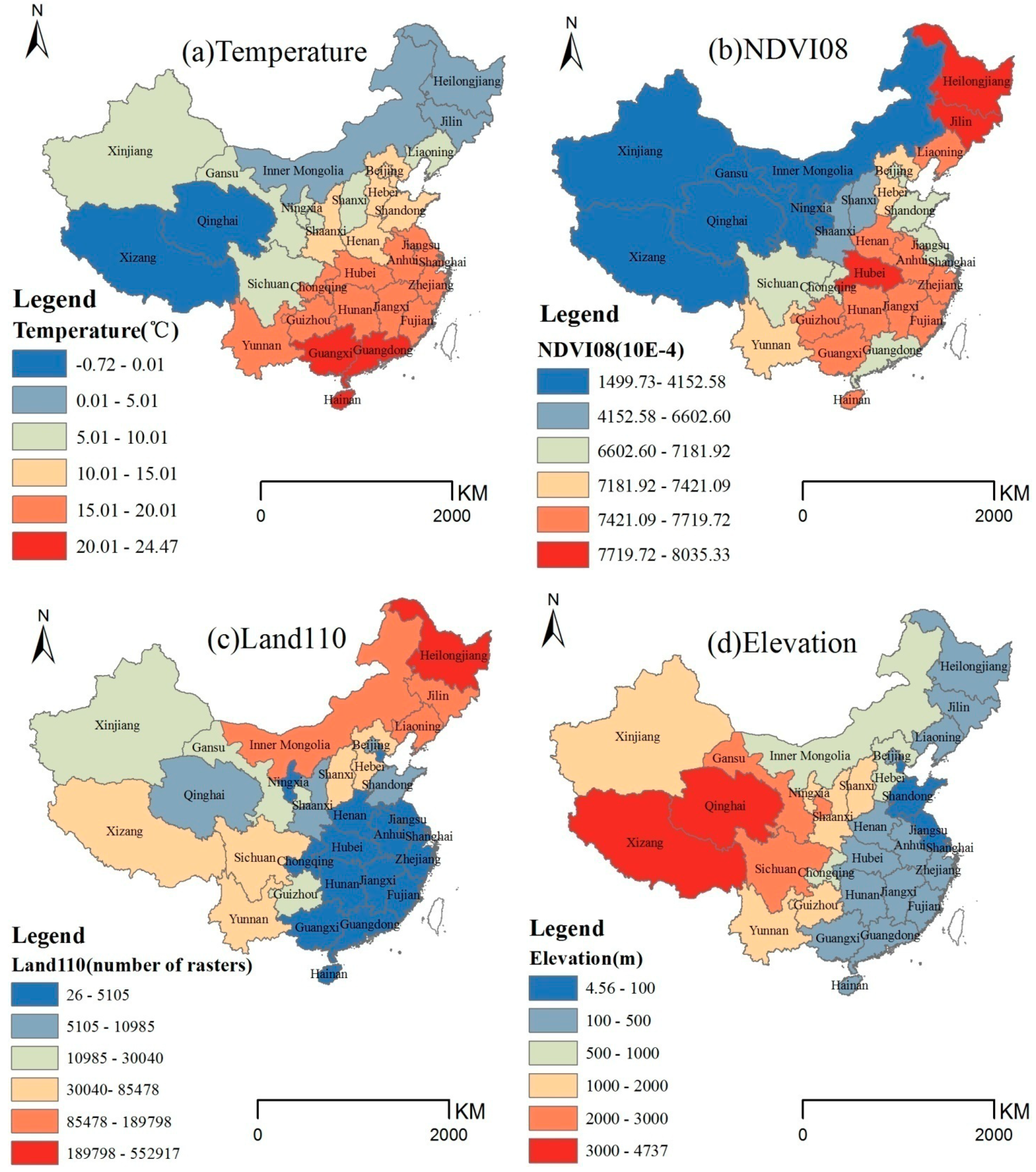
2.1. Data Collection

| Variables | Type and Year | Data Source |
|---|---|---|
| Temperature | Yearly mean temperature | China Meteorological Data Sharing Service System |
| Precipitation | Yearly mean temperature | China Meteorological Data Sharing Service System |
| Humidity | Yearly mean temperature | China Meteorological Data Sharing Service System |
| NDVI | Yearly mean temperature | ftp://ladsweb.nascom.nasa.gov/ |
| NDVI01 | Monthly mean NDVI of January | ftp://ladsweb.nascom.nasa.gov/ |
| NDVI08 | Monthly mean NDVI of January | ftp://ladsweb.nascom.nasa.gov/ |
| Cultivatedland area | Acreage sown to grain | China Statistical Yearbook |
| Grain yield | Grain production | China Statistical Yearbook |
| Land50 | Closed (>40%) broad-leaved deciduous forest (>5 m) | http://due.esrin.esa.int/globcover/ |
| Land100 | Closed to open (>15%) mixed broad-leaved and needle-leaved forest (>5 m) | http://due.esrin.esa.int/globcover/ |
| Land110 | Mosaic forest or shrub-land (50–70%)/grassland (20–50%) | http://due.esrin.esa.int/globcover/ |
| Land120 | Mosaic grassland (50–70%)/forest or shrub-land (20–50%) | http://due.esrin.esa.int/globcover/ |
| Elevation | DEM data | Data Center for Recourses and Environmental Sciences Chinese Academy of Sciences |
2.2. Methods
2.2.1. Spatial Auto-Correlation
2.2.2. Geographically Weighted Regression (GWR) Model
2.3. Data Analyses Using Computer Software
3. Results and Discussion
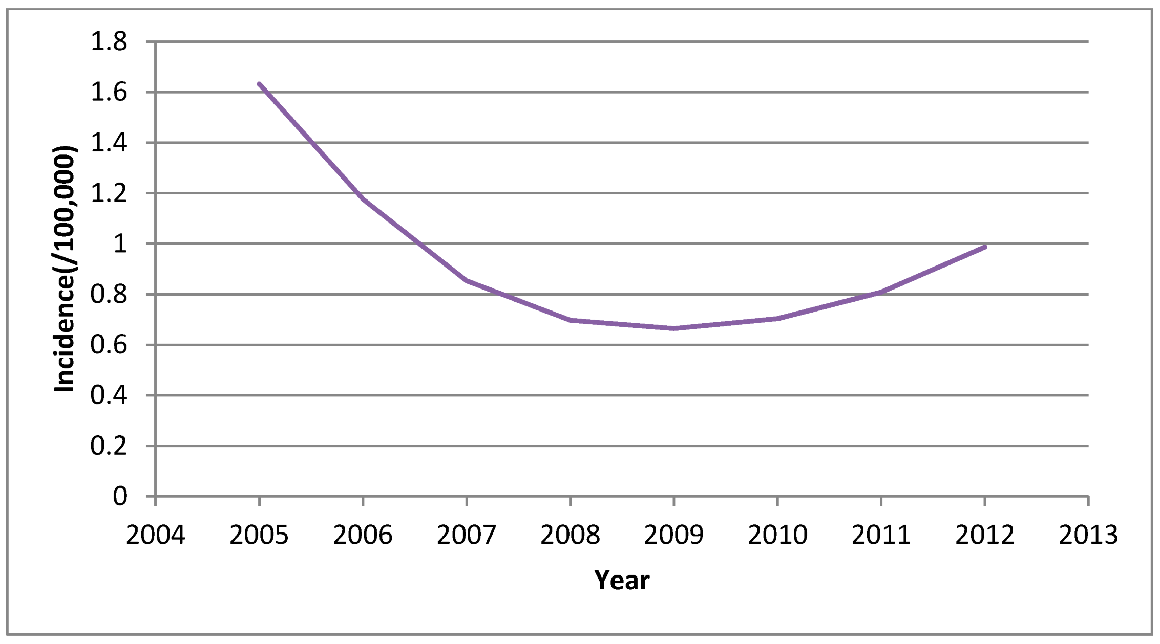
3.1. Descriptive Statistics

3.2. Correlation Analysis

| Potential Related Factors | 2005 | 2006 | 2007 | 2008 | 2009 | 2010 | 2011 | 2012 |
|---|---|---|---|---|---|---|---|---|
| Temperature | −0.390 * | −0.396 * | −0.298 | −0.257 | −0.314 | −0.229 | −0.19 | −0.169 |
| Precipitation | −0.226 | −0.189 | −0.206 | −0.208 | −0.137 | −0.084 | −0.077 | −0.092 |
| Humidity | −0.077 | −0.061 | −0.006 | −0.018 | 0.063 | 0.106 | 0.121 | 0.064 |
| NDVI | −0.075 | −0.047 | 0.003 | 0.026 | 0.004 | 0.023 | 0.048 | 0.056 |
| NDVI01 | −0.389 * | −0.313 | −0.185 | −0.207 | −0.205 | −0.175 | −0.092 | −0.056 |
| NDVI08 | 0.279 | 0.301 | 0.297 | 0.269 | 0.294 | 0.245 | 0.258 | 0.182 |
| Cultivated land area | 0.237 | 0.307 | 0.342 | 0.288 | 0.325 | 0.228 | 0.18 | 0.157 |
| Grain yield | 0.355 * | 0.399 * | 0.380 * | 0.356 * | 0.335 | 0.262 | 0.271 | 0.235 |
| Land50 | 0.612 ** | 0.738 ** | 0.811 ** | 0.727 ** | 0.695 ** | 0.486 ** | 0.460 ** | 0.381 * |
| Land100 | 0.645 ** | 0.758 ** | 0.776 ** | 0.173 | 0.18 | 0.139 | 0.166 | 0.131 |
| Land110 | 0.756 ** | 0.847 ** | 0.861 ** | 0.720 ** | 0.702 ** | 0.481 ** | 0.444 * | 0.365 * |
| Land120 | 0.496 ** | 0.584 ** | 0.613 ** | 0.452 * | 0.448 * | 0.338 | 0.308 | 0.266 |
| Elevation | −0.243 | −0.234 | −0.229 | −0.212 | −0.216 | −0.161 | −0.164 | −0.141 |
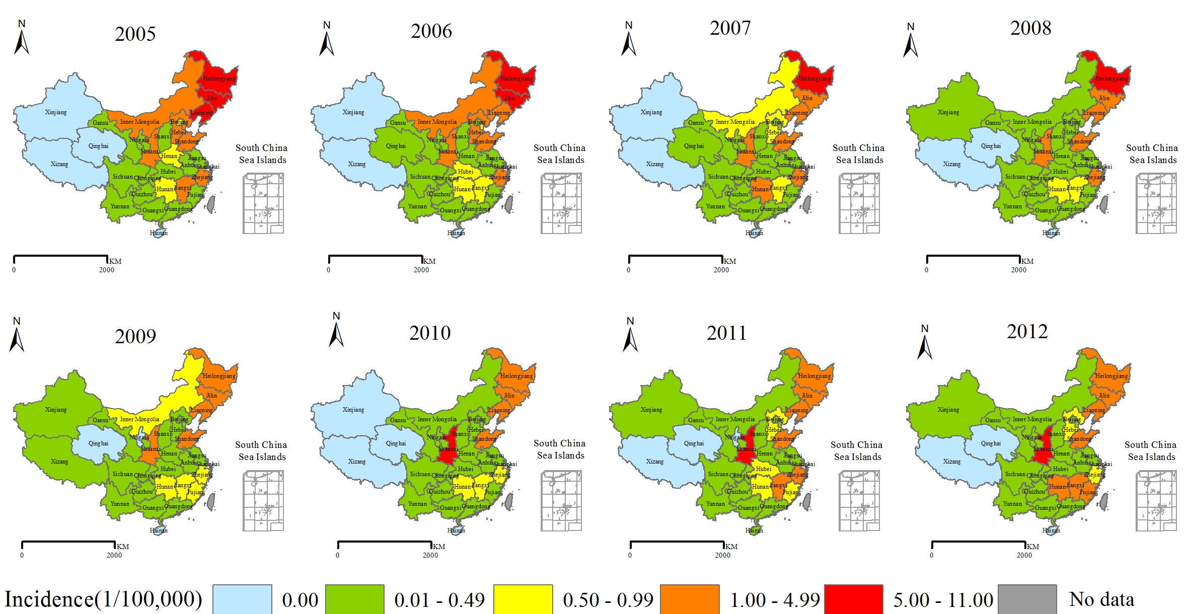
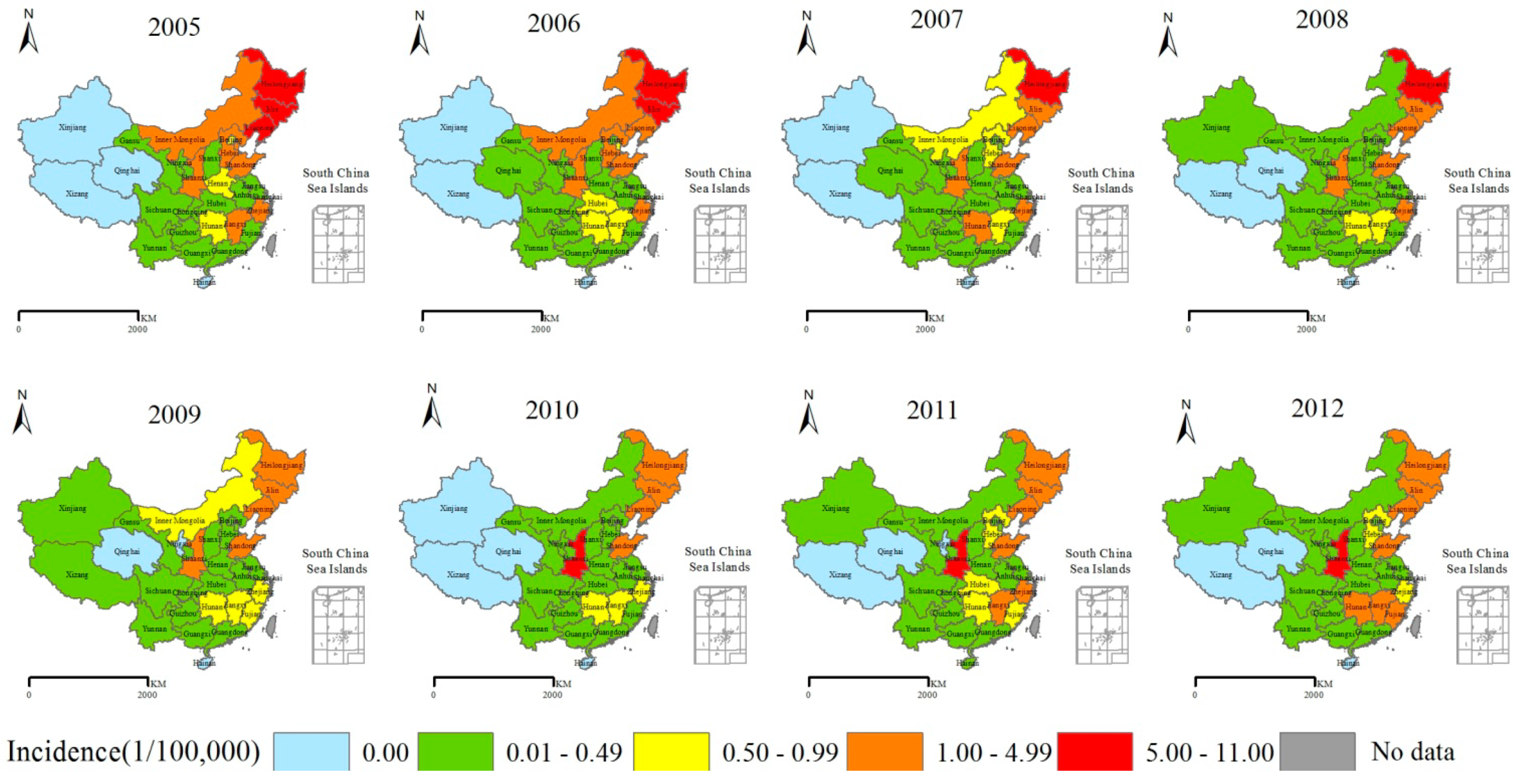
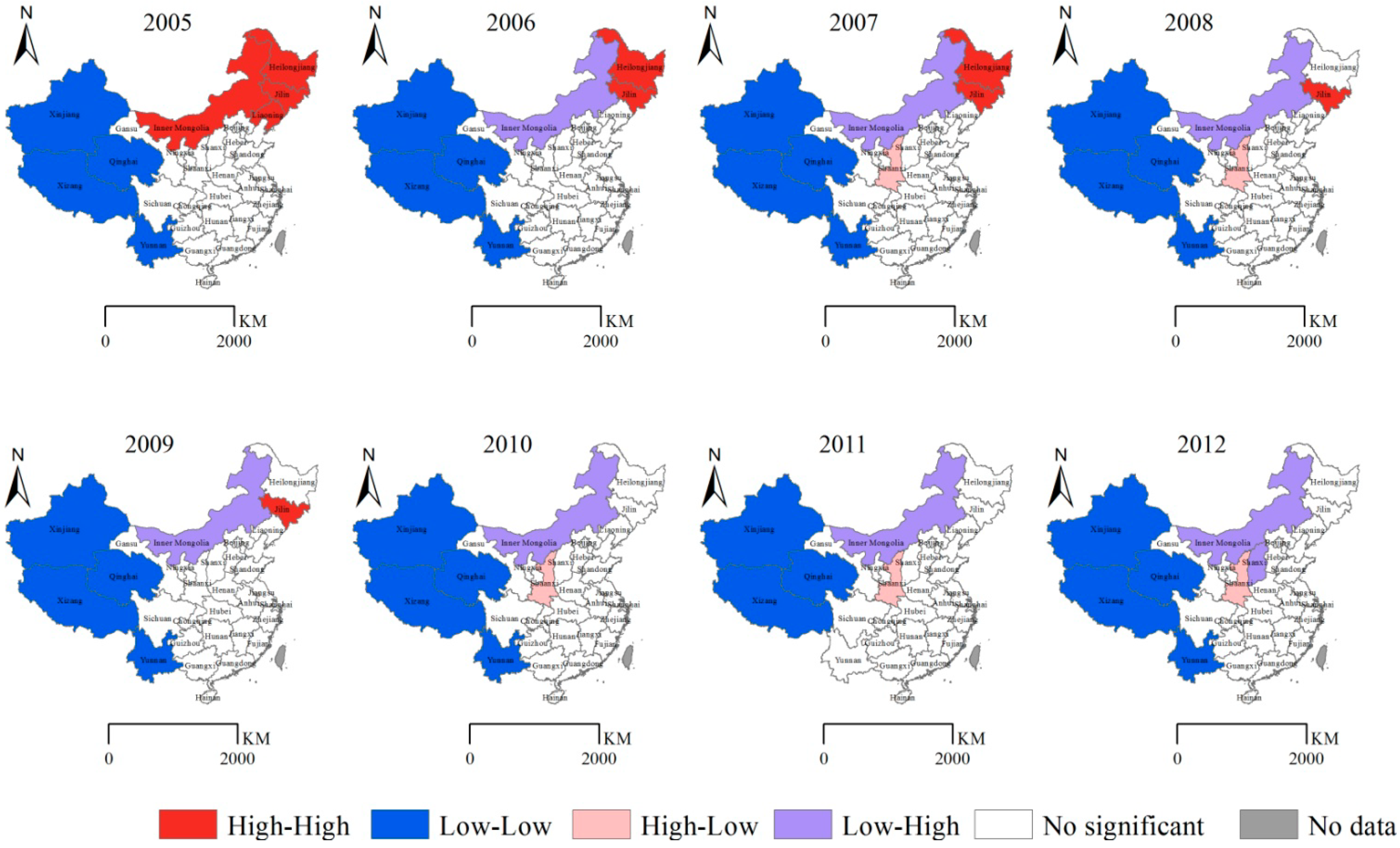
3.3. Spatiotemporal Heterogeneity
| Year | Moran’s I | p |
|---|---|---|
| 2005 | 0.50 | <0.01 |
| 2006 | 0.45 | <0.01 |
| 2007 | 0.28 | <0.01 |
| 2008 | 0.21 | 0.03 |
| 2009 | 0.26 | 0.02 |
| 2010 | 0.05 | 0.18 |
| 2011 | 0.00 | 0.29 |
| 2012 | −0.04 | 0.46 |

3.4. Correlation between HFRS Spatiotemporal Heterogeneity and Related Factors
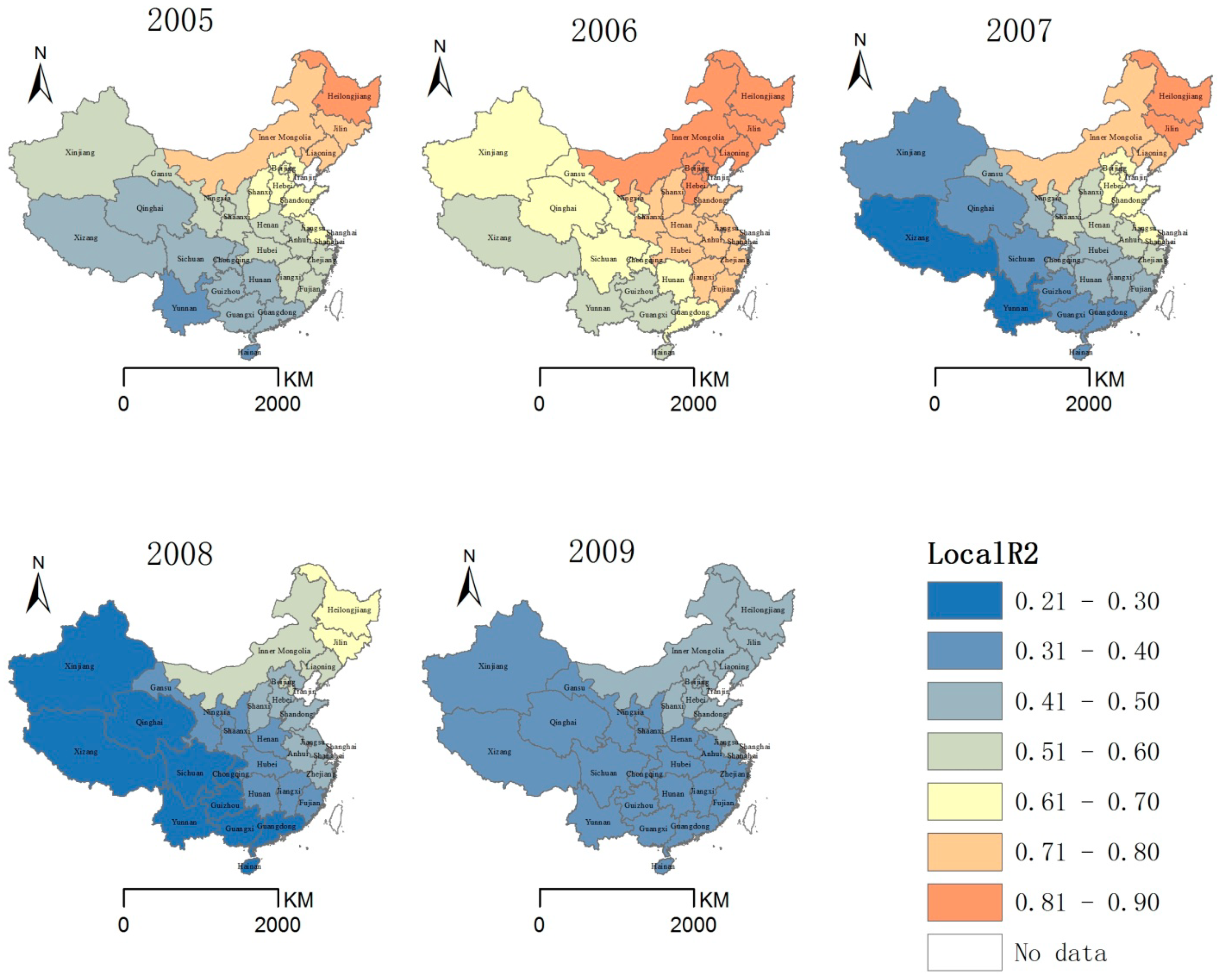
3.4.1. 2005–2009: GWR Modeling and Spatiotemporal Heterogeneity Cause Analysis
| Year | Model | AICc | R2 | R2 adjusted | p |
|---|---|---|---|---|---|
| 2005 | OLS | −583.57 | 0.70 | 0.66 | 0.000 |
| 2005 | GWR | −591.09 | 0.81 | 0.76 | <0.001 |
| 2006 | OLS | −617.29 | 0.84 | 0.81 | 0 |
| 2006 | GWR | −619.38 | 0.88 | 0.84 | <0.001 |
| 2007 | OLS | −620.36 | 0.69 | 0.66 | 0.000 |
| 2007 | GWR | −628.60 | 0.82 | 0.76 | <0.001 |
| 2008 | OLS | −621.64 | 0.48 | 0.42 | 0.001 |
| 2008 | GWR | −616.35 | 0.60 | 0.44 | <0.001 |
| 2009 | OLS | −622.18 | 0.41 | 0.34 | 0.004 |
| 2009 | GWR | −627.27 | 0.63 | 0.55 | <0.001 |

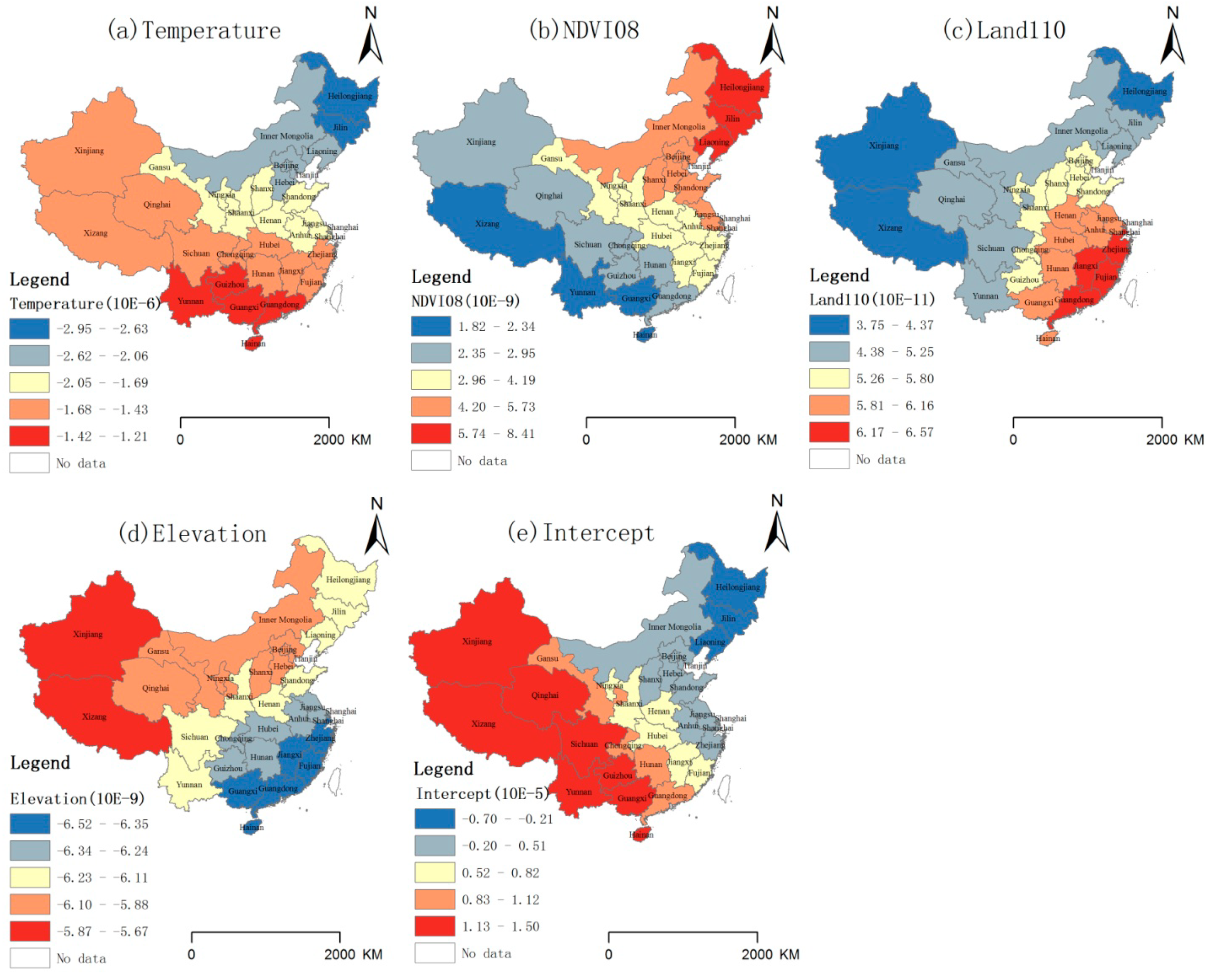
| Year | Temperature 10E−6 | Precipitation 10E−7 | Humidity 10E−7 | NDVI01 10E−9 | NDVI08 10E−9 | Elevation 10E−9 | Land110 10E−11 | Land120 10E−10 |
|---|---|---|---|---|---|---|---|---|
| 2005 | −6.93–−2.29 | 3.20−12.31 | −19.92–−8.69 | |||||
| 2006 | −2.95–−1.21 | 1.82−8.41 | −6.52–−5.67 | 3.75−6.57 | ||||
| 2007 | −7.03–−1.97 | 3.28−14.08 | −26.11–−7.23 | |||||
| 2008 | −1.25–−0.64 | 2.95−5.25 | 0.37−1.95 | |||||
| 2009 | −2.00–−1.55 | 8.41−10.39 | 1.14−1.50 |


3.4.2. 2010–2012: Spatiotemporal Heterogeneity Cause Analysis
4. Conclusions
Acknowledgements
Author Contributions
Conflicts of Interest
References
- Zuo, S.Q.; Fang, L.Q.; Zhan, L.; Zhang, P.H.; Jiang, J.F.; Wang, L.P.; Ma, J.Q.; Wang, B.C.; Wang, R.M.; Wu, X.M.; et al. Geo-spatial hotspots of hemorrhagic fever with renal syndrome and genetic characterization of seoul variants in Beijing, China. PloS Negl. Trop. Dis. 2011, 5. [Google Scholar] [CrossRef]
- Wu, J.; Wang, D.D.; Li, X.L.; de Vlas, S.J.; Yu, Y.Q.; Zhu, J.; Zhang, Y.; Wang, B.; Yan, L.; Fang, L.Q.; et al. Increasing incidence of hemorrhagic fever with renal syndrome could be associated with livestock husbandry in Changchun, Northeastern China. BMC Infect. Dis. 2014, 14. [Google Scholar] [CrossRef] [Green Version]
- Tan, X.; Xiao, D.; Yan, Y. Analysis of epidemic situation of hemorrhagic fever with renal syndrome in huxian, Xi’an, China from 1971 to 2010. Chin. J. Vector Biol. Control 2012, 23, 577–580. [Google Scholar]
- Xiao, H.; Tian, H.Y.; Gao, L.D.; Liu, H.N.; Duan, L.S.; Basta, N.; Cazelles, B.; Li, X.J.; Lin, X.L.; Wu, H.W.; et al. Animal reservoir, natural and socioeconomic variations and the transmission of hemorrhagic fever with renal syndrome in Chenzhou, China, 2006–2010. PloS Negl. Trop. Dis. 2014, 8. [Google Scholar] [CrossRef]
- Lin, H.L.; Zhang, Z.T.; Lu, L.; Li, X.J.; Liu, Q.Y. Meteorological factors are associated with hemorrhagic fever with renal syndrome in Jiaonan county, China, 2006–2011. Int. J. Biometeorol. 2014, 58, 1031–1037. [Google Scholar] [CrossRef] [PubMed]
- Yan, L.; Fang, L.Q.; Huang, H.G.; Zhang, L.Q.; Feng, D.; Zhao, W.J.; Zhang, W.Y.; Li, X.W.; Cao, W.C. Landscape elements and hantaan virus-related hemorrhagic fever with renal syndrome, people’s republic of China. Emerg. Infect. Dis. 2007, 13, 1301–1306. [Google Scholar] [CrossRef] [PubMed]
- Klempa, B. Hantaviruses and climate change. Clin.Microbiol. Infect. 2009, 15, 518–523. [Google Scholar] [CrossRef] [PubMed]
- Haredasht, S.A.; Taylor, C.J.; Maes, P.; Verstraeten, W.W.; Clement, J.; Barrios, M.; Lagrou, K.; Van Ranst, M.; Coppin, P.; Berckmans, D.; et al. Model-based prediction of nephropathia epidemica outbreaks based on climatological and vegetation data and bank vole population dynamics. Zoonoses Public Health 2013, 60, 461–477. [Google Scholar] [CrossRef]
- Liu, H.N.; Gao, L.D.; Chowell, G.; Hu, S.X.; Lin, X.L.; Li, X.J.; Ma, G.H.; Huang, R.; Yang, H.S.; Tian, H.Y.; et al. Time-specific ecologic niche models forecast the risk of hemorrhagic fever with renal syndrome in Dongting Lake district, China, 2005–2010. PloS One 2014, 9. [Google Scholar] [CrossRef]
- Yan, L.; Huang, H.-G.; Zhang, W.-Y. The relationship between hemorrhagic fever with renal syndrome cases and time series of NDVI in Dayangshu District. J. Remote Sens. 2009, 13, 873–886. [Google Scholar]
- Li, Q.; Zhao, W.N.; Wei, Y.M.; Han, X.; Han, Z.Y.; Zhang, Y.B.; Qi, S.X.; Xu, Y.G. Analysis of incidence and related factors of hemorrhagic fever with renal syndrome in Hebei province, China. PloS One 2014, 9. [Google Scholar] [CrossRef] [PubMed]
- Goodin, D.G.; Koch, D.E.; Owen, R.D.; Chu, Y.K.; Hutchinson, J.M.S.; Jonsson, C.B. Land cover associated with hantavirus presence in paraguay. Glob. Ecol. Biogeogr. 2006, 15, 519–527. [Google Scholar] [CrossRef]
- Liu, X.; Jiang, B.; Gu, W.; Liu, Q. Temporal trend and climate factors of hemorrhagic fever with renal syndrome epidemic in Shenyang city, China. BMC Infect. Dis. 2011, 11. [Google Scholar] [CrossRef]
- Xiaodong, L. A Study on the Spatial and Temporal Distribution of HFRS in China and the Impact of Climate Factors on HFRS in Liaoning Province. Ph.D. Thesis, Shandong University, Jinan, China, 2012. [Google Scholar]
- Viel, J.F.; Lefebvre, A.; Marianneau, P.; Joly, D.; Giraudoux, P.; Upegui, E.; Tordo, N.; Hoen, B. Environmental risk factors for haemorrhagic fever with renal syndrome in a French new epidemic area. Epidemiol. Infect. 2011, 139, 867–874. [Google Scholar] [CrossRef] [PubMed]
- Fang, L.Q.; Li, C.Y.; Yang, H.; Chen, H.X.; Li, X.W.; Cao, W.C. Using geographic information system to study on the association between epidemic areas and main animalhosts of hemorrhagic fever with renal syndrome in China. Chin. J. Epidemiol. 2004, 25, 929–933. [Google Scholar]
- Fang, L.Q.; Cao, W.C.; Chen, H.X.; Wang, B.G.; Wu, X.M.; Yang, H.; Zhang, X.T. [Study on the application of geographic information system in spatial distribution of hemorrhage fever with renal syndrome in china]. Chin. J. Epidemiol. 2003, 24, 265–268. [Google Scholar]
- Fang, L.Q.; Cao, W.C.; Dun, Z.; Wu, X.M.; Sun, P.Y.; Kulldorff, M.; Wang, B.C.; Yang, H.; Li, X.W. [Spatial analysis on the distribution of hemorrhagic fever with renal syndrome by geographic information system in Haidian District, Beijing]. Chin. J. Epidemiol. 2003, 24, 1020–1023. [Google Scholar]
- Fang, L.Q.; Zhao, W.J.; de Vlas, S.J.; Zhang, W.Y.; Liang, S.; Looman, C.W.N.; Yan, L.; Wang, L.P.; Ma, J.Q.; Feng, D.; et al. Spatiotemporal dynamics of hemorrhagic fever with renal syndrome, beijing, people's republic of china. Emerging infectious diseases 2009, 15, 2043–2045. [Google Scholar] [CrossRef]
- Fang, L.Q.; Wang, X.J.; Liang, S.; Li, Y.L.; Song, S.X.; Zhang, W.Y.; Qian, Q.A.; Li, Y.P.; Wei, L.; Wang, Z.Q.; et al. Spatiotemporal trends and climatic factors of hemorrhagic fever with renal syndrome epidemic in Shandong province, China. PloS Negl. Trop. Dis. 2010, 4. [Google Scholar] [CrossRef]
- Jonsson, C.B.; Figueiredo, L.T.; Vapalahti, O. A global perspective on hantavirus ecology, epidemiology, and disease. Clin. Microbiol. Rev. 2010, 23, 412–441. [Google Scholar] [CrossRef] [PubMed]
- Zhang, W.Y.; Guo, W.D.; Fang, L.Q.; Li, C.P.; Bi, P.; Glass, G.E.; Jiang, J.F.; Sun, S.H.; Qian, Q.; Liu, W.; et al. Climate variability and hemorrhagic fever with renal syndrome transmission in Northeastern China. Environ. Health Perspect. 2010, 118, 915–920. [Google Scholar] [CrossRef]
- Bi, P.; Wu, X.K.; Zhang, F.Z.; Parton, K.A.; Tong, S.L. Seasonal rainfall variability, the incidence of hemorrhagic fever with renal syndrome, and prediction of the disease in low-lying areas of china. Am.J. Epidemiol. 1998, 148, 276–281. [Google Scholar] [CrossRef] [PubMed]
- Xiao, H.; Lin, X.L.; Gao, L.D.; Huang, C.R.; Tian, H.Y.; Li, N.; Qin, J.X.; Zhu, P.J.; Chen, B.Y.; Zhang, X.X.; et al. Ecology and geography of hemorrhagic fever with renal syndrome in Changsha, China. BMC Infect. Dis. 2013, 13, 11. [Google Scholar] [CrossRef]
- Zhang, S.; Wang, S.W.; Yin, W.W.; Liang, M.F.; Li, J.D.; Zhang, Q.F.; Feng, Z.J.; Li, D.X. Epidemic characteristics of hemorrhagic fever with renal syndrome in China, 2006–2012. BMC Infect. Dis. 2014, 14. [Google Scholar] [CrossRef] [PubMed]
- Anselin, L.; Syabri, I.; Kho, Y. Geoda: An introduction to spatial data analysis. Geogr. Anal. 2006, 38, 5–22. [Google Scholar] [CrossRef]
- Unwin, D.; Unwin, A. Local indicators of spatial association—Foreword. J. Roy. Stat. Soc. D-Sta. 1998, 47, 413. [Google Scholar] [CrossRef]
- Moran, P.A.P. The interpretation of statistical maps. J. Roy. Stat. Soc. B 1948, 10, 243–251. [Google Scholar]
- David, F.N. Spatial autocorrelation—Cliff,ad and ord,jk. Biometrics 1974, 30, 729. [Google Scholar] [CrossRef]
- Lebanon, A. Spatial autocorrelation—Cliff,ad and ord,jk. J. Am. Stat. Assoc. 1974, 69, 834–835. [Google Scholar] [CrossRef]
- Zhang, C.; Luo, L.; Xu, W.; Ledwith, V. Use of local moran’s I and gis to identify pollution hotspots of pb in urban soils of Galway, Ireland. Sci. Total Environ. 2008, 398, 212–221. [Google Scholar] [CrossRef] [PubMed]
- Fotheringham, A.S.; Brunsdon, C.; Charlton, M. Geographically Weighted Regression—The Analysis of Spatially Varying Relationships; John Wiley & Sons Ltd.: WestSussex, UK, 2002. [Google Scholar]
- Yang, L.X.; Yang, G.S.; Yao, S.M.; Yuan, S.F. A study on the spatial heterogeneity of grain yield per hectare and driving factors based on Esda-Gwr. Econ. Geogr. 2012, 32, 120–127. [Google Scholar]
- Lin, G.; Fu, J.Y.; Jiang, D.; Hu, W.S.; Dong, D.L.; Huang, Y.H.; Zhao, M.D. Spatio-temporal variation of pm2.5 concentrations and their relationship with geographic and socioeconomic factors in china. Int. J. Env. Res. Public Health 2014, 11, 173–186. [Google Scholar] [CrossRef]
- Yao, W.Q.; Guo, J.Q.; Sun, Y.W.; Liu, M.; Han, Y.H.; Zhao, Z. Evaluation on effect of comprehensive intervention measure on hemorrhagic fever with renal syndrome. Chin. J. Epidemiol. 2008, 24, 1361–1362. [Google Scholar]
- Xiao, H.; Lin, X.L.; Gao, L.D.; Dai, X.Y.; He, X.G.; Chen, B.Y.; Zhang, X.X.; Zhao, J.; Tian, H.Y. Environmental factors contributing to the spread of hemorrhagic fever with renal syndrome and potential risk areas prediction in midstream and downstream of the Xiangjiang River. Sci. Geogr. Sin. 2013, 33, 123–128. [Google Scholar]
- Xiao, H.; Liu, H.N.; Gao, L.D.; Huang, C.R.; Li, Z.; Lin, X.L.; Chen, B.Y.; Tian, H.Y. Investigating the effects of food available and climatic variables on the animal host density of hemorrhagic fever with renal syndrome in Changsha, China. PloS One 2013, 8. [Google Scholar] [CrossRef] [PubMed]
- Zhang, Y.H.; Ge, L.; Liu, L.; Huo, X.X.; Xiong, H.R.; Liu, Y.Y.; Liu, D.Y.; Luo, F.; Li, J.L.; Ling, J.X.; et al. The epidemic characteristics and changing trend of hemorrhagic fever with renal syndrome in Hubei province, China. PloS One 2014, 9. [Google Scholar] [CrossRef]
- Xiao, H.; Tian, H.Y.; Cazelles, B.; Li, X.J.; Tong, S.L.; Gao, L.D.; Qin, J.X.; Lin, X.L.; Liu, H.N.; Zhang, X.X. Atmospheric moisture variability and transmission of hemorrhagic fever withrenal syndrome in Changsha city, mainland China, 1991–2010. PloS Negl. Trop. Dis. 2013, 7. [Google Scholar] [CrossRef] [PubMed]
- Zuo, S.Q.; Fang, L.Q.; Zhan, L.; Zhang, P.H.; Jiang, J.F.; Wang, L.P.; Ma, J.Q.; Wang, B.C.; Wang, R.M.; Wu, X.M.; et al. Geo-spatial hotspots of hemorrhagic fever with renal syndrome and genetic characterization of seoul variants in Beijing, China. PloS Negl. Trop. Dis. 2011, 5. [Google Scholar] [CrossRef] [PubMed]
- Yu, H.Y.; Liu, S.H.; Zhao, N.; Li, D.; Yu, Y.T. Characteristics of air temperature and precipitation in different regions of China from 1951 to 2009. J. Meteorol. Environ. 2011, 27, 1–11. [Google Scholar]
- Tang, G.; Ding, Y.; Wang, S.; Ren, G.; Liu, H.; Zhang, L. Comparative analysis of the time series of surface air temperature over china for the last 100 years. Adv.Clim. Change Res. 2009, 5. [Google Scholar] [CrossRef]
- Zhang, Y.Z.; Zhang, H.L.; Dong, X.Q.; Yuan, J.F.; Zhang, H.J.; Yang, X.L.; Zhou, P.; Ge, X.Y.; Li, Y.; Wang, L.F.; et al. Hantavirus outbreak associated with laboratory rats in Yunnan, China. Infect. Genet. Evol. 2010, 10, 638–644. [Google Scholar] [CrossRef] [PubMed]
- Li, J.S.; Chen, Z.J.; Hou, T.J.; Xing, Y.; Cai, Z.H.; Yang, Y. Study on the risk factors of hemorrhagic fever with renal syndrome in Xi’an city. Chin. J. Dis. Control Prev. 2013, 17, 564–566. [Google Scholar]
- Ma, C.F.; Wang, Z.G.; Li, S.; Xing, Y.; Wu, R.; Wei, J.; Nawaz, M.; Tian, H.Y.; Xu, B.; Wang, J.J.; et al. Analysis of an outbreak of hemorrhagic fever with renal syndrome in college students in Xi’an, China. Viruses 2014, 6, 507–515. [Google Scholar] [CrossRef] [PubMed]
- Barrios, J.M.; Verstraeten, W.W.; Maes, P.; Clement, J.; Aerts, J.M.; Haredasht, S.A.; Wambacq, J.; Lagrou, K.; Ducoffre, G.; Van Ranst, M.; et al. Satellite derived forest phenology and its relation with nephropathia epidemica in Belgium. Int. J. Environ. Res. Public Health 2010, 7, 2486–2500. [Google Scholar] [CrossRef] [PubMed]
© 2014 by the authors; licensee MDPI, Basel, Switzerland. This article is an open access article distributed under the terms and conditions of the Creative Commons Attribution license (http://creativecommons.org/licenses/by/4.0/).
Share and Cite
Li, S.; Ren, H.; Hu, W.; Lu, L.; Xu, X.; Zhuang, D.; Liu, Q. Spatiotemporal Heterogeneity Analysis of Hemorrhagic Fever with Renal Syndrome in China Using Geographically Weighted Regression Models. Int. J. Environ. Res. Public Health 2014, 11, 12129-12147. https://doi.org/10.3390/ijerph111212129
Li S, Ren H, Hu W, Lu L, Xu X, Zhuang D, Liu Q. Spatiotemporal Heterogeneity Analysis of Hemorrhagic Fever with Renal Syndrome in China Using Geographically Weighted Regression Models. International Journal of Environmental Research and Public Health. 2014; 11(12):12129-12147. https://doi.org/10.3390/ijerph111212129
Chicago/Turabian StyleLi, Shujuan, Hongyan Ren, Wensheng Hu, Liang Lu, Xinliang Xu, Dafang Zhuang, and Qiyong Liu. 2014. "Spatiotemporal Heterogeneity Analysis of Hemorrhagic Fever with Renal Syndrome in China Using Geographically Weighted Regression Models" International Journal of Environmental Research and Public Health 11, no. 12: 12129-12147. https://doi.org/10.3390/ijerph111212129