Cross-Country Assessment of H-SAF Snow Products by Sentinel-2 Imagery Validated against In-Situ Observations and Webcam Photography

Abstract

Information on snow properties is of critical relevance for a wide range of scientific studies and operational applications, mainly for hydrological purposes. However, the ground-based monitoring of snow dynamics is a challenging task, especially over complex topography and under harsh environmental conditions. Remote sensing is a powerful resource providing snow observations at a large scale. This study addresses the potential of using Sentinel-2 high-resolution imagery to assess moderate-resolution snow products, namely H10—Snow detection (SN-OBS-1) and H12—Effective snow cover (SN-OBS-3) supplied by the Satellite Application Facility on Support to Operational Hydrology and Water Management (H-SAF) project of the European Organisation for the Exploitation of Meteorological Satellites (EUMETSAT). With the aim of investigating the reliability of reference data, the consistency of Sentinel-2 observations is evaluated against both in-situ snow measurements and webcam digital imagery. The study area encompasses three different regions, located in Finland, the Italian Alps and Turkey, to comprehensively analyze the selected satellite products over both mountainous and flat areas having different snow seasonality. The results over the winter seasons 2016/17 and 2017/18 show a satisfying agreement between Sentinel-2 data and ground-based observations, both in terms of snow extent and fractional snow cover. H-SAF products prove to be consistent with the high-resolution imagery, especially over flat areas. Indeed, while vegetation only slightly affects the detection of snow cover, the complex topography more strongly impacts product performances.

1. Introduction

The knowledge of the extent and location of snow cover is of key importance to enhance the understanding of the present and future climate, hydrological cycle, and ecological dynamics, at both local and global scales [1,2]. Indeed, snow-dominated regions serve as an active reservoir for water supply during the melting period [3,4], and the seasonal presence of snow cover significantly modulates a surface energy balance because of its high albedo and thermal properties [5]. Therefore, information on the spatial and temporal distribution of snow cover is critical for several research purposes and operational applications [6]. However, the monitoring of a snow-covered area is generally hindered by the complex interactions among site-dependent factors, especially in mountainous and forested regions. Meteorological forcings (i.e., precipitation regime, average air temperature, solar radiation) [7,8,9] and local topography (i.e., elevation, slope orientation and mean aspect) [10,11,12] are the most explanatory variables affecting spatial and temporal variability and persistence of snow cover. The definition of the topographic control on snow distribution is made challenging by the presence of vegetation, which intercepts snowfall and impacts the intensity of meteorological forcings [13,14,15]. Furthermore, wind-induced erosion and deposition phenomena are the main control factors driving the snow’s spatial redistribution [16,17]. In-situ automatic measurements provide continuous and direct observational data allowing the retrieval of a temporal evolution of snow cover. However, they are site-dependent, generally subjected to distortions (e.g., wind action, vegetation interactions), and they do not succeed in catching the spatial variability of snowpack due to the heterogeneity of both climate and terrain with respect to the network density [18,19]. The collection of in-situ measurements at a large scale necessarily faces a general widespread lack of instrumental records, especially for steep slopes and remote high-elevation areas, where harsh environmental conditions usually entail a high operating cost [20].

Among in-situ gauges, the time-lapse camera is renowned for being a cost-effective device to monitor many environmental variables for scientific purposes [21,22,23,24,25]. Several webcam networks are currently operational worldwide, such as the European phenology camera network (EUROPhen) [26], the PhenoCam Network [27], and MONIMET camera network [24]. Recently, a growing interest aims at using webcam photography to detect snow cover from digital images to monitor its variability in space and time, even though the use of these observations is restricted to limited spatial scales [12,28,29,30,31,32,33,34].

Remote sensing represents a suited and powerful tool to monitor snow properties at larger scales and to overcome the gradual decrease of the representativeness of the gauging network with the increasing altitude. Under specific conditions (e.g., day-time, absence of cloudiness) [35], the snow cover detection is relatively straightforward through satellite-based optical observations, because of the high albedo of snow with respect to most land surfaces and the higher near-infrared reflectance of most clouds compared to snow-covered surfaces [36,37]. As well as cloud cover, the vegetation can obstruct visible and infrared information about snow, especially where forest canopy protruding above the snowpack reduces the surface albedo [38] and partially or completely shades the underlying surface [39,40]. Nevertheless, since satellite-based data are indirect measurements of snow-related quantities, they require a quantitative understanding of their accuracy, mainly depending on the uncertainty in retrieval algorithms [37,41]. Therefore, the comprehensive validation of satellite snow products is of key importance to properly assess and quantify their reliability, to identify possible errors and to provide input for further improvements. Indeed, the availability of information on the quality control of remotely-sensed data is critically needed by the scientific community, as one of the main key criteria for the selection of the most proper dataset to be effectively used, according to the final purpose.

Numerous studies have addressed the validation of satellite snow products at local and global scale by assessing the accuracy of remotely-sensed observations against ground-based data, which is one of the most widely used validation procedures [42,43,44,45,46,47,48,49,50,51,52,53,54]. Lacking any available in-situ reference data, a common approach relies on a cross-sensor comparison among different satellite-derived snow products by assuming one of the analyzed datasets as the reference truth [55,56,57,58]. This approach is even necessary when assessing the accuracy of satellite-derived products of fractional snow cover (FSC) requiring spatially distributed observations of reference [33]. Even though currently there is no agreed-upon methodology to perform a cross-sensor comparison, the most commonly used approach assumes the high-resolution satellite imagery as the reference effective dataset to assess moderate-resolution remotely-sensed observations, since it is supposed to provide the most reliable information on the actual snow cover [59]. Nowadays, the Sentinel-2 (S-2) mission of European Copernicus Earth Observation program provides high-resolution multispectral imagery with an operational short revisiting time (~5 days) and free, global and systematic availability. Because of its meaningful payload, several studies have already experienced the potentialities of S-2 data in different fields of application [60,61,62,63,64,65].

This study aims to investigate the potential use of S-2 data to assess the reliability of moderate-resolution products of snow extent and FSC, that are the snow-related quantities most commonly used as input for hydrologic, meteorological and climate modelling [2]. Indeed, H10—Snow detection (SN-OBS-1) and H12—Effective snow cover (SN-OBS-3) supplied by the EUMETSAT’s H-SAF project are compared against S-2 imagery. The interest in H-SAF snow products is focused on investigating the potential of these datasets and their suitability for hydrological purposes [56]. Over past decades, operational H-SAF snow products have been continuously validated against ground-based snow measurements [53,56]. Even though the high-resolution imagery can be reasonably used to establish reliable ground truth, a finer spatial resolution does not necessarily entail a higher accuracy of the satellite product, since its accuracy strongly depends on the retrieval algorithm used to derive snow-related information. Furthermore, no existing study supplies detailed information on the accuracy of S-2 imagery in detecting snow. For these reasons, the study has therefore the dual objective of validating this high-resolution dataset against in-situ snow measurements and webcam photography in order to properly assess its consistency and to guarantee the reliability of the comparison analysis. Therefore, before addressing the cross-sensor comparison of snow satellite products, a comprehensive validation of S-2 data is performed against ground-based data. With the aim of testing and assessing the satellite snow products under different climatological and topographic conditions, three study areas located in Finland, the Italian Alps, and Turkey are analyzed.

After introducing the context of this study, its motivation and research purposes, the article consists of four main sections. Section 2 is focused on data collection through a comprehensive description of the analyzed remotely-sensed (i.e., S-2, H-SAF H10 and H12) and ground-based (i.e., snow depth measurements and webcam imagery) datasets. The selected case studies in Finland, Italy and Turkey are presented and characterized. In Section 3, the methodology is extensively explained into the details of the retrieval algorithms for the generation of satellite products. The procedures implemented within both the validation of S-2 imagery against in-situ data, and the comparison between S-2-based and moderate-resolution snow products are widely described and their main assumptions are discussed. Results are reported and assessed through several evaluation metrics in Section 4. Lastly, conclusions are outlined in Section 5.

2. Materials

2.1. Satellite Datasets

2.1.1. Sentinel-2 Imagery

S-2 is a polar-orbiting, multispectral high-resolution imaging mission of the European Space Agency (ESA) for land, ocean and atmospheric monitoring. With the aim of fulfilling revisit and coverage requirements and providing robust datasets, the constellation consists of two identical satellites, Sentinel-2A (S-2A) and Sentinel-2B (S-2B), which were launched on 23 June 2015 (operational in early 2016) and 7 March 2017, respectively. Since the twin satellites are in the same sun-synchronous orbit with a phase delay of 180°, they guarantee an effective revisit time of 5 days at the equator and 2/3 days over mid-latitudes, with a 290-km swath width. Multi-Spectral Imager (MSI) instruments provide fine spatial resolution optical images (Figure 1) having 13 bands spanning from the visible and the near infrared to the shortwave infrared, covering wavelengths from 0.4 to 2.2 μm (

Table 1. Spatial resolution and central wavelength of Sentinel-2A and -2B spectral bands.

Band Number	Spatial Resolution [m]	S-2A Central Wavelength [nm]	S-2B Central Wavelength [nm]
1	60	442.7	442.2
2	10	492.4	492.1
3	10	559.8	559.0
4	10	664.6	664.9
5	20	704.1	703.8
6	20	740.5	739.1
7	20	782.8	779.7
8	10	832.8	832.9
8a	20	864.7	864.0
9	60	945.1	943.2
10	60	1373.5	1376.9
11	20	1613.7	1610.4
12	20	2202.4	2185.7

) [66]. Depending on the spectral band, the spatial resolution varies from 10 to 60 m. Four visible and near-infrared (VNIR) bands at 10 m for optical measurement, four NIR bands at 20 m for vegetation red-edge, two shortwave infrared (SWIR) bands at 20 m for snow, ice, and cloud discrimination, three coarse bands at 60 m in the aerosol, water vapor, and cirrus domain designated for atmospheric correction [67,68]. However, it is noteworthy that S-2 does not have a thermal band, which is of key importance for cloud detection, as cloud pixels are much colder than clear-sky pixels [69]. By December 2015, the acquisition of S-2 Level-1C (L1C) top-of-atmosphere (TOA) reflectance data is available and currently also S-2 Level-2A (L2A) bottom-of-atmosphere (BOA) reflectance data product is available to the remote sensing community worldwide.

2.1.2. H-SAF H10 Product

H-SAF H10 (SN-OBS-1) is a daily operational product of snow extent generated from the visible (VIS) and infrared (IR) radiometry of the Spinning Enhanced Visible and Infrared Imager (SEVIRI) instrument on board the geostationary Meteosat Second Generation (MSG) satellites. The high temporal resolution and wide aerial coverage of SEVIRI imagery make it highly suitable for snow-cover mapping, since cloud cover is continuously monitored. Indeed, the daily snow cover product is derived for a multi-temporal analysis of SEVIRI 15-min images, that are processed as new data are available to collect the largest possible number of cloud-free pixels. The sampling is performed at 3-km intervals, which degrade to ~5 km over Europe. The resulting daily map has a spatial coverage delimited between longitude 25° W–45° E and latitude 25°–75° N [56,70] and it consists of four different classes: snow, cloud, water and bare ground (Figure 2).

2.1.3. H-SAF H12 Product

H-SAF H12 (SN-OBS-3) is a daily operational product of FSC based on the multi-channel analysis of the Advanced Very High Resolution Radiometer (AVHRR) on board National Oceanic and Atmospheric Administration (NOAA) and meteorological operational (MetOp) satellites. FSC is generated at pixel resolution by exploiting the brightness intensity, which is the convolution of the snow signal and the fraction of snow within the pixel.

The sampling is carried out at 1 km intervals over the same H-SAF area of H10 product. The thematic map includes cloud and water classes, and percentage classes of fraction snow cover ranging from 0% (i.e., snow-free condition) to 100% (i.e., full snow cover) (Figure 3).

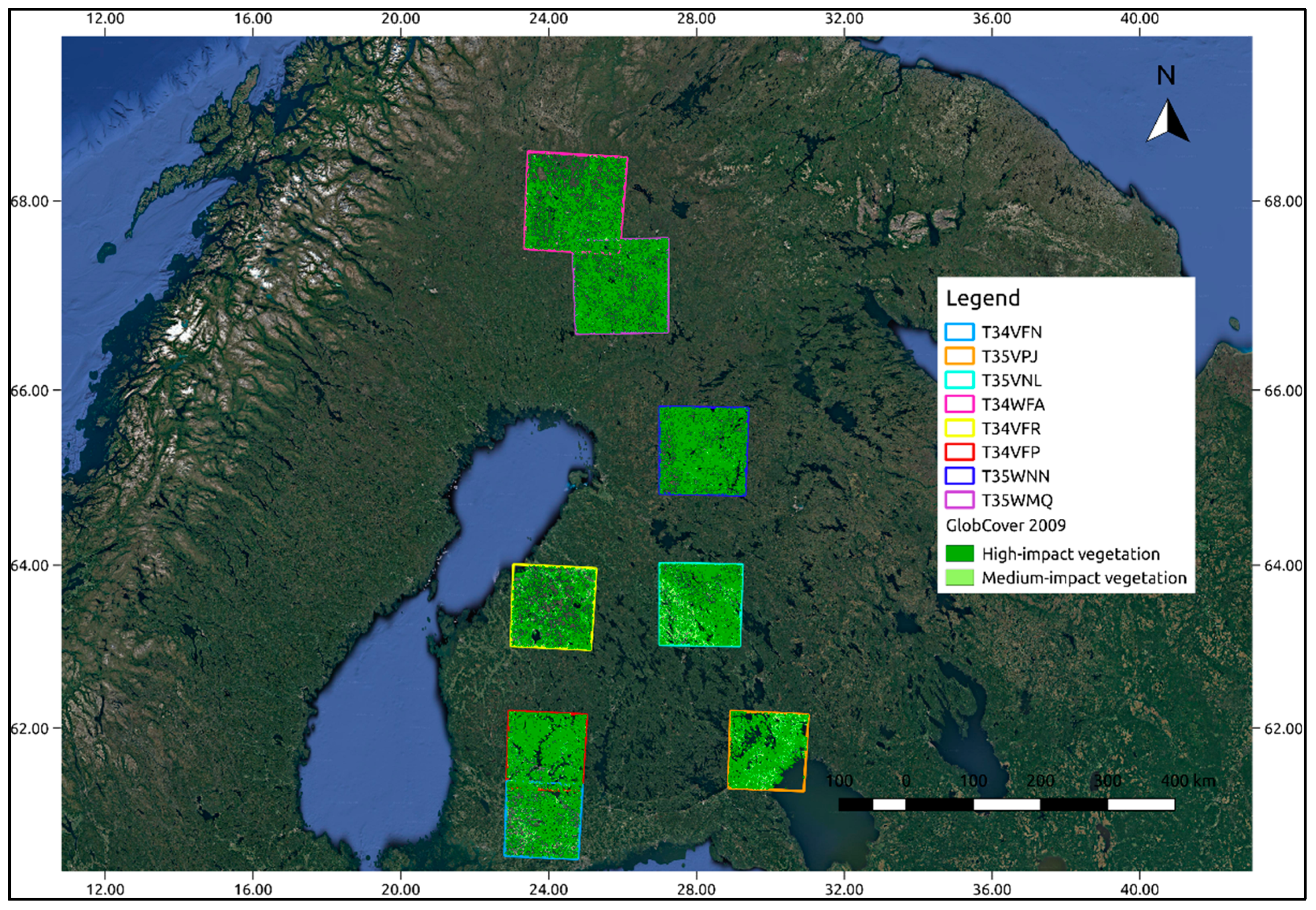
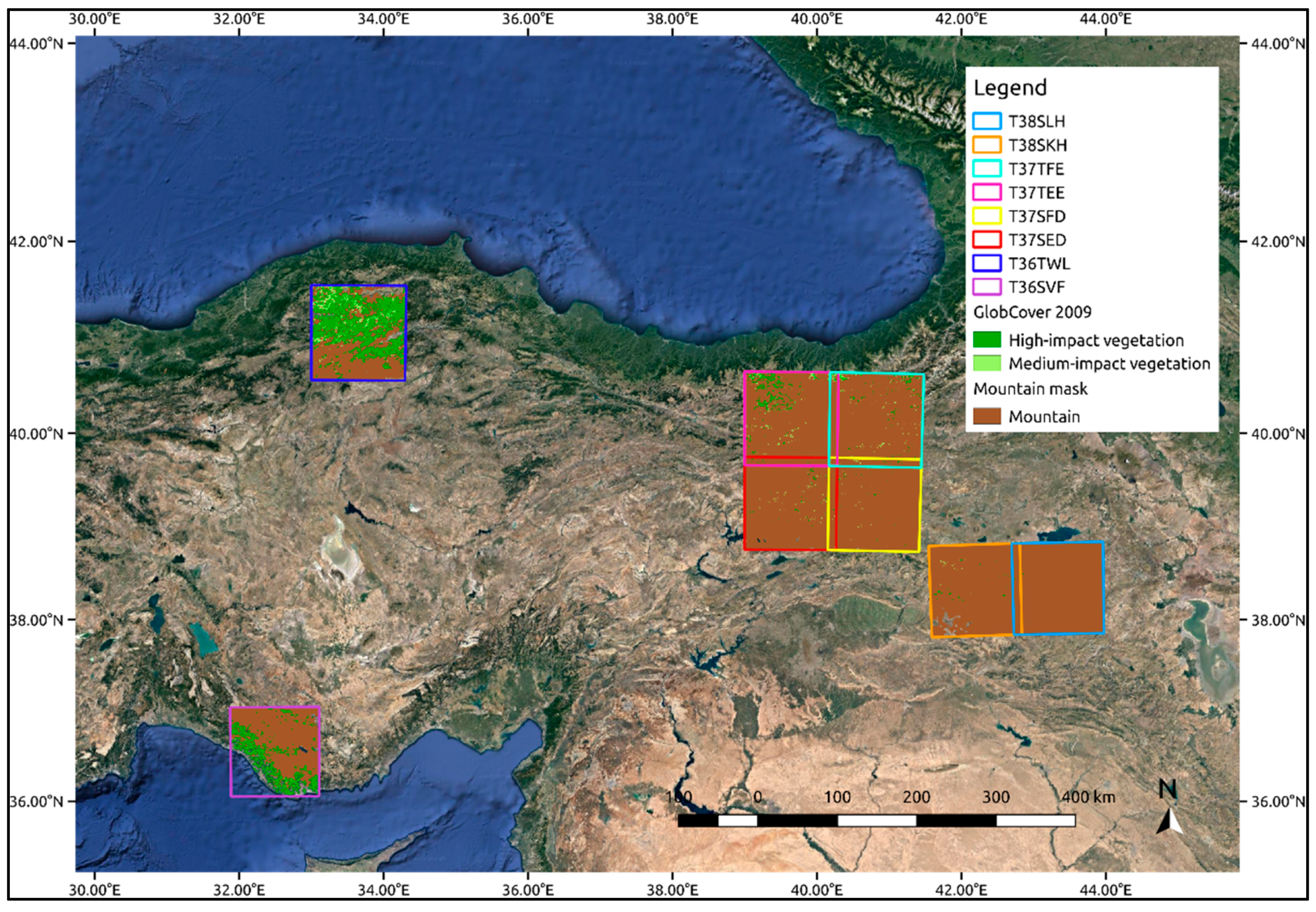
2.2. Test Sites and Data Collection

With the aim of properly investigating the reliability of satellite snow products and their consistency under different topographical conditions (i.e., mountainous and flat areas) and vegetation cover, this study includes three case studies located in Finland, the Italian Alps and Turkey (Figure 4, Figure 5 and Figure 6). In each country, eight S-2 tiles of interest have been selected to properly ensure a sizeable sample of satellite images. The selection of S-2 tiles has targeted those providing significant datasets over the analyzed period by minimizing possible overlapping. Furthermore, when selecting S-2 tiles the location of in-situ monitoring instruments has been considered to allow the validation of S-2 imagery against ground-based data. It is noteworthy to consider that in this study both snow extent and FSC are referred to the snow cover viewable over the satellite field of view, and not at the ground level. Because of the significant impact of vegetation on satellite snow detection, ancillary information on the vegetation cover of each S-2 tile has been derived from ESA GlobCover 2009 land cover map to support the assessment of the comparison results. This GlobCover map is derived from an automated classification of the Medium Resolution Imaging Spectrometer Full Resolution (MERIS FR) time series and it consists of 22 land-cover classes at a 300 m spatial resolution. Among the classes of natural and semi-natural terrestrial vegetation, two main categories have been defined (

Table 2. Selected vegetation classes of ESA GlobCover product.

Vegetation Class	Selection of GlobCover Vegetation Classes
V_1	Closed to open (>15%) broadleaved evergreen and/or semi-deciduous forest (>5 m)
	Closed (>40%) needle-leaved evergreen forest (>5 m)
	Open (15–40%) needle-leaved deciduous or evergreen forest (>5 m)
	Closed to open (>15%) mixed broadleaved and needle-leaved forest (>5 m)
V_2	Closed (>40%) broadleaved deciduous forest (>5 m)
	Open (15–40%) broadleaved deciduous forest (>5 m)

). The first main category embraces the vegetation classes having the highest impact on snow detection (V_1) (i.e., evergreen or semi-deciduous forest), while the second one includes those having a lower impact (V_2) (i.e., deciduous forest).

The selected tiles are reported in

Table 3. Selection of S-2 tiles at each test site and characterization of vegetation cover according to GlobCover 2009 land cover map. Two main vegetation classes having high (V_1) and medium (V_2) impact on snow detection are reported.

Selection of S-2 Tiles
Finland	T34VFN	T34VFP	T34VFR	T34WFA	T35VNL	T35VPJ	T35WMQ	T35WNN
V_1	53%	73%	45%	57%	62%	57%	69%	73%
V_2	10%	6%	8%	2%	17%	14%	2%	2%
Italy	T32TLQ	T32TLR	T32TMR	T32TMS	T32TNS	T32TPS	T32TQS	T33TUM
V_1	10%	13%	6%	17%	20%	34%	33%	30%
V_2	15%	12%	19%	15%	12%	14%	21%	22%
Turkey	T36SVF	T36TWL	T37SED	T37SFD	T37TEE	T37TFE	T38SKH	T38SLH
V_1	17%	41%	1%	0%	5%	2%	0%	0%
V_2	0%	6%	0%	0%	2%	1%	0%	0%

, where the percentage values of the main vegetation categories are reported according to the GlobCover 300 m land cover map.

The analysis period extends throughout two winter seasons, namely 2016/2017 and 2017/2018. With the aim of properly taking account of the local climatology, the duration of the snow season has been independently set from October to May (eight months) in Finland and over the Italian Alps, and from November to April (six months) in Turkey.

Since this study is focused on assessing how satellite products succeed in detecting snow cover, cloud free scenes or scenes with minor cloud cover are primarily selected. Indeed, only S-2 images with cloud cover lower than 20% have been included in the analysis.

The resulting datasets of S-2 imagery for the analyzed case studies are reported in

Table 4. Seasonal effective number of S-2 images at each test site.

Test Site	Seasonal Number of S-2 Images
	Snow Season 2016/17	Snow Season 2017/18
Finland	60	193
Italian Alps	133	198
Turkey	37	101

. It is noteworthy to consider that the effective number of S-2 images in the snow season 2017/2018 is significantly higher than in the previous one (Table 4), since S-2B data has become available in March 2017.

Throughout the analyzed period, only one daily H10 image is missing during the first snow season and 7 images are missing in the second one. Likewise, H12 product is not available for 7 and 16 days in snow seasons 2016/17 and 2017/18, respectively.

2.3. Ground-Based Datasets

The validation of S-2 imagery relies on both ground-based dataset of snow measurements in Turkey and digital observations in Finland and over the Italian Alps.

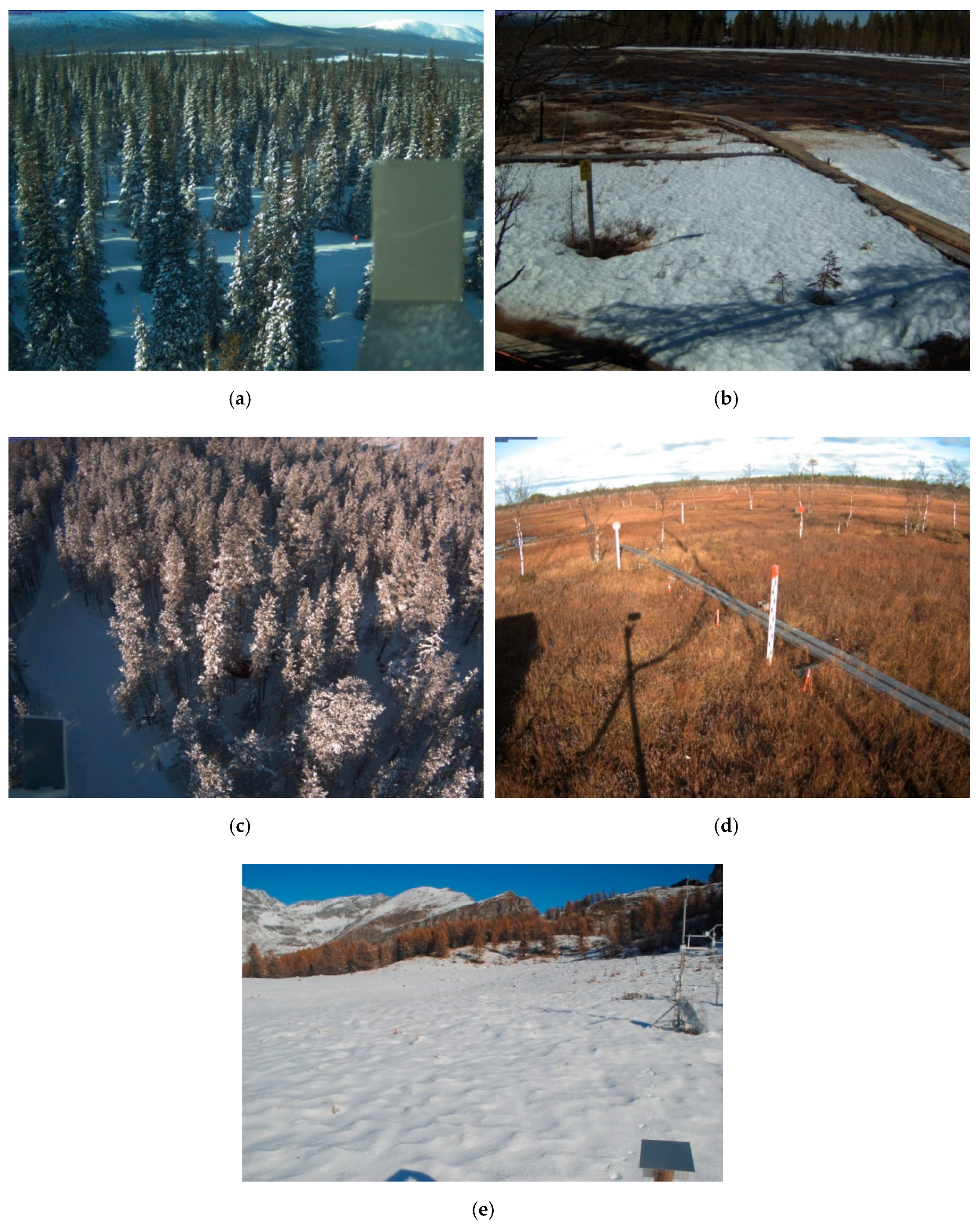
2.3.1. In-Situ Webcam Imagery

In Finland and in Italy, in-situ webcam imagery has been used to assess the consistency of FSC maps based on S-2 data (S-2-derived FSC), which are derived by counting the number of S-2 snow pixels versus the total number of S-2 pixels over the camera FOV. Webcams have been selected according to two main criteria. The first constraint requires a sufficiently wide webcam field of view (FOV) enabling the comparison with S-2-derived FSC. Secondly, webcams providing a properly representative dataset of observations have been primarily selected. With the aim of complying with these conditions, five webcams have been selected (

Table 5. Selected in-situ cameras in Finland and Italy.

Site Name	Coordinates	Camera Brand and Model	Resolution	S-2 Tile	No. of Analyzed Images
Torgnon	45.84° N, 7.57° E	Campbell CC640	0.3 MP	T32TLR	24
Sodankylä peatland	67.37° N, 26.65° E	Stardot Netcam SC	5.0 MP	T35WMQ	22
Sodankylä canopy	67.36° N, 26.64° E	Stardot Netcam SC	5.0 MP		22
Lompolojankka peatland	69.80° N, 24.21° E	Stardot Netcam SC	5.0 MP	T34WFA	23
Kenttärova canopy	67.99° N, 24.24° E	Stardot Netcam SC	5.0 MP		23

), only one of which located over Italian Alps, mainly due to the complex topography, which strongly limits the extent of the webcam FOV.

The four cameras selected in Northern Finland are part of the camera network deployed in the frame of the MONIMET project [24]. MONIMET monitoring network consists of 28 cameras in 14 locations in Finland. The images are free and open. Those cameras produce images at each half an hour during daytime. For the study, midday time images are used since the snow cover does not change significantly during the day. One of the cameras is located in Kenttärova looking over a large evergreen spruce forest, another one is located in Lomppolojankka, a peatland site, and the other two in Sodankylä, located in a Scots pine ecosystem and in a wetland site, respectively. The FOVs of those cameras is shown in Figure 7a–d.

The webcam located in Aosta Valley (north-western Italian Alps) is at the experimental site of Torgnon, which belongs to the Phenocam network [71]. The camera is pointed north and it looks over grassland with mountains visible at distance. Camera images are provided every hour from 10 a.m. to 4 p.m. [21]. The FOV of the camera is shown in Figure 7e.

2.3.2. In-Situ Snow Measurements

In Turkey, binary snow maps derived from S-2 imagery have been validated against ground-based measurements for the winter season 2017/18. Snow data from automatic weather stations (i.e., AWOS: Automated Weather Observing System, and SPA: Snow Pack Analyser) operated by Turkish state meteorological service (TSMS) have been used. Daily snow depth (SD) values have been obtained by processing and filtering the raw data supplied by these stations (e.g., removal of possible false snow detection due to grass). This analysis relies on SD measurements provided by 75 ground stations and 205 S-2 images available between November 2017 and April 2018 over Turkey. The validation has been performed over 25 S-2 tiles and 286 in-situ SD observations have been analyzed. Relative positions of S-2 tiles and the ground stations are shown in Figure 8.

3. Methods

After introducing the retrieval algorithms implemented for the generation of the satellite snow products investigated in this study, the processing of in-situ data and imagery used to validate S-2 observations is described. The methodologies for the S-2-based assessment of H-SAF snow products and the assessment of S-2 imagery against in-situ data are presented and discussed, as well as the evaluation metrics.

3.1. Satellite Retrieval Algorithms

Snow detection can be retrieved from optical imagery through different algorithms, which generally rely on thresholding methods based on channel differences and ratios to exploit the different spectral properties of snow-covered areas with respect to snow-free surfaces and clouds. One of the most commonly-used indices is the normalized difference snow index (NDSI), which is defined as the difference of reflectance observed in a visible band and a shortwave infrared one, divided by the sum if the two reflectance values [72]. Indeed, since snow reflectance is high in the visible wavelengths and low in the shortwave infrared ones, this method enables distinguishing snow from clouds and other non-snow-covered conditions [72,73]. However, it is noteworthy that the suitability of each retrieval algorithm necessarily depends on the main features of the satellite data to be processed [55,74,75].

3.1.1. Sen2Cor Algorithm

S-2 L1C data are downloaded from the Copernicus open access hub. The L1C image product consists of a series of 100 × 100 km²-tiles, each of which is made of thirteen compressed JPEG-2000 images, one for every single band. The MSI TOA reflectance images are processed through the Sen2Cor version 2.5.5, namely the last version of Sentinel-2 L2A prototype processor provided by ESA. Sen2Cor consists of ten main modules and it can perform the tasks of atmospheric, terrain and cirrus correction of L1C input data to generate optimally corrected BOA reflectance images. In this study the L2A_SceneClass (SC) module is used to perform the classification of the input images and to generate Scene Classification (SCL) maps at a spatial resolution of 20 m. The SC algorithm allows the detection of clouds, snow and cloud shadows, and the generation of a classification map consisting of four different classes for clouds (including cirrus), together with six different classifications for shadows, cloud shadows, vegetation, soils/deserts, water and snow (

Table 6. Classes of Sen2Cor SCL map.

Label	Classification
0	No data
1	Saturated/defective
2	Dark area
3	Cloud shadows
4	Vegetation
5	Not vegetated
6	Water
7	Unclassified
8	Cloud (medium probability)
9	Cloud (high probability)
10	Thin cirrus
11	Snow

). The SC module consists of the cloud/snow algorithm, the cirrus detection algorithm, and the cloud showdown detection algorithm to generate the classification map [76]. Each algorithm processes the TOA reflectance input data through a sequence of thresholding filters, which are applied to S-2 spectral bands, band ratios, and indexes. In the cloud/snow detection algorithm, each test provides a cloud probability, which is recursively updated at each step. After thresholding the brightness in the red region of the solar spectrum (band 4), all potentially cloudy pixels are filtered by thresholding the NDSI [72], which is evaluated from spectral bands 3 and 11. Snow confidence map is generated by detecting snow pixels, according to four successive filters using spectral bands 2, 3, 8, 11. Ancillary information on yearly snow climatology is used to define the monthly snow probability of each pixel and to discard possible false snow detections. All potentially snow pixels are then filtered by sequentially thresholding the reflectance in band 8 (NIR) and band 2 (blue), and the ratio between band 2 and band 4 to identify main water bodies. Lastly, possible false cloud detection at the boundaries of snowy regions is removed by performing a brightness test on band 12. Once cloud and snow confidence masks are generated, an optional spatial filter can be applied to reduce possible false cloud detection. The cirrus detection algorithm mainly relies on the reflectance thresholding of band 10, because of the high water vapor absorption in this region [77], and an additional cross check is performed against the probabilistic cloud mask.

3.1.2. H-SAF H10 Algorithms

The distribution of snow cover and the non-uniformity of snow properties are significantly different over mountainous and flat/forested areas, since they strongly depend on the local topography and vegetation cover. Therefore, two distinct stand-alone algorithms are implemented within the product generation and applied according to a mountain mask defined in [56]. The algorithm for flat/forested areas has been developed by Finnish Meteorological Institute (FMI) [70,78]. The algorithm utilizes TOA radiances of six SEVIRI channels (0.635, 0.81, 1.64, 3.90, 10.80, 12.00 µm), the brightness temperatures of three channels (3.90, 10.80, and 12.00 µm), sun and satellite zenith and azimuth angles, the International Geosphere-Biosphere Programme (IGBP) land-cover type by the U.S. Geological Survey (USGS), and the land surface temperature (LST) classification produced by the EUMETSAT’s Satellite Application Facility on Land Surface Analysis (LSA SAF) [77]. While information from channels around 0.635, 0.81, and 1.64 µm are used to classify different surface types [72,79,80], the algorithm exploits the radiance ratio of SEVIRI channels 2 (0.81 µm) and 3 (1.64 µm), and the brightness temperature difference of channels 10 (12.00 µm) and 4 (3.90 µm) to properly detect clouds [81,82]. The Middle East Technical University (METU) developed the algorithm for mountainous areas [56], which exploits 4 SEVIRI spectral channels (0.635 µm, 1.64 µm, 3.90 µm, 10.80 µm). Cloud discrimination is preliminary performed to identify cloud-free pixels by jointly using Cloud Mask (CMa) and Cloud Type (CT) products of the EUMETSAT’s Nowcasting Satellite Application Facility (NWC SAF) [83]. Firstly, pixels having reflectance values higher than 0.35 are collected, because of the high visible reflectance of snow. Secondly, since snow cover has a low reflectance in the middle infrared and a high reflectance in the visible, pixels having snow index (SI) value lower than 0.6 are collected, which is evaluated by dividing channel 3 (1.64 µm) to channel 1 (0.635 µm) [84,85]. Lastly, pixels having temperature lower than 288 K on channel 9 (10.80 µm) are accepted, considering that the temperature of snow cannot exceed the freezing point [86]. It is noteworthy that sun zenith angle (SZA) thresholds are applied, SZA > 80 in the FMI algorithm and SZA > 85 in the METU algorithm are used for discarding the low-illuminated areas. No atmospheric correction is included in both algorithms. The final snow recognition product results from the merging of the products for flat/forested and mountainous areas over the full H-SAF spatial domain.

3.1.3. H-SAF H12 Algorithms

Consistently with H-SAF H10 product, two different retrieval algorithms are separately applied for flat/forested and mountainous areas. Since the observing cycle of satellites over Europe is about 3 h, the scenes are multi-temporally analyzed to search for time instants of cloud-free conditions in 24 h. The retrieval algorithm of FSC in forested/flat areas has been developed at FMI. The method is based on a semi-empirical reflectance model [87], which evaluates the reflectance as a function of the snow-covered area by using visible and near-infrared data (visible band 1) [88]. Since forest transmissivity is of critical importance to estimate the snow-covered area in all conditions of forest coverage, the algorithm relies on the transmissivity map generated from reflectance data acquired at full dry snow cover conditions to guarantee a proper contrast between forest canopy and ground. However, a priori information on forests is not needed, because the effective average forest transmissivity is estimated from Earth observation reflectance data. Conversely, the retrieval algorithm for mountainous areas involves the thresholding of NDSI at 0.4, since it allows the derivation of the resulting average fraction of snow-covered area by retrieving snow and snow-free ground from satellite data according to the reflectance values [55]. Because in mountainous regions the sun zenith and azimuth angles, as well as direction of observation relative to these are the most limiting factors [89], possible terrain effects are properly removed from the measured radiance through a statistical-empirical correction method [90]. Once the visible channel is corrected due to topographic effect, the average reflectance values are determined from pixels of pure snow-covered area and pure bare ground. In defining the pure snow-covered area and snow-free bare ground, the NDSI threshold greater than 0.4 and lower than 0 are used, respectively. The original model has previously been developed by [91]. According to this approach, the pixel reflectance is modelled as a linear mixture of snow, individual tree species and snow-free bare ground (e.g., rock, soil, low vegetation). For mountainous areas the equation considers snow and bare ground, because of the general lack of trees at high altitudes:

$${\overline{R}}_G=A_{SW}{R}_{SW}+A_{BG}{R}_{BG}$$

(1)

where ${\overline{R}}_G$ is the modelled pixel reflectance for a given wavelength, A represents area fractions of a pixel (with $A_{SW}+A_{BG}=1$), R is the reflectance, subscripts SW and BG refer to snow and bare ground, respectively.

It is noteworthy that both atmospheric and topographic corrections are implemented in H12 algorithms. The products for flat/forested and mountainous areas are merged over the full H-SAF area, according to the mountain mask defined in [56]. The merging algorithm is properly designed to minimize the projection errors [92].

3.2. Validation of Sentinel-2 Imagery with In-Situ Data

3.2.1. Validation of Sentinel-2 Imagery by In-Situ Webcams

The validation is based on the comparison of single daily FSC values derived from camera observations to the corresponding single values obtained from S-2-derived FSC maps over the observed area. FSC values have been estimated by experts through the visual inspection of camera images. Visual inspections have been limited over area of interests (AOIs) selected according to both camera properties and the local topographic features, so that the snow cover is clearly visible, and the relative surface area can be estimated as accurately as possible. FSC values have been estimated in 10%-intervals (i.e., 0%, 10%, …, 90%, 100%). The visual inspection of each image has been performed by 4 expert observers. With the aim of assessing the subjective error, the resulting RMSE of FSC estimates has been also calculated, as shown in

Table 7. AOI Sizes, corresponding number of S-2 pixels and subjective error of webcam data observers.

Site Name	AOI Size [m2]	Number of S-2 Pixels	RMSE (All Days)	RMSE (Only Patchy Snow Cover)
Torgnon	1,056,171	2722	13.6%	13.6%
Sodankylä peatland	3976	9	0%	0%
Sodankylä canopy	4760	11	6.3%	13.2%
Lompolojankka peatland	12,310	33	5.7%	15.8%
Kenttärova canopy	254,373	633	0%	0%

. The study of Arslan et al. (2017) [33] has estimated that the subjective error is within 10%, in terms of FSC. For the comparison, average values of the visual estimates have been used to minimize the subjective error.

To properly validate the mapping of S-2-derived FSC, a mask for each selected webcam has been created by drawing polygons over the approximate AOIs using Google Earth. This has been done by visually comparing the landmarks in webcam images and Google Earth optical satellite data overlay. AOIs have been modified according to the landmarks so that the polygons were as accurate as possible. The polygons have been then converted into GeoTIFF files to be used in the FSC evaluation over each AOI from S-2-based snow cover maps (S-2-derived FSC). Area sizes of those polygons and the corresponding number of S-2 pixels are shown in Table 7. The comparison has been performed also over the three AOIs corresponding to relatively low numbers of pixels in S-2 grid, since in those sites most of the images were available either in full snow cover or snowless conditions, which make this analysis feasible. Along with FSC, cloud cover fraction is also calculated for each AOI.

As an example, AOI for the Kenttärova canopy camera and S-2 derived snow cover map over the AOI for 18 February 2018 are shown in Figure 9. In Figure 9c are reported the approximate camera FOV (white polygon) and the selected AOI (yellow polygon) in the Google Earth view. AOI from the camera FOV is reported in Figure 9a,b. The snow cover map derived from the S-2 image over the AOI polygon is shown in Figure 9d. In this example, while experts have estimated FSC as full snow cover (100%) from camera images (at 09:00 and 11:00), S-2-derived FSC (at 10:10) has been estimated as 82%. However, it is noteworthy that 38% of the analysed pixels over the AOI are cloudy or unclassified.

After obtaining the value pairs for the comparison, the ones having cloud cover fraction over 50% have been filtered out. The value pairs of FSC have been compared and the resulting RMSE values have been evaluated.

3.2.2. Validation of Sentinel-2 Imagery against Ground-Based Snow Measurements

The procedure to validate S-2 snow mapping against ground-based data relies on the thresholding of SD measurements to properly define snow and snowless conditions. According to the in-situ measures, the presence of snow is detected whenever a threshold of 5 cm is exceeded. This threshold has been set due to the expected uncertainty in measuring devices [93].

3.3. Procedures of Cross-Sensor Comparison between Satellitesnow Products

After processing S-2 data through Sen2Cor SC module, a quality check of the satellite data series has been performed through random visual inspections to prevent possible systematic inconsistencies. The comparison between observations sensed by different sensors on the same day is performed at the scale of S-2 tile. Indeed, the consistency assessment of H-SAF products against S-2 data is carried out individually over each single tile. In order to properly perform the comparison analysis, all the satellite snow products have been preliminarily re-projected to the same common image projection, namely WGS84/UTM. Since the analysis is tile-based, maps over the geographic extension of each selected S-2 tile are derived from the original full images of both H-SAF products. The selection of the data subset limited over the domain of each tile is carried out by considering the local coordinates of tiles borders, in order to properly guarantee the intersection of the satellite products over each S-2 tile.

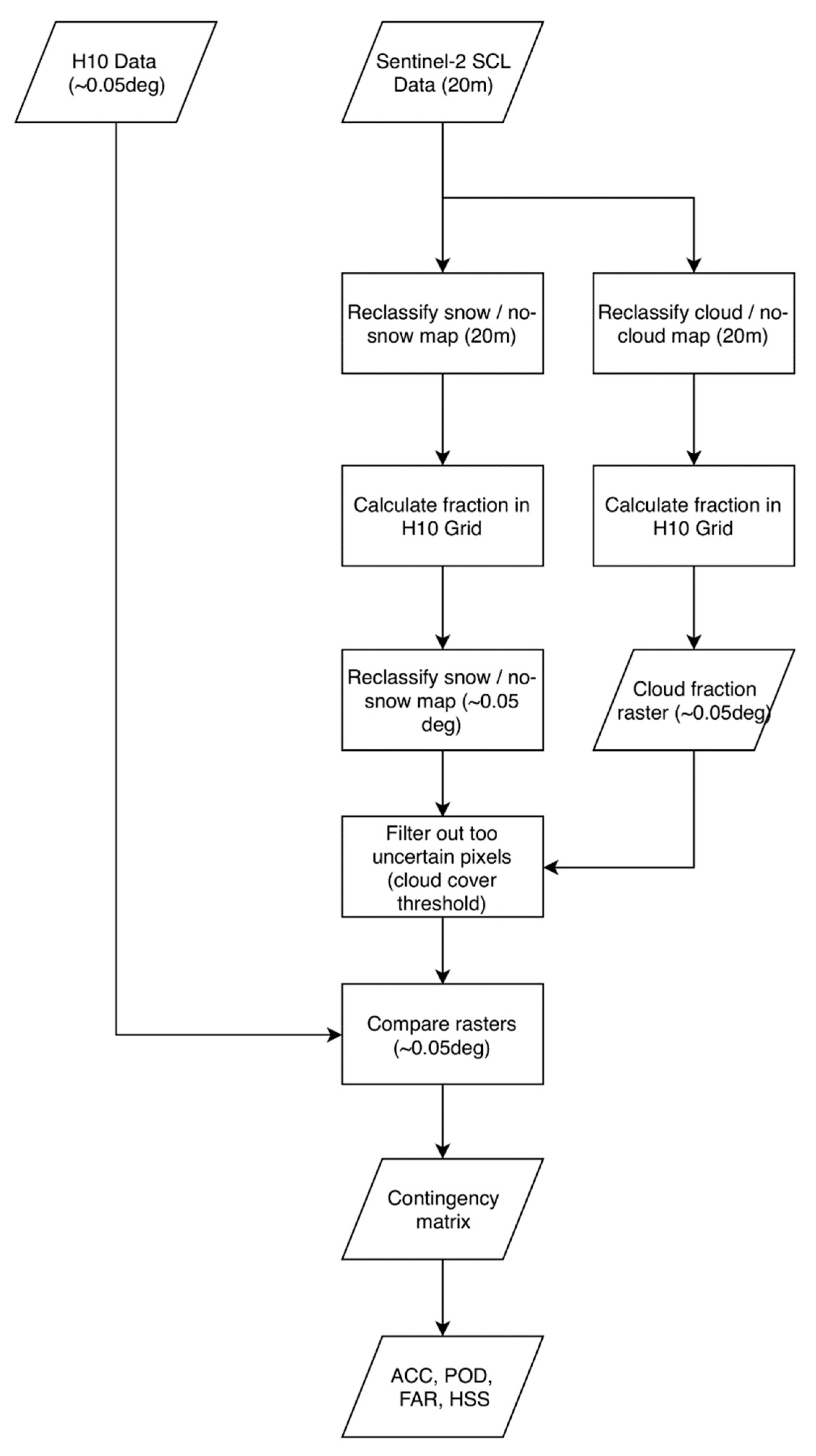
3.3.1. Comparison between Sentinel-Based Snow Masks and H-SAF H10

Figure 10 shows the comparison procedure. Firstly, binary snow masks (presence/absence of snow cover) are derived from both H10 and S-2 SCL maps. According to the original classification of SCL map (Table 6), vegetation, not vegetated, and water (Table 6, classes 4, 5, 6) pixels have been classified as no-snow pixels. Unclassified (Table 6, classes 0, 1, 2, 7) and cloud-contaminated (Table 6, classes 3, 8, 9, 10) pixels are flagged and neglected in the comparison of snow maps, with the aim of preventing possible cloud cover affecting the snow detection [57]. Consistently, H10-based snow masks are derived by considering snow and bare-soil pixels. Since the satellite products are differently gridded, the comparison is performed at the coarser spatial resolution of the H-SAF H10 [55]. For each H10 grid cell, the percentage of snow cover is determined according to the S-2 observations by counting the number of S-2 snow pixels versus the total number of S-2 pixels in the coarser cell [55]. This computation results into an S-2-based FSC map (S-2-derived FSC). In order to restore a binary snow mask, each resulting S-2-based coarse cell is then classified as snow if FSC is higher than 50%, otherwise it is classified as soil [57,94]. S-2-based coarse cell where more than the 50% of fine S-2 pixels are classified as cloud or unclassified are neglected in order not to compromise the analysis results. A preliminary analysis has been performed by testing threshold values equal to 25%, 50%, 75% to properly assess the impact of the thresholding of cloud cover at pixel scale. The results have revealed a poor sensitivity of the comparison procedure to the threshold value.

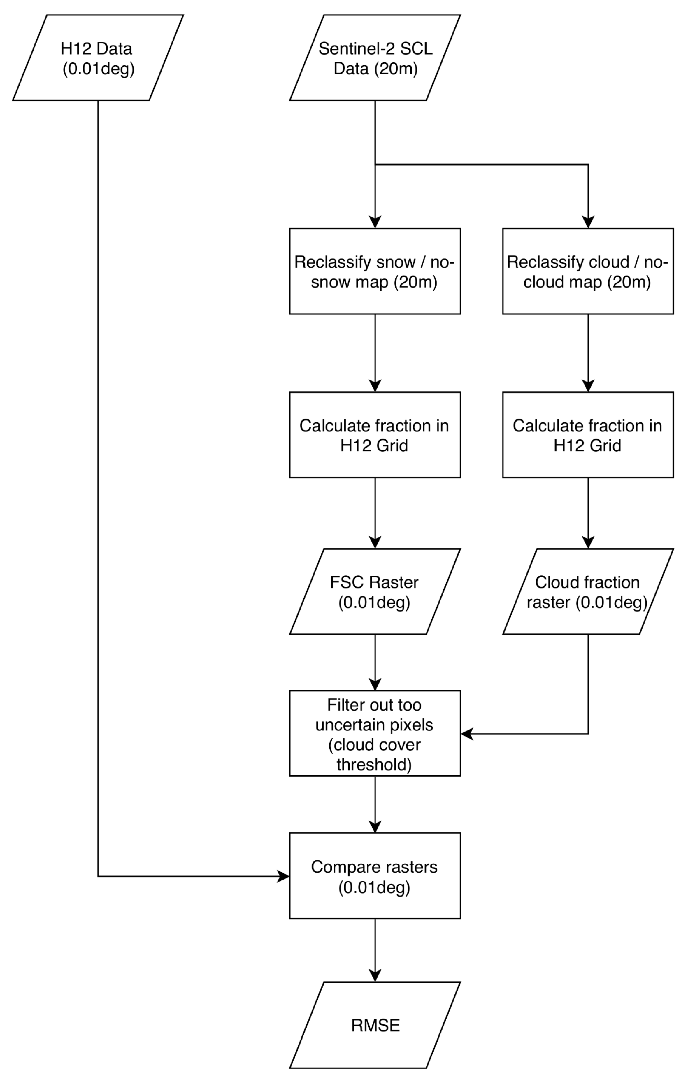
3.3.2. Comparison between Sentinel-Derived FSC Maps and H-SAF H12

Consistently with the assessment of H-SAF H10 product, the analysis of H12 data relies on the same procedure and assumptions. The only main difference is the lack of the thresholding of FSC derived from S-2 imagery over the coarser H-SAF grid (S-2-derived FSC), since it is directly comparable with H12 product. Indeed, this analysis compares FSC maps of H12 product, which are generated through retrieval algorithms (Section 3.1.3), with the S-2-based FSC maps, which are derived by counting the number of S-2 snow pixels versus the total number of S-2 pixels in the coarser H12 cell. The comparison scheme is reported in Figure 11.

It is noteworthy that when mapping the snow cover through remotely-sensed optical imagery, forests constitute a challenge, since the canopy (1) partially obscures the signal along the path from ground to sensor and, (2) alters the observed reflectance [87]. Therefore, the accuracy of snow mapping generally decreases in forested areas with respect to non-forested regions [72,95,96]. Even though several methodologies have been proposed for the detection of snow under forest canopy [87,91,96,97,98,99,100], this issue still remains a critical research topic. Subpixel classification methods [87,101,102] are used to generate FSC maps with the aim of overcoming the limitations related to mixed-pixels problem affecting coarse-resolution imagery, namely possible mixtures of land cover classes (i.e., snow, soil, rock, vegetation, water, etc.) and area fractions of different cover classes within a pixel.

When assessing the consistency between S-2 and H12 data, the impact of vegetation on snow detection need to be investigated. Indeed, since the H12 retrieval algorithm in flat/forested area involves transmissivity maps, this product results from snow detection at ground level. Conversely, S-2 snow mask is derived from snow detection on canopy and thus it can be hindered by the presence of vegetation, mainly where forest cover is present. It is noteworthy that this difference in retrieval algorithms is supposed not to affect the analysis shortly after snowfall events, when forested areas are likely to be classified as snow pixels because of canopy interception [103]. On the other hand, during periods when no snowfall event occurs, the comparison between the two snow products can be more challenging. Indeed, especially in dense forests, the lack of intercepted snow can lead to a misleading S-2 classification as snow-free surface despite the presence of snow cover under canopy. Therefore, with the aim of addressing this critical issue, a further analysis has been performed according to the information on different vegetation types supplied by ESA GlobCover 2009 land cover map. The impact of the vegetation cover has been investigated throughout the whole analysis period by considering a sample of one tile in each country. The comparison between S-2-derived FSC and H12 product has been performed after preliminarily filtering out of the vegetated pixels in S-2 data by using the information supplied by GlobCover data for flat areas and without filtering in mountainous regions. For the filtering, S-2 derived FSC maps have been collocated with the GlobCover map. The pixels corresponding to flat regions in the mountain mask and belonging to the vegetation class V1 in GlobCover (described in Section 2.2) have been discarded from S-2 derived FSC maps. After that, the comparison has been performed through the same algorithm previously described. This procedure has also been applied for the vegetation class V2 to properly assess the impact of different vegetation types on snow detection. Results are presented separately for both classes.

3.4. Evaluation Metrics

For the consistency assessment of the mapping of snow extent, a contingency table is evaluated (

Table 8. Contingency table reporting number of HITS (a), number of FALSE ALARMS (b), number of MISSES (c), number of CORRECT NEGATIVES (d).

		Reference Dataset
		Snow	No Snow
Analyzed dataset	Snow	a	b
	No Snow	c	d

).

From these classification results, different scores for dichotomous statistics are evaluated:

● Probability of detection:

POD = a/(a + c)

(2)

● False alarm ratio:

FAR = b/(a + b)

(3)

● Probability of false detection:

POFD = b/(b + d)

(4)

● Accuracy:

ACC = (a + d)/(a + b + c + d)

(5)

● Critical success index:

CSI = a/(a + b + c)

(6)

● Heidke skill score:

HSS = 2(ad − bc)/[(a + c)(c + d) + (a + b)(b + d)]

(7)

FSC is assessed through the evaluation of Root Mean Square Error (RMSE) with respect to the reference dataset $\left(FS{C}_{ref}\right)$.

$$\mathrm{RMSE}=\sqrt{\frac{{{\displaystyle \sum }}_{i=1}^n{\left(FS{C}_{ref,i}-FS{C}_i\right)}^2}{n}}$$

(8)

4. Results and Discussion

4.1. Validation of Sentinel-2 Imagery

When validating S-2 imagery against in-situ observations, it is noteworthy that the evaluation metrics have been evaluated by considering ground-based datasets as the reference ones.

4.1.1. In-Situ Digital Imagery

The comparison relies on a total of 50 pairs of FSC values, resulting from the analysis of matching webcam and S-2 images, both in Finland and in Italy. The evaluation has revealed a total RMSE value of 12.22%. In overall, S-2 snow mapping reveals a general FSC overestimation. When neglecting full-snow and bare-soil classification (i.e., FSC equal to 0% and 100%), the total RMSE value increases up to 19.82% for 19 value pairs. It is noteworthy that no outlier affects the distribution and the analyzed data boast a high correlation. Figure 12 shows the data scatterplot resulting from the comparison.

The undesired cases resulting in high errors have been investigated in more detail. In Torgnon, where the AOI is selected over the mountainous area, the three scenes having the highest error are those affected by the largest cloud cover fraction, greater than 29%. Indeed, in the presence of patchy snow cover, partial cloud cover over the area is likely to unavoidably affect the FSC derived from S-2 data. Under conditions of patchy snow cover, S-2 data are affected by overestimation in Lompolojankka. Two occurrences are during the melting period, where the ground is mostly cover by meltwater. One further occurrence is in early winter, where snow cover is still not full and sparse vegetation is likely to hinder the visual inspection.

4.1.2. Ground-Based Snow Measurements

The validation of S-2 snow mapping against ground-based SD measurements in Turkey has revealed a significant consistency of satellite imagery, as evidenced by the highest number of hits and lower values of false alarms and misses (

Table 9. Contingency table of ground-based validation of S-2 binary snow maps in Turkey for winter season 2017/18.

		Ground-Based Measures
		SD ≥ 5 cm	SD < 5 cm
S-2 Binary Snow Masks	Snow	201	17
	No Snow	43	25

).

As shown in

Table 10. Evaluation metrics of ground-based validation of S-2 binary snow maps in Turkey for winter season 2017/18.

Metrics	Value
POD	0.82
FAR	0.08
POFD	0.40
ACC	0.79
CSI	0.77
HSS	0.33

reporting the resulting evaluation metrics, the remotely-sensed high-resolution observations properly succeed in detecting the presence of snow cover.

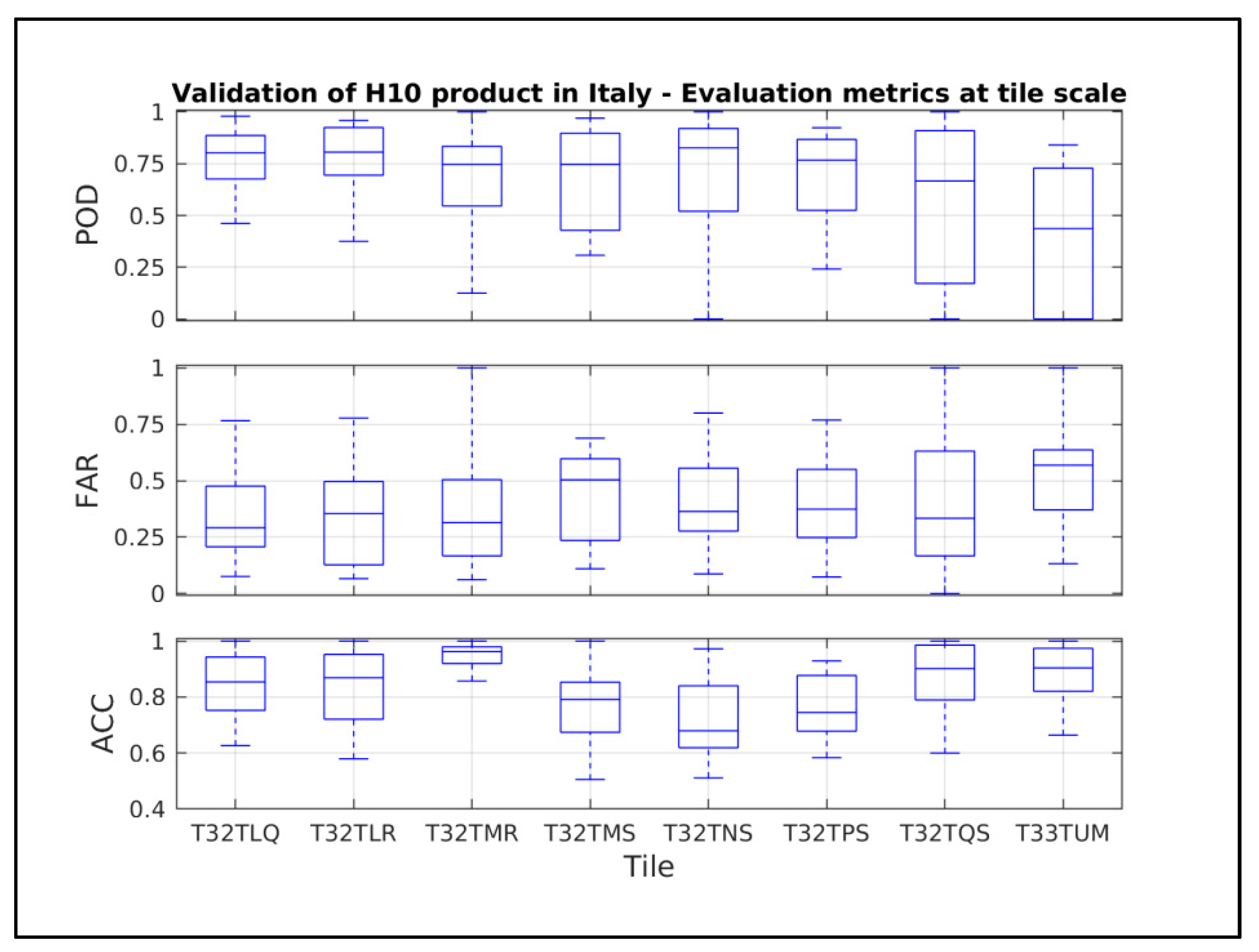
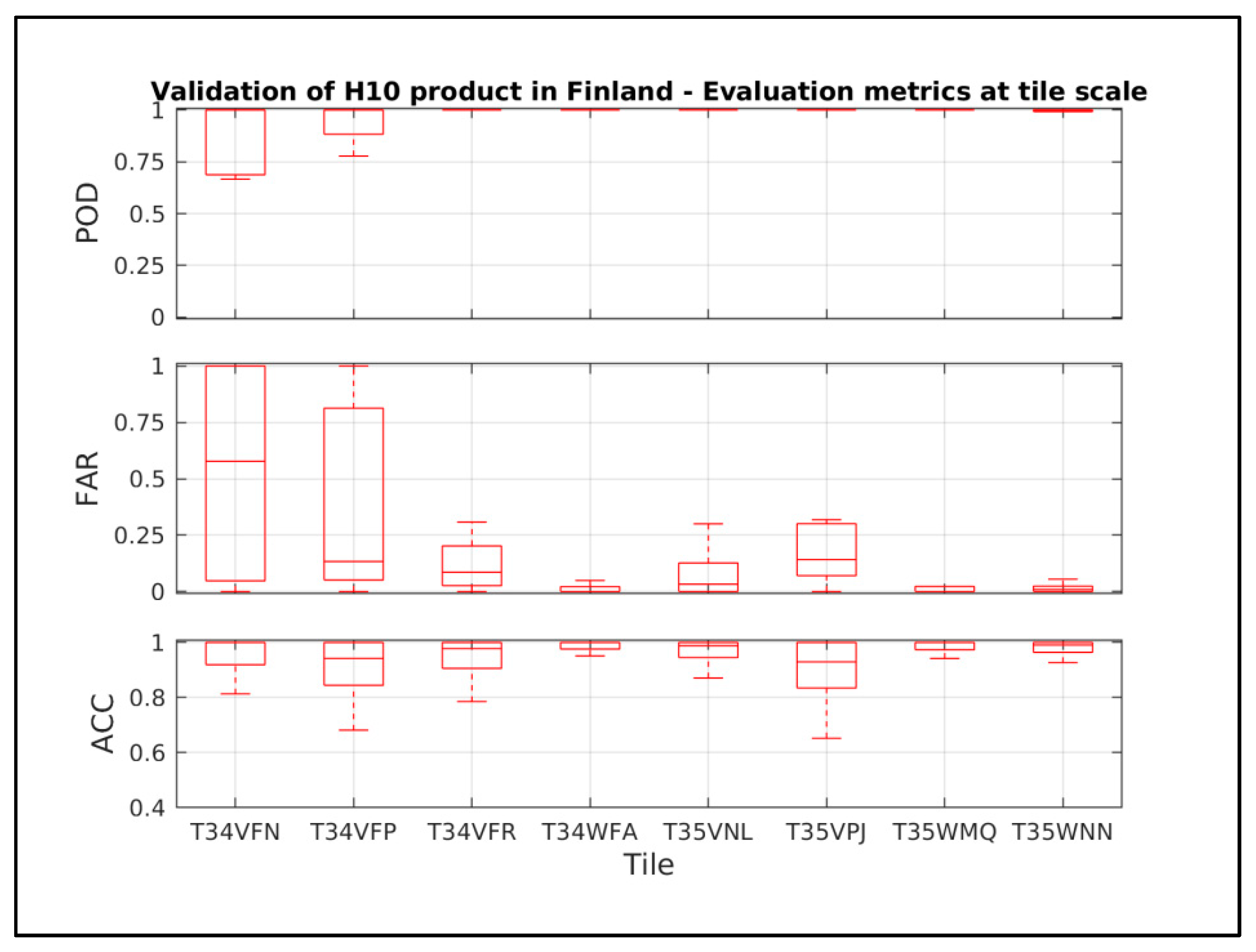
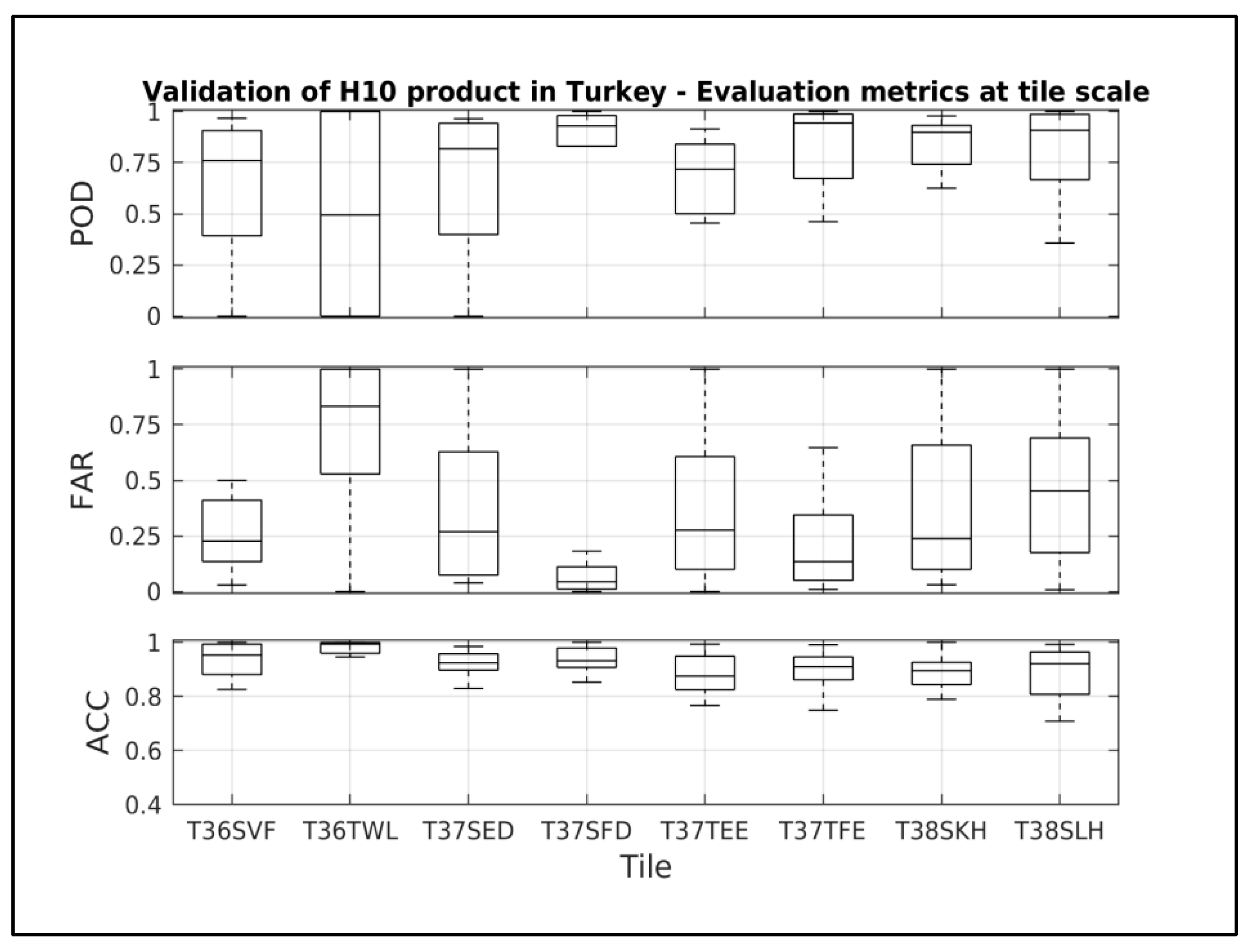
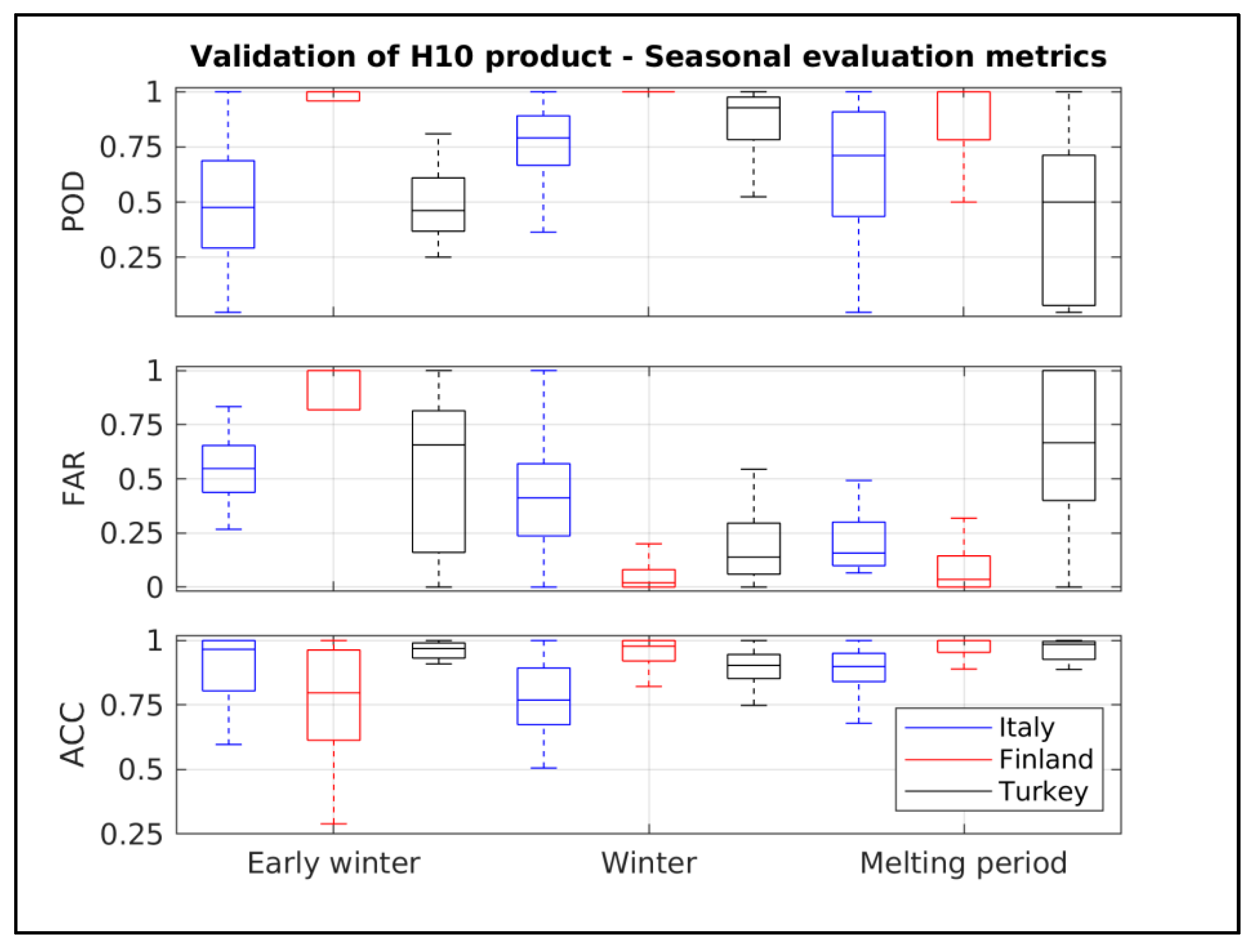
4.2. Cross-Sensor Comparison of Snow Extent Products

For each S-2 tile a pixel-to-pixel analysis has been performed to evaluate the consistency between the S-2-based maps of snow extent and H-SAF H10 product.

Figure 13, Figure 14 and Figure 15 show the comparison results in terms of POD, FAR and ACC for each analyzed tile in Italy, Finland and Turkey, respectively. When assessing the evaluation metrics, it is noteworthy that H10 product generally reveals higher performances over flat areas (i.e., Finland), rather than over mountainous regions (i.e., Italian Alps and Turkey). This issue is mainly due to the impact of the local complex topography affecting the sensors capability to detect snow. Indeed, mapping the high spatial variability of snow cover distribution over mountain sides is a challenging task at the coarser satellite resolution. Conversely, when considering the vegetation cover of each pixel (Table 3), even the presence of the vegetation species supposed to hinder the snow detection (e.g., evergreen needle-leaved forest) results in a lesser impact than topographic factors. However, both in Italy and Turkey, H10 product reveals a slightly weaker reliability over the most vegetated tiles, namely T32TQS and T33TUM, and T36TWL, respectively. This result suggests that the vegetation has a greater impact where the local topography is complex, due to overlapping effects. Nevertheless, H10 product generally ensures an accuracy greater than 0.8, except for tiles T32TNS and T33TPS over Italian Alps.

With the aim of investigating whether product performances are affected by the seasonality of snow cover, the evaluation metrics have been assessed under different snow cover conditions. Indeed, three different periods have been individually assessed, namely early winter (i.e., October and November), winter (i.e., December-March), melting period (i.e., April and May) (Figure 16).

Consistently with the tile-scale analysis, the agreement between S-2 and H10 data is higher over flat areas (i.e., in Finland). The analyses show that in early winter the lower accuracy and higher FAR values of H10 product over flat areas are mainly due to frequent cloudiness, which is likely to affect the snow detection. However, it is noteworthy that the presence of canopy is likely to have a higher impact during early winter and melting period. Indeed, in those months, the presence of patchy snow cover and the lower frequency of snowfall events intercepted by canopy make the snow mapping more challenging, especially where dense forests are present. Furthermore, it is important to consider that the 50%-thresholding of FSC derived from S-2 data (Section 3.2) is likely to affect the analysis mainly during the transition periods, when patchy snow cover is present.

The higher consistency between H10 product and S-2 snow masks over flat areas is confirmed when assessing the evaluation metrics throughout the whole analysis period (

Table 11. Comparison between S-2-based snow masks and H10 product—Median values of evaluation metrics throughout the whole analysis period. H10 product requirements for both flat/forested (i.e., Finland) and mountainous areas (i.e., Italian Alps, Turkey) (POD_thr and FAR_thr) are reported [104].

Area	PODthr	FARthr	POD	FAR	POFD	ACC	CSI	HSS
Finland	0.80	0.20	0.98	0.10	0.07	0.95	0.89	0.90
Italian Alps	0.60	0.30	0.78	0.35	0.16	0.83	0.55	0.59
Turkey			0.91	0.13	0.08	0.92	0.80	0.83

). While H10 product reveals satisfying evaluation metrics of the same ranges in Finland and in Turkey, the Alpine complex topography strongly affects the snow mapping over this region, as proved by the poorer scores.

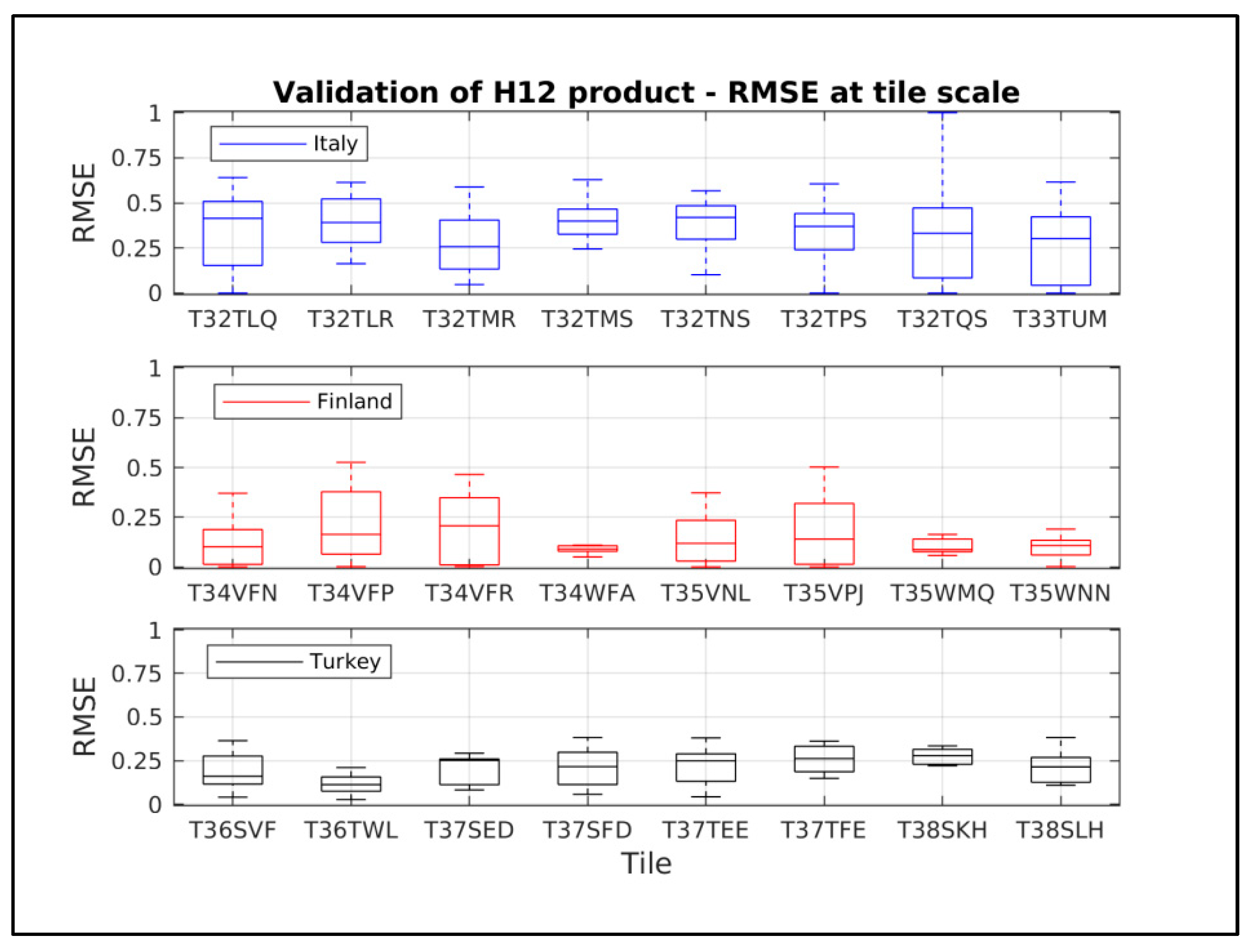
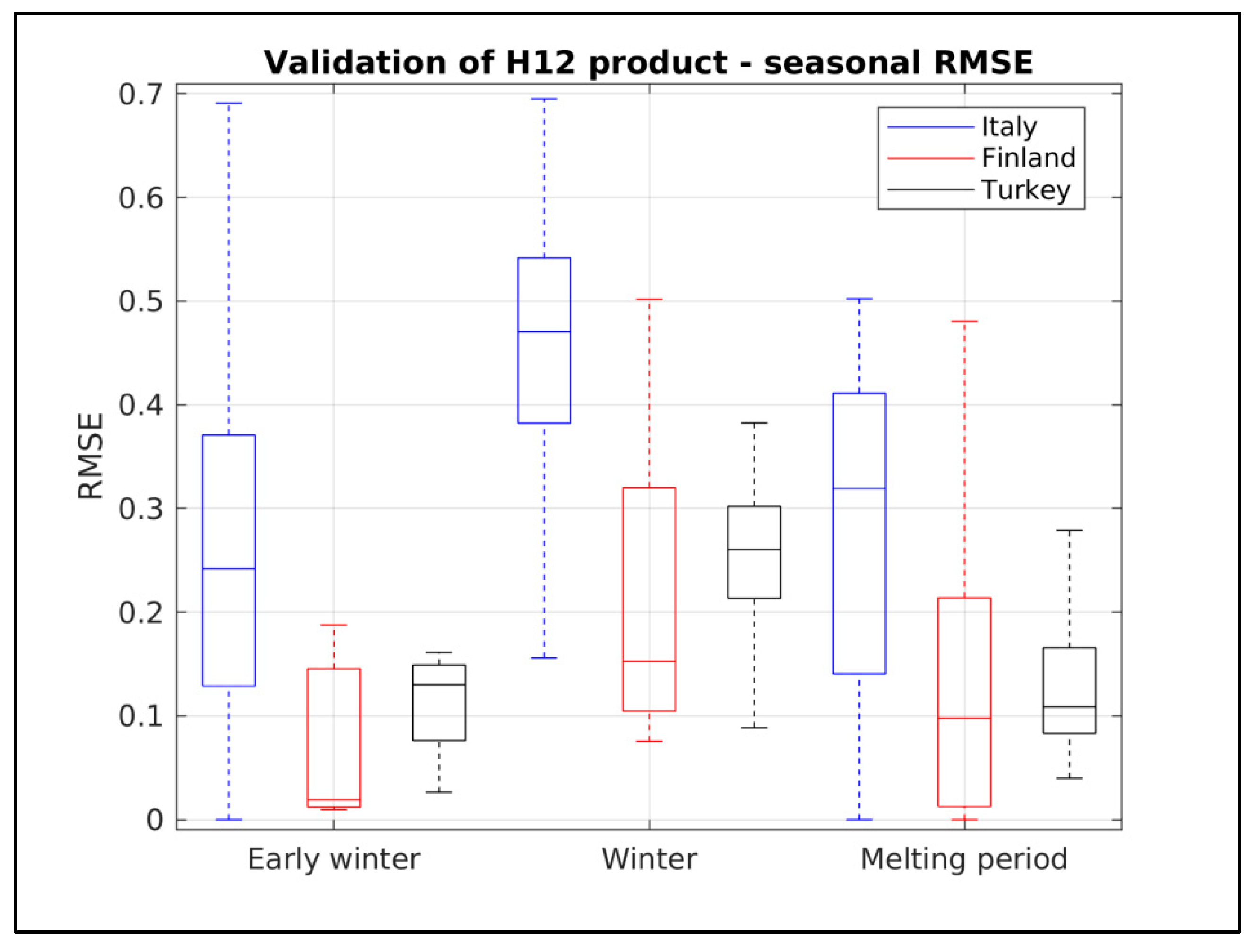
4.3. Cross-Sensor Comparison of Effective Snow Cover Products

The agreement between the mapping of the FSC derived from S-2 imagery and H12 product has been assessed according to the same pixel-to-pixel approach.

Like in the assessment of H10 data, the complex topography in mountainous areas affects the consistency between the two analyzed datasets, especially over the Italian Alps, where RMSE values are higher than the other case studies (Figure 17). However, RMSE scores are generally lower than 0.4, except for the same tiles in Italy, in compliance with the product requirements [105].

Figure 18 shows that during the winter period RMSE values are generally higher than in other seasons. This issue is mainly due to overestimated classifications as full snow cover over the coarser spatial resolution of H12 product with respect to that derived from 20-m S-2 imagery, especially in mountainous regions.

The RMSE assessment over the whole analysis period confirms higher performances of H12 product over flat areas (i.e., Finland) than in mountainous regions (i.e., Italian Alps and Turkey) (

Table 12. Overall RMSE values for the comparison between S-2-derived FSC maps and H12 product. H12 product requirement for both flat (i.e., Finland) and mountainous areas (i.e., Italian Alps, Turkey) (RMSE_thr) is reported [105].

Region	RMSEthr	RMSE
Finland	0.40	0.15
Italian Alps	0.50	0.33
Turkey		0.21

). However, the product target requirements [105] are generally satisfied over both mountainous (RMSE ~ 30%) and flat (RMSE ~ 20%) areas.

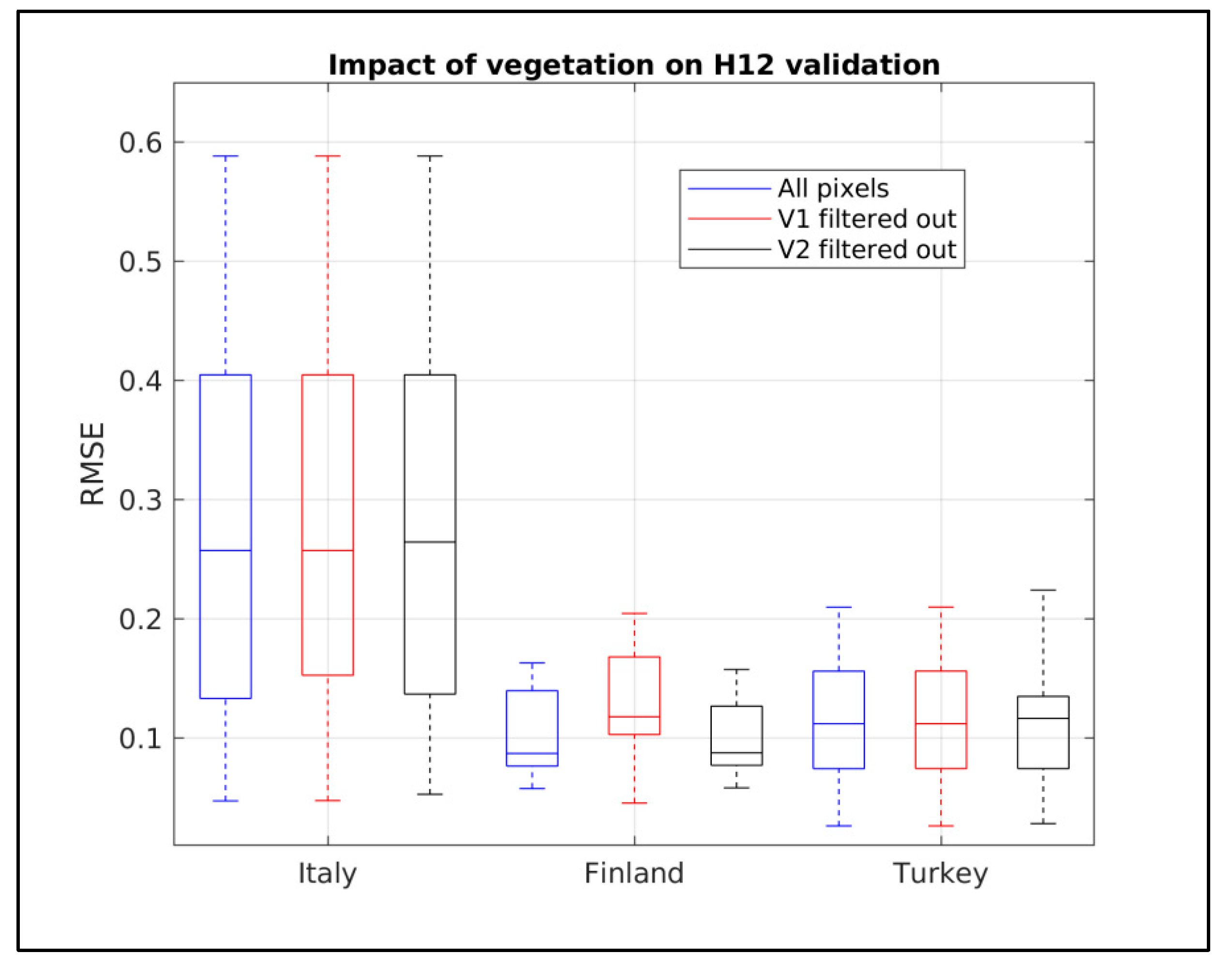
Impact of Vegetation on Snow Detection

In order to properly assess the impact of the vegetation cover within the assessment of H12 product, the results obtained by filtering out the main classes V1 and V2 are individually evaluated against the reference ones relying on all S-2 pixels. As expected, the vegetation cover has a negligible impact on the comparison results in the Alpine region, since H12 and S-2 snow retrieval algorithms are consistent over the mountain mask (Section 3.2.2). Conversely, in Finland and Turkey the comparison procedure reveals a slight sensitivity to the different vegetation classes. While the snow detection is more affected by V1-vegetation class (i.e., needle-leaved evergreen forest) in Finland, V2-vegetation class (i.e., broadleaved deciduous forest) has a higher impact in Turkey. Figure 19 shows that by filtering out V1-vegetation pixels, the RMSE value in Finland increases with respect to the all-pixels analysis. The reduction in consistency between H12 and S-2 snow mapping suggests a good agreement of the two datasets over dense forests mainly due to the long-lasting snow interception over canopy during the winter season. Consistently, in Turkey the resulting RMSE slightly increases when filtering V2-vegetation pixels.

5. Conclusions

This study investigated the potential of using S-2 data to assess moderate-resolution EUMETSAT H-SAF product of snow extent (H10) and FSC (H12) in Finland, the Italian Alps and Turkey. Snow masks derived from S-2 imagery have revealed a significant consistency with both ground-based snow measurements (POD = 0.82, FAR = 0.08,) and in-situ webcam photography, revealing a RMSE of about 12%, in terms of FSC. Hence the reliability of assuming this high-resolution dataset as a reference for intercomparison purposes. The results obtained in this study reveal that S-2 data can be properly used to continuously assess these medium resolution satellite snow products, which have been commonly validated against in-situ data so far [53,56]. However, it is noteworthy to consider that under specific conditions the snow mapping derived from S-2 data can be affected by critical flaws. Indeed, the analysis of camera images in the Italian Alps has shown that dense cloud cover can undermine the reliability of S-2 snow masks, mainly when patchy snow cover is present. Furthermore, during melting period the widespread presence of meltwater over flat areas may lead to an overestimation of snow cover.

The results of the cross-sensor comparison prove that the analyzed H-SAF snow products are highly consistent with S-2 imagery in detecting snow, also in terms of FSC, generally in compliance with the products requirements [104,105]. Nevertheless, the analyzed satellite datasets generally reveal a higher agreement over flat/forested areas (POD_H10 and RMSE_H12 equal to 0.98 and 0.15, respectively) than in mountainous regions (over Italian Alps, POD_H10 and RMSE_H12 equal to 0.78 and 0.33, respectively). Indeed, the local complex topography is likely to significantly hinder snow detection over mountain sides at coarser satellite spatial resolution. Conversely, the vegetation cover has turned out to have a less relevant impact on the consistency among remotely-sensed observations, even in the presence of dense evergreen forest. In Finland the long-lasting snow interception on vegetation canopy is expected to contribute to strengthening the agreement between S-2 snow maps and H12 images during the winter season. However, further key issues need to be addressed in the future. Primarily, a comparative study on different retrieval algorithms would allow an assessment of the reliability of the snow mapping derived from S-2 imagery. Secondly, the impact of cloudiness on the consistency among remotely-sensed observations should be investigated in more details through the analysis of scenes with different cloud cover percentages.

Nevertheless, these promising results currently encourage the effective use of the analyzed H-SAF snow products for hydrological and climatological studies, since they provide reliable snow-related information at large scale. Furthermore, thanks to their free availability at a daily scale, both H10 and H12 products are recommended as particularly suited for operational applications.

References

1. Bates, B.; Kundzewicz, Z.; Wu, S. Climate Change and Water; Intergovernmental Panel on Climate Change Secretariat: Geneva, Switzerland, 2008. [Google Scholar]
2. Appel, I. Uncertainty in satellite remote sensing of snow fraction for water resources management. Front. Earth Sci. 2018, 12, 711–727. [Google Scholar] [CrossRef]
3. Thirel, G.; Salamon, P.; Burek, P.; Kalas, M. Assimilation of MODIS snow cover area data in a distributed hydrological model using the particle filter. Remote Sens. 2013, 5, 5825–5850. [Google Scholar] [CrossRef]
4. Kumar, S.V.; Peters-Lidard, C.D.; Arsenault, K.R.; Getirana, A.; Mocko, D.; Liu, Y. Quantifying the added value of snow cover area observations in passive microwave snow depth data assimilation. J. Hydrometeorol. 2015, 16, 1736–1741. [Google Scholar] [CrossRef]
5. Aalstad, K.; Westermann, S.; Schuler, T.V.; Boike, J.; Bertino, L. Ensemble-based assimilation of fractional snow-covered area satellite retrievals to estimate the snow distribution at Arctic sites. Cryosphere 2018, 12, 247–270. [Google Scholar] [CrossRef] [Green Version]
6. Pirazzini, R.; Leppänen, L.; Picard, G.; Lopez-Moreno, J.I.; Marty, C.; Macelloni, G.; Kontu, A.; von Lerber, A.; Tanis, C.M.; Schneebeli, M.; et al. European In-Situ Snow Measurements: Practices and Purposes. Sensors 2018, 18, 2016. [Google Scholar] [CrossRef] [PubMed]
7. López-Moreno, J.I.; Nogués-Bravo, D. A generalized additive model for the spatial distribution of snowpack in the Spanish Pyrenees. Hydrol. Process. 2005, 19, 3167–3176. [Google Scholar] [CrossRef] [Green Version]
8. Bormann, K.J.; Westra, S.; Evans, J.P.; McCabe, M.F. Spatial and temporal variability in seasonal snow density. J. Hydrol. 2013, 484, 63–73. [Google Scholar] [CrossRef]
9. Luce, C.H.; Lopez-Burgos, V.; Holden, Z. Sensitivity of snowpack storage to precipitation and temperature using spatial and temporal analog models. Water Resour. Res. 2014, 50, 9447–9462. [Google Scholar] [CrossRef] [Green Version]
10. Rice, R.; Bales, R.C.; Painter, T.H.; Dozier, J. Snow water equivalent along elevation gradients in the Merced and Tuolumne River basins of the Sierra Nevada. Water Resour. Res. 2011, 47. [Google Scholar] [CrossRef] [Green Version]
11. Molotch, N.P.; Meromy, L. Physiographic and climatic controls on snow cover persistence in the Sierra Nevada Mountains. Hydrol. Process. 2014, 28, 4573–4586. [Google Scholar] [CrossRef]
12. Revuelto, J.; López-Moreno, J.I.; Azorin-Molina, C.; Vicente-Serrano, S.M. Topographic control of snowpack distribution in a small catchment in the central Spanish Pyrenees: Intra-and inter-annual persistence. Cryosphere 2014, 8, 1989–2006. [Google Scholar] [CrossRef]
13. Harpold, A.A.; Guo, Q.; Molotch, N.; Brooks, P.D.; Bales, R.; Fernandez-Diaz, J.C.; Musselman, K.N.; Swetnam, T.L.; Kirchner, P.; Meadows, M.W.; et al. LiDAR-derived snowpack data sets from mixed conifer forests across the Western United States. Water Resour. Res. 2014, 50, 2749–2755. [Google Scholar] [CrossRef] [Green Version]
14. Szczypta, C.; Gascoin, S.; Houet, T.; Hagolle, O.; Dejoux, J.F.; Vigneau, C.; Fanise, P. Impact of climate and land cover changes on snow cover in a small Pyrenean catchment. J. Hydrol. 2015, 521, 84–99. [Google Scholar] [CrossRef] [Green Version]
15. Fayad, A.; Gascoin, S.; Faour, G.; López-Moreno, J.I.; Drapeau, L.; Le Page, M.; Escadafal, R. Snow hydrology in Mediterranean mountain regions: A review. J. Hydrol. 2017, 551, 374–396. [Google Scholar] [CrossRef]
16. Gascoin, S.; Lhermitte, S.; Kinnard, C.; Bortels, K.; Liston, G.E. Wind effects on snow cover in Pascua-Lama, Dry Andes of Chile. Adv. Water Resour. 2013, 55, 25–39. [Google Scholar] [CrossRef] [Green Version]
17. Vionnet, V.; Martin, E.; Masson, V.; Guyomarc’h, G.; Bouvet, F.N.; Prokop, A.; Durand, Y.; Lac, C. Simulation of wind-induced snow transport and sublimation in alpine terrain using a fully coupled snowpack/atmosphere model. Cryosphere 2014, 8, 395–415. [Google Scholar] [CrossRef] [Green Version]
18. López-Moreno, J.I.; Fassnacht, S.R.; Heath, J.T.; Musselman, K.N.; Revuelto, J.; Latron, J.; Morán-Tejeda, E.; Jonas, T. Small scale spatial variability of snow density and depth over complex alpine terrain: Implications for estimating snow water equivalent. Adv. Water Resour. 2013, 55, 40–52. [Google Scholar] [CrossRef] [Green Version]
19. Raleigh, M.; Livneh, B.; Lapo, K.; Lundquist, J. How does availability of meteorological forcing data impact physically-based snowpack simulations? J. Hydrometeorol. 2016, 17, 99–120. [Google Scholar] [CrossRef]
20. Viviroli, D.; Archer, D.R.; Buytaert, W.; Fowler, H.J.; Greenwood, G.; Hamlet, A.F.; Huang, Y.; Koboltschnig, G.; Litaor, M.I.; López-Moreno, J.I. Climate change and mountain water resources: Overview and recommendations for research, management and policy. Hydrol. Earth Syst. Sci. 2011, 15, 471–504. [Google Scholar] [CrossRef]
21. Migliavacca, M.; Galvagno, M.; Cremonese, E.; Rossini, M.; Meroni, M.; Sonnentag, O.; Cogliati, S.; Manca, G.; Diotri, F.; Busetto, L.; et al. Using digital repeat photography and eddy covariance data to model grassland phenology and photosynthetic CO2 uptake. Agric. For. Meteorol. 2011, 151, 1325–1337. [Google Scholar] [CrossRef]
22. Filippa, G.; Cremonese, E.; Migliavacca, M.; Galvagno, M.; Forkel, M.; Wingate, L.; Tomelleri, E.; di Cella, U.M.; Richardson, A.D. Phenopix: AR package for image-based vegetation phenology. Agric. For. Meteorol. 2016, 220, 141–150. [Google Scholar] [CrossRef]
23. Linkosalmi, M.; Aurela, M.; Tuovinen, J.-P.; Peltoniemi, M.; Tanis, C.M.; Arslan, A.N.; Kolari, P.; Aalto, T.; Rainne, J.; Laurila, T. Digital photography for assessing vegetation phenology in two contrasting northern ecosystems. Geosci. Instrum. Methods Data Syst. 2016, 5, 417–426. [Google Scholar] [CrossRef]
24. Peltoniemi, M.; Aurela, M.; Böttcher, K.; Kolari, P.; Loehr, J.; Karhu, J.; Linkosalmi, M.; Tanis, C.M.; Tuovinen, J.-P.; Arslan, A.N. Webcam network and image database for studies of phenological changes of vegetation and snow cover in Finland, image time series from 2014 to 2016. Earth Syst. Sci. Data 2018, 10, 173–184. [Google Scholar] [CrossRef] [Green Version]
25. Peltoniemi, M.; Aurela, M.; Böttcher, K.; Kolari, P.; Loehr, J.; Hokkanen, T.; Karhu, J.; Linkosalmi, M.; Tanis, C.M.; Metsämäki, S.; et al. Networked web-cameras monitor congruent seasonal development of birches with phenological field observations. Agric. For. Meteorol. 2018, 249, 335–347. [Google Scholar] [CrossRef]
26. Wingate, L.; Ogée, J.; Cremonese, E.; Filippa, G.; Mizunuma, T.; Migliavacca, M.; Moisy, C.; Wilkinson, M.; Moureaux, C.; Wohlfahrt, G.; et al. Interpreting canopy development and physiology using the EUROPhen camera network at flux sites. Biogeosci. Discuss. 2015, 12, 5995–6015. [Google Scholar] [CrossRef]
27. Richardson, A.D.; Hufkens, K.; Milliman, T.; Aubrecht, D.M.; Chen, M.; Gray, J.M.; Johnston, M.R.; Keenan, T.F.; Klosterman, S.T.; Kosmala, M.; et al. PhenoCam Dataset v1. 0: Vegetation Phenology from Digital Camera Imagery, 2000–2015; ORNL DAAC: Oak Ridge, TN, USA, 2017.
28. Farinotti, D.; Magnusson, J.; Huss, M.; Bauder, A. Snow accumulation distribution inferred from time-lapse photography and simple modelling. Hydrol. Process. 2010, 24, 2087–2097. [Google Scholar] [CrossRef]
29. Salvatori, R.; Plini, P.; Giusto, M.; Valt, M.; Salzano, R.; Montagnoli, M.; Cagnati, A.; Crepaz, G.; Sigismondi, D. Snow cover monitoring with images from digital camera systems. Ital. J. Remote Sens. 2011, 43, 137–145. [Google Scholar] [CrossRef]
30. Bernard, É.; Friedt, J.M.; Tolle, F.; Griselin, M.; Martin, G.; Laffly, D.; Marlin, C. Monitoring seasonal snow dynamics using ground based high resolution photography (Austre Lovenbreen, Svalbard, 79 N). ISPRS J. Photogramm. Remote Sens. 2013, 75, 92–100. [Google Scholar] [CrossRef]
31. Garvelmann, J.; Pohl, S.; Weiler, M. From observation to the quantification of snow processes with a time-lapse camera network. Hydrol. Earth Syst. Sci. 2013, 17, 1415–1429. [Google Scholar] [CrossRef] [Green Version]
32. Härer, S.; Bernhardt, M.; Corripio, J.G.; Schulz, K. PRACTISE-Photo Rectification and ClassificaTIon SoftwarE (V. 1.0). Geosci. Model Dev. 2013, 9, 307–321. [Google Scholar] [CrossRef]
33. Arslan, A.N.; Tanis, C.M.; Metsämäki, S.; Aurela, M.; Böttcher, K.; Linkosalmi, M.; Peltoniemi, M. Automated Webcam Monitoring of Fractional Snow Cover in Northern Boreal Conditions. Geosciences 2017, 7, 55. [Google Scholar] [CrossRef]
34. Tanis, C.; Peltoniemi, M.; Linkosalmi, M.; Aurela, M.; Böttcher, K.; Manninen, T.; Arslan, A. A System for Acquisition, Processing and Visualization of Image Time Series from Multiple Camera Networks. Data 2018, 3, 23. [Google Scholar] [CrossRef]
35. Gascoin, S.; Hagolle, O.; Huc, M.; Jarlan, L.; Dejoux, J.-F.; Szczypta, C.; Marti, R.; Sánchez, R. A snow cover climatology for the Pyrenees from MODIS snow products. Hydrol. Earth Syst. Sci. 2015, 19, 2337–2351. [Google Scholar] [CrossRef] [Green Version]
36. Nolin, A.W. Recent advances in remote sensing of seasonal snow. J. Glaciol. 2010, 56, 1141–1150. [Google Scholar] [CrossRef]
37. Frei, A.; Tedesco, M.; Lee, S.; Foster, J.; Hall, D.; Kelly, R.; Robinson, D. A review of global satellite-derived snow products. Adv. Space Res. 2012, 50, 1007–1029. [Google Scholar] [CrossRef] [Green Version]
38. Robinson, D.; Kukla, G. Maximum surface albedo of seasonally snow covered lands in the Northern Hemisphere. J. Clim. Appl. Meteorol. 1985, 24, 402–411. [Google Scholar] [CrossRef]
39. Nolin, A.W. Towards retrieval of forest cover density over snow from the Multi-angle Imaging SpectroRadiometer (MISR). Hydrol. Process. 2004, 18, 3623–3636. [Google Scholar] [CrossRef]
40. Derksen, C. The contribution of AMSR-E 18.7 and 10.7 GHz measurements to improved boreal forest snow water equivalent retrievals. Remote Sens. Environ. 2008, 112, 2701–2710. [Google Scholar] [CrossRef]
41. Dong, J.; Peters-Lidard, C. On the relationship between temperature and MODIS snow cover retrieval errors in the western US. IEEE J. Sel. Top. Earth Obs. Remote Sens. 2010, 3, 132–140. [Google Scholar] [CrossRef]
42. Maurer, E.P.; Rhoads, J.D.; Dubayah, R.O.; Lettenmaier, D.P. Evaluation of the snow-covered area data product from MODIS. Hydrol. Process. 2003, 17, 59–71. [Google Scholar] [CrossRef]
43. Tekeli, A.E.; Akyürek, Z.; Şorman, A.A.; Şensoy, A.; Şorman, A.Ü. Using MODIS snow cover maps in modeling snowmelt runoff process in the eastern part of Turkey. Remote Sens. Environ. 2005, 97, 216–230. [Google Scholar] [CrossRef]
44. Riggs, G.A.; Hall, D.K.; Salomonson, V.V. MODIS Snow Products User Guide; NASA Goddard Space Flight Center: Greenbelt, MD, USA, 2006.
45. Hall, D.K.; Riggs, G.A. Accuracy assessment of the MODIS snow products. Hydrol. Process. 2007, 21, 1534–1547. [Google Scholar] [CrossRef]
46. Akyurek, Z.; Sorman, A.U.; Sensoy, A.; Sorman, A.A. Calibration and Validation of satellite derived snow products with in situ data over the mountainous Eastern part of Turkey. In Proceedings of the International Congress on River Basin Management, Antalya, Turkey, 22–24 March 2007; pp. 711–726. [Google Scholar]
47. Parajka, J.; Blöschl, G. Spatio-temporal combination of MODIS images–potential for snow cover mapping. Water Resour. Res. 2008, 44. [Google Scholar] [CrossRef]
48. Wang, X.; Xie, H.; Liang, T.; Huang, X. Comparison and validation of MODIS standard and new combination of Terra and Aqua snow cover products in northern Xinjiang, China. Hydrol. Process. 2009, 23, 419–429. [Google Scholar] [CrossRef]
49. Huang, X.; Liang, T.; Zhang, X.; Guo, Z. Validation of MODIS snow cover products using Landsat and ground measurements during the 2001–2005 snow seasons over northern Xinjiang, China. Int. J. Remote Sens. 2011, 32, 133–152. [Google Scholar] [CrossRef]
50. Raleigh, M.S.; Rittger, K.; Moore, C.E.; Henn, B.; Lutz, J.A.; Lundquist, J.D. Ground-based testing of MODIS fractional snow cover in subalpine meadows and forests of the Sierra Nevada. Remote Sens. Environ. 2013, 128, 44–57. [Google Scholar] [CrossRef]
51. Arsenault, K.R.; Houser, P.R.; De Lannoy, G.J. Evaluation of the MODIS snow cover fraction product. Hydrol. Process. 2014, 28, 980–998. [Google Scholar] [CrossRef]
52. Byun, K.; Choi, M. Uncertainty of snow water equivalent retrieved from AMSR-E brightness temperature in northeast Asia. Hydrol. Process. 2014, 28, 3173–3184. [Google Scholar] [CrossRef]
53. Surer, S.; Parajka, J.; Akyurek, Z. Validation of the operational MSG-SEVIRI snow cover product over Austria. Hydrol. Earth Syst. Sci. 2014, 18, 763–774. [Google Scholar] [CrossRef] [Green Version]
54. Sönmez, I.; Tekeli, A.E.; Erdi, E. Snow cover trend analysis using interactive multisensor snow and ice mapping system data over Turkey. Int. J. Climatol. 2014, 34, 2349–2361. [Google Scholar] [CrossRef]
55. Salomonson, V.V.; Appel, I. Estimating fractional snow cover from MODIS using the normalized difference snow index. Remote Sens. Environ. 2004, 89, 351–360. [Google Scholar] [CrossRef]
56. Surer, S.; Akyurek, Z. Evaluating the utility of the EUMETSAT H-SAF snow recognition product over mountainous areas of eastern Turkey. Hydrol. Sci. J. 2012, 57, 1684–1694. [Google Scholar] [CrossRef]
57. Crawford, C.J. MODIS Terra Collection 6 fractional snow cover validation in mountainous terrain during spring snowmelt using Landsat TM and ETM+. Hydrol. Process. 2015, 29, 128–138. [Google Scholar] [CrossRef]
58. Metsämäki, S.; Ripper, E.; Mattila, O.P.; Fernandes, R.; Bippus, G.; Luojus, K.; Nagler, T.; Bojkov, B. Evaluation of Northern Hemisphere Snow Extent products within ESA SnowPEx-project. In Proceedings of the IEEE International Geoscience and Remote Sensing Symposium (IGARSS), Beijing, China, 10–15 July 2016; pp. 5280–5283. [Google Scholar]
59. Appel, I. Validation and potential improvements of the NPP fractional snow cover product using high resolution satellite observations. In Proceedings of the 32nd EARSeL Symposium 17, Mykonos Island, Greece, 21–24 May 2012. [Google Scholar]
60. Immitzer, M.; Vuolo, F.; Atzberger, C. First experience with Sentinel-2 data for crop and tree species classifications in central Europe. Remote Sens. 2016, 8, 166. [Google Scholar] [CrossRef]
61. Paul, F.; Winsvold, S.H.; Kääb, A.; Nagler, T.; Schwaizer, G. Glacier remote sensing using sentinel-2. Part II: Mapping glacier extents and surface facies, and comparison to Landsat 8. Remote Sens. 2016, 8, 575. [Google Scholar] [CrossRef]
62. Toming, K.; Kutser, T.; Laas, A.; Sepp, M.; Paavel, B.; Nõges, T. First experiences in mapping lake water quality parameters with Sentinel-2 MSI imagery. Remote Sens. 2016, 8, 640. [Google Scholar] [CrossRef]
63. Huang, H.; Roy, D.P.; Boschetti, L.; Zhang, H.K.; Yan, L.; Kumar, S.S.; Gomez-Dans, J.; Li, J. Separability analysis of Sentinel-2A multi-spectral instrument (MSI) data for burned area discrimination. Remote Sens. 2016, 8, 873. [Google Scholar] [CrossRef]
64. Lefebvre, A.; Sannier, C.; Corpetti, T. Monitoring urban areas with Sentinel-2A data: Application to the update of the Copernicus high resolution layer imperviousness degree. Remote Sens. 2016, 8, 606. [Google Scholar] [CrossRef]
65. Radoux, J.; Chomé, G.; Jacques, D.C.; Waldner, F.; Bellemans, N.; Matton, N.; Lamarche, C.; D’Andrimont, R.; Defourny, P. Sentinel-2’s potential for sub-pixel landscape feature detection. Remote Sens. 2016, 8, 488. [Google Scholar] [CrossRef]
66. Drusch, M.; Del Bello, U.; Carlier, S.; Colin, O.; Fernandez, V.; Gascon, F.; Lamarche, C.; D’Andrimont, R.; Meygret, A. Sentinel-2: ESA’s optical high-resolution mission for GMES operational services. Remote Sens. Environ. 2012, 120, 25–36. [Google Scholar] [CrossRef]
67. Malenovský, Z.; Rott, H.; Cihlar, J.; Schaepman, M.E.; García-Santos, G.; Fernandes, R.; Berger, M. Sentinels for science: Potential of Sentinel-1,-2, and-3 missions for scientific observations of ocean, cryosphere, and land. Remote Sens. Environ. 2012, 120, 91–101. [Google Scholar] [CrossRef]
68. Li, S.; Ganguly, S.; Dungan, J.L.; Wang, W.; Nemani, R.R. Sentinel-2 MSI radiometric characterization and cross-calibration with Landsat-8 OLI. Adv. Remote Sens. 2017, 6, 147–159. [Google Scholar] [CrossRef]
69. Zhu, Z.; Woodcock, C.E. Object-based cloud and cloud shadow detection in Landsat imagery. Remote Sens. Environ. 2012, 118, 83–94. [Google Scholar] [CrossRef]
70. Siljamo, N.; Hyvarinen, O.; Koskinen, J. Operational Snowcover Mapping using MSG/SEVIRI Data. In Proceedings of the IEEE International IGARSS Geoscience and Remote Sensing Symposium, Boston, MA, USA, 7–11 July 2008; Volume 5, p. V-45. [Google Scholar]
71. Julitta, T.; Cremonese, E.; Migliavacca, M.; Colombo, R.; Galvagno, M.; Siniscalco, C.; Rossini, M.; Fava, F.; Cogliati, S.; Morra di Cella, U.; et al. Using digital camera images to analyse snowmelt and phenology of a subalpine grassland. Agric. For. Meteorol. 2014, 198, 116–125. [Google Scholar] [CrossRef]
72. Hall, D.K.; Riggs, G.A.; Salomonson, V.V.; DiGirolamo, N.E.; Bayr, K.J. MODIS snow-cover products. Remote Sens. Environ. 2002, 83, 181–194. [Google Scholar] [CrossRef] [Green Version]
73. Hall, D.K.; Riggs, G.A.; Salomonson, V.V. Algorithm theoretical basis document (ATBD) for the MODIS snow and sea ice-mapping algorithms. 2001. Available online: https://eospso.gsfc.nasa.gov/sites/default/files/atbd/atbd_mod10.pdf (accessed on 1 December 2018).
74. Painter, T.H.; Rittger, K.; McKenzie, C.; Slaughter, P.; Davis, R.E.; Dozier, J. Retrieval of subpixel snow covered area, grain size, and albedo from MODIS. Remote Sens. Environ. 2009, 113, 868–879. [Google Scholar] [CrossRef] [Green Version]
75. Solberg, R.; Wangensteen, B.; Metsämäki, S.; Nagler, T.; Sandner, R.; Rott, H.; Pulliainen, J. GlobSnow Snow Extent Product Guide Product Version 1.0; European Space Angency: Helsinki, Finland, 2010. [Google Scholar]
76. Louis, J.; Debaecker, V.; Pflug, B.; Main-Korn, M.; Bieniarz, J.; Mueller-Wilm, U.; Cadau, E.; Gascon, F. Sentinel-2 Sen2Cor: L2A Processor for Users. Living Planet Symp. 2016, 740, 91. [Google Scholar]
77. Gao, B.C.; Goetz, A.F.H.; Westwater, E.R.; Conel, J.E.; Green, R.O. Possible near-IR channels for remote sensing precipitable water vapor from geostationary satellite platforms. J. Appl. Meteorol. 1993, 32, 1791–1801. [Google Scholar] [CrossRef]
78. Siljamo, N.; Hyvärinen, O. New Geostationary Satellite–Based Snow-Cover Algorithm. J. Appl. Meteorol. Climatol. 2011, 50, 1275–1290. [Google Scholar] [CrossRef]
79. Derrien, M.; Le Gléau, H. MSG/SEVIRI cloud mask and type from SAFNWC. Int. J. Remote Sens. 2005, 26, 4707–4732. [Google Scholar] [CrossRef]
80. Dybbroe, A.; Karlsson, K.G.; Thoss, A. NWCSAF AVHRR cloud detection and analysis using dynamic thresholds and radiative transfer modeling. Part I: Algorithm description. J. Appl. Meteorol. 2005, 44, 39–54. [Google Scholar] [CrossRef]
81. Kidder, S.Q.; Wu, H.T. Dramatic contrast between low clouds and snow cover if daytime 3.7 imagery. Mon. Weather Rev. 1984, 112, 2345–2346. [Google Scholar] [CrossRef]
82. Matson, M. NOAA satellite snow cover data. Glob. Planet. Chang. 1991, 4, 213–218. [Google Scholar] [CrossRef]
83. Derrien, M.; Le Gléau, H.; Fernandez, P. Algorithm Theoretical Basis Document for “Cloud Products” (CMa-PGE01 v3.2, CT-PGE02 v2.2 & CTTH-PGE03 v2.2). Available online: http://www.nwcsaf.org/AemetWebContents/ScientificDocumentation/Documentation/MSG/SAF-NWC-CDOP2-MFL-SCI-ATBD-01_v3.2.1.pdf (accessed on 1 December 2018).
84. Bunting, J.T.; d’Entremont, R.P. Improved Cloud Detection Utilizing Defense Meteorological Satellite Program Near Infrared Measurements; No. AFGL-TR-82-0027; Air Force Geophysics Laboratory: Hanscom AFB, MA, USA, 1982. [Google Scholar]
85. Dozier, J. Spectral signature of alpine snow cover from the Landsat Thematic Mapper. Remote Sens. Environ. 1989, 28, 9–22. [Google Scholar] [CrossRef]
86. Romanov, P.; Tarpley, D.; Gutman, G.; Carroll, T. Mapping and monitoring of the snow cover fraction over North America. J. Geophys. Res. Atmos. 2003, 108. [Google Scholar] [CrossRef] [Green Version]
87. Metsämäki, S.J.; Anttila, S.T.; Markus, H.J.; Vepsäläinen, J.M. A feasible method for fractional snow cover mapping in boreal zone based on a reflectance model. Remote Sens. Environ. 2005, 95, 77–95. [Google Scholar] [CrossRef]
88. Warren, S.G. Optical properties of snow. Rev. Geophys. 1982, 20, 67–89. [Google Scholar] [CrossRef]
89. Proy, C.; Tanre, D.; Deschamps, P.Y. Evaluation of topographic effects in remotely sensed data. Remote Sens. Environ. 1989, 30, 21–32. [Google Scholar] [CrossRef]
90. Smith, J.A.; Lin, T.L.; Ranson, K.J. The Lambertian assumption and Landsat data. Photogramm. Eng. Remote Sens. 1980, 46, 1183–1189. [Google Scholar]
91. Vikhamar, D.; Solberg, R.; Seidel, K. Reflectance modeling of snow-covered forests in hilly terrain. Photogramm. Eng. Remote Sens. 2004, 70, 1069–1079. [Google Scholar] [CrossRef]
92. Ertürk, A.G.; Barbosa, H. Detecting V-Storms using Meteosat Second Generation SEVIRI image and its applications: A case study over western Turkey. In Proceedings of the IEEE International Geoscience and Remote Sensing Symposium, IGARSS 2009, Cape Town, South Africa, 12–17 July 2009; Volume 3, p. III-609. [Google Scholar]
93. WMO Guide to Meteorological Instruments and Methods of Observation, 7th ed.; WMO-No. 8; WMO: Geneva, Switzerland, 2008.
94. Rittger, K.; Painter, T.H.; Dozier, J. Assessment of methods for mapping snow cover from MODIS. Adv. Water Resour. 2013, 51, 367–380. [Google Scholar] [CrossRef]
95. Metsämäki, S.; Vepsäläinen, J.; Pulliainen, J.; Sucksdorff, Y. Improved linear interpolation method for the estimation of snow-covered area from optical data. Remote Sens. Environ. 2002, 82, 64–78. [Google Scholar] [CrossRef]
96. Vikhamar, D.; Solberg, R. Snow-cover mapping in forests by constrained linear spectral unmixing of MODIS data. Remote Sens. Environ. 2003, 88, 309–323. [Google Scholar] [CrossRef]
97. Chang, A.; Foster, J.; Rango, A. The role of passive microwaves in characterizing snow cover in the Colorado River Basin. GeoJournal 1992, 26, 381–388. [Google Scholar] [CrossRef]
98. Hall, D.; Foster, J.; Chang, A. Measurement and modeling of microwave emission from forested snowfields in Michigan. Hydrol. Res. 1982, 13, 129–138. [Google Scholar] [CrossRef]
99. Klein, A.G.; Hall, D.K.; Riggs, G.A. Improving snow cover mapping in forests through the use of a canopy reflectance model. Hydrol. Process. 1998, 12, 1723–1744. [Google Scholar] [CrossRef]
100. Vikhamar, D.; Solberg, R. Subpixel mapping of snow cover in forests by optical remote sensing. Remote Sens. Environ. 2003, 84, 69–82. [Google Scholar] [CrossRef]
101. Painter, T.H.; Dozier, J.; Roberts, D.A.; Davis, R.E.; Green, R.O. Retrieval of subpixel snow-covered area and grain size from imaging spectrometer data. Remote Sens. Environ. 2003, 85, 64–77. [Google Scholar] [CrossRef] [Green Version]
102. Dietz, A.J.; Kuenzer, C.; Gessner, U.; Dech, S. Remote sensing of snow—A review of available methods. Int. J. Remote Sens. 2012, 33, 4094–4134. [Google Scholar] [CrossRef]
103. Andreadis, K.M.; Storck, P.; Lettenmaier, D.P. Modeling snow accumulation and ablation processes in forested environments. Water Resour. Res. 2009, 45. [Google Scholar] [CrossRef] [Green Version]
104. H-SAF: Product Validation Report for Product H10-SN-OBS-1. Available online: http://hsaf.meteoam.it/PVR-sn.php (accessed on 1 December 2018).
105. H-SAF: Product Validation Report for Product H12-SN-OBS-3. Available online: http://hsaf.meteoam.it/PVR-sn.php (accessed on 1 December 2018).
Figure 1. Sentinel-2 RGB image—Tile T32TLR (Italian Alps), 6 December 2017.
Geosciences 09 00129 g001
Figure 2. H-SAF H10 product (25° W–45° E, 25°–75° N), 5 April 2017.
Geosciences 09 00129 g002
Figure 3. H-SAF H12 product quick-look image (25° W–45° E, 25°–75° N), 5 April 2017.
Geosciences 09 00129 g003
Figure 4. Selection of S-2 tiles over Italian Alps.
Geosciences 09 00129 g004
Figure 5. Selection of S-2 tiles in Finland.
Geosciences 09 00129 g005
Figure 6. Selection of S-2 tiles in Turkey.
Geosciences 09 00129 g006
Figure 7. Webcam field of views: (a) Kenttärova canopy camera, (b) Lompolojankka peatland camera, (c) Sodankylä canopy camera, (d) Sodankylä peatland camera, (e) Torgnon camera.
Geosciences 09 00129 g007
Figure 8. Locations of ground-based monitoring stations in S-2 tiles.
Geosciences 09 00129 g008
Figure 9. AOI for Kenttärova canopy camera and S-2 snow cover map over the AOI for 18 February 2018–(a) AOI marked on the camera image at 09:00 (yellow polygon); (b) AOI marked on the camera image at 11:00 (yellow polygon); (c) Approximate FOV of the camera (white polygon) and AOI (yellow polygon) in Google Earth; (d) Extracted snow cover map from S-2 image at 10:10 (white: snow; brown: no-snow; black: clouds and unclassified; red: camera location). AOI is approximately 0.25 km2, corresponding to 633 S-2 pixels.
Geosciences 09 00129 g009
Figure 10. Flowchart of comparison procedure of H10 product.
Geosciences 09 00129 g010
Figure 11. Flowchart of comparison procedure for H12 product.
Geosciences 09 00129 g011
Figure 12. Distribution of compared value pairs.
Geosciences 09 00129 g012
Figure 13. Evaluation metrics at tile scale in Italy.
Geosciences 09 00129 g013
Figure 14. Evaluation metrics at tile scale in Finland.
Geosciences 09 00129 g014
Figure 15. Evaluation metrics at tile scale in Turkey.
Geosciences 09 00129 g015
Figure 16. Seasonal evaluation metrics in Italy, Finland, and Turkey.
Geosciences 09 00129 g016
Figure 17. RMSE at tile scale in Italy, Finland, and Turkey.
Geosciences 09 00129 g017
Figure 18. Seasonal RMSE in Italy, Finland, and Turkey.
Geosciences 09 00129 g018
Figure 19. Impact of vegetation types on the comparison procedure of H12 product.
Geosciences 09 00129 g019