Composition Changes of Hydrocarbons during Secondary Petroleum Migration (Case Study in Cooper Basin, Australia)


Abstract
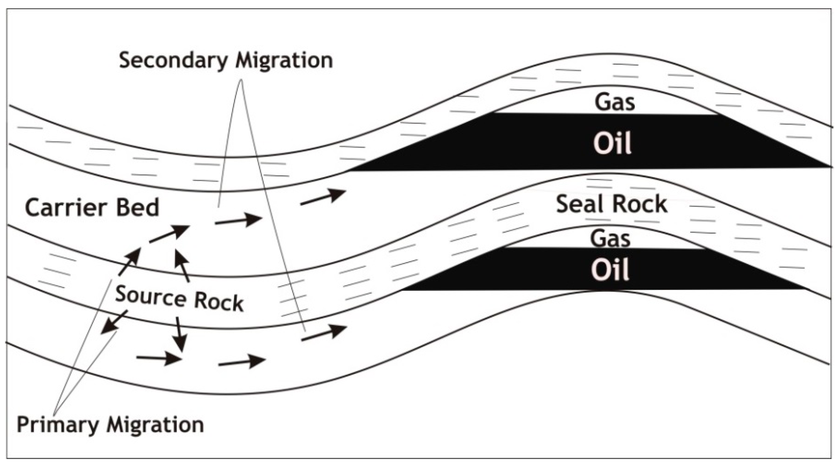
:1. Introduction
2. Formulation of the Problem and Study Methodology
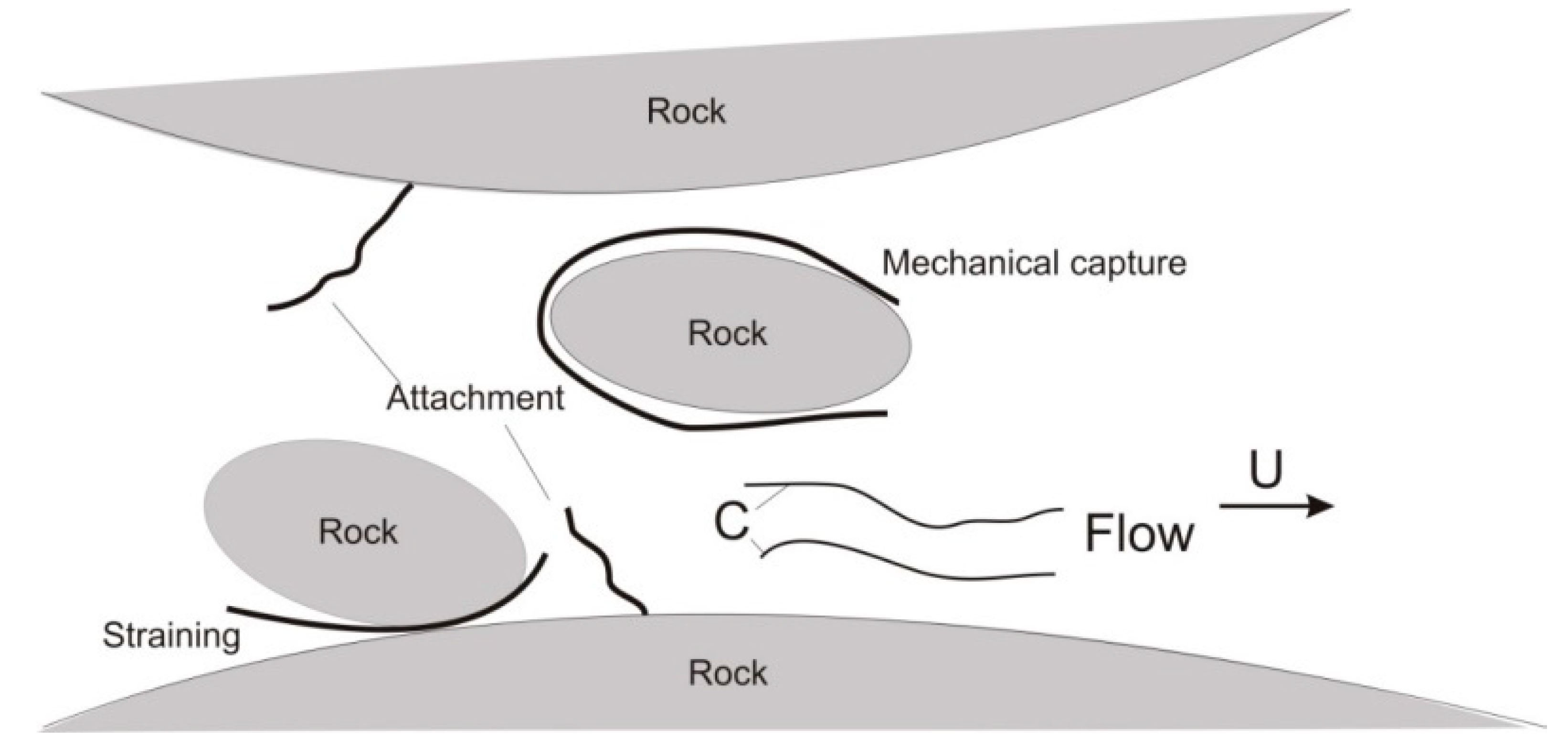
3. Deep Bed Filtration of Colloidal Suspensions in Porous Media
4. Mathematical Model for Secondary Migration with Particle Retention
4.1. Assumptions of the Model
4.2. Analytical Model for Steady-State Flow of Components
4.3. Determination of Filtration Coefficient Versus X
5. Numerical Results
6. Effects of Stress on Compositional Gradients of Migrating Oil
Example
7. Discussions
8. Conclusions
- An analytical model for deep bed filtration of petroleum components facilitates matching the component concentrations in source rock and reservoir.
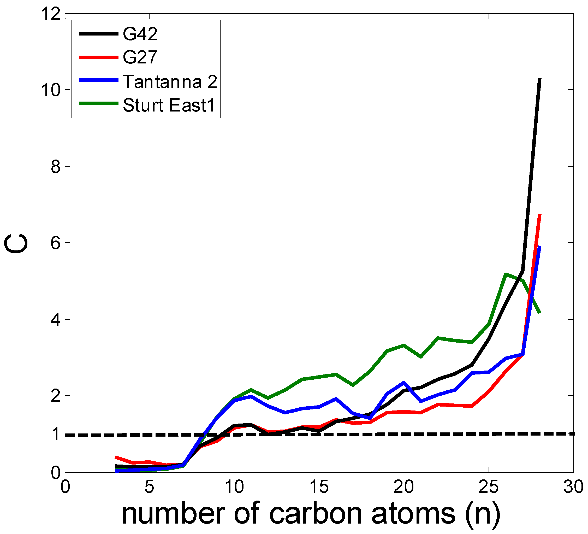
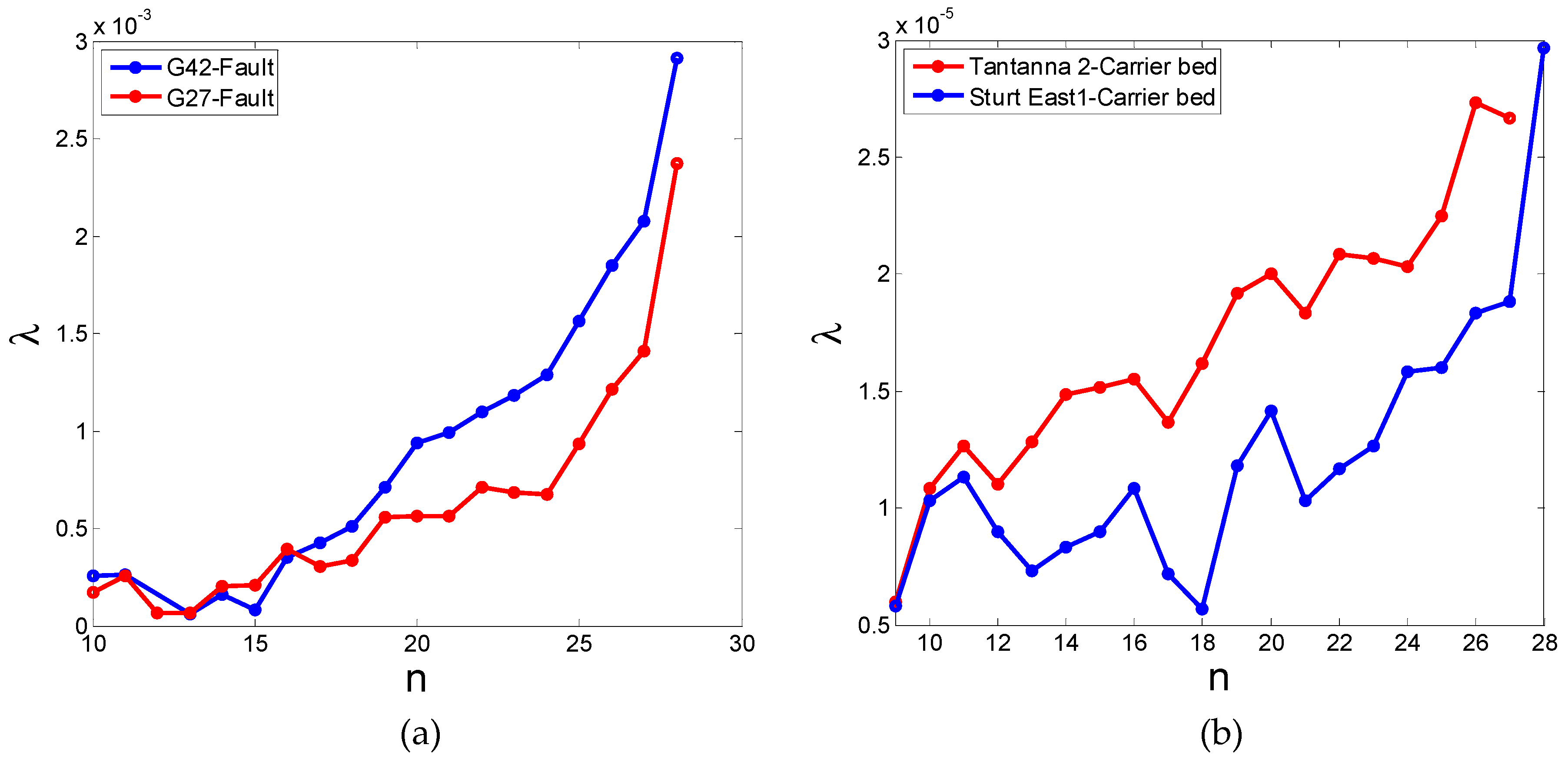
- For heavy hydrocarbons with n>10, the obtained values of filtration coefficients vary in the typical intervals. The heavier the component, the larger the filtration coefficient.
- For light and intermediate hydrocarbons with n<10, the tendency of monotonicity does not take place, which is explained by evaporation into associated gas phase that migrates together with oil.
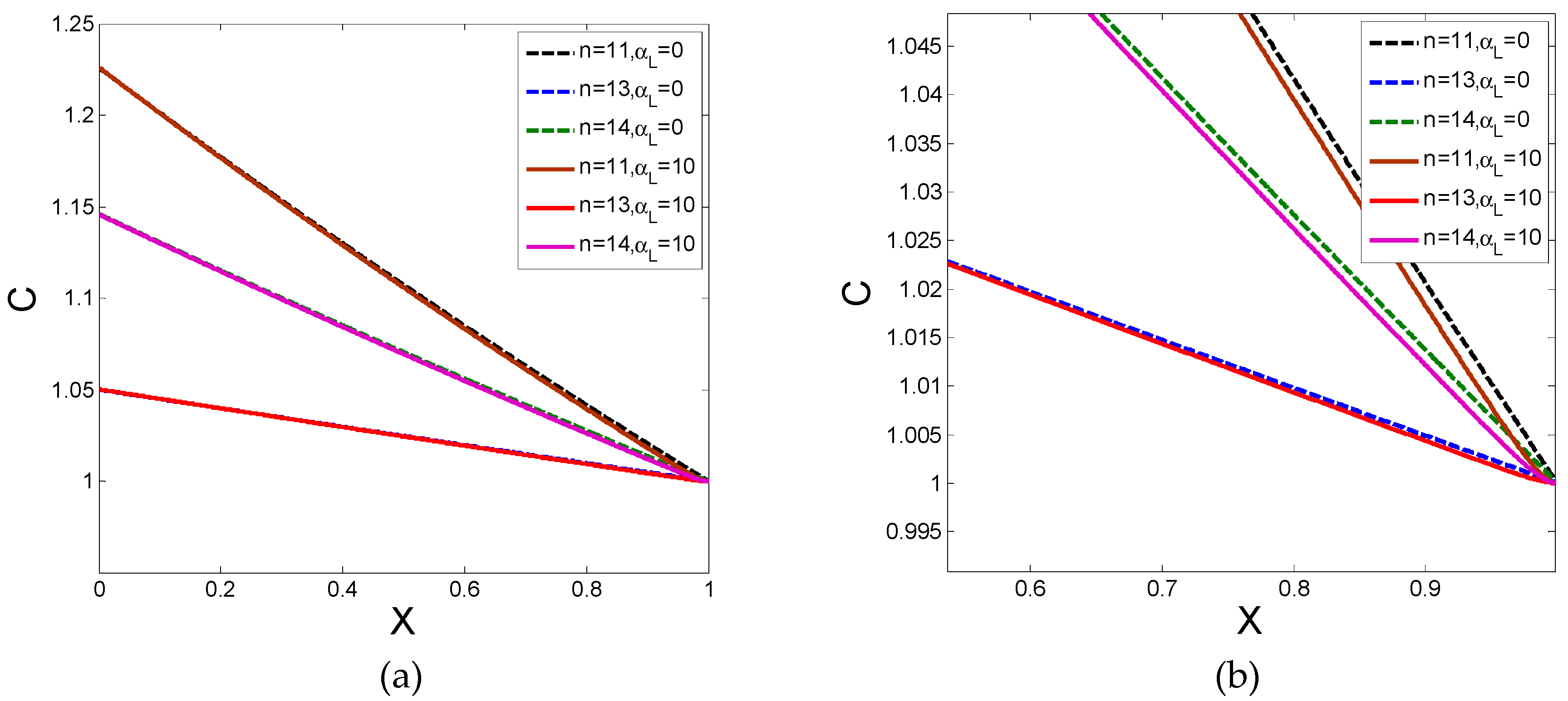
- Comparison between modelling with and without the component dispersion shows a negligible effect of dispersion on compositional difference between the source rock and petroleum reservoir.
- Higher stress yields to the lower porosity and lower permeability, which results in a smaller pore size and higher deep bed coefficients.
Author Contributions
Funding
Conflicts of Interest
References
- England, W.A.; Mann, A.L.; Mann, D.M. Migration from Source to Trap: Chapter 3: Petroleum Generation and Migration; BP Research: London, UK, 1991. [Google Scholar]
- Magoon, L.B.; Dow, W.G. The petroleum system-from source to trap. AAPG Mem. 1994, 60, 1–24. [Google Scholar]
- Siddiqui, F.I.; Lake, L.W. A dynamic theory of hydrocarbon migration. Math. Geol. 1992, 24, 305–327. [Google Scholar] [CrossRef]
- Helset, H.M.; Lake, L.W. Three-phase secondary migration of hydrocarbon. Math. Geol. 1998, 30, 637–660. [Google Scholar] [CrossRef]
- Bessis, B.; Burrus, F.; Ungerer, J.P.; Chenet, P.Y. Integrated Numerical Simulation of the Sedimentation Heat Transfer, Hydrocarbon Formation and Fluid Migration in a Sedimentarybasin, the THEMIS Model. In Thermal Modelling in Sedimentary Basins; Burrus, J., Ed.; Technip: Paris, France, 1986; pp. 173–195. [Google Scholar]
- Galushkin, Y. Non-Standard Problems in Basin Modelling. Springer International Publishing: Basel, Switzerland, 2016. [Google Scholar]
- Baur, F.; Scheirer, A.H.; Peters, K. Past, present and the future of basin and petroleum system modeling. AAPG Bull. 2017, 102, 549–561. [Google Scholar] [CrossRef]
- Peters, K.E.; Schenk, O.; Scheirer, A.H.; Wygrala, B.; Hantschel, T. Basin and Petroleum System Modeling. In Springer Handbook of Petroleum Technology 2017; Springer: Cham, Switzerland, 2017; pp. 381–417. [Google Scholar]
- Baur, F.; Katz, B. Some practical guidance for petroleum migration modelling. Mar. Pet. Geol. 2018, 93, 409–421. [Google Scholar] [CrossRef]
- Lake, L.W. Enhanced Oil Recovery; Prentice Hall: Englewood Clis, NJ, USA, 1989. [Google Scholar]
- Bedrikovetsky, P.G. Mathematical Theory of Oil & Gas Recovery; Kluwer Academic Publishers: London, UK; Boston, MA, USA; Dordrecht, The Netherlands, 1993. [Google Scholar]
- Carruthers, D. Modeling of Secondary Petroleum Migration Using Invasion Percolation Techniques. In AAPG/Datapages Discovery Series: Multidimensional Basin Modeling; Duppenbecker, S., Marzi, R., Eds.; AAPG/Datapages: Tulsa, OK, USA, 2003; pp. 21–37. [Google Scholar]
- Carruthers, D.; Ringrose, P. Secondary oil migration: Oil-rock contact volumes, flow behaviour and rates. Geol. Soc. Lond. Spec. Publ. 1998, 144, 205–220. [Google Scholar] [CrossRef]
- Carruthers, D.J.; de Lind van Wijngaarden, M. Modelling viscous-dominated fluid transport using modified invasion percolation techniques. J. Geochem. Explor. 2000, 69–70, 669–672. [Google Scholar] [CrossRef]
- Dejam, M.; Hassanzadeh, H.; Chen, Z. A reduced-order model for chemical species transport in a tube with a constant wall concentration. Can. J. Chem. Eng. 2018, 96, 307–316. [Google Scholar] [CrossRef]
- Dejam, M.; Hassanzadeh, H.; Chen, Z. Shear dispersion in a capillary tube with a porous wall. J. Contam. Hydrol. 2016, 185–186, 87–104. [Google Scholar] [CrossRef]
- Dejam, M.; Hassanzadeh, H.; Chen, Z. Shear dispersion in a fracture with porous walls. Adv. Water Resour. 2014, 74, 14–25. [Google Scholar] [CrossRef]
- Sun, Z.; Shi, J.; Wu, K.; Xu, B.; Zhang, T.; Chang, Y.; Li, X. Transport capacity of gas confined in nanoporous ultra-tight gas reservoirs with real gas effect and water storage mechanisms coupling. Int. J. Heat Mass Transf. 2018, 126, 1007–1018. [Google Scholar] [CrossRef]
- Riemens, W.G.; Schulte, A.M.; De Jong, L.N.J. Bibra Field PVT variations along the hydrocarbon column and confirmatory field Test. J. Petrol. Tech. 1988, 40, 83–89. [Google Scholar] [CrossRef]
- Wheaton, R.J. Treatment of variations of composition with depth in gas-condensate reservoirs. SPE Reserv. Eng. 1991, 6, 239–244. [Google Scholar] [CrossRef]
- Shapiro, A.A.; Stenby, E.H. Two-Phase Segregation in a Thick Reservoir. In Proceedings of the ECMOR V-5th European Conference on the Mathematics of Oil Recovery, Leoben, Austria, 3–6 September 1996. [Google Scholar]
- Montel, F.; Bickert, J.; Lagisquet, A.; Galliéro, G. Initial state of petroleum reservoirs: A comprehensive approach. J. Pet. Sci. Eng. 2007, 58, 391–402. [Google Scholar] [CrossRef]
- Faissat, B.; Knudsen, K.; Stenby, E.H.; Montel, E. Fundamental statements about thermal diffusion for a multicomponent mixture in a porous medium. Fluid Ph. Equilib. 1994, 100, 209–222. [Google Scholar] [CrossRef]
- Kulikowski, D.; Amrouch, K. Combining geophysical data and calcite twin stress inversion to refine the tectonic history of subsurface and offshore provinces: A case study on the Cooper-Eromanga Basin, Australia. Tectonics 2017, 36, 515–541. [Google Scholar] [CrossRef]
- Firoozabadi, A. Thermodynamics of Hydrocarbon Reservoirs; McGraw-Hill: New York, NY, USA, 1999; 353p. [Google Scholar]
- Whitson, C.H.; Brulé, M.R. Phase Behavior; Henry, L., Ed.; Doherty Memorial Fund of AIME Society of Petroleum Engineers: Richardson, TX, USA, 2000. [Google Scholar]
- Nikpoor, M.H.; Dejam, M.; Chen, Z.; Clarke, M. Chemical-gravity-thermal diffusion equilibrium in two-phase non-isothermal petroleum reservoirs. Energy Fuels 2016, 30, 2021–2034. [Google Scholar] [CrossRef]
- Shapiro, A.A.; Stenby, E.H. On the nonequilibrium segregation state of a two-phase mixture in a porous column. Transp. Porous Media 1996, 23, 83–106. [Google Scholar] [CrossRef]
- Heath, R.; McIntyre, S.; Gibbins, N. A Permian Origin for Jurassic Reservoired Oil in the Eromanga Basin. In The Cooper and Eromanga Basins, Australia; O’Neil, B.J., PESA, SPE, SEG, Eds.; Petroleum Society of Australia: Adelaide, Australia, 1989; pp. 405–415. [Google Scholar]
- Lowe-Young, B.S.; Mackie, S.L.; Heath, R.S. The Cooper-Eromanga petroleum system, Australia: Investigation of essential elements and processes. In Proceedings of the Petroleum Systems of SE Asia and Australasia Conference, Jakarta, Indonesia, 21–23 May 1997; pp. 199–211. [Google Scholar]
- Farajzadeh, R.; Bedrikovetsky, P.; Lotfallahi, M.; Lake, L. Simultaneous sorption and mechanical entrapment during polymer flow through porous media. J. Water Resour. Res. 2016, 52, 2279–2298. [Google Scholar] [CrossRef] [Green Version]
- Barenblatt, G.I.; Entov, V.M.; Ryzhyk, V.M. Theory of Fluid Flows Through Natural Rocks; Kluwer Academic Publishers: Dordrecht, The Netherlands, 1990. [Google Scholar]
- Pope, G.A. The application of fractional flow theory to enhanced oil recovery. SPE J. 1980, 20, 191–205. [Google Scholar] [CrossRef]
- Sorbie, K.S. Polymer-Improved Oil Recovery; Springer Science and Business Media: Berlin, Germany, 2013. [Google Scholar]
- Lotfollahi, M.; Farajzadeh, R.; Delshad, M.; Al-Abri, A.-K.; Wassing, B.M.; Al-Mjeni, R.; Awan, K.; Bedrikovetsky, P. Mechanistic Simulation of Polymer Injectivity in Field Tests. SPE J. 2016, 21, 1–14. [Google Scholar] [CrossRef]
- Bedrikovetsky, P. Upscaling of stochastic micro model for suspension transport in porous media. J. Transp. Porous Media 2008, 75, 335–369. [Google Scholar] [CrossRef]
- Herzig, J.P.; Leclerc, D.M.; Le Goff, P. Flow of suspensions through porous media—Application to deep filtration. J. Ind. Eng. Chem. 1970, 65, 8–35. [Google Scholar] [CrossRef]
- Bedrikovetsky, P.; You, Z.; Badalyan, A.; Osipov, Y.; Kuzmina, L. Analytical model for straining-dominant large-retention depth filtration. Chem. Eng. J. 2017, 330, 1148–1159. [Google Scholar] [CrossRef]
- Bradford, S.A.; Simunek, J.; Bettahar, M.; Van Genuchten, M.T.; Yates, S.R. Modeling colloid attachment, straining, and exclusion in saturated porous media. Environ. Sci. Technol. 2003, 37, 2242–2250. [Google Scholar] [CrossRef] [PubMed]
- Bradford, S.A.; Torkzaban, S. Colloid Transport and Retention in Unsaturated Porous Media: A Review of Interface-, Collector-, and Pore-Scale Processes and Models. Vadose Zone J. 2008, 7, 667–681. [Google Scholar] [CrossRef]
- Elimelech, M. Particle deposition onideal collectors from dilute flowing suspensions: Mathematical formulation, numerical solution, and simulations. J. Sep. Technol. 1994, 4, 186–212. [Google Scholar] [CrossRef]
- Elimelech, M.; Gregory, J.; Jia, X. Particle Deposition and Aggregation; Butterworth-Heinemann: Oxford, UK, 1995. [Google Scholar]
- Pang, S.; Sharma, M.M. A Model for Predicting Injectivity Decline in Water-Injection Wells. SPE J. 1997, 12, 194–201. [Google Scholar]
- Wennberg, K.E.; Sharma, M.M. Paper SPE 38181: Determination of the Filtration Coefficient and the Transition Time for Water Injection Wells. In Proceedings of the SPE European Formation Damage Conference, The Hague, The Netherlands, 2–3 June 1997. [Google Scholar]
- Santos Ltd. Gidgealpa 27 Well Completion Report; PPL 6 Moomba Block; Cooper & Eromanga Basins; Santos Ltd.: Adelaide, Australia, 1988. [Google Scholar]
- Santos Ltd. Sturt East 1 Well Completion Report; PEL 5 and 6 Lake Hope Block; Cooper & Eromanga Basins; Santos Ltd.: Adelaide, Australia, 1989. [Google Scholar]
- Santos Ltd. Tantanna 2 Well Completion Report; PEL 5 & 6 Lake Hope Block; Eromanga Basin; Santos Ltd.: Adelaide, Australia, 1989. [Google Scholar]
- Santos Ltd. Gidgealpa 42 Well Completion Report; PPL 6 Moomba Block; Cooper & Eromanga Basins; Santos Ltd.: Adelaide, Australia, 1991. [Google Scholar]
- Kulikowski, D.; Amrouch, K.; Cooke, D.; Gray, M.E. Basement structural architecture and hydrocarbon conduit potential of polygonal faults in the Cooper-Eromanga Basin, Australia. Geophys. Prospect. 2017. [Google Scholar] [CrossRef]
- Deighton, I.; Hill, A.J. Thermal and burial history. In Petroleum Geology of South Australia; Gravestock, D.I., Hibburt, J., Drexel, J.F., Eds.; Petroleum Group: Adelaide, Australia, 1998; Volume 4, pp. 143–155. [Google Scholar]
- Person, M.; Raffensperger, J.P.; Garven, G. Basin-scale hydrogeological modelling. Rev. Geophys. 1996, 34, 61–87. [Google Scholar] [CrossRef]
- Logan, D.J. Transport Modeling in Hydrogeochemical Systems; Springer: New York, NY, USA, 2001. [Google Scholar]
- Polyanin, A.; Zaitsev, V. Handbook of Nonlinear Partial Differential Equations; Chapman and Hall/CRC Press: Boca Raton, FL, USA, 2011. [Google Scholar]
- Israelachvili, J. Intermolecular and Surface Forces; Academic Press: Millbrae, CA, USA, 2006. [Google Scholar]
- Nicolaevskij, V.N. Mechanics of Fractured and Porous Media. In World Scientific Series Theoretical and Applied Mechanics; World Scientific: Singapore; Hackensack, NJ, USA; London, UK, 1990; Volume 8. [Google Scholar]
- Dake, L.P. The Practice of Reservoir Engineering; Elsevier: Amsterdam, The Netherlands, 2013; Volume 36. [Google Scholar]


| Carbon Number n | λ × 103 1/m, without Diffusion, for Well G42 | λ × 103 1/m, with Diffusion, for Well G42, αL = 10 m | λ × 103 1/m, without Diffusion, for Well G27 | λ × 103 1/m, with Diffusion, for Well G27, αL = 10 m | λ × 104 1/m, without Diffusion, for Well T2 | λ × 104 with Diffusion for Well T2 αL = 100 | λ × 104 1/m, without Diffusion, for SE1 | λ × 104 with Diffusion for Well SE1 αL = 100 |
|---|---|---|---|---|---|---|---|---|
| 2 | 0.314 | 0.319 | 0.25 | 0.25 | ||||
| 9 | 0.06 | 0.06 | 0.058 | 0.058 | ||||
| 10 | 0.255 | 0.265 | 0.173 | 0.176 | 0.108 | 0.108 | 0.103 | 0.103 |
| 11 | 0.261 | 0.259 | 0.259 | 0.2635 | 0.127 | 0.127 | 0.113 | 0.113 |
| 12 | 0.066 | 0.067 | 0.11 | 0.11 | 0.09 | 0.09 | ||
| 13 | 0.0615 | 0.0617 | 0.0853 | 0.0866 | 0.128 | 0.128 | 0.073 | 0.073 |
| 14 | 0.170 | 0.173 | 0.2024 | 0.205 | 0.148 | 0.148 | 0.083 | 0.083 |
| 15 | 0.083 | 0.082 | 0.206 | 0.209 | 0.152 | 0.152 | 0.09 | 0.09 |
| 16 | 0.3541 | 0.358 | 0.393 | 0.400 | 0.155 | 0.155 | 0.108 | 0.108 |
| 17 | 0.429 | 0.434 | 0.304 | 0.309 | 0.137 | 0.137 | 0.072 | 0.072 |
| 18 | 0.5215 | 0.529 | 0.337 | 0.342 | 0.162 | 0.162 | 0.056 | 0.056 |
| 19 | 0.715 | 0.726 | 0.558 | 0.567 | 0.192 | 0.192 | 0.118 | 0.118 |
| 20 | 0.941 | 0.961 | 0.568 | 0.576 | 0.2 | 0.2 | 0.142 | 0.142 |
| 21 | 0.994 | 1.01 | 0.558 | 0.567 | 0.183 | 0.183 | 0.103 | 0.103 |
| 22 | 1.11 | 1.13 | 0.712 | 0.721 | 0.208 | 0.208 | 0.117 | 0.117 |
| 23 | 1.18 | 1.21 | 0.690 | 0.7 | 0.207 | 0.207 | 0.126 | 0.126 |
| 24 | 1.288 | 1.32 | 0.68 | 0.69 | 0.203 | 0.203 | 0.158 | 0.158 |
| 25 | 1.56 | 1.60 | 0.931 | 0.956 | 0.225 | 0.225 | 0.16 | 0.16 |
| 26 | 1.85 | 1.90 | 1.22 | 1.241 | 0.273 | 0.273 | 0.183 | 0.183 |
| 27 | 2.07 | 2.15 | 1.41 | 1.45 | 0.267 | 0.267 | 0.188 | 0.188 |
| 28 | 2.91 | 3.04 | 2.38 | 2.46 | 0.233 | 0.233 | 0.296 | 0.296 |
© 2019 by the authors. Licensee MDPI, Basel, Switzerland. This article is an open access article distributed under the terms and conditions of the Creative Commons Attribution (CC BY) license (http://creativecommons.org/licenses/by/4.0/).
Share and Cite
Borazjani, S.; Kulikowski, D.; Amrouch, K.; Bedrikovetsky, P. Composition Changes of Hydrocarbons during Secondary Petroleum Migration (Case Study in Cooper Basin, Australia). Geosciences 2019, 9, 78. https://doi.org/10.3390/geosciences9020078
Borazjani S, Kulikowski D, Amrouch K, Bedrikovetsky P. Composition Changes of Hydrocarbons during Secondary Petroleum Migration (Case Study in Cooper Basin, Australia). Geosciences. 2019; 9(2):78. https://doi.org/10.3390/geosciences9020078
Chicago/Turabian StyleBorazjani, Sara, David Kulikowski, Khalid Amrouch, and Pavel Bedrikovetsky. 2019. "Composition Changes of Hydrocarbons during Secondary Petroleum Migration (Case Study in Cooper Basin, Australia)" Geosciences 9, no. 2: 78. https://doi.org/10.3390/geosciences9020078