The Hyper-Angular Cube Concept for Improving the Spatial and Acoustic Resolution of MBES Backscatter Angular Response Analysis


1
Institute for Mediterranean Studies, Foundation of Research and Technology—Hellas, Melissinou & Nikiforou Foka 130, P.O. Box. 119, Rethymno 74100, Greece
2
GEOMAR Helmholtz Center for Ocean Research, Kiel 24148, Germany
3
Christian-Albrechts University Kiel, Institute of Geosciences; Ludewig-Meyn-Str. 10-12, 24098 Kiel, Germany
*
Author to whom correspondence should be addressed.
Geosciences 2018, 8(12), 446; https://doi.org/10.3390/geosciences8120446
Submission received: 16 October 2018
/
Revised: 24 November 2018
/
Accepted: 27 November 2018
/
Published: 30 November 2018
(This article belongs to the Special Issue Geological Seafloor Mapping)
Abstract
:This study presents a novel approach, based on high-dimensionality hydro-acoustic data, for improving the performance of angular response analysis (ARA) on multibeam backscatter data in terms of acoustic class separation and spatial resolution. This approach is based on the hyper-angular cube (HAC) data structure which offers the possibility to extract one angular response from each cell of the cube. The HAC consists of a finite number of backscatter layers, each representing backscatter values corresponding to single-incidence angle ensonifications. The construction of the HAC layers can be achieved either by interpolating dense soundings from highly overlapping multibeam echo-sounder (MBES) surveys (interpolated HAC, iHAC) or by producing several backscatter mosaics, each being normalized at a different incidence angle (synthetic HAC, sHAC). The latter approach can be applied to multibeam data with standard overlap, thus minimizing the cost for data acquisition. The sHAC is as efficient as the iHAC produced by actual soundings, providing distinct angular responses for each seafloor type. The HAC data structure increases acoustic class separability between different acoustic features. Moreover, the results of angular response analysis are applied on a fine spatial scale (cell dimensions) offering more detailed acoustic maps of the seafloor. Considering that angular information is expressed through high-dimensional backscatter layers, we further applied three machine learning algorithms (random forest, support vector machine, and artificial neural network) and one pattern recognition method (sum of absolute differences) for supervised classification of the HAC, using a limited amount of ground truth data (one sample per seafloor type). Results from supervised classification were compared with results from an unsupervised method for inter-comparison of the supervised algorithms. It was found that all algorithms (regarding both the iHAC and the sHAC) produced very similar results with good agreement (>0.5 kappa) with the unsupervised classification. Only the artificial neural network required the total amount of ground truth data for producing comparable results with the remaining algorithms.
1. Introduction
Seafloor acoustic mapping with multibeam echosounders (MBES) faces the emergence of new data acquisition styles, which also trigger the development of new data processing and interpretation approaches. Acquiring MBES datasets using multiple frequencies [1] or acquiring backscatter-dedicated MBES surveys [2,3] enormously increased the volume of data per seafloor area, leading to increased dimensionality of MBES datasets. At the same time, novel data processing methods appeared for improving the accuracy and detail of geo-information about the seafloor. Although sparse in number, there are studies that paved the way for more advanced seafloor mapping. In particular, those techniques which incorporate the angular dependence of the seafloor backscatter are considered more robust and preferable for seafloor classification. This is due to the fact that the angular dependence is a physical property of the seafloor backscatter which was validated both by model and in situ data [4,5].
Combination of angular response analysis (ARA) with modern remote-sensing methods such as object-based image analysis (OBIA) and machine learning algorithms are considered state-of-the-art in the field of seafloor mapping. Recent studies incorporated these techniques and produced some promising results. For instance, Reference [6] applied various supervised classification techniques integrating backscatter measurements from 71 incidence angles for benthic habitat mapping. Furthermore, Reference [7] utilized the random forest algorithm in conjunction with ARA features (such as skewness and kurtosis of angular curves) and bathymetric features for benthic habitat mapping, while Reference [8] employed ARA and pattern recognition methods for classifying sediment types. Both studies [7,8] applied OBIA for backscatter mosaic segmentation. Similarly, Reference [9] combined bathymetric features and angular response curves using a neural network model for mapping seafloor sediments.
In most cases, two major issues arise in traditional ARA of MBES backscatter data. These issues are related to the spatial resolution of ARA results and the separability of angular responses. The issue of spatial resolution occurs because angular responses are usually extracted from coarse seafloor patches with the size of half of the MBES swath. In addition, the separability of backscatter responses has an impact on discrimination of various seafloor types. Another problem considered in the studies of References [3,6] is the performance of traditional supervised classifiers using a restricted amount of ground truth data along with high-dimensional spatial datasets. The first two issues are highlighted by References [5,10,11]. They propose that ARA should be based on backscatter measurements from homogeneous seafloor areas in order to better discriminate their angular responses. In addition, References [8,9] raise the necessity for calculating an n-dimensional backscatter matrix (n is the number of backscatter mosaics corresponding to n number of incidence angle ensonifications) using the measurements from each incidence angle, for extracting angular responses per cell and, thus, increasing class separation and the spatial resolution of the classification map.
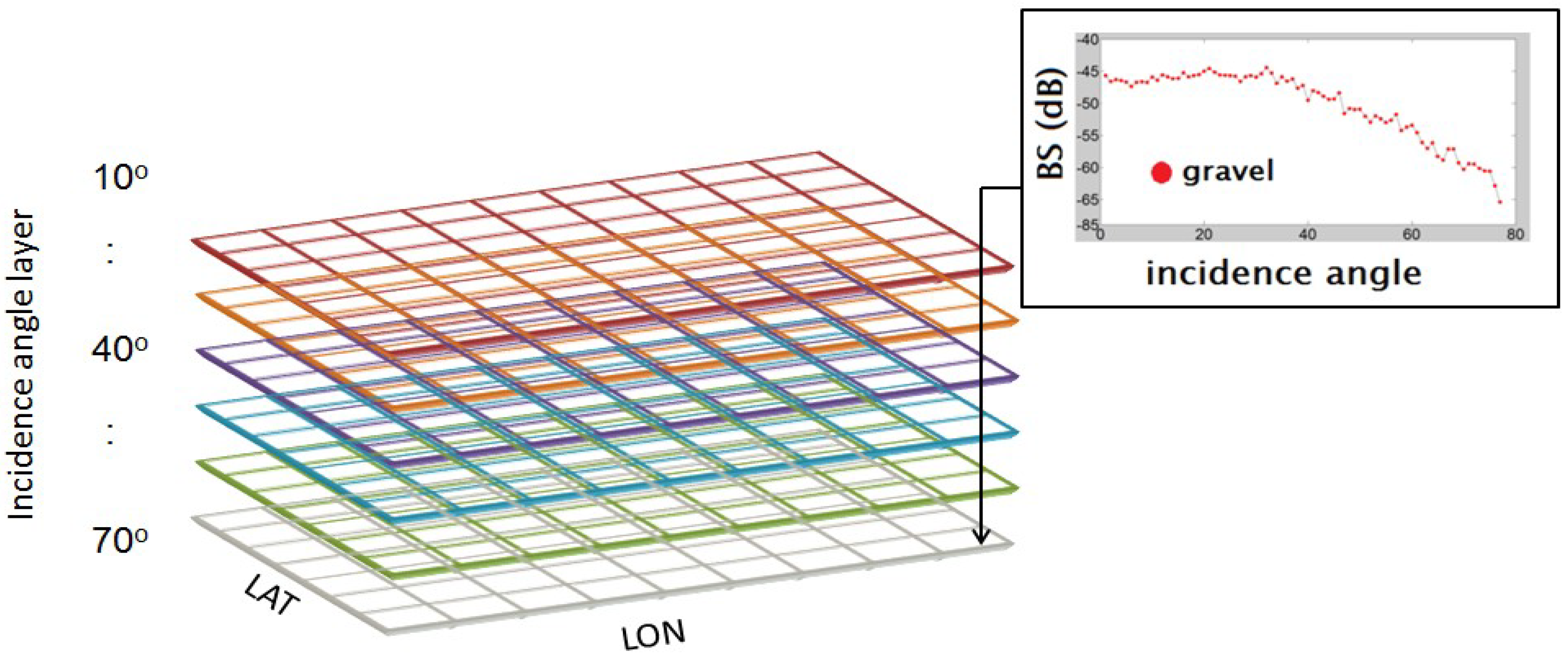
The idea of such a matrix was presented firstly by Reference [10] and initially implemented by Reference [11] using only sparse soundings. According to their concept, the cells of a matrix should be densely populated with backscatter values from multiple incidence angles (yielded by MBES surveys with high degree of overlap >100%) which result in dense soundings per seafloor area. Despite the practical limitations of such surveys, the advantages of the resulting datasets are significant regarding discrimination of acoustic classes. Additionally, the resulting classification maps can be constructed with a spatial resolution comparable to that of ground truth data and the MBES footprint (meter scale), a fact that increases their validity and usefulness for the end-users [12]. Since the implementation of Reference [11], the above concept of an n-dimensional backscatter matrix was only later employed again, in the studies of References [3,13], where they took advantage of the high density of MBES soundings resulting from a backscatter-dedicated survey with >100% overlap. Interpolation of backscatter values from individual incidence angles was used for producing angular backscatter layers which were then stacked together to form the so-called hyper-angular cube matrix (HAC), which is presented here (Figure 1). Similarly, References [14,15] produced a number of backscatter mosaics, each representing measurements according to a reference incidence angle, for applying predictive mapping of the seafloor along with other descriptive variables.
Study Objectives
Considering that extracting angular responses from the lowest level of acoustic elements (i.e., the grid cells of a backscatter layer/mosaic) is the way forward in improving the performance of ARA, and that the HAC provides this possibility in a solid way, we focused the scope of this paper on utilizing an HAC from MBES data with high overlap and, alternatively, from MBES data with standard overlap. We present a method to construct the HAC from MBES data with standard overlap in order to overcome the practical limitations of backscatter-dedicated surveys, thus minimizing the time and cost of the fieldwork. This method was recently considered in the literature by References [14,15]. In addition, we examined and compared the performance of four supervised machine learning classifiers in terms of class separation and how to deal with a restricted amount of training data along with the high-dimensional HAC dataset. Building a high-resolution HAC from MBES data of standard overlap and exploiting a small amount of ground-truth samples for classification will have an impact on future backscatter studies by decreasing the cost of data collection, while, at the same time, maximizing the usability and quality of acoustic and ground-truth datasets.
2. Materials and Methods
2.1. The Hyper-Angular Cube Matrix
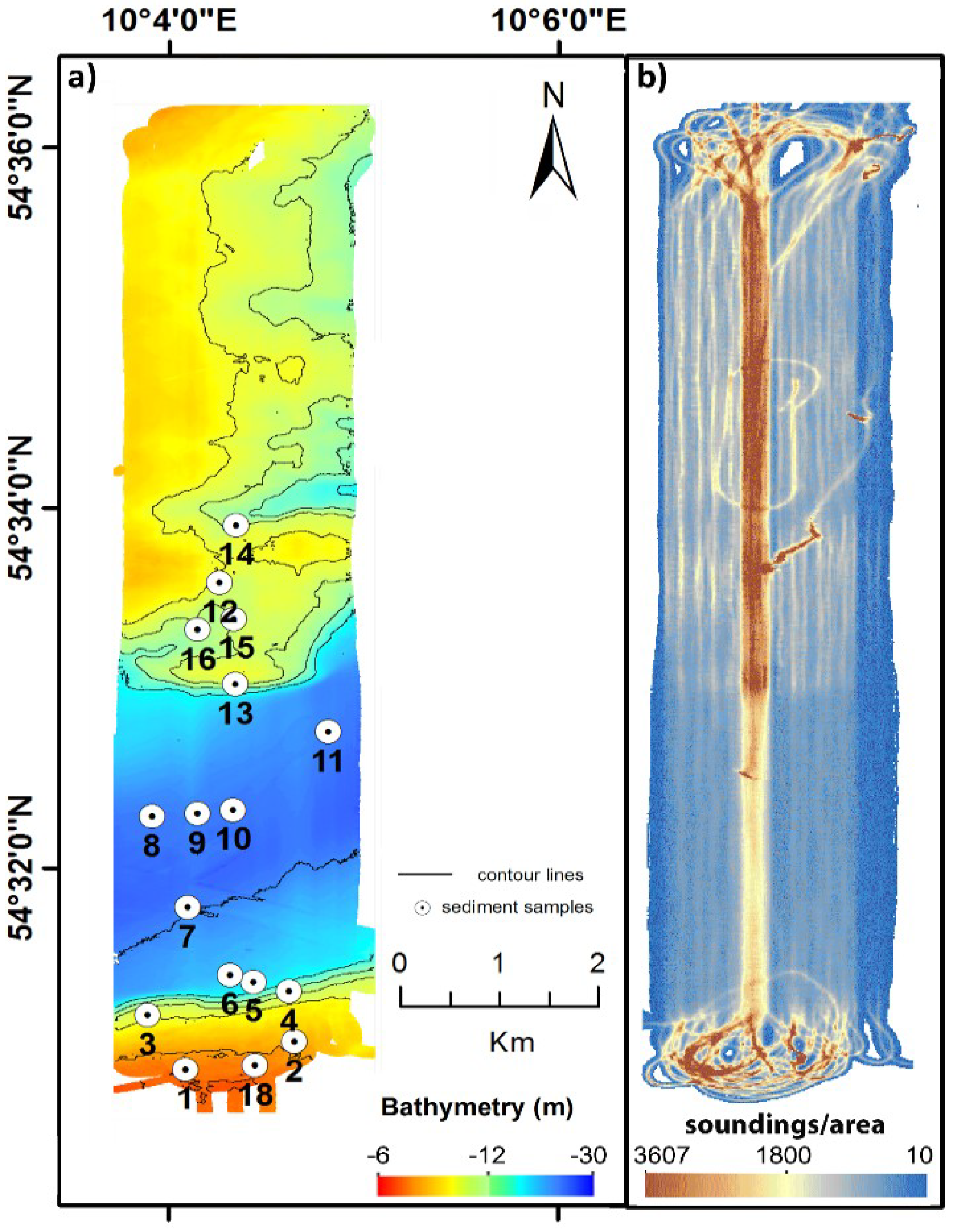
The hydro-acoustic dataset was obtained in 2012 using an ELAC Nautik (ELAC Nautik, Kiel, Germany) 1180 MBES sonar at 180 kHz. The survey track lines had varying spacing from 15 to 40 m, resulting in dense ensonifications per seafloor area spanning a narrow corridor of north–south orientation that holds 6 to 30 m of water depth (Figure 2). Accordingly, we produced 23 interpolated backscatter layers for separate incidence angles in the range of 10° to 65° in steps of 2° in the middle-range beams and 3° for the beams close to nadir and outer range. Interpolation for each of the 23 backscatter layers was performed using the inverse distance-weighted (IDW) algorithm with 10-m search radius and an output cell size of 5 m. Stacking of all layers defined a hyper-angular cube structure (interpolated HAC, iHAC) for which an angular signature per cell could be extracted (Figure 1).
This approach requires dense soundings per seafloor area. However, since collection of such data increases the ship time and total cost of the MBES survey, it is not always the most suitable option to follow. Alternatively, we examined a method for obtaining an HAC matrix efficiently and without the costs of a backscatter-dedicated survey (i.e., with >100% overlap). Our approach was based on producing backscatter mosaics (using MBES data with standard overlap), each being normalized with different reference angle values. Usually, a backscatter mosaic is produced by normalizing the backscatter intensities falling within a sliding window according to the value of middle-range incidence angles (e.g., 30°, 40°, or 40–60° average). Using the middle-range incidence angles as reference for normalizing the backscatter values (removing the angular dependence) is a standard practice which was supported by the study of Reference [16]. They suggested that the backscatter intensity from the 45° incidence angle can be used as a useful proxy for correlations with geological features, and that it has the potential for discriminating more seafloor types than the backscatter from the near- and far-range incidence angles. The studies of References [16,17,18] converge to the following explanation about why 45° is widely accepted in sediment mapping. According to their studies, backscatter measurements from incidence angles near the nadir are more susceptible to the specular effect that results in similar (high) dB values for different seafloor types, making them indiscernible. Furthermore, backscatter measurements from the outer range are affected by reflection of the backscatter energy to all directions due to the very low grazing angle, resulting in similar (low) dB values for any seafloor type. As a result, incidence angles from the middle range yield backscatter measurements with sufficient contrast that allows for seafloor characterization. Thus, in most software packages for backscatter processing, there is no option for selecting the reference angle for angle normalization. However, the MB System (utilized in this study) and the CMST-GA MB Process [11,18] are two known software packages that allow choosing the reference angle (and sliding window size) for backscatter mosaicking. MB System was applied here for producing 23 backscatter mosaics (using selected MBES lines with less than 100% overlap), each being normalized at a different reference angle (same as the number of iHAC layers). By stacking these mosaics, we obtained a synthetic version of the HAC (sHAC) from which we could extract a full angular response from each individual cell.
It has to be noted that, for obtaining useful angular responses, the MBES sonar should record backscatter intensity in a stable and linear way [19]. Ideally, the original data should be geometrically (seafloor slope, footprint area) and radiometrically (beam pattern, time-varying gain (TVG)) corrected, such that the data represent changes only depending on the seafloor type variations [18,20,21]. In this study, we extracted the raw backscatter values from the sonar files using the HDPPost software by ELAC Nautik; then, we created, for each incidence angle, a file with X,Y and corresponding backscatter value, which was then used for building the iHAC. It was not necessary to apply seafloor slope corrections to the data as the study area has a very smooth bathymetry (<<5° for the majority of slopes). For constructing the sHAC, we applied the corrections that are included in the MB System software for the particular type of MBES. Following the corrections to the backscatter measurements, the generation of angle-normalized mosaics takes place. Normalizing a backscatter mosaic at a certain (reference) incidence angle is an important step for building the sHAC, since each mosaic should reflect seafloor changes as if it was ensonified only by one particular incidence angle. Angle normalization is an empirical method for removing the angular dependence from the backscatter data, applied by References [17,20,22,23]. There are several variations of this method that were applied in literature, and, in this study, we used the one implemented in the MB System software. This approach is based on the method in References [17,23] that subtracts the mean backscatter value calculated for all incidence angles over a user-defined sliding window of several consecutive pings (30 pings in this study). The mean backscatter value of the reference incidence angle is then added to the residual values of each individual ping in order to adjust their values to the level of the reference incidence angle (Equation (1)). Equation (1) gives an example for angle normalization using the reference values for the 40° incidence angle. This approach is considered better than other empirical approaches [18] and it outputs mosaics where specific seafloor types are highlighted more than others depending on the incidence angle used for normalization. This is a crucial feature for analyzing seafloor types using the sHAC.
where is the backscatter value of an individual incidence angle, is the average backscatter value over several pings and is the backscatter value of the 40° incidence angle (reference angle).
After correcting and normalizing the backscatter data, it is possible to apply some image enhancement techniques to further improve the quality of the mosaics. Mosaic enhancements, such as despeckle or feathering, for example, should be applied in cases that the data are affected by noise. Another way of improving mosaic quality is to exclude data from the nadir area (e.g., incidence angles of 0–5°) and outer range (e.g., incidence angles of >70°). In our study, we excluded data from incidence angles lower than 10° and greater than 65°; however, there was no need to apply any special image-enhancement technique.
2.2. Supervised Machine Learning Algorithms
Soundings from within matrix cells corresponding to ground-truth locations shown in Table 1 were utilized as training data in the following supervised classifiers: a pattern recognition approach (sum of absolute differences, SAD), random forest (RF), support vector machine (SVM), and an artificial neural network (ANN). Each algorithm was applied on both types of HAC matrices, i.e., that made of interpolated backscatter layers (iHAC) and that made from angle-normalized mosaics (sHAC). These algorithms were selected since traditional supervised classification with the maximum likelihood classification (MLC) method has some limitations regarding the quality and quantity of training samples and the dimensionality of the backscatter data [24].
In supervised classification, the training data provide the “knowledge” regarding each defined class that assist the algorithm in classifying the rest of the (unknown) data. The “knowledge” consists of a set of input data including the angular responses of each incidence angle and the corresponding seafloor type value (categorical). In this study, we use the term “descriptors” to refer to the angular layers of the iHAC or the sHAC from which the angular responses were obtained.
The pattern recognition approach used here (SAD) is described in Reference [13], where it was initially implemented. The method compares the two-dimensional (2D) shape of known angular signatures with unknown ones. A similarity assessment is used for comparison of both signatures which are treated as 2D vectors. The level of similarity with each of the reference signatures determines the acoustic class membership of the unknown angular signatures. An adaptation of the SAD algorithm for 2D data was used for testing the similarity of angular signatures.
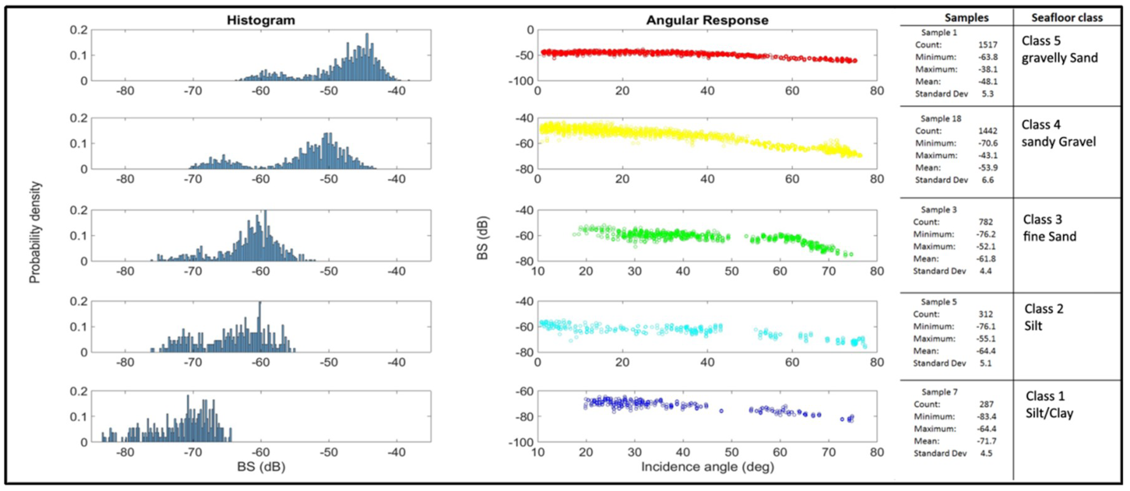
The SAD algorithm was initially developed for video compression and it is widely used for object recognition tasks [25]. In our implementation, the algorithm calculated the difference between reference and unknown backscatter values of corresponding incidence angles. Then, similarity criteria were applied to the sum of differences for each class assignment. It is implied that the lower the values of the sum of absolute differences are, the higher is the similarity between the 2D objects (angular signatures) under examination will be. The user has to set only two criteria that will influence the similarity assessment and, hence, the final classification results. These criteria include the standard deviation offset and the majority criterion. The standard deviation offset criterion controls the maximum acceptable absolute differences between known and unknown angular signatures. It is obtained by means of data exploration of soundings falling within the ground-truth cells (Figure 3).
Soundings forming the angular signature of known seafloor types hold particular standard deviations for each seafloor type (Figure 3). This information helps in defining tolerance boundaries for the mean backscatter values of each seafloor type. The standard deviation offset can be used for strict or fuzzy class membership. The majority criterion controls the number of incidence angles, the difference values of which fall within the acceptable standard deviation offset. Accordingly, the majority criterion needs always to be set as large as possible (>80%) for more robust matching. It should be adjusted only if backscatter information is missing for certain angles. This algorithm was implemented in Matlab code and it is described in Reference [13].
The RF is a machine learning algorithm that is widely applied in image analysis and predictive seafloor mapping studies [26,27]. The training process is based on “growing” several (user-defined) classification trees using random subsets of the training sample as a priori information. This information is then compiled into a non-parametric model for classifying the grid cells of the input layers. The prediction at a certain grid cell is defined by the majority votes of all random subsets of trees [28]. Growing of classification trees is iterative; thus, each time (during the training), the RF reserves randomly selected parts of the training sample (out-of-bag sample) for internal cross-validation of the results. With each iteration, one descriptor value is neglected and its importance score is calculated according to its contribution to the resulting prediction error. Descriptor importance is considered one of the main advantages of the RF algorithm. The RF approach was initially applied together with ARA by References [6,7] and on angle-normalized mosaics by References [29,30]. The studies of References [6,7] used angular responses extracted from half swath measurements within objects (groups of cells) derived by automated segmentation of the backscatter mosaic. In this study, we applied the RF on the grid cells of layers building up the HAC matrices described above. The algorithm can identify non-linear relationships that underlie backscatter values and the seafloor types. In addition, it outputs a rating with the importance scores for each angular layer indicating their influence in predicting a certain seafloor type. For this application, the Marine Geospatial Ecology Toolbox (MGET) software [31] (http://mgel2011-kvm.env.duke.edu/mget) was used.
The SVM is a machine learning algorithm which is particularly used for supervised classification of terrestrial multispectral data and, recently, for seafloor acoustic mapping [6,32]. In a study by Reference [6], they applied the SVM on backscatter mosaic objects, whereas, in this study, we applied the algorithm on cells of the HAC layers. The SVM maximizes the separation of classes in a high-dimensional dataset by fitting a hyper-dimensional plane (or just hyperplane) to the data feature space. The hyperplane is produced using a kernel function when the data cannot be linearly separated in feature space. The selection of a particular type of kernel function depends on the data separation pattern (in feature space) and will have a strong effect on classification. The SVM has the ability to identify non-linear relationships within the data, and does not require normal distribution of the training backscatter values from within each acoustic class. The SVM used in this study was implemented in the OpenCV library provided by the System for Automated Geoscientific Analyses (SAGA).
Finally, an ANN approach was examined in this study. ANNs mimic the functionality of biological neurons and they are extensively used in speech/face recognition, and also in landscape classification studies [33,34]. They possess a number of advantages that distinguish them from common algorithms, whereas they also hold some disadvantages. Regarding the merits of ANNs, these include not making any assumptions about the data (e.g., a normal distribution of training data is not a prerequisite for data analysis), being able to identify non-linear relationships in high-dimensional data, and, most importantly, acquiring learning without the input of physical models that describe data variability. However, ANNs are considered as black boxes regarding input–output of data, and they require several trial-and-error iterations for optimal tuning of algorithm settings. In this study, two training sets were used to support the ANN classification. The main concept of a supervised ANN is that an input of variables is examined in a combinatorial way regarding the production of certain outputs. The combination of variables leading to acceptable outputs (according to the training set) is determined by weight factors that strengthen the relationship between the input and output. Learning occurs when the ANN modifies the weight factors via a back-propagation technique in order to minimize a user-defined error rate value. The trained ANN then applies its “knowledge” to the rest of the dataset for classification of unknown elements. The ANN was applied to backscatter angular responses initially by Reference [9], producing promising results. However, they used seafloor patches generated from a half-swath sliding window to extract the angular responses. This fact had an effect on the homogeneity of the angular responses and hindered class separability in their study. The ANN used in this study was implemented in the OpenCV library provided by SAGA.
2.3. Training Set Selection
In this study we tested all classifiers using a training set with fixed size, meaning that angular responses from only five representative ground-truth locations were utilized (Figure 4c, Table 1 and Figure 3). The sediment samples of Table 1 were collected using a multi-corer and a Van-Veen grab. The selection of the training set was based on grain size analysis results and information from an unsupervised classification [3]. The unsupervised method applied in [3] yielded an optimum number of five classes therefore it was considered as guiding information for the supervised training in this study. The small amount of training set was chosen to fit the purpose of the study in assessing the ability of machine learning classifiers to perform adequate classification using a restricted amount of training set. Only the ANN method required the total number of ground-truth data during training for producing results comparable to the rest of the classifiers.
3. Results
3.1. Comparison of Angular Responses from Dense Soundings with Interpolated and Synthetic Cubes (iHAC and sHAC)
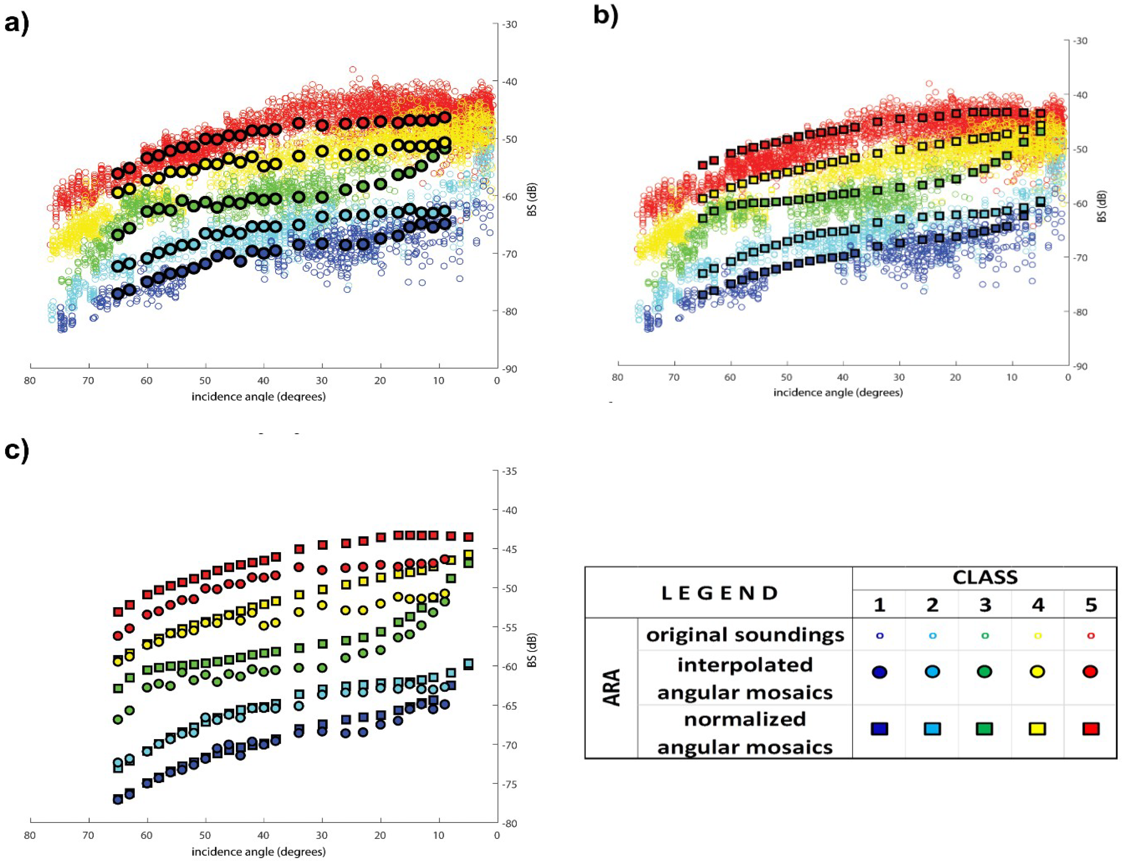
In this study, we extracted the angular responses of five different seafloor types in three different ways. Firstly, we extracted the original soundings from within 5 × 5 m2 rectangular patches corresponding to the five ground-truth locations (Figure 2a, Table 1). These resulted in multiple backscatter values for all incidence angles and each seafloor type being represented by a distinct cloud of measurements. In addition, we extracted angular responses from the cells of the two matrices (iHAC and sHAC) corresponding to the five ground-truth locations. In the first instance, the iHAC consisted of a set of 23 backscatter layers resulting from interpolation of original dense backscatter measurements. In the second instance, the sHAC consisted of backscatter mosaics resulting from angle normalization using 23 reference incidence angles each time. It was observed that all three sets of extracted angular responses clearly distinguished the five seafloor types individually and separately from each other (Figure 4). Each angular response followed a hierarchical plan from coarser to finer material, meaning that angular responses of coarse seafloor types held higher decibel (dB) values than those of the fine types in all instances. It appears that the angular responses derived from the cells of iHAC correspond close to the mean dB values of the original angular response cloud. The angular responses derived from the cells of the sHAC appear smoother than those derived from the iHAC and with positive offset between 1 to 3 dB. In general, angular responses derived from both the iHAC and sHAC were suitable for seafloor classification using ARA since they hold continuous and distinctive information for each of the five seafloor types. Considering the suitability of the above angular responses for seafloor mapping, we applied the supervised classifiers on iHAC and sHAC data for classifying the seafloor of the study area. The classification maps resulting from the iHAC angular mosaics are shown in Figure 5.
3.1.1. SAD
The SAD algorithm uses a set of reference angular signatures representing a known seafloor type (class) (Figure 4c) for comparison with unknown signatures extracted from each grid cell of the HAC. Matching is based on criteria set by the user (standard deviation offset, majority) and each cell is assigned with the class represented by the successfully matched reference signature. In this study, the offset value was selected according to the standard deviation of dB values from each angular signature; thus, different offsets were applied for each class (Figure 3). The majority threshold was set to 90% of the total number of incidence angles. Some cells could be matched with up to two adjacent angular signatures and receive double class assignment. In this regard, class overlap was quantified and it was found to affect class boundaries of neighboring classes (Figure 5). Cells without continuous angular signatures or cells that did not conform to the majority criterion remained unclassified.
3.1.2. RF
The training sample for RF consists of several hundreds of angular backscatter values derived from five ground-truth locations (Figure 4a,b, Table 1). We fitted models using 50, 100, 200, 500, and 1000 trees and found that all of them produced a zero out-of-bag error rate (OOB). This is an indication that the training sample is particularly effective and produces consistently correct results regardless of the number of trees used to fit the model. Additionally, it was found that, regarding variable importance, some differences occurred when fitting was done using a low (50) and high (500) number of trees. When the model was fitted with 50 trees, almost half of the angular layers scored much higher importance values for predicting all classes. On the other hand, when 500 trees were used for model fitting, the importance scores were much lower for the majority of angular layers regarding prediction of all classes. The individual class importance scores varied for each class and for the number of trees as well. In general, for the model fitted with 50 trees, the importance scores varied individually for each class, while angular layers of 50° and 60° incidence consistently received the lowest scores (zeroes). When a model with a relatively higher number of trees (500) was applied, the importance scores tended to differentiate more clearly two groups of classes, i.e., the prediction of classes 1 and 2 was influenced more by a few angular layers from the near range (11°, 13°, 15°, and 17°), a few angular layers from the middle range (40°, 44°, and 48°), and a few angular layers from the outer range (54°, 63°, and 65°). In contrast, prediction of classes 3 to 5 was found to be equally influenced by all angular layers.
3.1.3. SVM
Polygons corresponding to the grid cells of five reference ground-truth locations were used as training areas. The SVM requires a user-defined kernel function for fitting a hyperplane to separate the acoustic classes. In this study, we tested a number of kernel functions and it was found that linear, polynomial (C0 = 1, deg = 0.5, gamma = 1) and histogram-intersection functions provided the most convincing classification results (Figure 5). In contrast, radial basis, sigmoid, and exponential-x2 kernel functions produced poor to non-realistic classification results. The effectiveness of the above kernel functions was related to the separation pattern of angular backscatter values in feature space. Therefore, a suitable kernel function is one that fits better the class boundaries in the hyper-dimensional feature space.
3.1.4. ANN
We ran ANN using (a) the polygons holding the five reference ground-truth locations, and (b) all polygons holding ground-truth information (18 locations) (Figure 2a, Table 1). The classification results showed a more realistic appearance when the total ground-truth data were used for training. One single layer was chosen for model simplicity and a Gaussian function (alpha = 1, beta = 1) was applied as an activation function that adjusted the weight factors of model outputs during the learning process. An activation function is fundamental for ANN learning and its selection is not related to the features of the training set. The Gaussian function was chosen because it was the only one to produce reasonable classification results comparable to the results of the three classifiers applied. The number of neurons was set to 18, the same as the number of training areas [9].
3.2. Validation
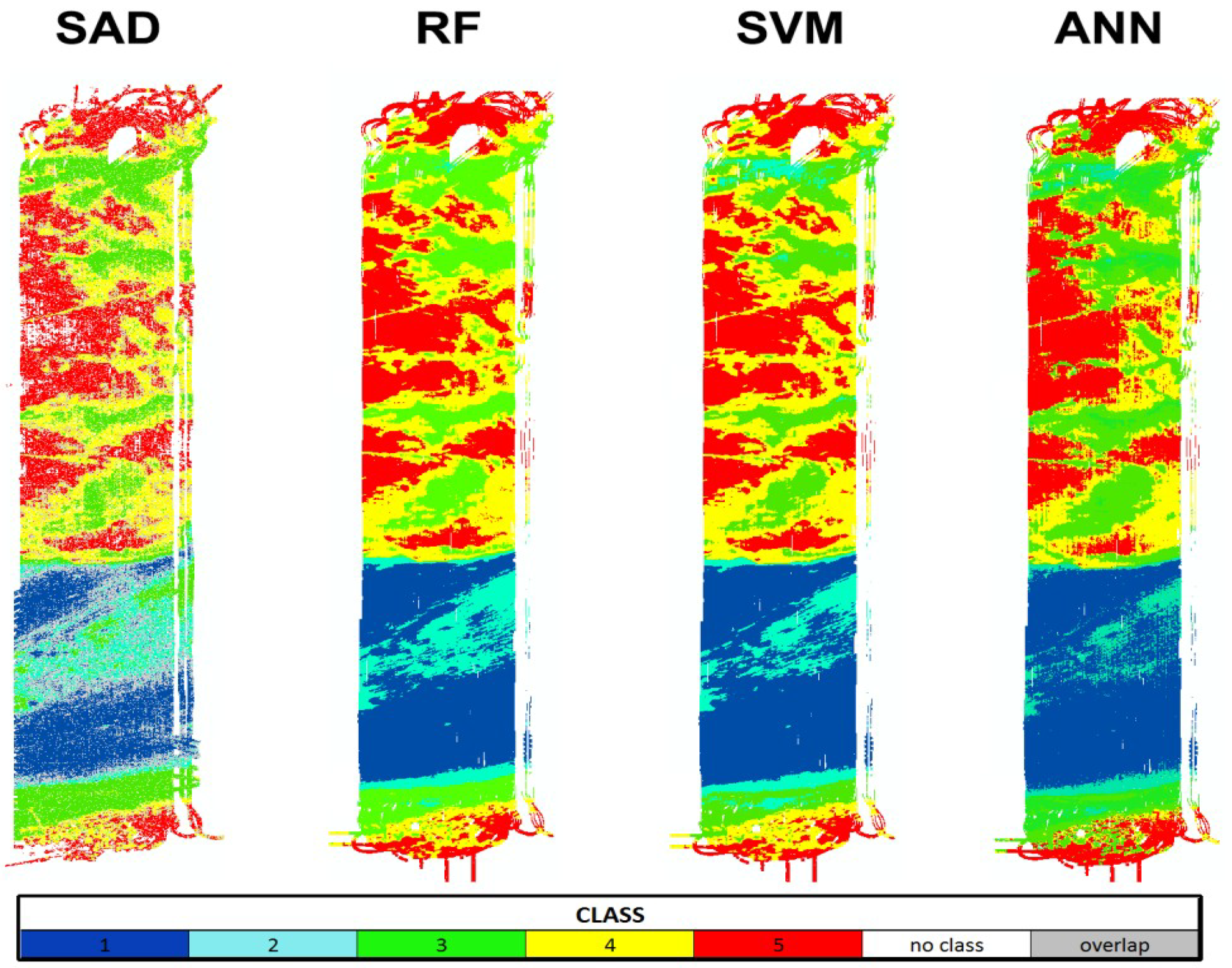
All classifiers produced very similar classification results (Figure 5, Table 2) and, thus, showed great potential in automated supervised seafloor classification using high-dimensional MBES backscatter datasets with a limited amount of ground-truth data for training. Only the ANN classifier required a greater amount of training data (threefold) for producing classification results comparable to the other classifiers. The final classification maps expressed an agreement in the areal percentage per class, and it could also be seen that all classes covered comparable geographical areas among each of the maps. Table 2 shows results of each supervised classification map when compared to the classification map of Reference [3]. This map is considered to represent sediment variability in a more objective way, since it was produced by an unsupervised method that performs cluster validation. The comparison was done with the Map Comparison Kit implemented in Reference [35] (http://mck.riks.nl) and agreement was quantified using kappa, kappa histogram (K Hist), and kappa location (K Loc) coefficients. The kappa coefficient is a standard measure of agreement between two categorical maps, while the kappa histogram expresses the agreement regarding the amount of cells belonging to each class, and the kappa location expresses the agreement of class assignment by location (i.e., high kappa location score means that all areas were classified similarly between the two maps). All scores suggested strong agreement between each classification map and the Bayesian classification map of Reference [3] with minor fluctuations. The scores of the classification maps produced using the sHAC appeared slightly lower than the scores of the classification maps produced using the interpolated HAC, but this difference is not statistically significant (i.e., both iHAC and sHAC scores in Table 2 belong to the highest ranking of agreement). This difference occurred because the backscatter mosaics of the sHAC contained some noise in the nadir and outer ranges, which was not possible to remove from the data, leading to misclassification of a small number of cells.
4. Discussion
4.1. Effectiveness of the HAC Matrix for Improving the Spatial and Acoustic Resolution of ARA
Until now, the main approach to overcome the problem of acoustic class homogeneity in ARA studies was by segmenting the backscatter mosaic into objects (groups of cells) using algorithms requiring several user-defined parameters. Then, angular responses were extracted from soundings falling within each object, assuming that they better discriminate the corresponding seafloor types. The concept examined in this study takes ARA one step forward by introducing the HAC matrix.
The HAC matrix approach presented here allows for extraction of angular signatures from the lowest level of spatial constituents (i.e., the grid cells of the HAC layers), eliminating the need for backscatter mosaic segmentation. Angular signatures derived from fine-scale homogeneous seafloor areas (grid cells similar to the average MBES footprint size) are relevant to the scale of ground-truth data, supporting the highest possible separation of seafloor types. In this way, along swath seafloor variations can be resolved and acoustic classes can be assigned for each grid cell and not coarse seafloor patches. These two facts are expected to advance seafloor mapping by offering more detailed acoustic classification results that are consistent with seafloor acoustic properties (i.e., angular dependence of backscatter). Highly detailed seafloor classification maps can effectively depict fine-scale variations of sediments on the seafloor and provide valuable input to benthic habitat and other studies that rely on effective separation of seafloor sediments.
The layers building the HAC matrix may result either from interpolation of spatially dense backscatter values of each incidence angle (iHAC) or by producing normalized backscatter mosaics using different incidence angles for reference each time (sHAC). The iHAC requires backscatter-dedicated MBES surveys with more than 100% overlap for obtaining dense soundings per seafloor area. Since backscatter-dedicated MBES surveys are time-consuming (thus, costly), the sHAC is a useful alternative. The shape of angular responses yielded from the iHAC may appear less smooth than those derived from the sHAC. This occurs because the cell values of the iHAC reflect the effects of the natural seafloor variability from actual soundings values, while the sHAC cell values represent angular variability based on calculation of average local backscatter intensity. Thus, it is essential to select an appropriate number of pings for averaging during the angle-normalization process. Averaging over a relatively large number of pings (i.e., including backscatter values from many seafloor types) will produce an sHAC, the angular signatures of which might be very smooth and possibly overlapping/non-distinguishable. It is suggested that the optimal number of pings may be estimated using the pings within a certain radius from the ground-truth locations. Pings from within a small radius should form well-shaped angular signatures which gradually (with increasing radius) produce more mixed signatures.
Although the dB values of our data are not absolute (MBES not calibrated), they comply with the standards of Reference [19] for repetitive seafloor mapping, meaning that they are stable (repeatable over the same type of seafloor) and linear (changing according to changes in seafloor type in the same way). This fact allows for suggesting a theoretical framework, according to which our empirically derived angular responses can be compared to those derived by the Applied Physics Laboratory (APL) model [4]. Initially, it was observed that the empirical angular responses (Figure 4c) obey the rule of angular dependence of seafloor backscatter. This means that, for responses resulting from rough seafloor with coarse sediment grain sizes, there is not a large dB difference between the incidence angles close to nadir and the middle part of the swath. Accordingly, responses resulting from a smooth seafloor with fine sediment grain sizes show a more pronounced difference in dB values between the nadir area and the middle part of the swath (due to the specular effect). Similarly, there is a clear decrease of the dB values for the outer swath incidence angles for all seafloor types. This behavior is in agreement with the pattern observed in the theoretical angular response curves produced by the APL model. Moreover, both the APL curves and HAC responses show a decreasing offset (of dB values) for sediments with decreasing grain sizes (Figure 4). Considering that both the APL and HAC angular responses show similar geometrical characteristics, it can be suggested that the HAC responses rely on a geophysical base, and, by applying a suitable transformation (e.g., simple offset or a linear transformation), this may assist in calibrating the output dB values of the HAC layers. Calibrating the HAC layers according to absolute dB values will offer the possibility of applying geophysical models (such as the APL) for inferring seafloor properties per cell. Such a development is going to offer the possibility for the HAC concept to be adopted by software developers in an effort to improve the traditional ARA approach. However, it has to be noted that geophysical models such as the APL provide only a limited range of angular curves, thus covering only the most common sediment types, since these models are based mainly on experimental data; thus, it is not practical to examine the full range of seafloor types in the laboratory. In reality, the seafloor includes numerous combinations of the most common sediment types along with a great variety of substrates (e.g., corals, macroalgae). The advantage of the empirically derived angular responses is that they are representative of the seafloor heterogeneity from which they are derived from. In addition, a comprehensive set of angular responses can be produced for each seafloor type identified from ground-truth information. This can occur only when the shape of the angular responses is sufficiently different between similar seafloor types, and when the MBES outputs stable and linear dB measurements. Concluding, it is suggested that future MBES backscatter software may incorporate the utility of the sHAC allowing the user to produce a stack of angle-normalized mosaics and to identify particular seafloor types on cells of these mosaics based on ground-truth data locations. In this way, the user can construct a set of empirically derived angular responses that will then be applied for classifying the entire dataset.
The HAC concept is an objective way of deriving homogeneous angular responses in contrast to applying backscatter mosaic segmentation. Mosaic segmentation requires expert knowledge which can be subjective, and, by varying the segmentation parameters, different angular responses may be obtained. Considering the results of this study, we suggest that future backscatter studies should either rely on dense backscatter soundings (for using the iHAC) or on MBES surveys with conventional overlap, but producing several backscatter mosaics normalized for different incidence angles each time, to generate the sHAC. In addition, a small amount of highly overlapping lines may/should be collected over known seafloor for validation purposes.
4.2. Suitability of Machine Learning Algorithms for Advanced Seafloor Mapping Using the HAC
Testing the performance of the four applied machine learning classifiers (SAD, RF, SVM, and ANN) revealed valuable information about new capabilities for automated MBES backscatter classification. A particular aspect in this study is the application of these algorithms on the HAC matrix. This type of data structure allows for exploiting the angular dependence of backscatter within a new processing concept, while preserving the high spatial resolution of angular backscatter layers. One important finding is that the majority of the above classifiers produce valid classification results using only a small but representative amount of ground-truth training data. Thus, careful selection of ground-truth information is crucial for the performance of machine learning classifiers. It is suggested that each seafloor type should be represented by at least one training area. This implies that even the minimum amount of ground-truth data (one sample per seafloor type) is enough for classification, as long as the data come from acoustically and geologically distinct areas.
As a result, careful planning of ground-truth sampling prior to classification should take place, and it should consider variations in backscatter data as well. In the case that the training set consists of polygon cells (e.g., for SVM and ANN), the cell size should be set at the same size as the grid cell size of the HAC layers. This affects the quality of angular responses considered and will have an impact on the class separation when the sediment variability is high within a few meters. It is implied that very large cell sizes will result in more mixed angular signatures and may produce inconsistent classification results. The same holds for the case when the training data are points (e.g., for SAD and RF). Angular responses of reference seafloor types should be continuous and sufficiently separated from each other.
Backscatter values that are encompassed by either training areas or points are not required to have normal distribution when the described classifiers are used. Performing accurate seafloor classification using high-dimensional acoustic data, even with a small training set, is a very common situation in the field of seafloor mapping. The above algorithms in conjunction with the HAC structure will decrease the time and cost for ground-truth data collection, by effectively using a smaller but representative amount of seafloor samples.
5. Conclusions
In this study, the concept of the HAC matrix was considered for improving the application of ARA using multiple angular backscatter layers with minimal ground-truth information. There are two ways of constructing the HAC layers, one of which is based on interpolation of actual soundings (iHAC) from single incidence angles (i.e., from backscatter-dedicated surveys with large overlap). The other is to produce backscatter mosaics using a different normalization angle each time (sHAC). Both HAC types yield comparable angular responses per cell, which is the finest element of the matrix layers. This guarantees that angular responses come from naturally homogenous areas of the seafloor, thus providing trustworthy comparisons with the ground-truth data and eliminating the need for backscatter mosaic segmentation.
The sHAC provides the possibility of collecting MBES data with standard overlap and obtaining angular responses per cell as efficiently as with using an iHAC. Thus, the sHAC minimizes the costs of backscatter-dedicated surveys and seems as a promising alternative in ARA classification. The high dimensionality of the HAC matrices makes them ideal inputs to machine learning algorithms for advanced supervised seafloor classification by incorporating the angular backscatter information. Machine learning algorithms require the input of ground-truth data for training. Practical limitations are usually responsible for collecting small amounts of ground-truth data, and this presents another challenge in seafloor mapping. In this study, we tested the performance of four machine learning algorithms using the HAC layers and only one sample per seafloor type for classification. All four algorithms produced very comparable results that were in agreement with the classification results from an unsupervised method used as reference. The HAC approach described here shows potential in future ARA studies by maximizing acoustic class homogeneity and providing improved class separability. The use of machine learning algorithms in conjunction with high-dimensional angular backscatter layers provides a reliable tool for fast, automated seafloor classification that integrates angular backscatter information in an effective way.
Author Contributions
Conceptualization, E.A.; methodology, E.A.; software, E.A.; validation, E.A. and J.G.; formal analysis, E.A.; investigation, E.A.; resources, J.G.; data curation, J.G.; writing—original draft preparation, E.A.; writing—review and editing, E.A. and J.G.; supervision, J.G.; project administration, E.A.
Funding
This research received no external funding.
Acknowledgments
We would like to specifically thank Sebastian Krastel (Institute of Geosciences, Christian-Albrechts-Universität, Kiel) and Christian Berndt (GEOMAR) for providing access to the MBES dataset that they collected in 2012. We would also like to thank captain and crew of RV Littorina, for their support throughout the ground truth data survey. This is publication 39 of the DeepSea Monitoring group at GEOMAR. Publication of this manuscript received financial support from the funding program Open Access Publikationsfonds provided by the federal state of Schleswig-Holstein (Germany).
Conflicts of Interest
The authors declare no conflict of interest.
References
- Hughes-Clarke, J.E. Multispectral Acoustic Backscatter from Multibeam—Improved Classification Potential, U.S. In Proceedings of the Hydrographic Conference, National Harbor, MD, USA, 16–19 March 2015. [Google Scholar]
- Augustin, J.-M.; Lamarche, G. High redundancy multibeam echosounder backscatter coverage over strong relief. In Seabed and Sediment Acoustics: Measurements and Modelling Conference; University of Bath: Bath, UK, 2015; p. 37. [Google Scholar]
- Alevizos, E.; Snellen, M.; Simons, D.G.; Siemes, K.; Greinert, J. Multi-angle backscatter classification and sub-bottom profiling for improved seafloor characterization, Special Issue “Seafloor backscatter from swath echosounders: technology and applications”. Mar. Geophys. Res. 2017, 39, 289–306. [Google Scholar] [CrossRef]
- APL-UW. High-Frequency Ocean Environmental Acoustic Models Handbook (APL-UW TR 9407); Applied Physics Laboratory, University of Washington: Seattle, WA, USA, 1994. [Google Scholar]
- Fonseca, L.; Brown, C.; Calder, B.; Mayer, L.; Rzhanov, Y. Angular range analysis of acoustic themes from Stanton Banks Ireland: A link between visual interpretation and multibeam echosounder angular signatures. Appl. Acoust. 2009, 70, 1298–1304. [Google Scholar] [CrossRef]
- Hasan, R.C.; Ierodiaconou, D.; Laurenson, L. Combining angular response classification and backscatter imagery segmentation for benthic biological habitat mapping. Estuar. Coast. Shelf Sci. 2012, 97, 1–9. [Google Scholar] [CrossRef] [Green Version]
- Che Hasan, R.; Ierodiaconou, D.; Laurenson, L.; Schimel, A. Integrating multibeam backscatter angular response; mosaic and bathymetry data for benthic habitat mapping. PLoS ONE 2014, 9, e97339. [Google Scholar] [CrossRef] [PubMed]
- Rzhanov, Y.; Fonseca, L.; Mayer, L. Construction of seafloor thematic maps from multibeam acoustic backscatter angular response data. Comput. Geosci. 2012, 41, 181–187. [Google Scholar] [CrossRef]
- Huang, Z.; Siwabessy, J.; Nichol, S.; Anderson, T.; Brooke, B. Predictive mapping of seabed cover types using angular response curves of multibeam backscatter data: Testing different feature analysis techniques. Cont. Shelf Res. 2013, 61–62, 12–22. [Google Scholar] [CrossRef]
- Clarke, J.H. Towards remote seafloor classification using the angular response of acoustic backscattering: A case study from multiple overlapping GLORIA data. IEEE J. Oceanic Eng. 1994, 19, 112–127. [Google Scholar] [CrossRef]
- Parnum, I.M. Benthic habitat mapping using multibeam sonar systems. Ph.D. Thesis, Curtin University, Perth, Australian, 2007. [Google Scholar]
- McGonigle, C.; Brown, C.; Quinn, R.; Grabowski, J. Evaluation of image-based multibeam sonar backscatter classification for benthic habitat discrimination and mapping at Stanton Banks UK. Estuar. Coast. Shelf Sci. 2009, 81, 423–437. [Google Scholar] [CrossRef]
- Alevizos, E. An object-based seafloor classification tool using recognition of empirical angular backscatter signatures. In Proceedings of the GEOHAB 2017, Halifax, Canada, 1–5 May 2017. [Google Scholar] [CrossRef]
- Huang, Z.; Siwabessy, J.; Nichol, S.L.; Brooke, B.P. Predictive mapping of seabed substrata using high-resolution multibeam sonar data: a case study from a shelf with complex geomorphology. Mar. Geol. 2014, 357, 37–52. [Google Scholar]
- Huang, Z.; Siwabessy, J.; Cheng, H.; Nichol, S. Using multibeam backscatter data to investigate sediment-acoustic relationships. J. Geophys. Res. Ocean. 2018, 123, 4649–4665. [Google Scholar] [CrossRef]
- Lamarche, G.; Lurton, X.; Verdier, A.-L.; Augustin, J.-M. Quantitative characterisation of seafloor substrate and bedforms using advanced processing of multibeam backscatter-Application to Cook Strait; New Zealand. Cont. Shelf Res. 2011, 31, S93–S109. [Google Scholar] [CrossRef]
- Kloser, R.J.; Penrose, J.D.; Butler, A.J. Multi-beam backscatter measurements used to infer seabed habitats. Cont. Shelf Res. 2010, 30, 1772–1782. [Google Scholar] [CrossRef]
- Parnum, I.M.; Gavrilov, A.N. High-frequency multibeam echo-sounder measurements of seafloor backscatter in shallow water: Part 1—Data acquisition and processing. Underw. Technol. 2011, 30, 3–12. [Google Scholar] [CrossRef]
- Lurton, X.; Lamarche, G. Backscatter measurements by seafloor-mapping sonars. Guidelines and Recommendations. Collect. Rep. Memb. GeoHab Backscatter Work. Gr. 2015, 5, 200. [Google Scholar]
- Beaudoin, J.; Clarke, J.E.; Van Den Ameele, E.J.; Gardner, J.V. Geometric and radiometric correction of multibeam backscatter derived from Reson 8101 systems. In Proceedings of the Canadian Hydrographic Conference 2002, Association Ottawa, ON, Canada, 28–31 May 2002. [Google Scholar]
- Schimel, A.C.; Beaudoin, J.; Parnum, I.M.; Le Bas, T.; Schmidt, V.; Keith, G.; Ierodiacono, D. Multibeam sonar backscatter data processing. Mar. Geophys. Res. 2018, 39, 121–137. [Google Scholar] [CrossRef]
- Fonseca, L.; Calder, B. Geocoder: An efficient backscatter map constructor. In Proceedings of the U.S. Hydrographic Conference 2005, San Diego, CA, USA, 29–31 March 2005. [Google Scholar]
- Gavrilov, A.N.; Siwabessy, P.J.W.; Parnum, I.M. Multibeam echo Sounder Backscatter Analysis; Centre for Marine Science and Technology: Perth, Australian, 2005. [Google Scholar]
- Benediktsson, J.A.; Sveinsson, J.R.; Arnason, K. Classification and feature extraction of AVIRIS data. IEEE Trans. Geosci. Remote Sens. 1995, 33, 1194–1205. [Google Scholar] [CrossRef]
- Dawoud, N.N.; Samir, B.B.; Janier, J. Fast template matching method based optimized sum of absolute difference algorithm for face localization. Int. J. Comp. Appl. 2011, 18, 30–34. [Google Scholar]
- Lucieer, V.; Hill, N.A.; Barrett, N.S.; Nichol, S. Do marine substrates ‘look’ and ‘sound’ the same? Supervised classification of multibeam acoustic data using autonomous underwater vehicle images. Estuar. Coast. Shelf Sci. 2013, 117, 94–106. [Google Scholar] [CrossRef]
- Diesing, M.; Green, S.L.; Stephens, D.; Lark, R.M.; Stewart, H.A.; Dove, D. Mapping seabed sediments: Comparison of manual, geostatistical, object-based image analysis and machine learning approaches. Continent. Shelf Res. 2014, 84, 107–119. [Google Scholar] [CrossRef] [Green Version]
- Gislason, P.O.; Benediktsson, J.A.; Sveinsson, J.R. Random Forests for land cover classification. Pattern Recognit. Lett. 2006, 27, 294–300. [Google Scholar] [CrossRef]
- Li, J.; Tran, M.; Siwabessy, J. Selecting optimal random forest predictive models: a case study on predicting the spatial distribution of seabed hardness. PLoS ONE 2016, 11, e0149089. [Google Scholar] [CrossRef] [PubMed]
- Li, J.; Alvarez, B.; Siwabessy, J.; Tran, M.; Huang, Z.; Przeslawski, R.; Radke, L.; Howard, F.; Nichol, S. Application of random forest, generalised linear model and their hybrid methods with geostatistical techniques to count data: Predicting sponge species richness. Environ. Model. Softw. 2017, 97, 112–129. [Google Scholar] [CrossRef]
- Roberts, J.J.; Best, B.D.; Dunn, D.C.; Treml, E.A.; Halpin, P.N. Marine Geospatial Ecology Tools: An integrated framework for ecological geoprocessing with ArcGIS, Python, R, MATLAB, and C++. Environ. Model. Softw. 2010, 25, 1197–1207. [Google Scholar] [CrossRef]
- Stephens, D.; Diesing, M. A Comparison of Supervised Classification Methods for the Prediction of Substrate Type Using Multibeam Acoustic and Legacy Grain-Size Data. PLoS ONE 2014, 9, e93950. [Google Scholar] [CrossRef] [PubMed]
- Coleman, A.M. An adaptive Landscape classification procedure using geoinformatics and artificial neural networks. MSc Thesis, Vrije Universiteit Amsterdam, Amsterdam, The Netherlands, June 2008. [Google Scholar]
- van Leeuwen, B. Artificial neural networks and geographic information systems for inland excess water classification. Ph.D. Thesis, University of Szeged, Szeged, Hungary.[Green Version]
- Visser, H.; de Nijs, T. The Map Comparison Kit. Environ. Model. Softw. 2006, 21, 346–358. [Google Scholar] [CrossRef]
Figure 1.
Example graph of the hyper-angular cube (HAC) matrix showing the stack of angular backscatter layers and an angular response derived from a single cell.
Figure 1.
Example graph of the hyper-angular cube (HAC) matrix showing the stack of angular backscatter layers and an angular response derived from a single cell.

Figure 2.
(a) Bathymetry of the study area with locations of sediment samples. (b) Sounding density map within an equivalent area of 5 × 5 m2.
Figure 2.
(a) Bathymetry of the study area with locations of sediment samples. (b) Sounding density map within an equivalent area of 5 × 5 m2.

Figure 3.
Descriptive statistics of soundings (belonging to each acoustic class) which were used for training of the random forest (RF) classifier along with the histogram and angular response of each training sample.
Figure 3.
Descriptive statistics of soundings (belonging to each acoustic class) which were used for training of the random forest (RF) classifier along with the histogram and angular response of each training sample.

Figure 4.
Angular responses of original soundings overlaid by (a) angular responses derived from cells of the interpolated HAC (iHAC), and (b) synthetic HAC (sHAC). (c) Superimposition of iHAC and sHAC angular responses. Colors symbolize each acoustic class that was characterized by the ground-truth data in Table 1.

Figure 5.
Supervised classification maps using the angular responses from five ground-truth locations corresponding to the cells of the iHAC as training data (Table 1). For the artificial neural network (ANN) map, all 18 ground-truth locations were needed for training.
Figure 5.
Supervised classification maps using the angular responses from five ground-truth locations corresponding to the cells of the iHAC as training data (Table 1). For the artificial neural network (ANN) map, all 18 ground-truth locations were needed for training.


Table 1.
Grain size analysis data and Bayes class [3] for sediment samples 1–18 shown in Figure 2a. Green cells indicate the five samples used for deriving the different angular responses in Figure 4.
| Sample | wt.% >6.3 mm | wt.% 2–6.3 mm | wt.% 2 mm–500 µm | wt.% <500 µm | Shells/Pebbles | D50 (<500 µm) | Mode (<500 µm) | D50 All (µm) | Mode All (µm) | Bayes Class |
|---|---|---|---|---|---|---|---|---|---|---|
| 1 | 14.59 | 20.17 | 34.12 | 31.12 | 1/1 | 240.0 | 246.0 | 2600 | 1000 | 5 |
| 2 | 2.23 | 30.89 | 21.96 | 44.91 | 1/1 | 220.0 | 246.0 | 1800 | 4000 | 5 |
| 3 | 0.00 | 0.65 | 14.49 | 84.86 | 1/0 | 170.0 | 197.0 | 210 | 180 | 3 |
| 4 | 0.00 | 0.49 | 2.56 | 96.95 | 1/0 | 151.8 | 191.5 | 200 | 180 | 3 |
| 5 | 0.00 | 0.69 | 3.28 | 96.03 | 1/0 | 41.3 | 73.0 | 100 | 90 | 2 |
| 6 | 0.00 | 0.00 | 0.00 | 100.00 | 0/0 | 23.0 | 44.3 | 50 | 40 | 2 |
| 7 | 0.00 | 0.00 | 0.00 | 100.00 | 0/0 | 23.0 | 43.5 | 50 | 40 | 1 |
| 8 | 0.00 | 0.00 | 0.00 | 100.00 | 0/0 | 26.3 | 43.0 | 50 | 40 | 1 |
| 9 | 0.00 | 3.39 | 0.74 | 95.87 | 0/0 | 20.8 | 41.0 | 40 | 40 | 3 |
| 10 | 0.00 | 0.00 | 0.72 | 99.28 | 0/0 | 21.0 | 43.8 | 40 | 40 | 2 |
| 11 | 0.00 | 0.72 | 0.24 | 99.04 | 0/0 | 20.5 | 42.0 | 50 | 40 | 2 |
| 12 | 0.00 | 0.42 | 15.36 | 84.21 | 1/1 | 197.0 | 236.0 | 320 | 250 | 4 |
| 13 | 0.00 | 0.27 | 7.89 | 91.84 | 1/0 | 157.0 | 270.0 | 290 | 250 | 3 |
| 14 | 0.00 | 0.38 | 21.87 | 77.76 | 1/1 | 192.0 | 216.0 | 280 | 180 | 3 |
| 15 | 0.00 | 0.40 | 4.08 | 95.52 | 1/0 | 206.0 | 236.0 | 220 | 130 | 3 |
| 16 | 0.00 | 0.07 | 7.94 | 92.00 | 1/1 | 236.0 | 246.0 | 460 | 350 | 3 |
| 17 | 0.00 | 8.06 | 18.38 | 73.57 | 0/1 | 84.0 | 188.0 | 210 | 180 | 4 |
| 18 | 0.00 | 1.41 | 31.15 | 67.44 | 1/0 | 282.0 | 270.0 | 270 | 350 | 4 |
wt.%: Dry weight percentage; D50: Median grain size.
Table 2.
Agreement scores between classification maps produced with the interpolated hyper-angular cube (iHAC), the synthetic hyper-angular cube (sHAC) data and the Bayesian classification map from Reference [3], calculated using the Map Comparison Kit. SAD—sum of absolute differences; RF—random forest; SVM—support vector machine; ANN—artificial neural network.
| iHAC (Interpolation) | Agreement Scores with Bayesian Classification Map [3] | sHAC (Normalization) | Agreement Scores with Bayesian Classification Map [3] | ||||
|---|---|---|---|---|---|---|---|
| Supervised Classification Map | Kappa | K Loc | K Hist | Supervised Classification Map | Kappa | K Loc | K Hist |
| SAD | 0.61 | 0.70 | 0.86 | SAD | 0.53 | 0.66 | 0.83 |
| RF | 0.73 | 0.86 | 0.86 | RF | 0.61 | 0.67 | 0.81 |
| SVM | 0.68 | 0.84 | 0.81 | SVM | 0.54 | 0.66 | 0.82 |
| ANN | 0.68 | 0.77 | 0.88 | ANN | 0.55 | 0.69 | 0.81 |
© 2018 by the authors. Licensee MDPI, Basel, Switzerland. This article is an open access article distributed under the terms and conditions of the Creative Commons Attribution (CC BY) license (http://creativecommons.org/licenses/by/4.0/).
Share and Cite
MDPI and ACS Style
Alevizos, E.; Greinert, J. The Hyper-Angular Cube Concept for Improving the Spatial and Acoustic Resolution of MBES Backscatter Angular Response Analysis. Geosciences 2018, 8, 446. https://doi.org/10.3390/geosciences8120446
AMA Style
Alevizos E, Greinert J. The Hyper-Angular Cube Concept for Improving the Spatial and Acoustic Resolution of MBES Backscatter Angular Response Analysis. Geosciences. 2018; 8(12):446. https://doi.org/10.3390/geosciences8120446
Chicago/Turabian StyleAlevizos, Evangelos, and Jens Greinert. 2018. "The Hyper-Angular Cube Concept for Improving the Spatial and Acoustic Resolution of MBES Backscatter Angular Response Analysis" Geosciences 8, no. 12: 446. https://doi.org/10.3390/geosciences8120446
Note that from the first issue of 2016, this journal uses article numbers instead of page numbers. See further details here.