Article

Algal Bloom Exacerbates Hydrogen Sulfide and Methylmercury Contamination in the Emblematic High-Altitude Lake Titicaca

1
Instituto de Ecología, Unidad de Calidad Ambiental (UCA), Carrera de Biología, Universidad Mayor de San Andrés, Campus Universitario de Cota Cota, casilla La Paz 10077, Bolivia
2
Institut des Sciences de la Terre (ISTerre), Université Grenoble Alpes (UGA), Université Savoie Mont Blanc, Institut de Recherche pour le Développement (IRD), CNRS, IFSTTAR, 38000 Grenoble, France
3
Laboratorio de Hidroquímica, Instituto de Investigaciones Químicas, Universidad Mayor de San Andrés, Campus Universitario de Cota-Cota, casilla La Paz 3161, Bolivia
4
Institut des Sciences Analytiques et de Physico-chimie pour l’Environnement et les Matériaux (IPREM), UMR5254, CNRS/University Pau Pays Adour—E2S UPPA, 64000 PAU, France
5
Géosciences Environnement Toulouse, UMR5563—IRD UR 234, Université Paul Sabatier, 14 Avenue Edouard Belin, 31400 Toulouse, France
6
Unité Biologie des Organismes, Biologie des Organismes et Ecosystèmes Aquatiques (BOREA), Muséum National d’Histoire Naturelle, Sorbonne Université, Université Caen-Normandie, Université des Antilles, CNRS, IRD. 61 rue Buffon, 75231 Paris CEDEX 5, France
7
Carrera de Biología, Universidad Mayor de San Andrés, Campus Universitario de Cota Cota, casilla La Paz 10077, Bolivia
*
Author to whom correspondence should be addressed.
Geosciences 2018, 8(12), 438; https://doi.org/10.3390/geosciences8120438
Submission received: 29 September 2018 / Revised: 12 November 2018 / Accepted: 22 November 2018 / Published: 26 November 2018
(This article belongs to the Special Issue Mercury Biogeochemical Cycle in A Changing World)

Abstract

:
Algal blooms occurrence is increasing around the globe. However, algal blooms are uncommon in dominantly oligotrophic high-altitude lakes. Lake Titicaca, the largest freshwater lake in South America, located at 3809 m above the sea level, experienced its first recorded algal bloom covering a large fraction of its southern shallow basin in March–April 2015. The dominant algae involved in the bloom was Carteria sp. Water geochemistry changed during the bloom with a simultaneous alkalinization in heterotrophic parts of the lake and acidification in eutrophic shallow areas. A decrease in oxygen saturation (from 105 to 51%), and a dramatic increase in hydrogen sulfide (H2S) concentrations (from <0.02 to up to 155 µg∙L−1) resulted in the massive death of pelagic organisms. Such changes were brought by the exacerbated activity of sulfate-reducing bacteria (SRB) in this sulfate-rich lake. Although levels in total mercury remained stable during the event, MMHg % rose, highlighting higher conservation of produced MMHg in the water. Such an increase on MMHg % has the potential to produce exponential changes on MMHg concentrations at the end food web due to the biomagnification process. Our physicochemical and climatological data suggest that unusually intense rain events released large amounts of nutrients from the watershed and triggered the bloom. The observed bloom offers a hint for possible scenarios for the lake if pollution and climate change continue to follow the same trend. Such a scenario may have significant impacts on the most valuable fish source in the Andean region and the largest freshwater Lake in South America. Furthermore, the event illustrates a possible fate of high altitude environments subjected to eutrophication.

1. Introduction

Algal blooms can temporarily or permanently change the physicochemical characteristics of a lake [1]. Even though blooms are usually not permanent, their short lifespan may be enough to decimate fish and invertebrate species locally [2]. The toxicity can be due to several factors, including the release of toxins by algae at the peak, and the decrease in dissolved oxygen and changes in redox-potential (Eh) and pH when the biomass is degraded [3,4,5]. Algal blooms may also alter the geochemical cycles of contaminants, such as mercury and methylmercury (MMHg) [6,7]. Indeed, recent studies reported that algae decomposition stimulated hydrogen sulfide production by sulfate-reducing bacteria (SRB) [8,9], which are also the most common Hg methylator microorganisms in aquatic environments [10,11].
Mercury is a global pollutant which can bioaccumulate and biomagnify through food webs, mostly in its monomethylmercury (MMHg) form [12,13]. MMHg is a neurotoxin for both humans and wildlife [14,15]. Different groups of bacteria mediate most Hg methylation [10,16], among them, Sulfate-reducing bacteria [17], Iron-reducing bacteria [18,19], Methanogens [20] and possibly other groups of microorganisms [16,21]. Hg methylation takes place mainly in aquatic compartments such as water column [22,23], sediments [24,25], flooded forest soils [26], epilithon [27,28] and periphyton [29,30]. From such compartments, MMHg may be directly transferred to the food web or exported into other compartments [31]. However, not only Hg methylation takes place in such compartments but reduction, demethylation and other interconversion processes that influence the bioavailability and overall MMHg concentrations. The relative importance of each process depends on a number of abiotic and biotic factors affected by natural and anthropogenic environmental perturbations [32].
High altitude tropical ecosystems (above 3000 m) are of particular interest for global change research because they are highly sensitive [33] and the most affected with up to twice the average warming in mean annual free-air temperature as compared with sea-level ecosystems [34,35,36]. Lake Titicaca loses most water by evaporation and is heavily dependent on inflows from rivers [37], which originate on rapidly retreating glaciers [34,35]. Lake Titicaca has suffered significant changes of volume, surface, salinity and metal concentrations in its geological past [38,39,40] and is used as a sentinel lake by several studies to understand last millennia climate changes at a global scale [40,41,42].
Seasonal climate forecasts in the central Andes region provided by recent climate observations and modeling converge to a consensus of a significant increase in the magnitude and frequency of extreme events (rainfall and droughts) in the Central Andes [43,35] and specifically at Titicaca Lake [44]. The general perception seems to be a decrease in precipitation in southern Peru, which feeds Lake Titicaca [34,35]. Other models also suggest an increase in precipitation during the rainy season (December–March) and a reduction of rains during the dry season [45]. Therefore, extreme events are more likely [46], regardless of an increase or reduction in total rainfall, and may lead to alterations of fragile ecosystems such as Lake Titicaca. There are already some suggestions that climate change would increase predisposition for eutrophication [47,48] and change ecological communities due to salinization [38]. Extreme rain events could mobilize more nutrients, organic matter, and metallic contaminants from the watershed runoff than the same amount of rain distributed among non-extreme events [47]. Such changes may alter phytoplankton communities [3,49], generate harmful algal blooms [50,51], carbon cycling [52] as well as Hg cycling and human exposure to MMHg [53].
In March–April 2015, at the end of the rainy season, Lake Titicaca was subject to its first documented massive algal bloom in its southern shallow basin (more than 50% of the lake surface) which has resulted in a massive fish, amphibian and bird death. We collected water samples before, during and after this major event and we present here a unique dataset combining algal identification, physicochemical characterization, and Hg speciation data along a transect in the shallow southern basin (termed “Lago Menor” in Spanish) of Lake Titicaca. We discuss physicochemical changes and propose an interpretation of the biotic and abiotic mechanisms involved in this event, the possible role of climate change in the magnitude and frequency of such events and discuss the environmental implications. We then discuss its effect on Hg cycling.

2. Methods

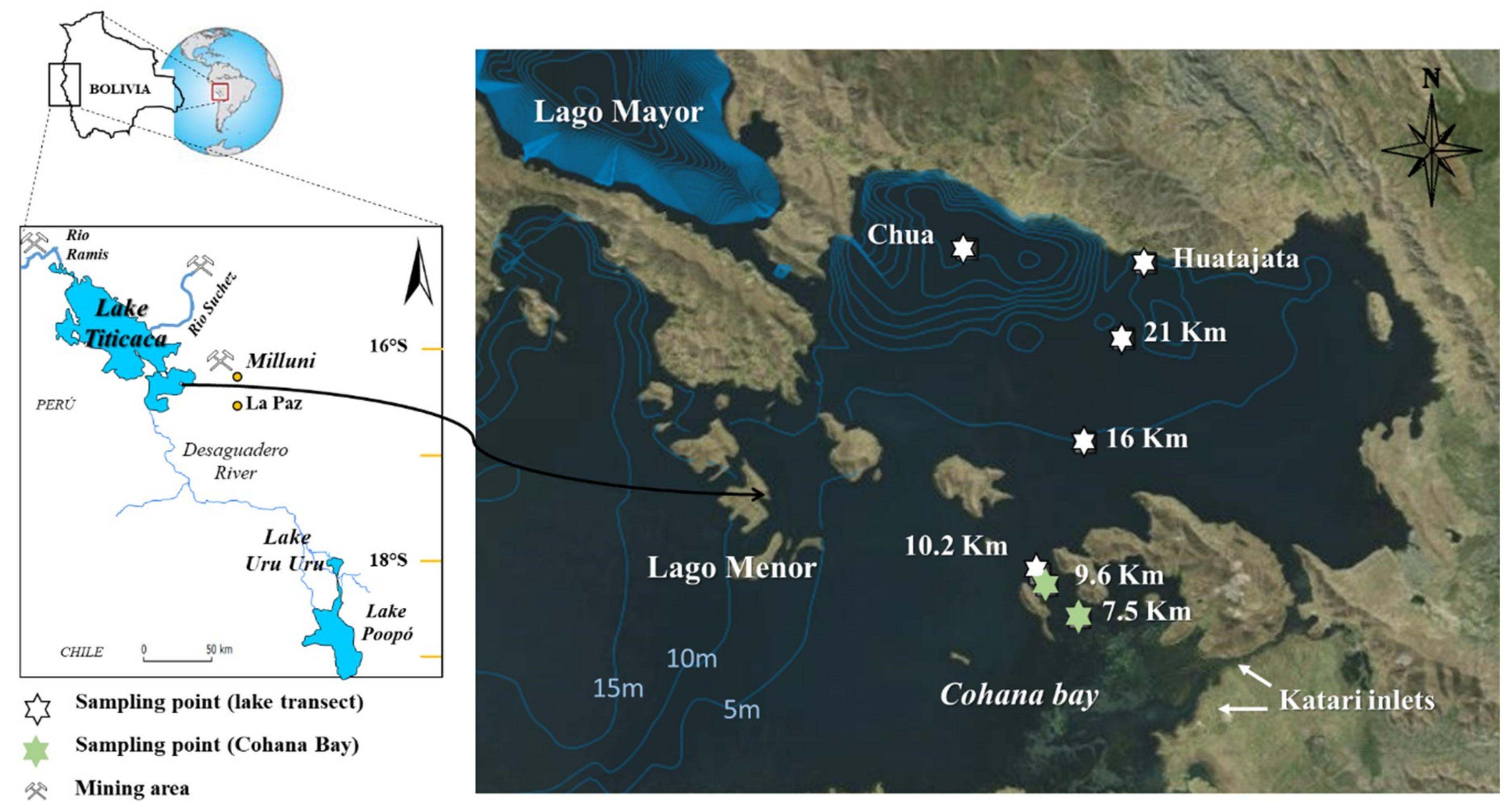
2.1. Study Area and Sampling

Lake Titicaca is the largest and most emblematic freshwater lake in South America located at 3809 m.a.s.l. on the Andean Altiplano (Perú-Bolivia) [54]. During the 1980’s the Lake Titicaca was a cold, oligotrophic lake [55]. Although its largest and deepest northern basin (Lago Mayor—7131 km2; mean depth = 100 m; max depth = 285 m) remains oligotrophic, there is growing evidence of rising eutrophication related to untreated domestic, industrial and agricultural wastewater discharges [56] in the southern shallow basin (Lago Menor—1428 km2; mean depth = 9 m; max depth = 40 m). Significant differences with the largest northern part of the lake in volume (12 vs. 900 km3) and depth (9 vs. 100 m), make Lago Menor more susceptible to eutrophication and global changes [57]. As a result, small portions of the lake are now eutrophic (i.e., mainly shallow bays). The study was conducted on Lago Menor (Figure 1, Table S1).
Owing to its tropical (~16°S) and high-altitude location, Lake Titicaca physicochemical characteristics are atypical. Dissolved oxygen saturation at 100% at such altitude is around 60% (6 mg∙L−1 at 15 °C) of the saturation at sea level (10 mg∙L−1 at 15 °C) [58]. UVA and UVB radiation levels in the lake are incredibly high, and photoinhibition impacts algae and other groups [59,60]. Evaporation (~90% of total lake output) dominates Lake Titicaca hydrological regime [37], and precipitation increase during the rainy season (December to March). The diurnal temperature cycle is wide-ranging (−20 to +20 °C) [61].
Due to its shallow water column, the entire water column of Lago Menor is mixed due to strong winds on a daily basis. The lake has a moderate salinity (0.810 ± 0.001) and is rich in sulfate (150–200 mg∙L−1, [56]) due to the geological context and mining activities of sulfide containing ores in the area. The pH is slightly alkaline (8.69 ± 0.02). Most littoral is dominated by macrophyte Totora (Schoenoplectus californicus), and the sediments of most of the shallow parts (<15 m) of the open lake were covered by the macroalgae Chara (Chara sp.). The main tributaries of Lago Menor are the Lago Mayor and the Katari River. The Katari River drain the densely populated area of El Alto city and discharges nutrients and contaminants into the Cohana Bay (Figure 1).
Sampling was conducted in April and October, at the end of the rainy season and the dry season respectively, from 2013 to 2016. Samples were collected along two transects; (i) in the open waters of the lake from the entrance Cohana Bay to Huatajata before, during and after the bloom (Points 10.2–21 km; Figure 1) and (ii) a in the Cohana Bay from the Katari river inlet to the outlet of the Bay before the bloom in several seasons (Point 7.5 & 9.6 km; Figure 1). Additional samplings were also performed before and after the bloom event including sampling points inside Cohana Bay, at Huatajata (24 km from Katari River inlet) and Chua (Figure 1).
Surface water (top 10 cm) was collected to identify algae responsible for the bloom, and for the measurement of major nutrients, dissolved organic carbon (DOC), mercury, MMHg, and hydrogen sulfide (H2S) during April 2015.

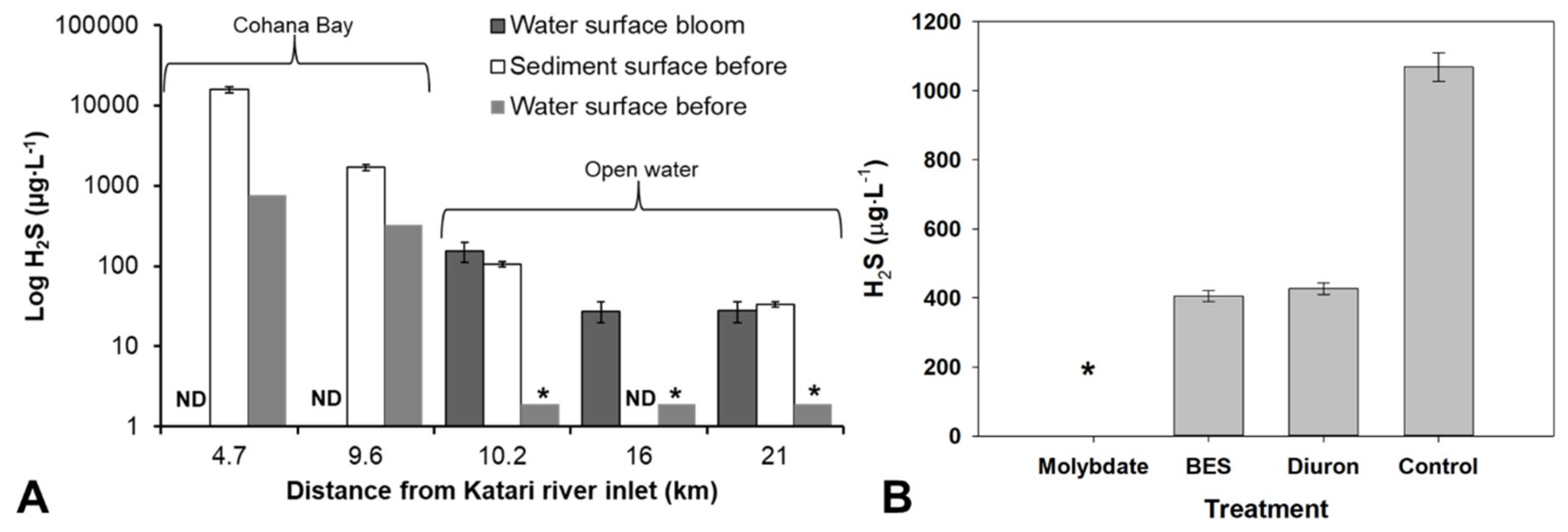
2.2. Hydrogen Sulfide

Samples for H2S were collected in triplicate directly into a degassed vacuum container, previously filled with 0.5 mL of a diamine mixture prepared as recommended [62]. Tubes with only diamine mixture were brought back to the lab to be later filled with ultrapure water and serve as field blanks. At a pH 7.8 and 9.2, most H2S in the lake was probably as HS-, but the method measured both species because the reaction with the diamine took place at very low pH. The diamine mixture was prepared with 50% concentrated hydrochloric acid. Hydrogen sulfide was determined using a modification of methods described elsewhere [63,64]. Briefly, 20 µL of the sample with the diamine mixture was injected into an Agilent 12600 HPLC with a Poroshell 120 EC-C18 Agilent column with a mix of 20% acetonitrile, 18% methanol, 20% sodium acetate buffer (pH 5.2, 0.05 mM) at 35 °C and 1.1 mL∙min−1. Concentrations were determined using the Radiello® (Millipore Sigma, Institi Clinici Scientifici Maugeri, Pavia, Italy) calibration solution for H2S Code 171. The relative standard deviation (RSD) among field replicates was between 8 and 29%. The RSD for analytical replicates was always below 3%. Field blanks were read at the same time as samples and were used to determine detection and quantification limits.

2.3. Mercury and Methylmercury

Water samples for mercury and monomethylmercury were collected with a Teflon-coated Go-Flo trace metals sampler and filtered (0.45 μm PVDF) directly after sampling in acid-washed FEP Teflon containers acidified with HCl (0.5%, v/v, Ultrex grade—Baker). Total mercury concentrations (THg) in surface were determined by cold vapor atomic fluorescence spectrometry (CV-AFS) after conversion of all mercury species into Hg0 followed by detection using a Tekran® (Scarborough, ON, Canada) (Model 2500). All MMHg values here reported are for filtered samples. Filtered MMHg concentrations were analyzed using a purge and trap-gas chromatography-AFS analyzer (MERX System, Brooks Rand®, Seattle, WA, USA) after being derivatized at pH 4.0 using 180 μL of a daily prepared 1% sodium tetraethylborate solution [28,65]. Filtered MMHg contents for all samples were duplicated and quantified using the standard addition technique. The average difference between replicates was 6% and always below 10%.

2.4. Dissolved Organic Carbon and Algae Identification

Water samples for Dissolved Organic Carbon (DOC) were filtered as for Hg and collected in pre-burnt (550 °C) amber borosilicate vials. DOC concentrations were determined using a Non-Dispersive Infra-Red (NDIR) CO2 Shimadzu® (Kyoto, Japan) (Model VCSN) spectrometer after wet oxidation in a sodium persulfate solution at 100 °C. Water samples to identify the algae involved in the bloom were collected with 500 mL high-density pre-cleaned flasks. Samples were preserved with Lugol [66] and refrigerated in the dark until analysis. Identification was performed with light microscopy and using freshwater algae taxonomic keys [67,68].

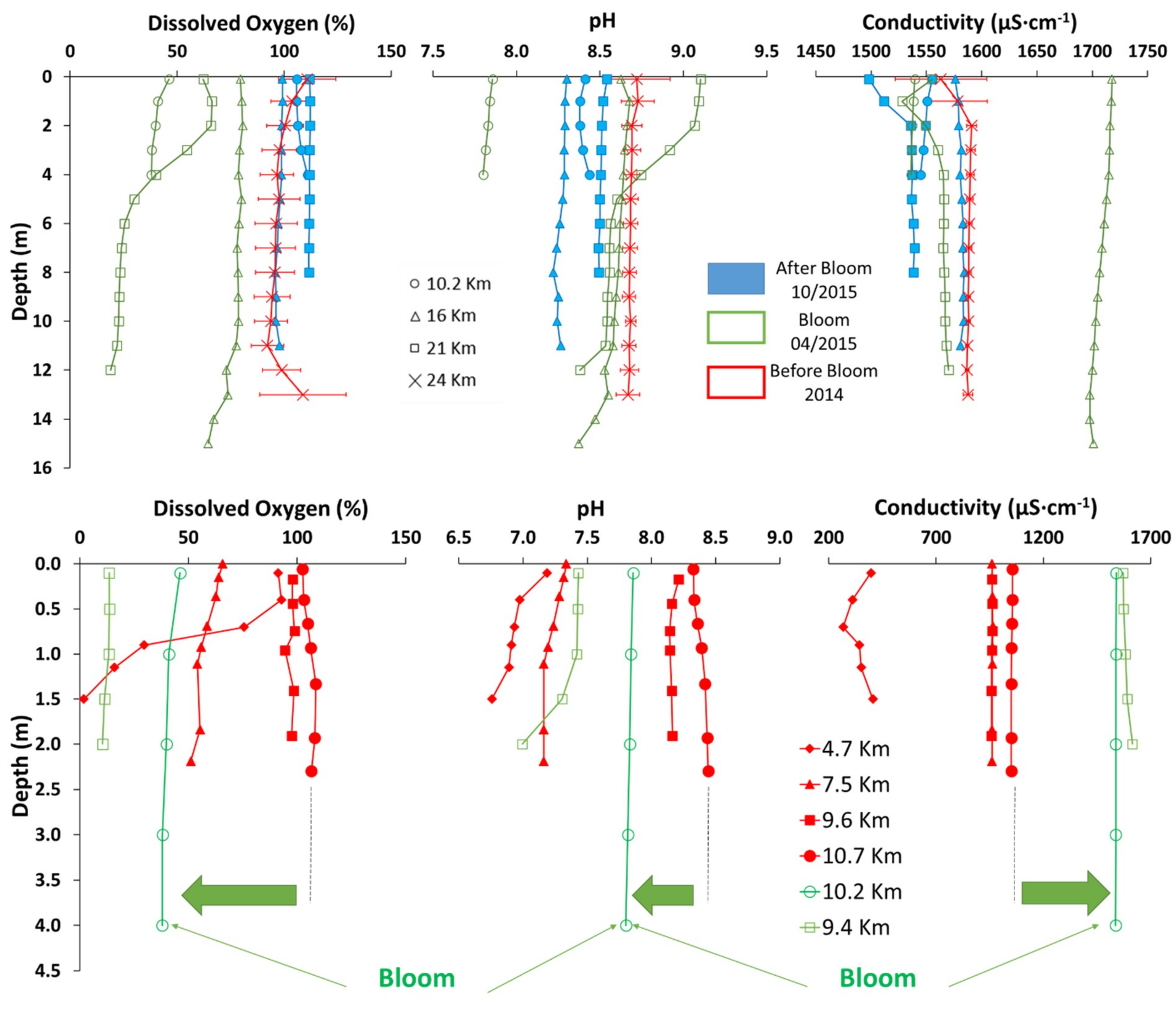
2.5. Water Column Characterization

A submersible multiparameter probe (HANNA HI-9828) (Hanna Instruments, Woonsocket, RI, USA) was used in each location to characterize the basic physicochemical conditions (pH, conductivity, dissolved oxygen concentration, oxygen saturation, and temperature). Data collection was conducted every three seconds for two minutes at the surface and then for one minute every 0.5 or 1 m. Values at each depth are the average of about 20 measurements. The same procedure was used in transects at Cohana bay in previous years. A subsample was sterilized by filtering through a 0.22 µm membrane into a polyethylene tube for nitrate and phosphate determinations. Anions were measured by ionic chromatography using a 332 Metrohm apparatus. Accuracy was evaluated with Carl Roth 2668.1 standard.

2.6. Incubation Experiments

Water and periphyton for incubation experiments were manually collected in polypropylene or Teflon flasks. Sediments (first 10 cm) were collected with a standard gravity corer. Samples were homogenized and distributed with similar weights for four treatments. Such treatments included a control sample and three samples amended with molybdate (sulfate-reducing bacteria inhibitor), BES (methanogenic bacteria inhibitor) and DIURON (photosynthesis inhibitor) respectively. Incubations lasted up to 24 h and then a water sample was collected from each flask containing either water, sediments or periphyton. Hydrogen sulfide determination followed the same protocol as for environmental water samples.

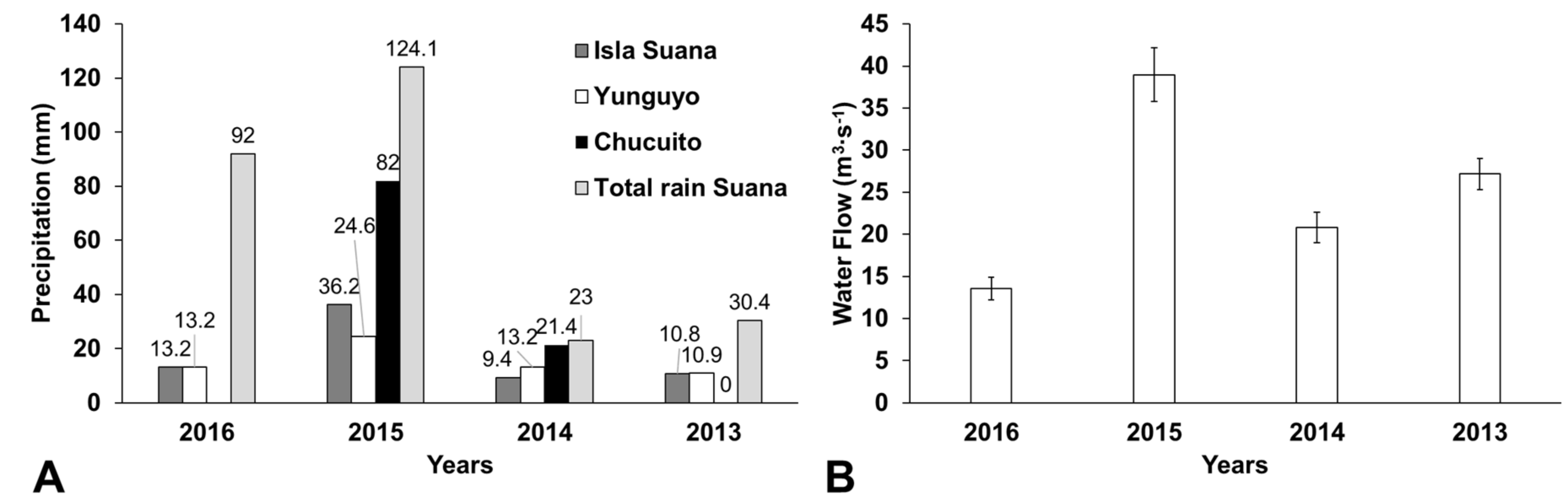
2.7. Climatological Data

The climatological data was collected from closer monitoring stations of Senamhi Perú as well as from a station set up by the French Institute of research for the development (IRD). Hour, daily, weekly averages and totals were compared from 2013 to 2016. The stations are close (20–100 m) to the shore.

2.8. Statistical Analysis

One-way ANOVA or Kruskal-Wallis one-way analysis was performed to compare physicochemical data from different locations and sampling periods, followed by multiple pairwise comparisons using Tukey test or Dunn’s Method respectively.

3. Results and Discussion

3.1. Algae Responsible for the Bloom and Consequences on Water Quality

The algae involved in the bloom was Carteria sp. since it represented nearly 100% of the algae in the water surface (first 10 cm) (Figure S1B). The species is probably Carteria multifilis because it has four equally sized flagella, contractile vacuole near the base of the flagellum and anterior eyespot (Figure S1A). Such algae is a relatively common free-living chlorophyte observed almost everywhere on the globe [69,70,71,72], but was never reported before in the Lake Titicaca. Nearby records include Brazil [73,74] and Argentina [69,75]. The genus was previously reported as the main algae involved in freshwater blooms [70,76]. From such algal growth in Lago Menor resulted in a major change in water geochemistry including oxygen drop that provoked more than two tons of aquatic biota death [77]. Oxygen saturation in the surface water and above sediments water during the day was above 100% (Figure 2 upper panels “X” symbol, Table S2) in the four years before the bloom. Such high oxygen saturation results from the presence of phytoplankton and mainly macrophytes (Chara sp.) in the shallow areas (<10 m depth) and abundant algae on surface sediment. However, during the bloom, surface water (~1 m below the water-air interface) oxygen saturations were significantly smaller (Kruskal-Wallis, p < 0.001) as low as 49% in shallow areas where Chara sp. dominates the lake bottom (i.e., 10.2 km; Figure 2). Such low oxygen saturations are only comparable to values observed near the sediments surface in the most polluted areas of Cohana Bay (2 to 51%) (Figure 2, lower panel). In Cohana Bay, average oxygen saturation in surface water in April 2014 (a year before the eutrophication event) was between 57% and 100% (Figure 2, lower panel). During the bloom and even though Carteria is photosynthetic, average oxygen saturation in the surface water dropped down to 13% and 28% (Figure 2, lower panel and Figure S2). Such changes are more significant at Lake Titicaca where oxygen saturation at 15 °C is about 6 mg∙L−1 than at close to sea level lakes where it would be 10 mg∙L−1 [58]. Life at Lake Titicaca had to evolve to tolerate naturally low oxygen concentration [78] but may be close to their limits in typical conditions, and anoxia alone may explain the death of organisms during the bloom.
Under normal conditions, pH and conductivity are stable throughout the lake and in-depth profiles (Figure 2, full blue symbols). During the bloom, changes in pH and conductivity were significant (Kruskal-Wallis, p < 0.001) (Figure 2, in pristine and weakly polluted areas) compared to values before and after the bloom, and differences were observed along the transect (Figure 2, empty green symbols). Surprisingly, changes in physicochemical water parameters during the bloom were completely different between the open lake and the Cohana Bay. In the middle of the lake, pH became alkaline (Kruskal-Wallis, p < 0.001) and rose up to 9, while at the entrance of the Cohana Bay pH became more acidic dropping down to ~7.8 (Figure 2). Similarly, conductivity increased (Kruskal-Wallis, p < 0.001) in the middle of the lake (Figure 2, squares and triangles), while it decreased at the entrance of the Cohana Bay (Kruskal-Wallis, p < 0.001).
Physicochemical data suggest additional water inputs into the lake before or during the bloom. Indeed, the Katari water, which flows into Cohana Bay, has a lower pH (6.7–7.4) and conductivity (431 to 614 μS∙cm−1) than the lake (pH: 8.2–8.7; EC: 1115 to 1598 μS∙cm−1), and consequently can explain acidification near Cohana Bay (Figure 2). Measured higher conductivity and pH in the open lake likely result from the runoff waters during heavy rains that leached the surrounding fields of the lake, or from sediment resuspensions. Our climatological data support the first hypothesis, precipitation during the bloom was much higher than previous and later years (Figure 3). At the same time, no significant difference was observed in the wind that could have explained sediment resuspension.

3.2. The Trigger Mechanism of the Bloom and Its Impact on Water Column Quality

The trigger mechanism of such algal bloom is likely related to nutrient inputs to the lake combined with the propitious climatic condition that allowed their spreading at the lake scale. According to nutrient inputs, the three likely candidates are (i) the Katari River which provides nutrients from the upstream urban area (i.e., wastewater), (ii) agricultural fields around the lake that are amended with fertilizers and (iii) sediment resuspension in the shallower (<5 m depth) parts of the lakes.
The Katari River is the main tributary of Lago Menor, which provides significant amounts of nutrients to the lake. Indeed, the little to no treatment of the sewage water originating from the upstream El Alto city is discharged in the Cohana Bay which is eutrophicated most of the year. In such a context of urban contamination and eutrophication, Cohana Bay is a great candidate to explain the bloom in Lago Menor [5,50]. Nutrient concentrations in the water column of the Cohana Bay were between 0.018 and 0.037 µmol∙L−1 of free phosphate and 0.43 and 5.23 µmol∙L−1 of nitrate. However, during the bloom phosphorus concentrations were at least one order of magnitude lower, maybe because most was already incorporated by algae. DOC was up to three-fold higher during the bloom (8.2 ± 5.0 mg∙L−1) than before the bloom (4.3 ± 1.5 mg∙L−1), but the variability between each sampling location was too high to get an average significant difference. However, physicochemical data between the open lake (Figure 2, upper panel) and the Cohana Bay (Figure 2, lower panel) suggest other sources of nutrients to the lake before or during the bloom than the Katari river. In general, conductivity (1557.5 ± 9.6 µS∙cm−1) and pH (8.38 ± 0.04) are pretty stable throughout the open lake profiles (Figure 2, full blue symbols and X symbols) and similar to the outer points of Cohana Bay transect (8.39 ± 0.04, Figure 2, lower panel red full circle). However, during the bloom, changes in pH (to 8.71 ± 0.13, 8.59 ± 0.04 or 7.83 ± 0.02) and conductivity (to 1561.1 ± 6.2, 1707 ± 3.5 or 1537 ± 1.2 µS cm−1) in open lake were significant (Kruskal-Wallis, p < 0.001) (Figure 2, empty green symbols) with some profiles going further away from the observed pH and Conductivity at Cohana Bay (Figure 2, lower panel red full symbols). Even the closest point to Cohana Bay from the open lake transect (Figure 2, empty green symbols) deviate significantly from the pH (from 8.39 ± 0.04 to 7.83 ± 0.02) and conductivity (from 1537 ± 1.2 to 1052.5 ± 1.9 µS∙cm−1) at the equivalent point of the Cohana Bay transect before the bloom (Figure 2, full red symbol).
Higher conductivity and pH in open lake during the bloom (Figure 2, green empty triangles and squares) may originate from the leaching of the surrounding fields of the lake by runoff during heavy rains [55,79]. Both acidification and alkalinization are possible consequences of nutrient enrichment [80], or algae blooms [81,82,83]. Carbon-rich nutrient inputs stimulate respiration, like those from Katari river, and consequently result in acidification while high algae CO2 consumption when photosynthesis is exacerbated rises pH [82,83,84]. Consequently, acidification near Cohana Bay (Figure 2, lower panel) could be the result of higher DOC concentrations, while alkalization of the rest of the lake could be associated to biological or abiotic CO2 depletion as a result of nutrients leaching from the surroundings (Figure S4). This hypothesis is also supported by conductivity data (Figure 2) and our climatological data which show that precipitation during the bloom was much higher than previous and later years (Figure 3).
Indeed, available climatological data from Lake Titicaca show that 2015 was a year with some unusually high precipitation events at the onset of the bloom (Figure 3). Total accumulated rain for April (124 mm) was 35% to 540% higher than other years between 2013 and 2016 (23 to 92 mm). Continuous rain events during April 2015 were between 2.7 and 3.8 times higher than other years at the same periods, increasing about two-fold in water overflowing at Desaguadero River (Figure 3B) compared to other years. Hence, total rain or recurrent extreme rain events have suggestively favored the dispersal of nutrients that triggered the bloom; Cohana Bay may have been flushed into the great lake, and agricultural soils bordering the lake have also suggestively been leached into the lake. Still, Cohana Bay does not seem to be the only responsible for nutrient enrichment, the bay itself did not present evidence of bloom as it can be observed in the satellite pictures (Figure S5).
Another plausible explanation for triggering of the bloom is sediment resuspension, which was shown to mobilize stocked nutrients [85]. Such a hypothesis agrees with satellite images that show the higher intensity of the bloom in the shallower parts of the lake (Figure S5). Sediment resuspension may also explain lake alkalization by CO2 consumption and calcium carbonate precipitation [84]. Sediment could also be important source phosphorus to the system because of sediment resuspension and changing redox conditions [85,86,87]. However, there was no significant difference (Kruskal-Wallis, H = 2.180, p = 0.536) in the daily average wind in March or April (2013–2017) that could have explained sediment resuspension and we do not have enough evidence to exclude or confirm that such process was involved in the bloom.
Regardless of the triggering mechanism of the bloom, our data shows that the lake Titicaca is more sensitive to nutrient enrichment and climate change than other lakes at lower altitudes or temperate systems. Smaller concentrations of nutrients seem to be enough to disrupt the system balance compared to other systems [84,86,88], and its high altitude implies already limited dissolved CO2 and O2 which makes it more susceptible to alkalization and hypoxia.

3.3. Algal Bloom Exacerbate the Production of H2S by Sulfate-Reducing Bacteria

In parallel to oxygen drop, the most striking feature of the bloom is the high hydrogen sulfide (H2S) concentrations measured in surface water at the open water transect, reaching up to 155 µg∙L−1 at (10.2 km—Figure 4A) during the bloom. H2S production in the lake is not surprising since the natural dissolved sulfate background is high (about 220 mg∙L−1) in Lake Titicaca. In Cohana Bay, higher H2S concentrations (from 1700 to 15,800 µg∙L−1) than in open water (from 33 to 106 µg∙L−1) were measured in surface sediments and water column before the bloom (Figure 4A). Such abrupt rise in H2S concentrations in surface water during the bloom likely result from two possible reasons or their combination; (i) the reduction or inhibition of H2S oxidation due to a drop in dissolved oxygen [88,89,90] or sulfur oxidizer inhibition, and (ii) changes in physicochemical conditions and ecological communities during the bloom that favored sulfate reducers.
The primary source of H2S in the open lake was the sediment-water interface (SWI) and the epibenthic biofilms where high H2S concentrations (i.e., up to 105 and 8450 µg∙L−1 at SWI and in biofilms, respectively) were detected outside of the bloom event. According to our incubation experiments with specific inhibitors for sulfate-reducing bacteria (SRB) (molybdate) [19], methanogen (BES) and photosynthesis (Diuron), H2S is produced mainly by SRB (Figure 4B). Partial inhibition with BES and Diuron suggests that at least part of the SRB activity is linked to syntrophic growth with methanogens and photosynthetic activity respectively. However, in normal conditions, H2S is always below the detection limit (i.e., <1.9 µg∙L−1) in the water column, probably because it is oxidized by dissolved oxygen [88,89,91] produced by Charophytes. Wild rice was shown to decrease H2S concentrations in mesocosm experiments [92]. However, the kinetics of abiotic H2S oxidation is slow [90,93], and sulfide-oxidizing bacteria are more likely to be responsible for H2S concentrations [90,94] than abiotic oxidation.
During the bloom, H2S concentrations in the surface water of the open lake (70 µg∙L−1) were comparable to those measured at the SWI before the bloom (Figure 4A), which represents an increase of ~35-fold baseline levels. Low oxygen conditions and availability of organic matter may have allowed more H2S production and even migration of SRB from the sediments to the water column. Carteria sp. biomass was reported to stimulate SRB and H2S production [1]. The biomass of other chlorophytes was also shown to stimulate sulfate reduction [1,2]. However, the peak in H2S was concomitant with the bloom, so it did not result from a late degradation of the biomass after settling at the bottom of the lake. We propose that the algal bloom creates a shield to the light, and inhibits the photosynthesis by Characea as well as photosynthetic H2S oxidation, preventing abiotic and biotic H2S oxidation (Figure S4).
Such an abrupt rise of H2S had a toxic effect on the lake’s biota. Some H2S values were above the WHO criteria of 50 µg∙L−1 for drinking water [95] and all above the US-EPA criterion of 2 µg∙L−1 for freshwater fish and another biota [96]. H2S is toxic for almost all types of aquatic organisms, although some species have developed tolerance mechanisms [97,98]. Values below 130 µg∙L−1 are toxic for marine invertebrates [99,100]. LC50 values for H2S range from 0.002 to 6 mg∙L−1 were reported mostly for sediment invertebrates [100,101]. Toxicity of H2S for plants was also observed (0.170–49.075 mg∙L−1), with a variety of effects on macrophytes [100,102]. At high concentrations, H2S has been shown to be the main factor for macrophyte distribution [102]. Such toxicity may have a synergistic effect with eutrophication effects on reduction of oxygen concentrations in the water column and on the release of more nitrogen and phosphorous to the water column [92].

3.4. Enhanced Methylmercury Concentration in Surface Water during the Bloom

Total mercury (THg) level in Lake Titicaca is relatively low in the open water and a bit higher in Cohana Bay [57]. Although the main anthropogenic source of Hg is likely to be the Cohana Bay, both the Totora barrier [103,104] and the dilution effect is sufficient to rapidly reach a baseline concentration of <1 ng∙L−1 few km away from the Katari inlet (Figure 5B). Higher sulfate reduction in the system may explain the increase of Hg in the water column [92]. Although MMHg is also low in concentration, a striking feature is a high percentage in MMHg which rises up to 20% while in non-contaminated surface waters around the globe it generally stands around 1–2%. As discussed in a previous publication [57], these high MMHg percentages can be explained by (i) high MMHg production in an environment favorable to methylating micro-organisms (e.g., sulfate-rich water and sediment, lower dissolved oxygen levels, neutral to alkaline water, shallow areas, et al.) [92], (ii) stabilization and accumulation of MMHg in waters due to abundant (in)organic ligands [105], and (iii) low degradation of MMHg in organic-rich waters.
Filtered MMHg concentration in water increased at all sampled locations (up to 2.6 times) during the bloom (Figure 5A) compared to before and after the event. This rise is even more significant if we consider the dilution effect at the time of the bloom (i.e., end of the rainy season) compared to concentrations measured during the dry season (September or October) outside of the bloom (Figure 5D). These higher MMHg concentrations during the bloom are consistent with observed higher MMHg concentrations (51 pg∙L−1) found in the eutrophicated Cohana Bay compared to the open lake water (27 pg∙L−1) out of the bloom event. We also reported the same pattern for different lakes having contrasted trophic states in the TDPS system were the most eutrophicated areas showed the highest MMHg values [57].
In the case of the bloom, the large biomass generated by the algae forming the bloom should have up taken large amounts of MMHg since chlorophytes were shown to bioaccumulate large quantities of MMHg [104]. During the algal bloom, an average of 48% of THg (up to 69%) was found on the fraction > 0.45 µm (i.e., unfiltered minus filtered fraction), while after the bloom (i.e., October) only 18% of the THg was encountered in the filtered phase (i.e., truly dissolved and adsorbed on colloids). In addition, MMHg concentrations measured at Cohana Bay, Huatajata and Chua (Figure 1) during the years before the bloom showed that an average of 43% of total MMHg and 54% of THg was found in the filtered fraction [57]. Therefore, the total MMHg increase (i.e., particulate and filtered) in the system during the bloom is underestimated at least by a factor of 2 since we only measured MMHg concentrations in filtered water.
High sulfate levels in the systems that prompt SRB dominance under low oxygen conditions, as shown by the high H2S concentrations, may explain the observed increase of MMHg in the water [92]. SRB are the main Hg methylators at Titicaca Lake [105]. However, several studies have suggested that blooms may reduce MMHg concentrations in algae by a biomass growth dilution effect and have shown observationally [106] and experimental data [6,7,107] to support such a hypothesis. However, a recent modeling work showed that under some conditions, algae blooms might stimulate MMHg production by stimulating SRB activity [108]. So, our results support such recent modeling projections (Figure 5A). It seems that under sulfate-rich conditions a bloom generates the ideal conditions for SRB, the principal Hg methylators [105], to thrive and generate not only high H2S concentrations but also higher MMHg concentrations. The effect of the bloom on the oxygen profile (Figure 2) may have allowed SRB to move the periphyton and biofilms associated with sediments [105] to the water column. Also, abundant ligands present in these alkaline waters have likely favored the stabilization of MMHg in surface waters [57].
During the bloom, radiations were strongly reduced due to the presence of high DOC, suspended particulate matter (mostly dominated by algae) which contributed themselves to the UV absorption. Indeed, in normal conditions, UVA and UVB radiations are extremely high at this altitude favoring both photoinhibition of phytoplankton (so most algae are absent in the first 4–8 m below the surface), and photodemethylation [59,60]. Hence, this barrier to UVs has likely inhibited much of MMHg photodemethylation [109], which contributed to elevated MMHg concentrations in water.
Although a good correlation (R = 0.95, p < 0.001—Figure 5B) is found between THg and the distance from the Katari River inlet, showing that inorganic Hg enters the lake at Cohana Bay, there was no significant increase in THg during the bloom (p > 0.05) compared to before the bloom (Figure S6). The absence of THg increase suggests that the increase of MMHg was only the result of changes in Hg methylation and demethylation rates. The leaching of coastal areas may also increase the releases of inorganic Hg, but usually, the Totora blocks the sedimentation at >95%. Even more, an increase in the percentage of MMHg at all sampling locations was also observed during the bloom (Figure 5C). Consequently, our data suggest bloom events, which are likely to reoccur, may increase MMHg contamination in the food web as well as risk for human exposure.
After the bloom, MMHg concentrations declined to levels below those observed before the bloom (Figure 5C). MMHg may have precipitated with the organic matter from the decaying algae bloom. At the same time pH, oxygen and conductivity returned to baseline levels, which show the resilience of the system to the bloom consequences. However, nutrients that caused the bloom are now mostly deposited in the sediments where they may get re-suspended. Additionally, the macrophyte community may have declined due to the toxicity of hydrogen sulfide [102], which makes sediment more susceptible to resuspension as well as future bloom events.

4. Conclusions and Perspectives

Overall our results suggest that the first ever recorded massive bloom in Titicaca was triggered by extreme climatological events that enhanced nutrient fluxes from both the Katari River and agricultural field bordering the lake. The formation of a shield to UV by the Carteria inhibited the photosynthesis by macrophytes (mainly Chara), so dissolved oxygen dropped, possibly inhibited photosynthetic H2S oxidizers and H2S was not oxidized and diffused in the whole water column. The resulting consequence was pronounced anoxia and particularly the production of large amounts of H2S which was the most harmful consequence of the bloom for aquatic biota. In parallel, due to the high sulfate content of the lake, the enhanced activity of SRBs and the absence of photodemethylation, MMHg concentration increased in surface water. Our results show that sulfate reduction is a driving force on the effects of nutrient enrichment at this naturally sulfur enriched environment, as suggested by previous mesocosm experiments [92]. The whole process is synthesized in Figure S4.
Extreme climatological events may be more frequent in the future because of climate change [46]. Besides the trigger of an algae bloom, it is clear that there is a strong relationship between such events and chronic eutrophication processes. Even more, our data suggest that high altitude or sulfate enriched lakes have a specific sensitivity to eutrophication or algae blooms, and consequently their unique biodiversity is more vulnerable to such events. Although, our data show a significant recovery of water quality, recovery of natural populations is less likely to be as fast or as complete as chemical conditions.

Supplementary Materials

The following are available online at https://www.mdpi.com/2076-3263/8/12/438/s1, Figure S1: Algae responsible for the bloom at different scales showing the dominance of Carteria sp. at the water surface. (A), and one of the images used for classification (B); Figure S2. Oxygen profiles of the water column in the Cohana Bay during the bloom 8:30 in the morning (circles) and 17:30 (tringles); Figure S3. Location of meteorological stations from where data was collected by Senamhi Peru (green circles) and IRD France (Blue circle) (modified from the map provided by Senamhi Peru, http://www.senamhi.gob.pe/); Figure S4. Diagram of the Titicaca Lake ecosystem under (A) undisturbed conditions, (B) bloom close to Cohana Bay and (C) bloom at open waters. Shows how the bloom may have allowed higher hydrogen sulfide concentrations, higher Sulfate-reducing bacteria (SRB) activity, higher methylmercury (CH3Hg2+) concentrations and how organic matter (OM) consumption and decomposition lowers or increases pH respectively; Figure S5. Satellite images showing the lake Menor of Titicaca during the bloom event. Upper panel with a. Landsat 8 image 23-04-2015 and in the bottom panel from blue to red gradient showing Chlorophyll content of the same image (modified from Earth Observation Services Supporting International Development Banks Projects (EOSID), project developed and funded by the European Space Agency (ESA) under ESA Earth Observation Envelope Programme). Note that the view expressed in this publication can in no way be taken. to reflect the official opinion of the European Space Agency. Figure S6. Total mercury concentrations in filtered water (THgF) in the, 21, 16 and 10.2 km sampling locations during (green circles), before (red squares) and after the algae bloom (blue triangles); Table S1: Main sampling locations at Lago Menor; Table S2: Oxygen concentrations during the bloom.

Author Contributions

The conceptualization, D.A. (Darío Achá) and S.G.; methodology, D.A. (Darío Achá), S.G., D.A. (David Amouroux), D.P.; formal analysis, D.A. (Darío Achá), S.G., G.S., X.L. and P.E.F.; investigation, D.A. (Darío Achá), S.G. and G.S.; resources, G.S., S.G., D.A. (David Amouroux) and D.A. (Darío Achá); data curation, D.A. (Darío Achá), S.G. and G.S.; writing—original draft preparation, D.A. (Darío Achá); writing—review and editing, S.G., G.S., X.L., D.A. (David Amouroux), D.P.; project administration, G.S., D.A. (Darío Achá), S.G.; funding acquisition, G.S., S.G., D.A. (Darío Achá) and D.A. (David Amouroux).

Funding

This work was supported by the LATICO2 project, which was funded by IDH (Impuesto directo a los hidrocarburos) at Universidad Mayor de San Andres, as well as, by the Swedish International Development Cooperation Agency (SIDA)—Bolivia through the “Water pollution and remediation” project at UMSA. TRACISOMER supported by a grant from Labex OSUG@2020 (Investissements d’avenir—ANR10 LABX56, PI: S. Guédron: [email protected]). This work was also supported by the project "PHYTOBOL" funded by EC2CO program (CNRS, INSU) (P.I. Géraldine Sarret). This work is also a contribution to the LA PACHAMAMA project (ANR CESA program, No 423 ANR-13-CESA-0015-01, PI: D. Amouroux: [email protected]), and to the “Identificación de Bioindicadores de cambio climático en lagos emblemáticos del Altiplano Boliviano” project (PIA-ACC, UMSA20: COSUDE).

Acknowledgments

We thank the IRD and especially Franck Timouk for providing important supplementary climatological data.

Conflicts of Interest

The authors declare no conflict of interest.

References

  1. Smith, V.H. Eutrophication of freshwater and coastal marine ecosystems: A global problem. Environ. Sci. Pollut. Res. 2003, 10, 126–139. [Google Scholar] [CrossRef]
  2. Fey, S.B.; Siepielski, A.M.; Nusslé, S.; Cervantes-Yoshida, K.; Hwan, J.L.; Huber, E.R.; Fey, M.J.; Catenazzi, A.; Carlson, S.M. Recent shifts in the occurrence, cause, and magnitude of animal mass mortality events. Proc. Natl. Acad. Sci. USA 2015, 112, 1083–1088. [Google Scholar] [CrossRef] [PubMed] [Green Version]
  3. Paerl, H.W.; Huisman, J. Blooms Like It Hot. Science 2008, 320, 57–58. [Google Scholar] [CrossRef] [PubMed]
  4. Havens, K.E. Cyanobacteria blooms: Effects on aquatic ecosystems. In Cyanobacterial Harmful Algal Blooms: State of the Science and Research Needs; Hudnell, H.K., Ed.; Springer: New York, NY, USA, 2008; pp. 733–747. [Google Scholar]
  5. Anderson, D.M.; Glibert, P.M.; Burkholder, J.M. Harmful algal blooms and eutrophication: Nutrient sources, composition, and consequences. Estuaries 2002, 25, 704–726. [Google Scholar] [CrossRef]
  6. Pickhardt, P.C.; Folt, C.L.; Chen, C.Y.; Klaue, B.; Blum, J.D. Algal blooms reduce the uptake of toxic methylmercury in freshwater food webs. Proc. Natl. Acad. Sci. USA 2002, 99, 4419–4423. [Google Scholar] [CrossRef] [PubMed] [Green Version]
  7. Walters, D.M.; Raikow, D.F.; Hammerschmidt, C.R.; Mehling, M.G.; Kovach, A.; Oris, J.T. Methylmercury Bioaccumulation in Stream Food Webs Declines with Increasing Primary Production. Environ. Sci. Technol. 2015, 49, 7762–7769. [Google Scholar] [CrossRef] [PubMed]
  8. Ayala-Parra, P.; Sierra-Alvarez, R.; Field, J.A. Algae as an electron donor promoting sulfate reduction for the bioremediation of acid rock drainage. J. Hazard. Mater. 2016, 317, 335–343. [Google Scholar] [CrossRef] [PubMed] [Green Version]
  9. Russell, R.A.; Holden, P.J.; Wilde, K.L.; Neilan, B.A. Demonstration of the use of Scenedesmus and Carteria biomass to drive bacterial sulfate reduction by Desulfovibrio alcoholovorans isolated from an artificial wetland. Hydrometallurgy 2003, 71, 227–234. [Google Scholar] [CrossRef]
  10. Parks, J.M.; Johs, A.; Podar, M.; Bridou, R.; Hurt, R.A.; Smith, S.D.; Tomanicek, S.J.; Qian, Y.; Brown, S.D.; Brandt, C.C.; et al. The Genetic Basis for Bacterial Mercury Methylation. Science 2013, 339, 1332–1335. [Google Scholar] [CrossRef] [PubMed]
  11. King, J.K.; Kostka, J.E.; Frischer, M.E.; Saunders, F.M. Sulfate-reducing bacteria methylate mercury at variable rates in pure culture and in marine sediments. Appl. Environ. Microbiol. 2000, 66, 2430–2437. [Google Scholar] [CrossRef] [PubMed]
  12. Watras, C.J.; Back, R.C.; Halvorsen, S.; Hudson, R.J.M.; Morrison, K.A.; Wente, S.P. Bioaccumulation of mercury in pelagic freshwater food webs. Sci. Total Environ. 1998, 219, 183–208. [Google Scholar] [CrossRef]
  13. Mason, R.; Reinfelder, J.; Morel, F. Bioaccumulation of mercury and methylmercury. Water Air Soil Pollut. 1995, 80, 915–921. [Google Scholar] [CrossRef]
  14. Watanabe, C.; Satoh, H. Evolution of our understanding of methylmercury as a health threat. Environ. Health Perspect. 1996, 104, 367–379. [Google Scholar] [PubMed]
  15. Yokoo, E.M.; Valente, J.G.; Grattan, L.; Schmidt, S.L.; Platt, I.; Silbergeld, E.K. Low level methylmercury exposure affects neuropsychological function in adults. Environ. Health 2003, 2, 8. [Google Scholar] [CrossRef] [PubMed] [Green Version]
  16. Gilmour, C.C.; Podar, M.; Bullock, A.L.; Graham, A.M.; Brown, S.D.; Somenahally, A.C.; Johs, A.; Hurt, R.A.; Bailey, K.L.; Elias, D.A. Mercury Methylation by Novel Microorganisms from New Environments. Environ. Sci. Technol. 2013, 47, 11810–11820. [Google Scholar] [CrossRef] [PubMed] [Green Version]
  17. Compeau, G.C.; Bartha, R. Sulfate-reducing bacteria: Principal methylators of mercury in anoxic estuarine sediment. Appl. Environ. Microbiol. 1985, 50, 498–502. [Google Scholar] [PubMed]
  18. Hellal, J.; Guédron, S.; Huguet, L.; Schafer, J.; Laperche, V.; Joulian, C.; Lanceleur, L.; Burnol, A.; Ghestem, J.P.; Garrido, F.; et al. Mercury mobilization and speciation linked to bacterial iron oxide and sulfate reduction: A column study to mimic reactive transfer in an anoxic aquifer. J. Contam. Hydrol. 2015, 180, 56–68. [Google Scholar] [CrossRef] [PubMed]
  19. Fleming, E.J.; Mack, E.E.; Green, P.G.; Nelson, D.C. Mercury Methylation from Unexpected Sources: Molybdate-Inhibited Freshwater Sediments and an Iron-Reducing Bacterium. Appl. Environ. Microbiol. 2006, 72, 457–464. [Google Scholar] [CrossRef] [PubMed] [Green Version]
  20. Hamelin, S.P.; Amyot, M.; Barkay, T.; Wang, Y.; Planas, D. Methanogens: Principal Methylators of Mercury in Lake Periphyton. Environ. Sci. Technol. 2011, 45, 7693–7700. [Google Scholar] [CrossRef] [PubMed]
  21. Achá, D.; Pabón, C.A.; Hintelmann, H. Mercury methylation and hydrogen sulfide production among unexpected strains isolated from periphyton of two macrophytes of the Amazon. FEMS Microbiol. Ecol. 2012, 80, 637–645. [Google Scholar] [CrossRef] [PubMed] [Green Version]
  22. Eckley, C.; Watras, C.J.; Hintelmann, H.; Morrison, K.; Kent, A.D.; Regnell, O. Mercury methylation in the hypolimnetic waters of lakes with and without connection to wetlands in northern Wisconsin. Can. J. Fish. Aquat. Sci. 2005, 62, 400–411. [Google Scholar] [CrossRef] [Green Version]
  23. Watras, C.J.; Bloom, N.S.; Claas, S.A.; Morrison, K.A.; Gilmour, C.C.; Craig, S.R. Methylmercury production in the anoxic hypolimnion of a Dimictic Seepage Lake. Water Air Soil Pollut. 1995, 80, 735–745. [Google Scholar] [CrossRef]
  24. Compeau, G.C.; Bartha, R. Effect of Salinity on Mercury-Methylating Activity of Sulfate-Reducing Bacteria in Estuarine Sediments. Appl. Environ. Microbiol. 1987, 53, 261–265. [Google Scholar] [PubMed]
  25. Gilmour, C.C.; Henry, E.A.; Mitchell, R. Sulfate Stimulation of Mercury Methylation In Freshwater Sediments. Environ. Sci. Technol. 1992, 26, 2281–2287. [Google Scholar] [CrossRef]
  26. Guimarães, J.R.D.; Roulet, M.; Lucotte, M.; Mergler, D. Mercury methylation along a lake-forest transect in the Tapajós river floodplain, Brazilian Amazon: Seasonal and vertical variations. Sci. Total Environ. 2000, 261, 91–98. [Google Scholar] [CrossRef]
  27. Desrosiers, M.; Planas, D.; Mucci, A. Mercury methylation in the epilithon of boreal shield aquatic ecosystems. Environ. Sci. Technol. 2006, 40, 1540–1546. [Google Scholar] [CrossRef] [PubMed]
  28. Guédron, S.; Grimaldi, M.; Grimaldi, C.; Cossa, D.; Tisserand, D.; Charlet, L. Amazonian former gold mined soils as a source of methylmercury: Evidence from a small scale watershed in French Guiana. Water Res. 2011, 45, 2659–2669. [Google Scholar] [CrossRef] [PubMed]
  29. Mauro, J.B.; Guimaraes, J.R.; Hintelmann, H.; Watras, C.J.; Haack, E.A.; Coelho-Souza, S.A. Mercury methylation in macrophytes, periphyton, and water—Comparative studies with stable and radio-mercury additions. Anal. Bioanal. Chem. 2002, 374, 983–989. [Google Scholar] [PubMed]
  30. Acha, D.; Iniguez, V.; Roulet, M.; Guimaraes, J.R.; Luna, R.; Alanoca, L.; Sanchez, S. Sulfate-reducing bacteria in floating macrophyte rhizospheres from an Amazonian floodplain lake in Bolivia and their association with Hg methylation. Appl. Environ. Microbiol. 2005, 71, 7531–7535. [Google Scholar] [CrossRef] [PubMed]
  31. Molina, C.I.; Gibon, F.-M.; Duprey, J.-L.; Dominguez, E.; Guimaraes, J.R.D.; Roulet, M. Transfer of mercury and methylmercury along macroinvertebrate food chains in a floodplain lake of the Beni River, Bolivian Amazonia. Sci. Total Environ. 2010, 408, 3382–3391. [Google Scholar] [CrossRef] [PubMed]
  32. Hsu-Kim, H.; Eckley, C.S.; Achá, D.; Feng, X.; Gilmour, C.C.; Jonsson, S.; Mitchell, C.P.J. Challenges and opportunities for managing aquatic mercury pollution in altered landscapes. Ambio 2018, 47, 141–169. [Google Scholar] [CrossRef] [PubMed] [Green Version]
  33. Abbott, M.B.; Wolfe, B.B.; Wolfe, A.P.; Seltzer, G.O.; Aravena, R.; Mark, B.G.; Polissar, P.J.; Rodbell, D.T.; Rowe, H.D.; Vuille, M. Holocene paleohydrology and glacial history of the central Andes using multiproxy lake sediment studies. Palaeogeogr. Palaeoclim. Palaeoecol. 2003, 194, 123–138. [Google Scholar] [CrossRef]
  34. Bradley, R.S.; Vuille, M.; Diaz, H.F.; Vergara, W. Threats to Water Supplies in the Tropical Andes. Science 2006, 312, 1755–1756. [Google Scholar] [CrossRef] [PubMed]
  35. Vuille, M.; Francou, B.; Wagnon, P.; Juen, I.; Kaser, G.; Mark, B.G.; Bradley, R.S. Climate change and tropical Andean glaciers: Past, present and future. Earth Sci. Rev. 2008, 89, 79–96. [Google Scholar] [CrossRef]
  36. Perry, L.B.; Seimon, A.; Andrade-Flores, M.F.; Endries, J.L.; Yuter, S.E.; Velarde, F.; Arias, S.; Bonshoms, M.; Burton, E.J.; Winkelmann, I.R.; et al. Characteristics of Precipitating Storms in Glacierized Tropical Andean Cordilleras of Peru and Bolivia. Ann. Am. Assoc. Geogr. 2017, 107, 309–322. [Google Scholar] [CrossRef]
  37. Delclaux, F.; Coudrain, A.; Condom, T. Evaporation estimation on Lake Titicaca: A synthesis review and modelling. Hydrol. Process. 2007, 21, 1664–1677. [Google Scholar] [CrossRef]
  38. Weide, D.M.; Fritz, S.C.; Hastorf, C.A.; Bruno, M.C.; Baker, P.A.; Guédron, S.; Salenbien, W. A ~6000 yr diatom record of mid- to late Holocene fluctuations in the level of Lago Wiñaymarca, Lake Titicaca (Peru/Bolivia). Quat. Res. 2017, 88, 179–192. [Google Scholar] [CrossRef]
  39. Fritz, S.C.; Baker, P.A.; Tapia, P.; Spanbauer, T.; Westover, K. Evolution of the Lake Titicaca basin and its diatom flora over the last ~370,000 years. Palaeogeogr. Palaeoclimatol. Palaeoecol. 2012, 317–318, 93–103. [Google Scholar] [CrossRef]
  40. Cross, S.L.; Baker, P.A.; Seltzer, G.O.; Fritz, S.C.; Dunbar, R.B. Late Quaternary climate and hydrology of tropical South America inferred from an isotopic and chemical model of Lake Titicaca, Bolivia and Peru. Quat. Res. 2001, 56, 1–9. [Google Scholar] [CrossRef]
  41. Fritz, S.C.; Metcalfe, S.E.; Dean, W. Holocene climate patterns in the Americas inferred from paleolimnological records. In Interhemispheric Climate Linkages; Elsevier: San Diego, CA, USA, 2001; pp. 241–263. [Google Scholar]
  42. Baker, P.A.; Fritz, S.C.; Garland, J.; Ekdahl, E. Holocene hydrologic variation at Lake Titicaca, Bolivia/Peru, and its relationship to North Atlantic climate variation. J. Quat. Sci. Publ. Quat. Res. Assoc. 2005, 20, 655–662. [Google Scholar] [CrossRef] [Green Version]
  43. Francou, B.; Vuille, M.; Wagnon, P.; Mendoza, J.; Sicart, J.-E. Tropical climate change recorded by a glacier in the central Andes during the last decades of the twentieth century: Chacaltaya, Bolivia, 16°S. J. Geophys. Res. Atmos. 2003, 108, 4154. [Google Scholar] [CrossRef]
  44. Heidinger, H.; Carvalho, L.; Jones, C.; Posadas, A.; Quiroz, R. A new assessment in total and extreme rainfall trends over central and southern Peruvian Andes during 1965–2010. Int. J. Climatol. 2018, 38, e998–e1015. [Google Scholar] [CrossRef]
  45. Vera, C.; Silvestri, G.; Liebmann, B.; González, P. Climate change scenarios for seasonal precipitation in South America from IPCC-AR4 models. Geophy. Res. Lett. 2006, 33, L13707. [Google Scholar] [CrossRef]
  46. Fischer, E.M.; Knutti, R. Anthropogenic contribution to global occurrence of heavy-precipitation and high-temperature extremes. Nature Clim. Chang. 2015, 5, 560–564. [Google Scholar] [CrossRef]
  47. Paerl, H.W.; Paul, V.J. Climate change: Links to global expansion of harmful cyanobacteria. Water Res. 2012, 46, 1349–1363. [Google Scholar] [CrossRef] [PubMed]
  48. Whitehead, P.G.; Wilby, R.L.; Battarbee, R.W.; Kernan, M.; Wade, A.J. A review of the potential impacts of climate change on surface water quality. Hydrol. Sci. J. 2009, 54, 101–123. [Google Scholar] [CrossRef] [Green Version]
  49. O’Donnell, D.R.; Wilburn, P.; Silow, E.A.; Yampolsky, L.Y.; Litchman, E. Nitrogen and phosphorus colimitation of phytoplankton in Lake Baikal: Insights from a spatial survey and nutrient enrichment experiments. Limnol. Oceanogr. 2017, 62, 1383–1392. [Google Scholar] [CrossRef]
  50. Heisler, J.; Glibert, P.; Burkholder, J.; Anderson, D.; Cochlan, W.; Dennison, W.; Gobler, C.; Dortch, Q.; Heil, C.; Humphries, E.; et al. Eutrophication and Harmful Algal Blooms: A Scientific Consensus. Harmful Algae 2008, 8, 3–13. [Google Scholar] [CrossRef] [PubMed]
  51. Dale, B.; Edwards, M.; Reid, P.C. Climate Change and Harmful Algal Blooms. In Ecology of Harmful Algae; Granéli, E., Turner, J.T., Eds.; Springer: Heidelberg, Germany, 2006; pp. 367–378. [Google Scholar]
  52. Freitas, R.; Vieira, H.H.; de Moraes, G.P.; de Melo, M.L.; Vieira, A.A.H.; Sarmento, H. Productivity and rainfall drive bacterial metabolism in tropical cascading reservoirs. Hydrobiologia 2018, 809, 233–246. [Google Scholar] [CrossRef]
  53. Booth, S.; Zeller, D. Mercury, Food Webs, and Marine Mammals: Implications of Diet and Climate Change for Human Health. Environ. Health Perspect. 2005, 113, 521–526. [Google Scholar] [CrossRef] [PubMed] [Green Version]
  54. Ronchail, J.; Espinosa, J.C.; Labat, D.; Callede, J.; Lavado, W. Evolution of the Titicaca Lake level during the 20th century. In Línea Base de Conocimientos Sobre Los Recursos Hidrológicos e Hidrobiológicos en el Sistema TDPS con Enfoque en la Cuenca del Lago Titicaca; Aguirre, M., Pouilly, M., Lazzaro, X., Point, D., Eds.; UICN-IRD: La Paz, Bolivia, 2014; pp. 1–13. [Google Scholar]
  55. El Lago Titicaca: Síntesis del Conocimiento Limnológico Actual; Dejoux, C.; Iltis, A. (Eds.) ORSTOM—HISBOL: La Paz, Bolivia, 1991; p. 584. [Google Scholar]
  56. Archundia, D.; Duwig, C.; Spadini, L.; Uzu, G.; Guédron, S.; Morel, M.C.; Cortez, R.; Ramos Ramos, O.; Chincheros, J.; Martins, J.M.F. How Uncontrolled Urban Expansion Increases the Contamination of the Titicaca Lake Basin (El Alto, La Paz, Bolivia). Water Air Soil Pollut. 2017, 228, 44. [Google Scholar] [CrossRef]
  57. Guédron, S.; Point, D.; Acha, D.; Bouchet, S.; Baya, P.A.; Tessier, E.; Monperrus, M.; Molina, C.I.; Groleau, A.; Chauvaud, L.; et al. Mercury contamination level and speciation inventory in Lakes Titicaca & Uru-Uru (Bolivia): Current status and future trends. Environ. Pollut. 2017, 231, 262–270. [Google Scholar]
  58. Truesdale, G.A.; Downing, A.L.; Lowden, G.F. The solubility of oxygen in pure water and sea-water. J. Appl. Chem. 1955, 5, 53–62. [Google Scholar] [CrossRef]
  59. Villafañe, V.E.; Andrade, M.; Lairana, V.; Zaratti, F.; Helbling, E.W. Inhibition of phytoplankton photosynthesis by solar ultraviolet radiation: Studies in Lake Titicaca, Bolivia. Freshw. Biol. 1999, 42, 215–224. [Google Scholar] [CrossRef]
  60. Helbling, E.W.; Villafañe, V.; Buma, A.; Andrade, M.; Zaratti, F. DNA damage and photosynthetic inhibition induced by solar ultraviolet radiation in tropical phytoplankton (Lake Titicaca, Bolivia). Eur. J. Phycol. 2001, 36, 157–166. [Google Scholar] [CrossRef] [Green Version]
  61. Molina, J.; Satge, F.; Pillco, R. Los recursos hídricos del TDPS. In Línea Base de Conocimientos Sobre Los Recursos Hidrológicos en el Sistema TDPS. Con Enfoque en la Cuenca del Lago Titicaca; Puilly, M., Lazzaro, X., Point, D., Aguirre, M., Eds.; IRD—UIC: Quito, Ecuador, 2014; pp. 15–39. [Google Scholar]
  62. Reese, B.; Finneran, D.; Mills, H.; Zhu, M.-X.; Morse, J. Examination and Refinement of the Determination of Aqueous Hydrogen Sulfide by the Methylene Blue Method. Aquat. Geochem. 2011, 17, 567–582. [Google Scholar] [CrossRef]
  63. Small, J.; Hintelmann, H. Methylene blue derivatization then LC–MS analysis for measurement of trace levels of sulfide in aquatic samples. Anal. Bioanal. Chem. 2007, 387, 2881–2886. [Google Scholar] [CrossRef] [PubMed]
  64. Small, J.M.; Hintelmann, H. Sulfide and mercury species profiles in two Ontario boreal shield lakes. Chemosphere 2014, 111, 96–102. [Google Scholar] [CrossRef] [PubMed]
  65. Monperrus, M.; Rodriguez Gonzalez, P.; Amouroux, D.; Garcia Alonso, J.I.; Donard, O.F. Evaluating the potential and limitations of double-spiking species-specific isotope dilution analysis for the accurate quantification of mercury species in different environmental matrices. Anal. Bioanal. Chem. 2008, 390, 655–666. [Google Scholar] [CrossRef] [PubMed]
  66. Lund, J.W.G.; Kipling, C.; Le Cren, E.D. The inverted microscope method of estimating algal numbers and the statistical basis of estimations by counting. Hydrobiologia 1958, 11, 143–170. [Google Scholar] [CrossRef]
  67. Bellinger, E.G.; Sigee, D.C. Freshwater Algae: Identification and Use as Bioindicators; John Wiley & Sons: Hoboken, NJ, USA, 2015. [Google Scholar]
  68. Wehr, J.D.; Sheath, R.G.; Kociolek, J.P. Freshwater Algae of North America: Ecology and Classification; Elsevier: Boston, MA, USA, 2015. [Google Scholar]
  69. Beamud, S.G.; León, J.G.; Kruk, C.; Pedrozo, F.; Diaz, M. Using trait-based approaches to study phytoplankton seasonal succession in a subtropical reservoir in arid central western Argentina. Environ. Monit. Assess. 2015, 187, 271. [Google Scholar] [CrossRef] [PubMed]
  70. Al-Homaidan, A.A.; Arif, I.A. Ecology and bloom-forming algae of a semi-permanent rain-fed pool at Al-Kharj, Saudi Arabia. J. Arid Environ. 1998, 38, 15–25. [Google Scholar] [CrossRef]
  71. Rushforth, S.R.; St. Clair, L.L.; Grimes, J.A.; Whiting, M.C. Phytoplankton of Utah Lake. Great Basin Nat. Mem. 1981, 5, 85–100. [Google Scholar]
  72. Janta, K.; Pekkoh, J.; Tongsiri, S.; Pumas, C.; Peerapornpisal, Y. Selection of some native microalgal strains for possibility of bio-oil production in Thailand. Chiang Mai J. Sci. 2013, 40, 593–602. [Google Scholar]
  73. Bouvy, M.; Molica, R.; De Oliveira, S.; Marinho, M.; Beker, B. Dynamics of a toxic cyanobacterial bloom (Cylindrospermopsis raciborskii) in a shallow reservoir in the semi-arid region of northeast Brazil. Aquat. Microb. Ecol. 1999, 20, 285–297. [Google Scholar] [CrossRef] [Green Version]
  74. Menezes, M.; Bicudo, C.E.d.M. Flagellate green algae from four water bodies in the state of Rio de Janeiro, Southeast Brazil. Hoehnea 2008, 35, 435–468. [Google Scholar] [CrossRef] [Green Version]
  75. Collins, P.A.; Williner, V. Feeding of Acetes paraguayensis (Nobili) (Decapoda: Sergestidae) from the Parana River, Argentina. Hydrobiologia 2003, 493, 1–6. [Google Scholar] [CrossRef]
  76. Lin, L.; He, J.; Zhang, F.; Cao, S.; Zhang, C. Algal bloom in a melt pond on Canada Basin pack ice. Polar Rec. 2016, 52, 114–117. [Google Scholar] [CrossRef]
  77. Perez, W. Dos Toneladas de Ranas, Reces y Aves Mueren en el Titicaca. Available online: http://www.la-razon.com/sociedad/toneladas-ranas-peces-mueren-Titicaca_0_2259374132.html (accessed on 24 April 2015).
  78. Peck, L.S.; Chapelle, G. Reduced oxygen at high altitude limits maximum size. Proc. R. Soc. B Biol. Sci. 2003, 270, S166–S167. [Google Scholar] [CrossRef] [PubMed]
  79. Michalak, A.M.; Anderson, E.J.; Beletsky, D.; Boland, S.; Bosch, N.S.; Bridgeman, T.B.; Chaffin, J.D.; Cho, K.; Confesor, R.; Daloğlu, I.; et al. Record-setting algal bloom in Lake Erie caused by agricultural and meteorological trends consistent with expected future conditions. Proc. Natl. Acad. Sci. USA 2013, 110, 6448–6452. [Google Scholar] [CrossRef] [PubMed] [Green Version]
  80. Schindler, D.; Turner, M.; Hesslein, R. Acidification and alkalinization of lakes by experimental addition of nitrogen compounds. Biogeochemistry 1985, 1, 117–133. [Google Scholar] [CrossRef]
  81. Verspagen, J.M.H.; Van de Waal, D.B.; Finke, J.F.; Visser, P.M.; Van Donk, E.; Huisman, J. Rising CO2 Levels Will Intensify Phytoplankton Blooms in Eutrophic and Hypertrophic Lakes. PLoS ONE 2014, 9, e104325. [Google Scholar] [CrossRef] [PubMed]
  82. Ibelings, B.W.; Maberly, S.C. Photoinhibition and the availability of inorganic carbon restrict photosynthesis by surface blooms of cyanobacteria. Limnol. Oceanogr. 1998, 43, 408–419. [Google Scholar] [CrossRef] [Green Version]
  83. Balmer, M.B.; Downing, J.A. Carbon dioxide concentrations in eutrophic lakes: Undersaturation implies atmospheric uptake. Inland Waters 2011, 1, 125–132. [Google Scholar] [CrossRef]
  84. Sobczyłski, T.; Joniak, T. The Variability and Stability of Water Chemistry in a Deep Temperate Lake: Results of Long-Term Study of Eutrophication. Pol. J. Environ. Stud. 2013, 22, 227–237. [Google Scholar]
  85. Søndergaard, M.; Jensen, J.P.; Jeppesen, E. Role of sediment and internal loading of phosphorus in shallow lakes. Hydrobiologia 2003, 506, 135–145. [Google Scholar] [CrossRef]
  86. Jensen, H.S.; Andersen, F.O. Importance of temperature, nitrate, and pH for phosphate release from aerobic sediments of four shallow, eutrophic lakes. Limnol. Oceanogr. 1992, 37, 577–589. [Google Scholar] [CrossRef] [Green Version]
  87. Søndergaard, M.; Kristensen, P.; Jeppesen, E. Phosphorus release from resuspended sediment in the shallow and wind-exposed Lake Arresø, Denmark. Hydrobiologia 1992, 228, 91–99. [Google Scholar] [CrossRef]
  88. Effler, S.W.; Hassett, J.P.; Auer, M.T.; Johnson, N. Depletion of epilimnetic oxygen and accumulation of hydrogen sulfide in the hypolimnion of Onondaga Lake, NY, USA. Water Air Soil Pollut. 1988, 39, 59–74. [Google Scholar] [CrossRef]
  89. Reese, B.K.; Anderson, M.A.; Amrhein, C. Hydrogen sulfide production and volatilization in a polymictic eutrophic saline lake, Salton Sea, California. Sci. Total Environ. 2008, 406, 205–218. [Google Scholar] [CrossRef] [PubMed]
  90. Luther, G.W.; Findlay, A.J.; MacDonald, D.J.; Owings, S.M.; Hanson, T.E.; Beinart, R.A.; Girguis, P.R. Thermodynamics and Kinetics of Sulfide Oxidation by Oxygen: A Look at Inorganically Controlled Reactions and Biologically Mediated Processes in the Environment. Front. Microbiol. 2011, 2, 62. [Google Scholar] [CrossRef] [PubMed] [Green Version]
  91. Kuhl, M.; Jorgensen, B.B. Microsensor Measurements of Sulfate Reduction and Sulfide Oxidation in Compact Microbial Communities of Aerobic Biofilms. Appl. Environ. Microbiol. 1992, 58, 1164–1174. [Google Scholar] [PubMed]
  92. Myrbo, A.; Swain, E.B.; Johnson, N.W.; Engstrom, D.R.; Pastor, J.; Dewey, B.; Monson, P.; Brenner, J.; Dykhuizen Shore, M.; Peters, E.B. Increase in Nutrients, Mercury, and Methylmercury as a Consequence of Elevated Sulfate Reduction to Sulfide in Experimental Wetland Mesocosms. J. Geophys. Res. Biogeosci. 2017, 122, 2769–2785. [Google Scholar] [CrossRef] [Green Version]
  93. Morse, J.W.; Millero, F.J.; Cornwell, J.C.; Rickard, D. The chemistry of the hydrogen sulfide and iron sulfide systems in natural waters. Earth-Sci. Rev. 1987, 24, 1–42. [Google Scholar] [CrossRef]
  94. Canfield, D.E.; Stewart, F.J.; Thamdrup, B.; De Brabandere, L.; Dalsgaard, T.; Delong, E.F.; Revsbech, N.P.; Ulloa, O. A cryptic sulfur cycle in oxygen-minimum-zone waters off the Chilean coast. Science 2010, 330, 1375–1378. [Google Scholar] [CrossRef] [PubMed]
  95. WHO. Guidelines for Drinking-Water Quality: Fourth Edition Incorporating the First Addendum; Licence: CC BY-NC-SA 3.0 IGO; World Health Organization: Geneva, Switzerland, 2017; p. 631. [Google Scholar]
  96. US-EPA. In Quality Criteria for Water; EPA 550/5–86/001; Agency, E.P. (Ed.) Environmental Protection Agency: Cincinnati, OH, USA, 1986. [Google Scholar]
  97. Bagarinao, T. Sulfide as an environmental factor and toxicant: Tolerance and adaptations in aquatic organisms. Aquat. Toxicol. 1992, 24, 21–62. [Google Scholar] [CrossRef]
  98. Lamers, L.P.; Govers, L.L.; Janssen, I.C.; Geurts, J.J.; Van der Welle, M.E.; Van Katwijk, M.M.; Van der Heide, T.; Roelofs, J.G.; Smolders, A.J. Sulfide as a soil phytotoxin—A review. Front. Plant Sci. 2013, 4, 268. [Google Scholar] [CrossRef] [PubMed] [Green Version]
  99. Knezovich, J.P.; Steichen, D.J.; Jelinski, J.A.; Anderson, S.L. Sulfide Tolerance of Four Marine Species Used to Evaluate Sediment and Pore-Water Toxicity. Bull. Environ. Contam. Toxic. 1996, 57, 450–457. [Google Scholar] [CrossRef]
  100. Kinsman-Costello, L.E.; O’Brien, J.M.; Hamilton, S.K. Natural stressors in uncontaminated sediments of shallow freshwaters: The prevalence of sulfide, ammonia, and reduced iron. Environ. Toxic. Chem. 2015, 34, 467–479. [Google Scholar] [CrossRef] [PubMed] [Green Version]
  101. Wang, F.; Chapman, P.M. Biological implications of sulfide in sediment—A review focusing on sediment toxicity. Environ. Toxic. Chem. 1999, 18, 2526–2532. [Google Scholar] [CrossRef]
  102. Myrbo, A.; Swain, E.R.; Engstrom, D.; Coleman Wasik, J.; Brenner, J.; Dykhuizen Shore, M.B.; Peters, E.; Blaha, G. Sulfide Generated by Sulfate Reduction is a Primary Controller of the Occurrence of Wild Rice (Zizania palustris) in Shallow Aquatic Ecosystems. Sulfide Occur. Wild Rice 2017, 122, 2736–2753. [Google Scholar]
  103. Sundberg-Jones, S.E.; Hassan, S.M. Macrophyte Sorption and Bioconcentration of Elements in a Pilot Constructed Wetland for Flue Gas Desulfurization Wastewater Treatment. Water Air Soil Pollut. 2007, 183, 187–200. [Google Scholar] [CrossRef]
  104. Lanza, W.G.; Achá, D.; Point, D.; Masbou, J.; Alanoca, L.; Amouroux, D.; Lazzaro, X. Association of a Specific Algal Group with Methylmercury Accumulation in Periphyton of a Tropical High-Altitude Andean Lake. Arch. Environ. Contam. Toxic. 2017, 72, 1–10. [Google Scholar] [CrossRef] [PubMed]
  105. Bouchet, S.; Goñi-Urriza, M.; Monperrus, M.; Guyoneaud, R.; Fernandez, P.; Heredia, C.; Tessier, E.; Gassie, C.; Point, D.; Guédron, S.; et al. Linking Microbial Activities and Low-Molecular-Weight Thiols to Hg Methylation in Biofilms and Periphyton from High-Altitude Tropical Lakes in the Bolivian Altiplano. Environ. Sci. Technol. 2018, 52, 9758–9767. [Google Scholar] [CrossRef] [PubMed]
  106. Verburg, P.; Hickey, C.W.; Phillips, N. Mercury biomagnification in three geothermally-influenced lakes differing in chemistry and algal biomass. Sci. Total Environ. 2014, 493, 342–354. [Google Scholar] [CrossRef] [PubMed]
  107. Pickhardt, P.C.; Folt, C.L.; Chen, C.Y.; Klaue, B.; Blum, J.D. Impacts of zooplankton composition and algal enrichment on the accumulation of mercury in an experimental freshwater food web. Sci. Total Environ. 2005, 339, 89–101. [Google Scholar] [CrossRef] [PubMed]
  108. Soerensen, A.L.; Schartup, A.T.; Gustafsson, E.; Gustafsson, B.G.; Undeman, E.M.; Björn, E. Eutrophication increases phytoplankton methylmercury concentrations in a coastal sea—A Baltic Sea case study. Environ. Sci. Technol. 2016, 50, 11787–11796. [Google Scholar] [CrossRef] [PubMed]
  109. Zhang, D.; Yin, Y.; Li, Y.; Cai, Y.; Liu, J. Critical role of natural organic matter in photodegradation of methylmercury in water: Molecular weight and interactive effects with other environmental factors. Sci. Total Environ. 2017, 578, 535–541. [Google Scholar] [CrossRef] [PubMed]
Figure 1. Sampling region showing both Lake Titicaca and Uru Uru (left panel) and a detailed map of the primary sampling stations in the southern basin of Lake Titicaca (LagFigo Menor) (right panel). White stars represent to sampling stations in the open waters of the lake along a transect with kilometric points starting from Huatajata station. Green stars refer to sampling stations in the Cohana Bay along a transect with kilometric points starting from the Katari river (wastewaters) inlet. Lines inside the lake represent 5 m isobathymetric lines (Adapted from a map generated at http://www.geovisorumsa.com/).
Geosciences 08 00438 g001
Figure 2. Oxygen, pH and conductivity profiles of the water column along open lake through the small basin of Lake Titicaca (upper panel) and along the Cohana Bay (lower panel) during the bloom (empty green symbols), few months after the bloom (full blue symbols), and a year before (empty red symbols). Distances are from the Katari River inlet to the lake. Error bars for 2015 data represent 20 to 40 measurements, while for 2014 data represent between 200 to 400 data collected through the 24 h period. Thick arrows highlight the shift in values between the bloom event and normal conditions.
Geosciences 08 00438 g002
Figure 3. (A) Precipitation from maximum continuous rain events registered at three different locations around the Lago Menor (Figure S3) and total precipitation during April of different years. (B) Average water flows recorded at the Desaguadero River (all data collected from Senamhi Peru web page http://www.senamhi.gob.pe/).
Geosciences 08 00438 g003
Figure 4. (A) Hydrogen sulfide concentrations in the water column along the transect from Katari river inlets in the sediment surface before the bloom and water surface before and after the bloom. Concentration in some locations was not determined (ND) or was below the detection limit (<1.9 µg∙L−1) (*). (B) Hydrogen sulfide concentrations in pore water after incubations in samples at 9.6 km from the Katari River inlet amended with molybdate, BES (methanogen inhibitor), Diuron (algae inhibitor) compared to a not amended control.
Geosciences 08 00438 g004
Figure 5. (A) Methylmercury concentrations in filtered water (MMHg) in the, 21, 16, and 10.2 km sampling locations during and after the algae bloom. (B) Total mercury (THg) measured at different distances from Katari River inlet to the lake. (C) Percentage of methylmercury in filtered water. (D) Methylmercury concentrations in two distinct seasons before the bloom.
Geosciences 08 00438 g005

