Using EM Induction and ERI Geophysical Methods in Undergraduate Teaching: A Case-Centered, Discussion-Based Approach

Abstract

In the last decades, the application fields of exploration geophysics have considerably broadened, reinforcing the relevance of exploration geophysics courses both within geosciences and non-geosciences degrees. Among these courses, those with a hands-on, place-based pedagogical approach and aligned with problem-based and case-based learning methodologies have proven to be particularly successful in regard to addressing the recognized difficulty that students experience in transferring their classroom knowledge to the field environment. In this article, we report a theoretical–practical module for the teaching of exploration geophysics methods to undergraduate non-geoscience major students, and in particular, to forestry engineering students. The in-field activity, based on a combination of Electrical Resistivity Imaging (ERI) and electromagnetic induction (EM) methods, was complemented with in-class sessions covering the fundamentals of these methods and Archie’s equation, software usage, data analysis and interpretation, and critical in-group discussions. This situated, context-rich teaching and learning example may be reproduced in other teaching institutions to provide technology-driven educational experiences in their curricula, helping students recognize the relevance of the abovementioned geophysical methods to address research questions beyond geology.

1. Introduction

Within geosciences, geophysical methods occupy a specific place of their own. The geological approach often comes across the lack of outcrops and, more generally, the lack of observation possibilities in the third dimension. Geophysical methods have the ability to overcome this issue up to a certain point and in a very particular way. They constitute a wide group of indirect observation methods, with specific methodologies, both in the field and indoors.

Scale plays an important role, and geophysical methods may be directed toward the Earth as a whole, the crust ± the upper mantle, the upper crust, or the near-surface; the last two come in what is commonly called “Exploration Geophysics”. Once mainly directed toward geological resources prospecting, in the last decades the application fields of exploration geophysics have considerably broadened, particularly in relation to near-surface issues and the appearance of new methods/equipment. This has reinforced the relevance of exploration geophysics courses within geosciences degrees.

These courses, however, may face some limitations of “space” within undergraduate degrees such as geology, thus constraining the approaches to be considered. A first implication is the need to focus on a selection of methods and to consider introducing students to the essential theory underlying those methods in connection with a number of aspects concerning the close relationship of geophysical methods with the terrain—the geology/the terrain constitution, but also the operational side of the methods in the field. This view is extensible to the steps that go from data acquisition to data processing and interpretation.

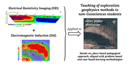
In the past decades, another trend has been the expansion of the use of geophysical methods to areas that are not traditionally included in geosciences. It is the case for agriculture and forestry applications. In the context of a collaboration with the Department of Agricultural and Forestry Engineering at the University of Valladolid, Spain, a module on geophysical methods applied to a forest context was taught within a course on “Forest Soils and Carbon Sequestration” (an optative taught in the second semester of the fourth and final year of the Degree in Forestry Engineering and Natural Environment). Paradoxically (or not so much), besides the aspects peculiar to the forest context, this case turned out to be a good example of the context/limitations abovementioned concerning an exploration geophysics course within a geosciences undergraduate degree (viz limited time and the need to focus on a selected number of geophysical methods, plus its implications from the theoretical approach to the final interpretation stages). The fact that forestry and natural-environment matters and activities also have a very close link with the field and the soil, and therefore students were used to it, facilitated the progress of the learning process.

Within the wider pedagogical panorama, and specifically in the case of geophysical methods, we may find a variety of concerns and approaches that, in general, have in common the recognition of the importance of field education (extensible to geosciences in general). In this context, Waldron et al. [1], addressing the recognized difficulty that students experience in transferring their classroom knowledge to the field environment, describe the building and use of a “geoscience garden”. Related approaches include the construction of an on-campus well field to ease the access to wells with the purpose of, namely, being used for borehole geophysics teaching [2]; and the creation of an “environmental field station” supporting the use of seismic, Ground Penetrating Radar (GPR), magnetic, and electrical resistivity methods for teaching purposes [3]. As for the methodological approaches, May and Gibbons [4] support the view that undergraduate geoscience programs can be enhanced with relatively small additions, such as short courses taught in the field, on the occasion of an environment-oriented four-day course on geophysical methods; this is in line with an equipment-intensive field methods course in Environmental geoscience proposed by Tibbs and Cwick [5] that involved the learning of the GPR system. Field analogs have also been proposed as a learning tool, such as the tabletop models for electrical and electromagnetic (EM) methods developed by Young [6].

Conceptual trends in methodological approaches are diverse. With published examples within the geosciences, they include, for example, service-learning projects, such as a case within upper-division Earth sciences courses reported by Liu et al. [7], in which GPR, EM, and DC resistivity (and other methods) were taught in a practical way. Problem-based learning (PBL) is another pedagogical approach, with roots in medical schools, that has seen growing application within that knowledge area. Some examples exist in the Earth sciences field, such as those presented by Pinto et al. [8] in a geology and environment context, and by Occhipinti [9]; nevertheless, its use within Earth sciences seems to remain subdued.

The module here concerned, focused on geophysical methods applied to a forest context, took place, for a considerable part, on a case-based learning (CBL) basis. Closely related to PBL, the CBL approach was considered to have the potential to fit with our module’s frame; with its well-defined departing point, the module had a mixed self-constructed guided nature, while integrating the abovementioned fieldwork concerns and targeting similar objectives.

Geosciences (geology in particular) are frequently viewed as less exact, rigorous, and objective than subjects such as physics or chemistry, for example. A discussion on this matter is undertaken in a review by King [10], including the views of Baker [11], Bezzi [12], Frodeman [13], and Orion and Ault [14]. In the same line of thought, it stands out the conceptual and effective difficulty of handling a complex system (the Earth, or parts of it) where the researcher is forced to deal with uncertainty and incomplete data. The geophysical approach has the rigorous side of the methods employed and the measurements obtained while having to deal with the issues just mentioned when it comes to incomplete data, the non-uniqueness of geophysical data interpretation, and the transposition stage to the geological interpretation. Owing to this particular situation, geophysical methods may stand in a good position to put students in contact with the uncertainty side of geosciences, particularly through a concrete situation such as the case-based module here concerned. Moreover, it provides a very good frame for a group dynamics approach, from the stage of data acquisition up to the stages of data processing, analysis, and interpretation, while targeting the development of skills at the level of potentialities/limitations evaluation on data acquisition and the methods used, on data quality, and on data interpretation and uncertainty sources, thus supporting the development of critical thinking and the dimension of teamwork.

2. Description of the Learning Activity—The First Stages

The overall approach considers an initial introductory lecture to the methods to be used, their main underlying principles, and the associated specific terminology, while taking into account the following steps, namely the field situation and the survey execution (“Indoors 1”, below). From this point onward, the approach had essentially a self-constructed guided nature, with occasional short lecture-type interventions on topics needing to be elucidated.

Fieldwork was carried out in two stages, with an intermediate data analysis stage in between, as described below. Following the survey execution, the main steps included the processing, analysis, and geophysical interpretation of data; the transposition to the geological context (geological interpretation); and addressing the link with the forest context and the broader implications, such as possible environmental issues.

Groups were formed based on four elements, with the possibility of joining groups or splitting groups for specific tasks.

2.1. Indoors 1

• Time span: 4 h.

The case is presented to the students. The choice of the geophysical methods is discussed, followed by a brief theoretical introduction to the chosen methods.

• The choice of the methods: In the present case, students knew about methods such as the GPR and EM-38 but had no previous knowledge of geophysical methods in a structured way. In geology courses, students may have already followed a course on geophysics of the Earth. It is then possible to discuss the choice of the methods with increased participation of the students. In this case, it had to be guided to a greater degree.
• The theoretical introduction: The main points are summarized in Section 2.1.3 and Section 2.1.4. It is oriented by taking into account the subsequent tasks to be executed.

2.1.1. The Case: The Plot, the Terrain, and the Forest

The plot is close to Soto de Cerrato, 8 km SE of Palencia, Spain (Figure 1). The terrain, overall flat, with very slight altitude variations, borders the Pisuerga River, and is constituted by alluvial deposits of this river. Lateral variations in the sediment composition of these deposits are related, namely, to the presence of old meanders of the river [15]; and, in their turn, they are at the origin of lateral variations in the soils which are partially visible by surface observation. In this plot, a silver poplar (Populus alba L.) plantation, with trees arranged in a 6×6 m grid (i.e., 6 m apart from each other in both NS and EW directions), shows some variability in what concerns tree growth.

In the survey area, the maximum height above a nearby pond is approximately 2–2.5 m. This pond is located 10 m far from the northeasternmost trees of the plantation.

The starting hypothesis: Tree growth variability is related to soil variability (from a geological viewpoint, as shall be seen, soil variability and sediment variability are very much interconnected).

2.1.2. Choosing the Geophysical Methods

The context is that of near-surface geophysics (very near-surface). It is pointed out that a wide range of geophysical methods may be potentially used. Therefore, some criteria must be used in making a choice. The first criterion is to have a contrast in the relevant physical property/the measured parameter(s) (in a first approach, equipment availability is not taken into account); it is underlined that, in some methods (e.g., gravitational methods), the relevant physical property and the measured parameter(s) may not be the same. In a second step, penetration/investigation depth is taken into account: the method(s) to be used must have a shallow penetration depth. In a third step, the speed/cost of acquisition is introduced as a criterion.

Relevant information concerns the fact that geophysical methods have been used for decades in agriculture applications, and, although less used in forestry, a growing number of studies show the potential of these methods in forest contexts, as well (as is exemplified in Section 3.1). This is particularly the case for electrical resistivity and electromagnetic induction methods, to which we should add GPR, precisely because these methods fulfill the above criteria. Among electrical resistivity methods, the one that has been mainly used is Electrical Resistivity Imaging (ERI, also designated as electrical resistivity tomography), while in what concerns electromagnetic induction methods, a number of studies have been conducted with EM-31/EM-38-type instruments.

EM-38-type instruments have been widely used in agriculture contexts for their very shallow penetration depth. In forest contexts, the soil depth of interest is higher, and, for that reason, the EM-31, with a penetration depth in the range of 3–6 m, was used in the present case. Most commonly, in forest studies, either a single geophysical method is used or a joint usage of ERI or EM-31/38 with GPR is the case. Here, at Soto de Cerrato, a joint usage of EM-31 and ERI was the choice, which constitutes a convenient example of how one method potentiates the other. The EM-31 allows for quick acquisition and the elaboration of a map, and, on the basis of this map, the location for ERI profiles is defined. ERI delivers a detailed 2D image of the terrain.

2.1.3. On the Electrical Resistivity Methods and the Instrument

In the electrical resistivity methods, for practical purposes, the relevant physical property and the measured parameter are the same, precisely the electrical resistivity of the terrain. To understand what we actually measure and the fundamental difference between electrical resistivity and apparent electrical resistivity, some development is needed.

The starting situation is that of a homogeneous and isotropic terrain. Here, the fundamental relation is that for the electrical potential, V, created by a point-source of current, I, located on the surface of a terrain with electrical resistivity, ρ, on a point, M, at a distance, r, V = (Iρ)/(2πr). From this relation, it is straightforward to derive the resultant potential V created by a positive current electrode (A⁺ or C₁⁺) and a negative current electrode (B⁻ or C₂⁻) on a point, M, at distances r₁ and r₂, respectively. Considering a random disposition of 4 electrodes on the surface of the terrain—2 current electrodes, A⁺ and B⁻; and 2 potential electrodes, M or P₁ stuck into the terrain at point M, and N or P₂ stuck at a point N—we have for the potential difference between points M and N:

$${\mathsf{\Delta }\mathrm{V}}_{\mathrm{MN}}=\frac{\mathrm{I}\mathsf{\rho }}{2\mathsf{\pi }}\left(\frac{1}{\overline{\mathrm{AM}}}-\frac{1}{\overline{\mathrm{BM}}}-\frac{1}{\overline{\mathrm{AN}}}+\frac{1}{\overline{\mathrm{BN}}}\right).$$

(1)

From this, we may derive the expression for the electrical resistivity for any configuration of the four electrodes. In general, in specific arrays, some type of symmetry in the configuration of the electrodes is sought. In the dipole–dipole array, the four electrodes are inline, with a pair of current electrodes (A and B) on one side and a pair of potential electrodes (M and N) on the other side; and with an equal distance, a, between A and B and between M and N, and a distance (na) between the inner electrodes (B–M). For the dipole–dipole we have, for the electrical resistivity: ρ = K(ΔV_MN/I), with K = πn(n + 1)(n + 2)a. K is the geometrical factor and depends only on the configuration of the four electrodes and the distances between them. What is actually measured is the potential difference, ΔV_MN, between the M and N electrodes and the current intensity, I, between the A and B electrodes; however, from these and the geometrical factor (K), the electrical resistivity (ρ) of the homogeneous and isotropic terrain is readily obtained (such a theoretical approach may be found in [16,17]).

Real terrains are almost always inhomogeneous; in this case, from K, ΔV_MN, and I, we no longer obtain the resistivity (ρ) of the terrain but a value that reflects the influence of multiple domains in the terrain, each with its resistivity, ρ₁, ρ₂, etc.; we thus talk about an apparent resistivity, ρ_a, and we write ρ_a = K(ΔV_MN/I).

In the basis of the ERI technique (and of every point-electrode electrical resistivity method) is a 4-electrode array, as previously described; in the present case, the specific array used in the measurements was a dipole–dipole. In this technique, a greater number of electrodes (greater than 4) are stuck into the terrain, at an equal spacing, prior to any measurements—they may amount from a few to several tens of electrodes. Then a resistivity meter undertakes a measurement sequence, automatically switching from a 4-electrode group to the next one. Starting with the minimum possible distance between the electrodes (for a dipole–dipole, with the distance (a) being equal to the spacing between two consecutive electrodes, and n = 1), a first electrical resistivity profile is obtained with the shallowest investigation depth. Increasing the spacing between electrodes (just by making n = 2), a second resistivity profile is obtained with a higher investigation depth. Continuing this procedure of increasing the spacing between electrodes at each consecutive profile, an apparent resistivity 2D section is thus obtained. The fact that by increasing the spacing between the electrodes the investigation depth also increases is linked to the fact that the electrical current between the electrodes A⁺ and B⁻ flows in volume, thus penetrating into the terrain. It should be noted that, from a methodological viewpoint, it is more convenient to introduce this subject with a Schlumberger or a Wenner array, which actually happened, but we omit it so as to not overburden the text.

ERI measurements were carried out with an Iris Instruments (Orléans, France) Syscal Jr. resistivity meter with a Switch device; the system operates with 48 electrodes in a single measurement sequence.

2.1.4. On the EM-31—The Method and the Instrument

The EM-31 (Geonics, Mississauga, ON, Canada) is an electromagnetic induction instrument with a transmitter coil and a receiver coil kept at a constant distance (3.66 m), usually operated ~1 m above the ground; the operating frequency is 9.8 kHz. The instrument measures the terrain’s apparent electrical conductivity. The transmitter coil, energized with an alternating current, produces an electromagnetic field (primary field), which induces very small currents in the terrain. These currents, in turn, generate a secondary field. The receiver coil senses both the primary and secondary fields. In the operating conditions of the EM-31, in a homogeneous half-space, the ratio of the secondary to the primary magnetic field components is linearly proportional to the electrical conductivity of the terrain. The instrument actually measures this ratio. In a layered terrain, the contribution of each layer to the measured apparent conductivity depends on its depth, its thickness, and its conductivity [18].

Two operating modes are possible: the “normal” position corresponds to the vertical dipole mode (Vd-mode), in which the plane of the coils is horizontal; rotating the instrument 90° on its side, measurements are performed in the horizontal dipole mode (Hd-mode), in which the plane of the coils is vertical. In the vertical dipole mode, the penetration depth is ~6 m, while in the horizontal dipole mode, it is ~3 m.

2.2. In the Field 1 (Measuring with the EM-31 + Tree Diameter)

• Time span: half-day ×2. Students undertook fieldwork in two groups of eight (two turns)—one in the morning and the second in the afternoon.
• Equipment: 1 EM-31 + 2 tree calipers + 3 GPS receivers + 1 tape measure
• Outcomes: 1 set of apparent conductivity measurements + 1 set (partial) of tree diameter measurements; at the end of this phase, the EM-31 survey was accomplished, and tree measurements were partially performed.

In all stages in the field, students undertook fieldwork in groups, rotating between the different tasks to be performed.

• Description:

This first phase consisted of the EM-31 survey and the measurement of tree diameters. In the limit, EM-31 measurements may be carried out by just one person; a crew of two is preferable. In this activity, four students at a time (one group) rotated between measuring with the EM-31, taking UTM coordinates, and marking the following measurement point. At the same time, the four remaining students, split into groups of two, undertook tree diameter measurements.

Measurements with the EM-31. The EM-31 is an instrument that allows for a quick survey of the terrain. EM-31 profiles were carried out along the midline of tree rows at 10 m spacing. At each measuring point, apparent conductivity readings were taken in the two modes (Vd-mode and Hd-mode); additionally, GPS UTM coordinates (northing and easting) were also taken. The overall survey consisted of a set of parallel lines executed in two perpendicular directions: EW profiles spaced 18 m and NS profiles spaced 42 m.

Tree size/diameter measurements. The tree diameter was measured at 1.3 m above the ground: two values at right angles were read and the mean value was taken as the diameter.

2.3. Indoors 2 (Preliminary EM-31 Data Analysis and Interpretation)

• Time span: 2 h.
• Starting point: 1 set of EM-31 apparent conductivity measurements.
• Software used: Excel and ArcGis.
• Relevant information provided/remembered: the geological context (plus the geological map); tables (different authors) of the electrical resistivities of different rock types; penetration depth values for the Hd-mode and the Vd-mode.
• Outcomes (1): 1 set of apparent resistivity values converted from apparent conductivity measurements; 2 apparent resistivity maps (Hd-mode and Vd-mode).
• Outcomes (2): first EM-31 data analysis and interpretation results; new hypotheses; the position of 3 ERI profiles.

Firstly, groups worked on data to produce outcomes (1). In a second moment, groups analyzed and discussed outcomes (1), using the information provided/remembered. A final discussion involved all the groups and the instructor; the “Description/Discussion” below reflects such an analysis and discussion with the groups. This approach was replicated in subsequent stages.

• Description/Discussion:

Geophysical data processing involves some form of field data handling which may or may not include data inversion/modeling; almost always, it should come to a graphical representation. In data analysis and interpretation, two stages are usually present: a first stage at the geophysical level and a second stage where the transition to the geological/other level is sought.

EM-31 data were organized (converted from apparent conductivity to apparent resistivity), gridded by using a kriging method, and then plotted. A contour map of the surveyed area was created for each measuring mode, and, from these maps, the locations to execute the ERI profiles were chosen.

As stated above, the EM-31 reads the apparent electrical conductivity of the terrain, with output values in mS/m; however, as ERI values (to be obtained) correspond to apparent resistivities, the choice was made to convert the EM-31 apparent conductivities to apparent resistivity values in Ω·m (by performing “value (Ω·m) = 1000/value (mS/m)”). The resulting maps are shown in Figure 2: the apparent resistivity map for the Vd-mode is in Figure 2a, and for the Hd-mode, it is in Figure 2b.

In both figures, the striking feature is the curved higher apparent resistivity area with low apparent resistivity areas on both sides. For the interpretation of such feature, two pieces of information are pertinent: the geological context—we are in alluvial deposits of the Pisuerga; and the general relationship between sediment grain size and the electrical resistivity—there is a general tendency for non-consolidated coarse-grained sediments to show higher electrical resistivities than fine-grained ones, with rich-clay layers usually showing low to very low resistivities [19,20,21]. The shape of this feature raises the hypothesis that it may correspond to an old meander of the Pisuerga River. The contrast in apparent resistivity values between this paleochannel and the side areas would be directly related to sediment grain size or, otherwise, to the soil texture: the coarse grains’ fraction in the soil would be significantly higher in the higher apparent resistivity meander area than in the low apparent resistivity side areas—a second interrelated hypothesis to be verified.

For corresponding areas, the apparent resistivity values are lower in Figure 2a relative to Figure 2b. Knowing that the penetration depth for the Vd-mode (~6 m) is higher than for the Hd-mode (~3 m), in a first approach, this suggests that, for the whole area in general, the resistivity of the terrain at higher depths should be lower than in the upper soil levels (this is discussed in further detail in Section 4.2).

Based on these maps and following the above discussion on the possible significance of higher/lower apparent resistivity areas and their composition, three ERI profiles were placed across a two-zone limit, approximately at a right angle to this limit, in the central part of the survey area, along the midlines of approximately NS tree rows, at a convenient distance between each other, as shown in Figure 2b. Additionally, it was decided to collect soil samples associated with these profiles.

2.4. In the Field 2 (ERI Profiles + Soil Sampling + Finishing Tree Measurements)

• Time span: 1 day ×2. Students undertook fieldwork in two groups of eight (two turns); one group per day.
• Equipment: 1 Syscal Jr. resistivity meter with a Switch device + auxiliary equipment (cables, electrodes, etc.) + 1 tree caliper + 2 earth augers + 2 GPS receivers + 2 tape measures.
• Outcomes: 3 dipole–dipole ERI profiles; 1 set (partial) of tree diameter measurements; 20 × 2 soil samples.

• Description:

Initially, the 8 students were engaged in positioning and deploying all the equipment required to undertake the ERI measurements. After a long enough section of the first profile was acquired, it was used to place the first soil sampling points. Soil samples were collected by a group of 2 students. Another group of 2 students continued tree diameter measurements (all tasks on a rotating basis).

ERI profiles. Fieldwork related to ERI profiles included several tasks. It started with placing the profile, in this case along the midline of two tree rows; a 50 m tape measure was deployed along the ground surface; 48 electrodes were stuck into the terrain at 0.5 m spacing, corresponding to a first profile segment of 23.5 m; and they were then connected to a multi-conductor cable, which in turn was connected to the resistivity meter + switch device. A rolling approach to increase the profile length (12 m per additional segment), which uses an extra cable, was adopted: the total length of Profiles 1 and 3 was 47.5 m, and it was 59.5 m for Profile 2. Proper electrode connection and circuit resistance between consecutive pairs of electrodes were checked. Measurements were undertaken according to a sequence previously uploaded to the resistivity meter using the dipole–dipole array.

Soil sampling. An initial quick processing of ERI data delivered usable (but non-final) resistivity sections; the choice of the points along each profile of where to collect samples was guided by resistivity values in those sections. Samples were collected in the 0–30 cm and 30–60 cm range depths.

Finishing the tree diameter measurements. Meanwhile, tree diameter measurements were finished.

2.5. Indoors 3

• Time span: 6 h.
• Final data processing, analysis, and interpretation take place. Results are discussed.

2.5.1. Joint EM-31 + Tree Diameter Data Analysis and Interpretation

• Starting point: 1 set of EM-31 apparent resistivity values; 2 apparent resistivity maps (Hd-mode and Vd-mode), both from Section 2.3; and 1 set (complete) of tree diameter measurements.
• Software used: Excel; ArcGis.
• Relevant data provided: map of visible cobble+pebbles zone in the survey area; apparent resistivity values at tree location obtained by kriging of the original values.
• Outcomes (1): superposed maps of EM-31 apparent resistivities and tree diameters; plot of tree diameter–Hd-mode apparent resistivity.
• Outcomes (2): correlation of the 2 sets of data (apparent resistivities and tree diameter); subdivision of the survey area into zones; simple statistical results.
• Outcomes (3): data analysis confirms the existence of a correlation between the EM-31 values and the diameter of the trees.

Initially, the groups worked on the material abovementioned in “starting point”. Following the analysis and discussion of results, data mentioned as “relevant data provided” were introduced.

• Description/Discussion:

The tree measurement data were integrated with the EM-31 data. In Figure 3, the distribution of the trees’ diameter was superposed on one of the precedent figures (Figure 2b); as the maps in Figure 2a,b show the same basic spatial pattern, only the Hd-mode apparent resistivity map, corresponding to a shallower penetration depth, was used in this step (further details are addressed in Section 4.2.1). Using the maps in Figure 2 as a first criterion and the tree diameter as a second criterion, it was proposed to the students to subdivide the survey area into zones.

The result is shown in Figure 3a. In Figure 2a,b and Figure 3a, the limit of the supposed paleochannel coincides roughly with the 32 Ω·m (Figure 2a) and 56 Ω·m (Figure 2b and Figure 3a) isoresistivity lines, with values ranging from below 20–24 Ω·m to above 40 Ω·m in the Vd-mode, and from below 28–40 Ω·m to above 68 Ω·m in the Hd-mode. There is a strong visual correlation between the size/diameter of the trees and the supposed meander plus the side areas they are associated with, as depicted by the apparent resistivity high/low values. It is most evident that the trees with the larger diameters coincide with the low apparent resistivity side areas, particularly the central one, below 56–40 Ω·m (Zone B), whereas the trees that lie over the supposed paleochannel soils, with higher apparent resistivities, i.e., above 56 Ω·m (Zone A), show consistently smaller diameters.

However, a further analysis of Zone A showed that, particularly in its eastern/northeastern part, some trees with a wider diameter were also present. As the fieldwork with students was terminated, it was decided to map the soil surface, as in part of the terrain pebbles and cobbles were visible on the surface, and to provide this map as an additional piece of information. As a result, Zone A was divided into Subzones A₁ and A₂ (Figure 3b); Subzone A₁ corresponds to the one with a significant amount of pebbles and cobbles visible on the surface. This limit between Subzones A₁ and A₂—and also a limit between Subzone A₁ and Zone B—is superposed in Figure 3b.

Statistical analysis. A simple statistical analysis and joint data plot were proposed. For that purpose, given that trees are spaced 6 m apart, EM-31 values of apparent resistivity at tree location were obtained by kriging of the original values and made available to the students. The correlation coefficients for the pair Hd-mode apparent resistivity–tree diameter show values of −0.70/−0.77 for the whole area and −0.83 for the A₁ + B areas alone (−0.77 and −0.83, excluding trees in the transition area and the 5% most extreme cases); these values are in line with the visual perception in Figure 3. In fact, Figure 4 depicts the situation even better than the correlation coefficients alone: plotting the tree diameter versus the Hd-mode apparent resistivity for all the trees, the observed distribution is stretched but continuous (Figure 4a); however, if we consider only Subzone A₁ and Zone B in the conditions of Figure 4b, we obtain two very distinct populations, with distinct tree diameters and Hd-mode apparent resistivity limits.

Therefore, the existence of a correlation between the EM-31 values and the diameter of the trees, particularly in what concerns Subzone A₁ and Zone B, is an important point that the above analysis allows us to establish.

2.5.2. ERI Profiles and Soil Sampling Results—Discussion

• Starting point: 3 apparent resistivity sections’ data; soil samples.
• Software used: RES2Dinv and Excel.
• Task (1): RES2Dinv main features “exploration”; soil sample simple granulometric analyses.
• Task (2): processing the 3 apparent resistivity sections’ data; calculus of the saturation degree by using Archie’s equation.
• Task (3): integrated data analysis (geophysical level plus transition to soil/geological level). Starts with groupwork outside the classroom; final discussion with the instructor.
• Relevant theoretical framework: Archie’s equation and its frame are introduced (this subject is treated in more detail in Section 3).
• Outcomes (1): 3 processed resistivity sections; soil sample results; soil saturation estimates in Zone A.
• Outcomes (2): vertical characterization of the terrain to the depth of the resistivity sections.

• Description/Discussion:

Obtaining the resistivity section. Students processed ERI data with RES2Dinv software (Geotomo Software SDN BHD, Penang, Malaysia), for which a semi-open version is available. The basic output of processed data for Profile 1 (P1) is shown in Figure 5. In this figure, the upper section corresponds to the contoured apparent resistivity values measured in the field. The bottom section is obtained by inversion of the field apparent resistivity data in an iterative process [22]; in this bottom section, we have a model of the “real” resistivity distribution in the terrain. The middle section corresponds to the apparent resistivity values generated in each iteration from the resistivity distribution in the bottom section; this middle section is compared with the upper section, thus resulting in the absolute error value indicated. In each iteration, the bottom section is adjusted in order to minimize that misfit value.

The groups went through data quality evaluation, namely on the basis of the resistance value between consecutive pairs of electrodes; the repeated measurements obtained in the rolling process; the electrical resistivity evolution along each level in the apparent resistivity section (specific RES2Dinv function); and the above-mentioned final misfit value. The groups explored the main features of RES2Dinv and could verify a major characteristic of geophysical data modeling–the non-uniqueness of such models. Specific to data processing with RES2Dinv (and similar software) is the fact that the iteration with the lowest “error” value may not be the one corresponding to the “best model”. In line with what is stated in the software’s manual [22], the best result often corresponds to the iteration after which the “error” does not change significantly; continuing the process frequently leads to the creation of artifacts.

Soil sampling results. As stated in Section 2.4, soil samples were collected along the three profiles at selected points in the 0–30 cm and 30–60 cm range depths. The students conducted a simple granulometric analysis that consisted of separating fractions above and below 2 mm, weighing the initial sample and the two separated fractions, and determining the percentage of each one. The results are shown in

Table 1. Coarse grain fraction percentage in soil samples (>2 mm). Distances from the beginning of each ERI profile.

Profile 1
Distance (m)		5.50	11.25	20.50	23.50	24.50	27.5	33.00	35.50	39.75
Depth range (cm)	0–30	66.9	63.6	58.4	14.1	16.2	14.4	35.4	37.4	30.3
	30–60	72.6	76.6	39.9	9.6	16.2	18.4	31.6	31.7	39.1
Profile 2
Distance (m)		12.50	15.00	26.50	34.00	36.50	44.50
Depth range (cm)	0–30	72.4	65.3	16.2	29.8	18.1	3.1
	30–60	79.0	70.9	61.0	26.0	33.5	(7.2) *
Profile 3
Distance (m)		11.00	15.25	26.50	32.00	38.75
Depth range (cm)	0–30	61.8	74.5	1.0	8.4	6.4
	30–60	72.2	75.3	1.1	2.1	4.0

* Depth fell short of 60 cm.

.

The three ERI profiles. Processing the three ERI profiles with topography delivered the resistivity sections shown in Figure 6 (which are equivalent to the bottom one in Figure 5). In these resistivity sections, the reference level for the elevation scale corresponds to the water surface in the nearby northeastern pond. In the following discussion, an “early assumption” is made that the water level in the survey area, particularly in Zone A, is essentially the same as in the nearby pond (based on its proximity to the pond plus the coarse nature of the sediments, to be discussed below, and therefore the very high soil permeability; and the low level of the area, which is occasionally flooded by the rising waters of the Pisuerga). In all three resistivity sections, a major difference between Zones A (to the north) and B (to the south) is most evident.

• Profile 1—Figure 6a

In the southern half of P1 (Zone B), a surface soil layer, ~0.8 m thick, shows resistivities in the 70−300 Ω·m range, locally lower. Below a depth of ~0.8 m, resistivities are low, close to 15–20 Ω·m; these low values are usually indicative of the presence of a significant clay fraction in the soil. In the northern half (Zone A), high resistivities, reaching values over 1600 Ω·m, are present at depths ~0.5–1.7 m; in the upper 0.5 m, resistivities are somewhat lower, starting at ~400 Ω·m (in the first 17.5 m of the section).

In this upper part of the soil, resistivity differences between the northern and the southern sides are linked to soil differences, as expressed by the coarse fraction (>2 mm) in the soil; the values for 0−30 cm and 30−60 cm are shown in Table 1: over 63%/700 Ω·m at 5.5 m and 11.25 m; 30−40%/100−300 Ω·m after 33.0 m; and 10–20%/<100–150 Ω·m in the central part between 23.5 and 27.5 m. Values at 23.5 and 24.5 m and the intermediate values at 20.5 m are important for understanding tree growth differences in the transition area between Zones A and B (17.5–23.5 m); this is discussed in Section 4.3.4.

Resistivity values of 1600 Ω·m and over, at depths ~0.5−1.7 m, in the northern half of the section, can be explained by the very nature of the soil constitution. Based on soil samples (particularly in the 30−60 cm range) and the resistivities present in the section in Figure 6a (0–0.5 m; ~0.5–1.7 m), it is very likely that the soil constitution in the ~0.5−1.7 m range is much the same as in the first 0.6 m of the terrain—a “late assumption”/conclusion reinforced by the following discussion. The very high percentage of the coarse fraction makes it the equivalent of a non-consolidated conglomerate in geological terms; the usual resistivity values for this fully water-saturated rock type are in the 150−500 Ω·m range [19]. A soil/rock with such a high coarse fraction percentage has a low water retention capability, and even though the water table is most likely at a shallow depth, the saturation degree may be significantly below full saturation. For the above 150−500 Ω·m saturated case and for a resistivity value of 1600 Ω·m, Archie’s equation in Section 3.2 points to a saturation degree in the 56−30% range. In the northern part of the section, the resistivity transition, near the 0 m elevation, from values of 800−1600+ Ω·m to values in the 100−300 Ω·m range is compatible with the full saturation of the soil (reaching the water table); additionally, a change in the soil composition cannot be excluded.

• Profiles 2 and 3—Figure 6b,c

The resistivity sections in Figure 6b (P2) and Figure 6c (P3) show the same main features described above for Figure 6a (P1). Differences are present mainly in the southern half (Zone B) “upper layer”: compared to Section 1 (Figure 6a), the upper 1.0 m in Section 2 (Figure 6b) is more differentiated, with a thin low resistivity first layer (with a corresponding lower coarse fraction percentage in the 0−30 cm interval at 36.5 and 44.5 m distances), followed by a 250−600 Ω·m second layer. In Section 3 (Figure 6c), this “upper layer” shows an overall lower resistivity than in Section 1 and Section 2, with values under 100 Ω·m for the entire 0.7−1.0 m thickness; this is in correspondence with the low/very low coarse fraction percentage both in the 0−30 and 30−60 cm intervals, at distances 32.0 and 38.75 m. Therefore, in addition to the main difference between Zone A and Zone B, lateral variability is also present in this “upper layer” of Zone B.

3. Enlarging the Context and Gaining Insight into Archie’s Equation Implications

• Time span (Section 3 and Section 4): 6 h + groupwork outside classroom.
• Starting point: bibliography on studies in forest contexts with the use of geophysical methods (groups encouraged to look for more).
• Task (1): Analysis of cases in the bibliography (guidelines: focus on the situation/the problem, the geophysical methods involved, and the connection with Archie’s equation).
• Task (2): Exploration of Archie’s equation implications.

Until now, the EM-31 survey plus the ERI profiles, together with soil samples information and the tree measurements, allowed us to create a “3D image” of the soil constitution and variability in the upper meters of the terrain and of its relationship with tree variability throughout the silver poplar plantation area. It is time to briefly look at the type of problems a number of researchers have come across in a forest context in which geophysical methods have been used and to put the present case into perspective relative to those studies, particularly in regard to what concerns Archie’s equation implications.

3.1. Overview of Previous Studies in Forest Contexts Based on Geophysical Methods

In forest contexts, geophysical methods have been primarily used to assess soil water content availability and variability, both spatially and temporally. It is the case for the use of ERI to measure soil moisture availability and plant water use in a Mediterranean natural area [23], to assess seasonal/temporal change and spatial variability in soil water content in a temperate-climate deciduous forest [24] and a Scots pine forest + shrub environment in Scotland [25], or to evaluate the relationship between soil water storage capacity and silver fir vulnerability to drought-induced soil water deficits in a Mediterranean area [26]; variations in tree responses to drought were also put in relation with the spatial variability in total available water content estimated from ERI measurements [27].

As for electromagnetic induction methods, they have proven their potentialities in soil salinity measurements, as is the case for the use of the EM-38 in eucalyptus plantations in Australia, both to evaluate the impact of the salinity level on the survival and growth rate of trees and to guide future plantations [28]; in a similar environment, the EM-38′s “cousin”, the EM-31, with a higher penetration depth, has also been used for soil salinity evaluation purposes [29].

Other applications include the use of the EM-31 for the study of soil erosion in a forested area [30], and of ERI in the evaluation of tree root systems’ impact on the soil and regolith profile [31], as well as the use of a shallow investigation depth fixed-length electrical resistivity array for forest soil-property-monitoring purposes [32].

In some situations, the ERI method has been used together with GPR. It is the case in a study on water and root distribution in shallow soils [33].

In the vast majority of situations, such as those mentioned above, where ERI and EM-31/38-type instruments are used in forest contexts, even if the terrain/soil matrix is implicitly taken into account, the focus is either on the soil water content or the soil salinity; that is to say that, if we consider Archie’s equation, the main interest lies in the water saturation degree (S_w) or the pore-filling water resistivity (ρ_w), not on the formation factor (F), as is discussed below. At Soto de Cerrato, the focus is on the sediment/soil itself, its variations, and its relationship to tree growth variability within a monoculture silver poplar plantation.

3.2. The Situation in Soto de Cerrato and Archie’s Equation

Archie’s equation is mentioned in the literature in relation to electrical resistivity/conductivity measurements on several occasions (in [23,25,33,34], for instance). As a matter of fact, in a number of these situations in the literature, it is used mainly for its conceptual utility, with the parameters involved not being quantitatively determined; it is also predominantly the case here.

Archie’s equation was established on an empirical basis in geological contexts [35], and in an evolved form from the original one, it may read ρ_r = ρ_w.aϕ^−m.S_w⁻ⁿ (as written, for instance, in [36]), with ρ_r being the electrical resistivity of the rock/soil, ρ_w the electrical resistivity of the pore filling water, ϕ the porosity of the rock/soil, a and m parameters that depend on the lithology/soil, S_w the water saturation degree of the rock/soil, and n a parameter that usually has a value ≈ 2 (even though it may be higher when S_w < 30%; [16]). In this equation, F = aϕ^−m (the formation factor) depends only on the characteristics of the rock/soil matrix. When Archie’s equation is applied to agricultural contexts with soils that are regularly subject to cycles of tilling and compaction, the F does change with time. However, in forest contexts, the soil depth of interest is usually significantly higher than in agricultural ones, and, after an eventual initial localized impact of plantation works on the upper soil levels, the terrain is temporally stable.

In soil salinity studies, the critical parameter is ρ_w, which decreases with increasing salinity of the soil/pore-filling water. When the soil water content is the main concern, particularly when the interest is in soil water availability over time and on the impact of drought periods, S_w is the main parameter we are looking at. These issues are discussed further below in what concerns Soto de Cerrato. For the moment, it is stressed that, in the plot area, the water table level is most probably at shallow depths, as previously mentioned, thus significantly reducing the concerns with water availability.

Here, at Soto de Cerrato, our attention is focused on terrain variability (sediment/soil variability), which has a primary impact on the formation factor, F, with this being the underlying cause of sediment/soil electrical resistivity (ρ_r) variations; and this, in turn, reflects on the spatial changes in the apparent conductivity/resistivity, as measured with EM-31 and ERI techniques.

Particularly in what concerns the upper soil levels, it is also expectable that some variability in the saturation degree, S_w, contributes to changes in ρ_r and, thus, to differences in apparent conductivity/resistivity measurements. However, at Soto de Cerrato, S_w is sediment/soil-dependent, so, in the end, it is still the spatial differences in the sediment/soil characteristics that account for the variation in apparent conductivity/resistivity measurements.

Finally, we must bear in mind that Archie’s equation has reduced applicability when the clay content is high; in such a case, as a rule, the presence of clay has the effect of increasing the terrain’s apparent conductivity (lowering the apparent resistivity), as measured by EM-31 and ERI instruments.

4. Overall Discussion

Recovering an initial statement, working within the geosciences field implies dealing with uncertainty and incomplete data to a greater or lesser degree, depending on the situations. It should be part of a course in geophysical methods both to make students aware of this fact and to be capable of handling it, which also means developing some criticism at each phase, from choosing the method(s) to be used up to the interpretation stage.

4.1. Potentialities and Limitations of the Chosen Methods and the Importance of Their Combined Use

Each geophysical method has potentialities and limitations. Measuring with the EM-31 is rather fast, which allowed for creating a map in a short time. However, even though measuring in two modes (Hd and Vd) may give indications of the vertical evolution of the terrain/soil, it lacks 2D vertical imaging capabilities. For the soil depth of interest in the present case, the EM-31 is a well-suited system, but it may lack penetration depth for studies requiring depths greater than ~6 m to be investigated; otherwise, it is too high if we are interested just in the upper soil 0.5−1.0 m. Compared to the EM-31, the ERI method is more “heavy”; that is, it requires more equipment, is more time-consuming, and requires a larger field team, but it has 2D (and even 3D) capabilities. Moreover, up to a certain point, the investigation depth of ERI is adjustable by varying the basic inter-electrode spacing. Combining the EM induction and ERI methods allowed us to bring together the speed and mapping capabilities of the EM-31 and the 2D imaging possibilities of the ERI.

4.2. Data, Concepts, and Models

4.2.1. On Data Evaluation and the EM-31 Penetration Depth

A critical view should also be present in what concerns data quality (in a broad sense). EM-31 apparent resistivity values look coherent with 2D apparent resistivity and inverted resistivity ERI values in Zone B; however, in Zone A, at first sight, it is possible that one would expect higher EM-31 apparent resistivity values, particularly for the Hd-mode, for which the penetration depth is ~3 m. This brings us to a discussion on the reach of the concept of the penetration depth: on one hand, it can be defined on a mathematical ground, and, as such, we may obtain a specific value for this depth; on the other hand, the statement that the Hd-mode penetration depth is ~3 m does not mean that all the signal contribution to the measured apparent conductivity comes entirely from the upper 3 m of the terrain. For the Hd-mode and a specific depth of 3 m, using the equations in [18], for practical purposes, the measured apparent conductivity results from applying a multiplication factor of 0.72 to the electrical conductivity of the upper 3 m and 0.28 to the conductivity of all the terrain below 3 m; using a simple two-layer case, the point is that, if the conductivity of the first layer is very low compared to the second layer, the latter will be preponderant for the measured apparent conductivity.

The situation in Zone A is close to the two-layer case described above. Using a three-layer model with approximate values to the ERI profiles in Figure 6 (depth values indicated ahead)—0.5 m/800 Ω·m (1.25 mS/m), 1.8 m/2400 Ω·m (0.417 mS/m), and 30 Ω·m (33.3 mS/m)—we see that the resulting apparent resistivity values are 69 Ω·m (Hd-mode) and 42 Ω·m (Vd-mode), which are coherent with the values on the maps in Figure 2 and Figure 3. These values (69 and 42 Ω·m) also shed light on another matter: since the penetration depth for the Hd-mode (~3 m) is lower than for the Vd-mode (~6 m), the 69/42 Ω·m values could be envisaged as the Vd-mode “reaching” a low resistivity layer at a depth that no longer has a significant influence on the Hd-mode. This was the first approach (Section 2.3), and we cannot exclude that possibility, but the above three-layer model is enough to set the possibility of the 69/42 Ω·m values, and this, in turn, is an example of the non-uniqueness of geophysical data interpretation.

4.2.2. Further Insight on the Usefulness of Concepts and Models to Help Thinking about a Situation

In the previous paragraph, and talking about the Hd-mode, the penetration depth is ~3 m (read “close to 3 m”), but the investigation depth is probably higher than 3 m. This affirmation may sound strange because, in the last few decades, the terms “penetration depth”, “investigation depth”, and others (such as “exploration depth”) have frequently been used as synonyms. However, in past times, the use of the term “investigation depth” had a somewhat different meaning. A discussion on it exemplifies the usefulness of loosely defined concepts. The penetration depth is mathematically defined, and a precise value can be obtained for it; and, in the case of the EM-31, it is not situation-dependent. The investigation depth is a loosely defined, semi-quantitative, situation-dependent concept, even in the EM-31 case.

The situations in

Table 2. EM-31 Hd-Mode and Vd-Mode model results (obtained with the equations in [18]); see Figure 7.

Pseudo-Homogeneous Half-Space (Resistivities in Ω·m)	h—1st Layer Thickness (m)	Resistivity (Ω·m)		Hd-Mode Apparent Resistivity (Ω·m)	Vd-Mode Apparent Resistivity (Ω·m)
		Layer 1	Layer 2
1600-2400-3600	4	2400	30	132	-
20-30-45	4	30	2400	38	51
20-30-45	6	30	2400	-	42
1600-2400-3600	144	2400	30	1600	-
1600-2400-3600	36	2400	30	800	-

/Figure 7 help clarify its contours. Let us consider a pseudo-homogeneous half-space with a central resistivity value of 2400 Ω·m and 50% ± variations (central in logarithmic terms; 50% on the lower value in the pair); we will thus have variations in the range 1600–3600 Ω·m. In Figure 7a, this half-space is crossed by a vertical fault; on the other side of the fault, we have a two-layer terrain with an upper 4 m/2400 Ω·m layer and a 30 Ω·m half-space. The question is, if we are performing a transect with an EM-31 and we cross the vertical fault, will the change in the terrain be detectable (will the presence of the 30 Ω·m half-space be detectable)? To be detectable, the apparent resistivity we obtain must be outside the 1600–3600 Ω·m range, preferably clearly outside, and in this case—132 Ω·m in the Hd-mode—it is more than clearly outside. That being said, in such a situation, the investigation depth is sufficient to put in evidence the half-space —it is higher than 4 m— even though the penetration depth for the Hd-mode is 3 m. In Figure 7b, the “opposite” situation is represented: the pseudo-homogeneous half-space has a central resistivity of 30 Ω·m (20–45 Ω·m range); the two-layer terrain has an upper 4 m/30 Ω·m layer and a 2400 Ω·m half-space. In this case, the apparent resistivity obtained in the Hd-mode is 38 Ω·m, inside the 20–45 Ω·m range, and therefore the 2400 Ω·m half-space is undetectable; in other words, in this case, the investigation depth is insufficient to detect the half-space: it is lower than 4 m. The term “investigation depth” thus includes the notion of detectability of a layer/a body (or the potential to do it); this notion is present in Poldini [37] and Meyer de Stadelhofen [19], as well as, under other designation, in Orellana [20].

For the Vd-mode, the apparent resistivity obtained for the last two-layer terrain is 51 Ω·m, outside the 20–45 Ω·m range. Thus, we can say that its investigation depth is sufficient to detect the half-space: it is higher than 4 m. Looking at the results for the Hd-mode and the Vd-mode, the former has an investigation depth that is lower than that of the latter. The expression “investigation depth” may thus be used qualitatively to compare different EM-31 operating modes; this is extensible to other methods, for instance in order to compare different arrays in electrical resistivity methods or different array lengths.

Finally, for a two-layer terrain with a 6 m/30 Ω·m first layer + 2400 Ω·m half-space (6 m instead of 4 m), the apparent resistivity for the Vd-mode would be 42 Ω·m, inside the 20–45 Ω·m range. In this case, even though the penetration depth is 6 m, the investigation depth is lower than 6 m. In Table 2, we added the results for the first considered case with a two-layer terrain with a 2400 Ω·m first layer + 30 Ω·m half-space in the following circumstances: an Hd-mode apparent resistivity of 1600 Ω·m (lower limit of the 1600–3600 Ω·m range) corresponds to the first layer having a thickness of 144 m; and even if we consider half of the former value, i.e., 800 Ω·m, which is clearly outside the 1600–3600 Ω·m range, that corresponds to a 36 m thick first layer, or, in other words, to a situation where the investigation depth in the Hd-mode is higher than 36 m.

4.3. Drawing Conclusions in an Incomplete Data and Uncertainty Framework

The discussion in the following subsections derives from questions that arise as a result of all the acquisition, processing, and interpretation work: What conclusions may we draw from the analysis and interpretation of data? Do the data fall somewhat short in some situations? What about our hypotheses? In the end, what further data acquisition could we recommend/propose?

4.3.1. On the Main Conclusions (and Self-Questioning Their Validity)

EM-31 and ERI data, plus soil granulometric analysis and tree diameter measurements, do confirm the starting hypothesis: tree growth variability is effectively related to soil variability. Zones A and B were established on the basis of apparent resistivity data from the EM-31 (with tree diameter as a second criterion); ERI profiles confirm that the vertical evolution of the soil in the upper 2.5 m is effectively different in Zones A and B; the coarse grain fraction percentage in soil samples collected in the 0–30 cm and 30–60 cm ranges show a clear relationship with the resistivities of these soil depths, with coarser soils related with higher resistivity values; and higher/lower tree diameter values are connected with Zones B and A, respectively. From this summary and the discussion in previous sections, we may affirm that, in Zone A, at least in the upper 1.7–2.0 m, the soil is coarse/very coarse, and tree growth is poorer (particularly in Subzone A₁). In Zone B, the upper 0.8–1.0 m shows some variability in the soil coarse fraction percentage, but it is always significantly lower than in Zone A; below a depth of 0.8–1.0 m, a clay-rich layer is present.

The above paragraph is an example of the way we may state a number of conclusions after data analysis in geosciences. The previous sentences are rather categorical, but it is implicit that we are dealing with incomplete data and some degree of uncertainty. How big that uncertainty is depends on our data, the use and the reasoning we are able to achieve with it, and the confidence we have in the application to our specific case of knowledge from other cases, as well as the general accumulated knowledge within the field of geosciences. Hence, it is proposed to give a second look at the above paragraph.

Soil sample granulometric analyses just differentiate a fraction above 2 mm from a second one below. Is it enough? For our purposes, it is sufficient, given that those fractions have a major influence on soil resistivity/characteristics; and that in Zone A, cobbles and pebbles, present in the coarse fraction in a significant amount, were easily observable. Would it be better to have complete granulometric analyses? The answer is yes, and this may integrate a proposal for future work if a deeper study on the area is sought.

Soil sampling reaches a depth of 60 cm; it reveals a high coarse fraction percentage in Zone A. The statement that, in Zone A, this high coarse fraction is present at least up to a depth of 2 m is clearly an extrapolation. What allows us to do it? The ERI apparent resistivity measurements and the inverted resistivity values in the 0–60 cm and 0.6–2.0 m ranges (sections in Figure 5 and Figure 6), the geological context, and the discussion in Section 2.5.2 involving namely the Archie equation (and its extension in Section 3) are the answer. From here, the extrapolation is set on sound bases. Would it be better to have soil samples from deeper levels? The answer is, again, yes, and that could be another proposal for future work.

It is stated that, in Zone B, below a depth of 0.8–1.0 m, a clay-rich layer is present. In this case, we do not even have a soil sample. The starting point to the reasoning is the general knowledge on low/very low resistivity layers and the geological context (alluvium): in an area close to a river’s mouth (with sea influence), they are related in almost all cases either to a clay-rich composition or to groundwater/soil salinity, or both. In the present case, we are far from the sea, and even though we cannot exclude a salinity cause, it is much less probable. Should the low resistivity layer in Zone B be sandy/gravel and a groundwater salinity problem exist, there should be some continuity between Zone B and Zone A, and the layer resistivity in Zone A should be much lower, at least below its middle-depth; however, this is not the case (Figure 6). Saline soil/groundwater has a negative impact on tree growth, but it is precisely in Zone B that tree growth is higher. Hence, existing evidence is against the salinity hypothesis, supporting instead the existence of a clay-rich layer. Here again, a shallow borehole with soil and water sample collecting could be proposed for future work; it would also allow us to precisely determine the water table level.

4.3.2. On Other Hypotheses

The data and the previous discussion do support the hypothesis raised in Section 2.3 that the coarse grains’ fraction in the soil would be significantly higher in the higher apparent resistivity central curved area than in the low apparent resistivity side areas, thus also supporting the interconnected hypothesis that this curved area corresponds to an old meander of the Pisuerga River. ERI profiles, in conjunction with soil sample analysis, were determinant to come to this conclusion, but their extent is limited (Figure 2 and Figure 3). This implies that an extrapolation is being made to the entire area; it is supported (strongly) by the relationship between two sets of geophysical data with a close nature (EM-31 and ERI) and secondarily by the tree size distribution.

4.3.3. On the ERI Profiles—Section Depth and Basic Electrode Spacing

Within the initial purpose of finding a possible relationship between tree growth and soil composition variability, the ERI basic electrode spacing of 0.5 m was chosen to obtain a high detail in the upper 2.5 m of the terrain, and, for this purpose, it worked well. However, the data analysis shows that for a more complete “image” of the terrain, information from higher depths would be desirable. From the three ERI sections, it is possible to see that some change occurs at a depth of ~2 m in both zones, but there is a lack of information at higher depths to clearly define this change. The discussion in Section 4.2.1 (on the EM-31) points to the existence of a 30 Ω·m layer in Zone A below a depth of ~2 m; this is not clear from the ERI sections. It is also not clear whether the transition to lower resistivities at the bottom 0.7–1.0 m in Zone A is related to the water level being reached or not. With the same equipment, to have resistivity sections reaching higher depths, it would be necessary to adopt a basic electrode spacing of at least 1.0 m, even 2.0 m, bearing in mind that this implies a loss of detail in the upper terrain.

4.3.4. The Subzone A₂ and Tree Growth

A final question regarding tree growth’s relationship with soil variability remains. The three ERI profiles are placed almost entirely over Subzone A₁. The support for the extrapolation of ERI-based results to the entire Zone A was addressed above (Section 4.3.2). Nevertheless, one point remains: even though all evidence points toward Subzones A₁ and A₂ having the same basic characteristics, the fact is that, in Subzone A₂, tree growth is more variable than in Subzone A₁, with some trees showing a noticeably higher diameter in the former. An explanation for this may lie in the following.

In the three ERI profiles, there is a transition area between Zones A and B; it corresponds to distances 17.5–23.5 m (P1), 24.0–34.0 m (P2), and 24.0–27.0 m (P3, less clear). Within these distances, the coarse fraction percentage in the upper 0.6 m is lower/much lower than in Zone A, and, correspondingly, the soil resistivity is also much lower than in Zone A; however, below a depth of 0.6 m, the same high resistivities of Zone A are present. Trees in this transition area show an intermediate diameter relative to those in Zones A and B.

In Subzone A₁, a significant amount of pebbles and cobbles are visible on the surface, and this is not the case in Subzone A₂. The first 8 m of ERI Section 3 are in Subzone A₂; here, the upper 0.4−0.6 m of the soil shows resistivities under 200−300 Ω·m, in contrast with the much higher values generally observable in Subzone A₁, with the soil resistivity below being the same as in Subzone A₁.

The above results raise the hypothesis that the existence of a thin first layer of soil with finer granulometric characteristics may be the origin of the better growth of a number of trees in Subzone A₂. However, this ought to be verified through more extensive data acquisition in Subzone A₂.

4.4. Lessons beyond the Case of Study: Environmental Vulnerability

Throughout the preceding paragraphs, we discussed how geophysical data led to terrain/soil characterization and how this combines with data on tree growth. It is of major interest to draw students’ attention to the fact that the same geophysical data and terrain characterization may be used in perspectives other than our initial goal. For its relevance, the perspective of environmental vulnerability was approached.

The single factor that has by far the greatest impact on what concerns terrain-related environmental vulnerability is water percolation (or other fluid). In porous permeable media, as is the case for the coarse material of the paleochannel in Zone A, the percolation of water/pollutant has essentially a vertical movement in the non-saturated zone, which corresponds to the upper ~2 m of the terrain in the present case. When it reaches the water table, the movement is mainly subhorizontal, and, in this case, the fluid would preferably spread along the highly permeable paleochannel coarse material, thus originating a directional flux. For its characteristics—coarse non-consolidated highly permeable material, low depth to the water table, a channel configuration, the relative proximity to a regionally important river—Zone A should be considered, for environmental vulnerability purposes, to be high risk. An important limiting (but insufficiently determined) factor is the possibility of the existence of a low-resistivity (low-permeability) layer at a higher depth, as suggested by the EM-31 data discussion in Section 4.2.1.

In Zone B, the presence of a very near-surface (<1 m) clay-rich low-permeability layer acts as a barrier to the vertical movement of water/pollutants. However, to correctly evaluate its effectiveness as a barrier, the ERI sections fall short on depth information; tree roots may open preferential channels for water/pollutants to percolate through the clay-rich layer, so the knowledge of its thickness beyond 2.5 m depth is of major importance. Furthermore, alluvial deposits tend to be lenticular or, in other words, laterally discontinuous; thus, a subhorizontal flux along the top of the low-permeability layer may reach higher-permeability material—Zone A deposits could be the case.

5. Conclusions

In this article, a case-centered 30-hour module for teaching exploration geophysics methods to non-geoscience major undergraduate students was presented. Details of the different activities carried out in the sessions were provided, showing how hands-on experience in the field with ERI and EM-31 instruments can be integrated with more theoretical concepts and the usage of plotting and dedicated processing software, engaging the students in learning. This allowed for the development of operational skills in the field, together with data manipulation and graphical literacy skills, and the integration of knowledge and practice, while placing emphasis on empowering students’ critical thinking skills, analyzing limitations in the chosen methods and the quality of the retrieved data, and motivating them to propose solutions and areas worthy of further investigation. Furthermore, groupwork, from the acquisition stage up to the overall discussion, promoted collaborative learning and the development of communication skills. The proposed activity is susceptible to facile replication—with modifications to suit other geological settings and the curricula of other related degrees—in other institutions interested in fostering learning, teaching, and undergraduate research on geological, agroforestry, and environment-related problems.