Article

Comparison of Two Ensemble Kalman-Based Methods for Estimating Aquifer Parameters from Virtual 2-D Hydraulic and Tracer Tomographic Tests

Center for Applied Geoscience, University of Tübingen, Schnarrenbergstrasse 94-96, 72076 Tübingen, Germany
*
Author to whom correspondence should be addressed.
Current address: Tyréns AB, Peter Myndes Backe 16, 118 86 Stockholm, Sweden.
Geosciences 2020, 10(7), 276; https://doi.org/10.3390/geosciences10070276
Submission received: 28 May 2020 / Revised: 2 July 2020 / Accepted: 14 July 2020 / Published: 17 July 2020
(This article belongs to the Special Issue Tomographic Imaging of Aquifer Hydraulic Properties)

Abstract

:
We compare two ensemble Kalman-based methods to estimate the hydraulic conductivity field of an aquifer from data of hydraulic and tracer tomographic experiments: (i) the Ensemble Kalman Filter (EnKF) and (ii) the Kalman Ensemble Generator (KEG). We generated synthetic drawdown and tracer data by simulating two pumping tests, each followed by a tracer test. Parameter updating with the EnKF is performed using the full transient signal. For hydraulic data, we use the standard update scheme of the EnKF with damping, whereas for concentration data, we apply a restart scheme, in which solute transport is resimulated from time zero to the next measurement time after each parameter update. In the KEG, we iteratively assimilate all observations simultaneously, here inverting steady-state heads and mean tracer arrival times. The inversion with the dampened EnKF worked well for the transient pumping-tests, but less for the tracer tests. The KEG produced similar estimates of hydraulic conductivity but at significantly lower costs. We conclude that parameter estimation in well-defined hydraulic tests can be done very efficiently by iterative ensemble Kalman methods, and ambiguity between state and parameter updates can be completely avoided by assimilating temporal moments of concentration data rather than the time series themselves.

1. Introduction

Reliable predictions of water and solute transport in groundwater depend, to a large extent, on the resolution at which aquifer heterogeneity is resolved. In inverse models, the model parameters (e.g., the hydraulic conductivity field) are derived from observations of model states (e.g., hydraulic heads, soil water content, and solute concentrations). To optimize computational costs and increase the resolution of estimated parameter distributions, many inversion methods have been developed [1,2,3]. Gradient-based techniques derived from the Gauss–Newton method require computing the sensitivity of all observations with respect to all parameters in each iteration, imposing prohibitive computational costs if a highly discretized model is used and many observations are available. In the pilot-point method, parameters are estimated at a limited number of points and interpolated everywhere else within the domain by kriging [4,5,6], which may be interpreted either as a variant of geostatistical inversion (see below), provided that prior knowledge is considered consistently, or as parameterization using the covariance functions centered about the pilot points as base functions [7].
Geostatistical inversion techniques consider the parameters as spatially correlated random variables. Prior knowledge is expressed by the covariance function of the parameters, which are conditioned on dependent measurements such as hydraulic heads or tracer breakthrough curves [8,9,10,11,12]. The sensitivities of individual observations on the parameter fields are typically obtained by solving as many adjoint problems as there are measurements [13], increasing the computational costs when transient processes or data from tomographic tests are considered. To reduce the number of adjoint problems, data may be aggregated by considering temporal moments of the time series [11,14,15,16]. To further ease the computational demands of large-dimensional problems, the authors of [17,18] propose a geostatistical inversion technique (Principal Component Geostatistical Approach (PCGA)) where the complete Jacobian matrix is not explicitly calculated. Instead, the required derivatives are computed by performing matrix-vector multiplications. The computational cost of the PCGA scales linearly with the number of unknowns. In yet another variant of the geostatistical inversion model, the authors of [19] present an estimator that reduces the dimensionality of the problem (Reduced-Order Successive Linear Estimator), by approximating the covariance and cross-covariances needed in the Successive Linear Estimator (SLE) algorithm [20] with eigenvalue decomposition of the parameter covariance matrix. More recently, Parker et al. [21] introduced a new derivative-free approach for parameter estimation in hydrogeology, which combines evolutionary algorithms (e.g., particle swarm) and Ensemble Kalman filters.
Sequential data assimilation and Kalman filter methods have increasingly been used in groundwater applications [22,23,24,25,26,27,28,29,30,31,32,33]. Data assimilation is a procedure in which noisy observations and simulation results at the current state of a system are merged. The model states are corrected to minimize the difference between modeled and real observations. Model states at points where no observations exist are updated according to the correlation with the observations, which is exact only for linear dependencies and multi-Gaussian distributions. The model simulations are then run forward in time until new observations are available and the errors are evaluated again, defining a forecast/correction cycle. To improve the predictions of the corrected model, the model-state vector may be augmented by model parameters, which are updated together with the states. Thisr is of particular relevance in hydrogeological applications, where model predictions strongly depend on parameter values.
Recently, ensemble Kalman-based methods have become popular methods in hydrogeology, with the Ensemble Kalman Filter (EnKF) being the most used approach [34,35,36]. Formally, the conditioning in the linearized geostatistical approach and the ensemble Kalman-based methods is identical. However, in the latter, the covariance matrices needed for updating are evaluated by ensemble averaging within Monte Carlo simulations rather than by linearized uncertainty propagation. By this, costly calculations of sensitivities are avoided. As these methods work with an ensemble of updated stochastic realizations, they provide parameter uncertainty estimates without additional computational costs.
To tune the capabilities of ensemble Kalman-based methods, many adaptations have been made to the original formulations. The vector of model states may be augmented by parameter values, which are also updated in the data assimilation [23,26]. To estimate hydraulic conductivity fields, some studies exclusively relied on hydraulic-head observations [26,32,37], while others used also concentration data [25,27,29]. Nowak [38] modified the standard EnKF for updating only model parameters (the Ensemble Kalman Generator), and Schöniger et al. [39] applied it to estimate the hydraulic conductivity distribution of a 3-D groundwater flow model using data from a virtual hydraulic tomography test.
Sequential data assimilation is appealing for real-time models, in which simulated model states are updated by continuous monitoring data. Although hydraulic parameters can jointly be estimated in real-time model applications, the joint uncertainty of material properties and boundary conditions can lead to biased parameter estimates. Hydraulic tests, in which the groundwater response to a well-defined disturbance is measured, are better suited for the estimation of hydraulic properties. However, a single hydraulic test may not contain enough information to reliably infer spatial distributions of hydraulic parameters. To overcome data scarcity, field methods with a tomographic layout have gained the attention of the scientific community. The idea behind a hydrogeological tomographic survey is to sequentially stimulate the aquifer at multiple locations, and measure the corresponding response at many observation points. The observations are sequentially or jointly inverted to estimate hydraulic parameters. The most common application of a hydrogeological tomographic method is hydraulic tomography [18,40,41,42,43,44,45,46,47,48,49,50,51,52,53,54,55,56,57,58,59,60,61,62,63,64], which involves a sequence of pumping tests performed at multiple injection or extraction wells, and measuring the hydraulic-head changes at many locations distributed throughout the aquifer. However, the diffusive propagation of the hydraulic-head signal limits the information contained in head data, even with a tomographic layout [65,66]. Recent studies suggest to integrate data of different types during model inversion, e.g., hydraulic heads and tracer concentrations [16].
Tracer tomography has been suggested as a field method to obtain large tracer datasets. It may be used to infer not only flow-related aquifer parameters such as hydraulic conductivity, but also important transport parameters such as porosity and dispersivities. In analogy to hydraulic tomography, tracer tomography involves a series of tracer tests with the tracer injection being constrained to a specific portion of the aquifer. The tomographic layout is achieved by shifting the injection interval for each test and monitoring the tracer plume at different locations and depths [67,68,69,70]. The importance of tracer data for aquifer characterization lies in the close relation between the advective propagation of solutes and the underlying velocity field, which depends on the spatial distribution of hydraulic properties. Furthermore, differences in the sensitivity patterns of different data types improve the resolution and reduce the uncertainty of the estimated parameters [16,68,71,72]. Although advantages of incorporating tracer data from tomographic experiments in parameter estimation have been demonstrated in several numerical [16,68,71,73,74] and laboratory [69,72] studies, tracer tomography has been implemented in field experiments only recently [70,75].
The work presented in this paper is motivated by the recent developments of tracer tomography on the field scale, and the potential of ensemble Kalman-based methods for improving the estimation of aquifer parameters. We study the performance of two ensemble Kalman approaches in the estimation of spatially distributed aquifer parameters of synthetic groundwater-flow and solute-transport models: the Ensemble Kalman Filter (EnKF) and the Kalman Ensemble Generator (KEG). The advantage of using synthetic data is that true parameter fields, intended to be retrieved by the inverse method, are known, making an objective comparison between variants of the inverse schemes possible. The two approaches tested in this study differ in the update scheme and data type that can be used. Although the sequential time-step updating scheme of the EnKF fits well with transient records, the KEG uses all observations at once to update parameters, and therefore compressed transient signals such as their temporal moments could be used. Different applications of these ensemble Kalman-based methods for the assimilation of hydraulic and tracer test data can be found in the literature, but their application to data from tracer-tomographic experiments has not been reported.
We define a synthetic case study based on the experimental design of Doro et al. [70], but consider the injection of a solute tracer instead of heat, avoiding issues related to heat diffusivity. As a case study that resembles a real aquifer, we mimic the aquifer located at the hydrogeological research site Lauswiesen, in which previous tomographic experiments have been performed [62,70]. The numerical models and the test design consider both the hydrogeological characteristics of the aquifer and the available infrastructure for the performance of hydraulic and tracer tomographic tests, but it is restricted to two spatial dimensions to expedite the calculations. For the EnKF, a transient groundwater flow and solute transport model was set up using HydroGeoSphere [76], whereas for the KEG, we used a numerical model implemented in Matlab that directly solves for two-dimensional steady-state hydraulic heads and temporal moments of tracer concentration. In ongoing research, we apply the EnKF and KEG to real data collected during a field implementation of a hydraulic and tracer tomography experiment, where the true parameter fields are not known and additional conceptual uncertainties and measurement bias may arise. The outcome of this research will be presented in a follow-up publication.
This paper is organized as follows. Section 2 reviews the governing equations describing groundwater flow and solute transport. Section 3 describes the underlying theory of parameter estimation using ensemble Kalman-based methods. Section 4 briefly describes our numerical implementation of a synthetic hydraulic- and tracer-tomography experiment, while Section 5 explains the application of the EnKF and KEG to the estimation of parameters by assimilating data from those synthetic tomography experiments. We present results and discuss them in Section 6. This work ends with conclusions and recommendations in Section 7.

2. Governing Equations

Transient groundwater flow in a porous aquifer can be described by the groundwater flow equation:
S 0 h t · ( K h ) = W 0
subject to the following initial and boundary conditions:
h = h 0 a t t = t 0 x
h = h i n a t Γ i n t
h = h o u t a t Γ o u t t
n ^ · ( K h ) = q f i x ( x ) a t Γ n o t t
in which S 0 [L 1 ] is the specific storativity, h [L] is the hydraulic head, t [T] denotes time, t 0 [T] refers to the initial time, K [LT 1 ] is the tensor-field of hydraulic conductivity, W 0 [T 1 ] represents volumetric sources or sinks (e.g., injection/extraction wells), Γ i n and Γ o u t are Dirichlet boundaries at the in- and outflow of the domain, respectively, and Γ n o represents Neumann boundaries defined along the boundaries of the domain where the normal flux q f i x [LT 1 ] is known (e.g., q f i x = 0 at no-flow boundaries). h 0 [L] represents initial hydraulic heads, h i n [L] and h o u t [L] are fixed hydraulic heads along Γ i n and Γ o u t , respectively, and n ^ is the unit vector normal to the boundary pointing outwards. The specific discharge q [LT 1 ] follows Darcy’s law ( q = K h ).
Assuming an idealized tracer (i.e., non-sorbing, non-reacting, and not changing fluid or matrix properties) introduced via the section Γ i n , c of the inflow boundary, its transport in groundwater is commonly described by the advection–dispersion equation:
n c t + · ( v n D c ) = 0
subject to the following initial and boundary conditions:
c = 0 a t t = 0 x
c ( t , x ) = c i n ( t , x ) a t Γ i n , c
n ^ · ( D c ) = 0 a t Γ Γ i n , c t
in which c [ML 3 ] is the solute concentration, n [L 3 L 3 ] is the porosity, D [L 2 T 1 ] is the dispersion tensor, Γ represents all domain boundaries, and c i n [ML 3 ] is a known time- and location-dependent concentration along the inflow boundary Γ i n , c . The seepage velocity v [LT 1 ] is defined as
v = q n
and the dispersion tensor D [L 2 T 1 ] is commonly parameterized as [77]
D i , j = v i v j | | v | | ( α l α t ) + δ i j ( D e + α t | | v | | )
in which v i [LT 1 ] is the i-th component of the velocity vector, α l [L] and α t [L] are the longitudinal and transverse dispersivities, respectively, D e [L 2 T 1 ] is the pore diffusion coefficient, | | v | | is the absolute value of seepage velocity, and δ i j is the Kronecker delta which is unity for i = j , and zero otherwise.
In many aquifers, anomalous transport characterized by early breakthrough and long tailing has been observed [78,79]. To account for unresolved small-scale variability in hydraulic parameters and simulate breakthrough curves affected by tailing, it is a common approach to further parameterize the transport processes by separating the pore space of an aquifer into two continuous domains: a mobile one, in which advection takes place, and an immobile one [80,81]. In the simplest version, mass transfer between the two domains is proportional to their concentration difference [82,83]:
n m c m t + n i m c i m t + · ( q c m n m D c m ) = 0
c i m t = λ m t ( c m c i m )
in which c m [ML 3 ] and c i m [ML 3 ] refer to the tracer concentration in the mobile and immobile domains, respectively, n m [L 3 L 3 ] and n i m [L 3 L 3 ] are the corresponding porosities, and λ m t [T 1 ] is the first-order solute exchange coefficient between the mobile and immobile zones. The boundary conditions of the standard advection–dispersion equation apply to the mobile phase concentration c m , and initial conditions have to be given for the concentrations in both domains. If the mobile porosity equals the total porosity, the model described by Equations (12) and (13) simplifies to the classical advection–dispersion equation (Equation (6)).
As an alternative to computing the full concentration history, solute transport can be characterized by temporal moments of concentration [16,84,85]. An advantage of using temporal moments is that they compress the information in a physically meaningful way, and can be computed by solving steady-state transport equations, reducing the computational demands of transient simulations [11,16,84]. The k-th raw temporal moment m k c ( x ) [ML 3 T k ] of the space- and time-dependent tracer concentration c ( x , t ) is defined as:
m k c ( x ) = t = 0 t k c ( x , t ) d t
The k-th normalized moment μ k c [T k ] is calculated by normalization with the zeroth temporal moment m 0 c :
μ k c ( x ) = m k c ( x , t ) m 0 c ( x )
Temporal moments directly correspond to physical quantities. For example, the zeroth-, first-, second-, and third-central moments describe the total mass passing through the measurement volume, as well as the mean, variance, and skewness of the travel times at any location [11,84]. Moment generating equations can be obtained by multiplying the advection–dispersion equation by t k and integrating over time. Performing this operation to Equation (7) results in the temporal moment-generating equations for dual-domain transport:
q · ( m k c n m D m k c ) = n m k m k 1 c + n i m k m k 1 c i m
k m k 1 c i m = λ ( m k c m k c i m )
implying that the zeroth moments m 0 c and m 0 c i m of the mobile and immobile concentrations are identical, and the first moment of the mobile concentration in the dual-domain case is identical to the first moment of the single-domain case, in which the total porosity is considered to contribute to transport.

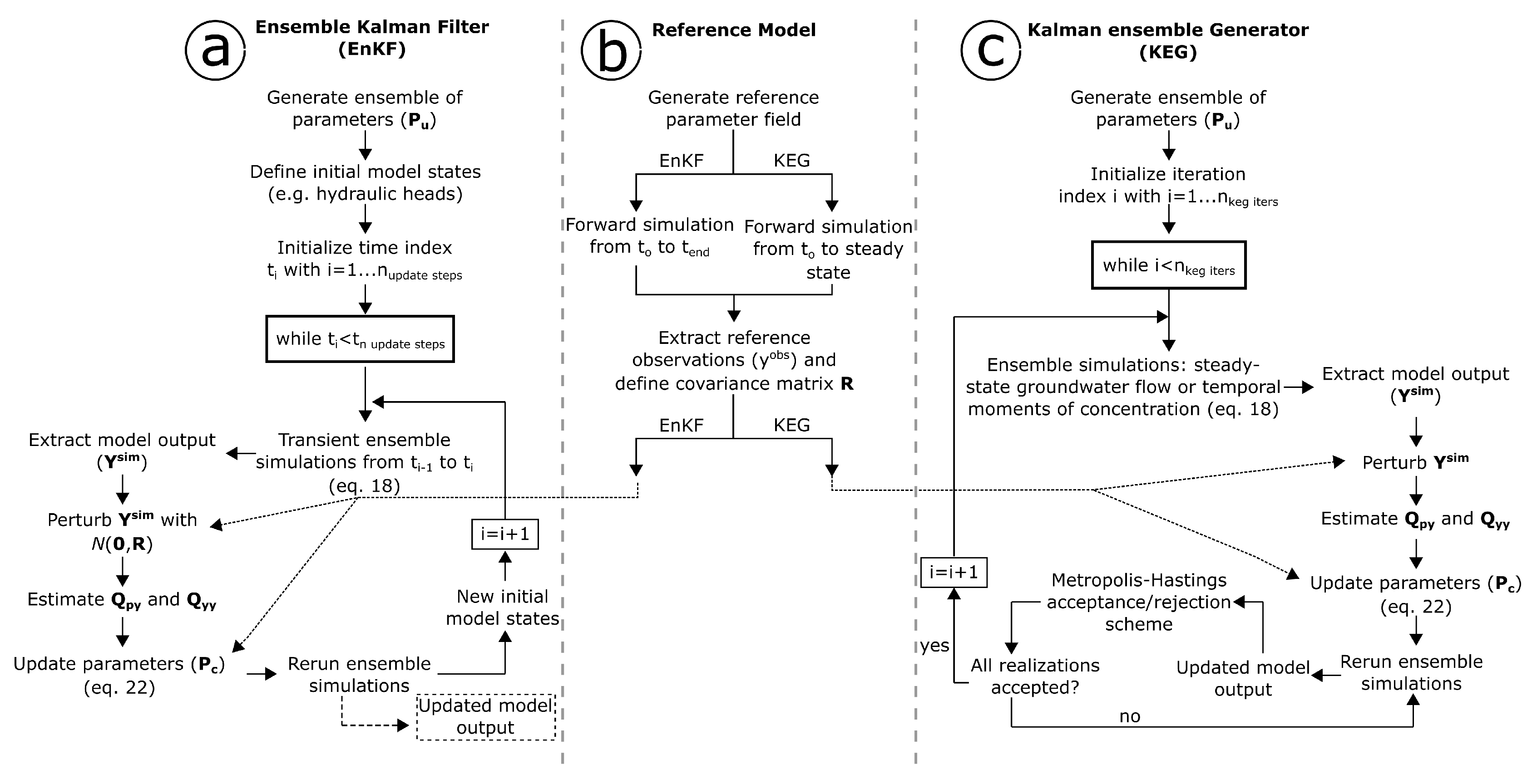
3. Parameter Estimation with Ensemble Kalman-Based Methods

The Kalman filter was first introduced to describe a recursive solution of the linear filtering problem [86]. In each time step, all states of the model are updated, minimizing the sum of squared residuals between measurements and model predictions. Prior knowledge about the states is accounted for in the form of covariance functions between all predicted observations and between states and predicted observations. In its original form, both the predictive model and the measurement operator had to be linear. Several modifications to the filter have been suggested for its application to nonlinear dynamics. In ensemble Kalman-based methods, the covariance matrices are approximated by performing and analyzing an ensemble of model runs [87]. In this work, we applied two different ensemble Kalman-based methods for the estimation of hydraulic-conductivity fields: the Ensemble Kalman Filter and the Kalman Ensemble Generator. Both methods share the same underlying theory, and differ mainly in the way observations are used.
Let us assume a true nonlinear system within an ensemble framework, described by the following stochastic forecast equation:
y t s i m , i = f ( p t 1 i , ϕ t 1 )
in which i = 1 , 2 , , N e n s denotes the index of an individual ensemble member, N e n s is the total number of ensemble members, f is a nonlinear model that simulates the model observations y s i m (e.g., drawdown values or concentrations), p is a vector of model parameters (e.g., hydraulic conductivity), t is the time index, and ϕ t 1 are the model states at the previous time. In the case here, we assume that model simulations are affected only by parameter uncertainties. Preceding studies included examples of how to include model uncertainties in the EnKF, which is not considered here [88,89,90]. For compatibility with the real observations y o b s , measurement noise ϵ drawn from a multi-Gaussian probability distribution with zero mean and covariance matrix R is added to the simulated observations y t s i m , i [35]. Dropping the time index t for clarity, the ensemble estimate of the ( N p a r × N o b s ) cross-covariance matrix Q p y between model parameters and modeled observations can be estimated by
Q p y 1 N e n s 1 ( P P ¯ ) ( Y s i m Y ¯ s i m ) T
and the ( N o b s × N o b s ) autocovariance of modeled observations Q y y is estimated from the ensemble as
Q y y 1 N e n s 1 ( Y s i m Y ¯ s i m ) ( Y s i m Y ¯ s i m ) T
in which P is the ( N p a r × N e n s ) matrix containing all model parameters of all ensemble members, and Y s i m is the ( N o b s × N e n s ) matrix composed of the vectors of modeled observations of all ensemble members. The overbar represents the ensemble average of the corresponding matrices, e.g.,
Y ¯ i , k s i m = 1 N e n s j = 1 N e n s Y i , j s i m k ( 1 , 2 , , N e n s )
Equations (19) and (20) imply that the approximations of the covariance matrices improve with increasing ensemble size. In the linear case, the ensemble Kalman-based methods for parameter estimation converge to the result of the classical Kalman filter in the limit of an infinite ensemble size. After computing the matrices Q p y and Q y y , the parameters of the ensemble member i are updated according to the analysis equation:
p c i = p u i + β Q p y ( Q y y + R ) 1 ( y o b s ( y s i m , i + ϵ i ) )
in which the subscripts u and c refer to the unconditional and conditional parameters contained in P , respectively, and β is a damping factor between 0 and 1. This damping factor reduces the parameter change upon the update, mitigating the known issue of filter inbreeding [23,33], in which the ensemble variance of parameters erroneously collapses after a few update cycles. Equation (22) states that the posterior (or conditional) ensemble member p c i is a linear combination of the prior (or unconditional) ensemble member p u i plus an update term that is proportional to the difference between the actual measurement and the associated model prediction.
An underlying assumption in ensemble Kalman-based methods is that all variables involved (i.e., parameters, model states, and observations) are random functions following a multi-Gaussian distribution, and therefore are fully characterized by their mean and covariance matrix. This implies that the relationship between the independent parameters and the dependent variables is linear. The latter assumption is justified for groundwater flow and solute transport applications only under idealized boundary conditions [91]. Effects of nonlinearities are mitigated, to some extent, by the application of the damping factor β in the analysis Equation (22). To further reduce the impact of non-Gaussianity, one may transform the model states and parameters such that their marginal distributions become Gaussian (normal-score transformations or Gaussian anamorphosis) [39,92,93]. The normal-score transformation is a monotonically increasing univariate transformation that modifies the shape of the probability density function on a marginal level, without changing the statistical dependence and thus without ensuring multi-Gaussianity after the transformation. As highlighted in several studies [27,39], normal-score transformations have to be used with caution as their application to data with a strongly nonlinear dependence on the parameters may introduce artifacts that corrupt the numerical covariances. According to Schöniger et al. [39], transformed variables are included in the analysis equation as follows,
p c i = p u i + Q p y ^ Q yy + R ^ 1 y o b s ^ ( y s i m , i + ϵ i ^ )
in which the hat symbol represents transformed variables. We built an individual transformation function for each measurement location [94] and applied it to both the perturbed modeled observations ( y s i m , i + ϵ i ) and the corresponding reference observation. After parameter updating, back transformation of model observations is not required as they are computed by additional model runs with updated parameters at the new time step [39].
In the standard update scheme of the EnKF, the parameters and/or model states are updated by evaluating the model performance at one step forward in time. The updated states and parameters are then used as initial condition for the next step [22,26,39,92,95,96,97], and the process finalizes once all available data are assimilated.
We applied this version of the filter to the assimilation of transient hydraulic-head data. Other authors have also used this version to estimate parameters from concentration data [25,98]. This classical update scheme of the EnKF, however, leads to mass balance errors when assimilating transient concentration data, mainly due to inconsistencies between the predefined steady-state flow field and the updated hydraulic parameters. To honor mass conservation and consistency between hydraulic parameters and concentrations during the assimilation of concentration data, we reinitialized the steady-state flow model after each parameter update and resimulated transport from the initial time until the next available measurement time step. This version of the filter is known as the restart EnKF [23,27,29,99]. The computational effort of this scheme scales with the squared number of measurement times.
In contrast to the EnKF, parameter updating in the Kalman Ensemble Generator (KEG) is performed by assimilating all observations simultaneously [38], as it is usually done in a batch calibration. This update scheme requires an iterative approach where the same data are reused to update those ensemble members in which the likelihood of the data does not meet a convergence criterion. We implemented the Metropolis–Hastings algorithm with variance inflation as the acceptance/rejection sampling scheme. In this scheme, we compute for each ensemble member i, the critical CDF value P r i in the χ 2 distribution, for an objective function defined by χ i 2 = r i T R 1 r i , where the residuals r i are the difference between reference and simulated observations for member i ( y o b s ( y s i m , i + ϵ i ) ) . If P r i is smaller than a random number drawn from the interval [ 0 , 1 ], the member i is accepted as part of the conditional ensemble. All rejected realizations are repeatedly updated according to Equation (22), but with an artificially increased measurement variance. The corresponding models are resimulated, and the values P r i are reevaluated, until all realization are accepted, or a predefined maximum number of iterations is reached.
In our application of the KEG, we updated parameters using only steady-state drawdown values due to pumping. For the assimilation of tracer data, we recomputed the steady-state hydraulic head field prior to any transport simulation, and used the mean breakthrough time (that is, the ratio of the first over the zeroth temporal moment of concentration) as data. The reason for using the KEG when assimilating steady-state heads and temporal moments of concentrations is that the number of data is much smaller than in the assimilation of time series. In the EnKF, convergence of parameters is typically achieved after many data assimilation cycles referring to different measurement time points. When assimilating steady-state values or temporal moments, cycling over consecutive time steps is not possible and convergence must be achieved upon iterations in the assimilation of the same limited data set.
Figure 1 summarizes the forecast/update scheme of both ensemble Kalman-based methods presented. The steps to update the parameters with the EnKF are shown in column a of the figure, and the update scheme of the KEG is presented in column c. Column b refers to the general steps to generate a reference model, emphasizing that the same set of parameters are used for generating synthetic data with the two different numerical models applied in this work.

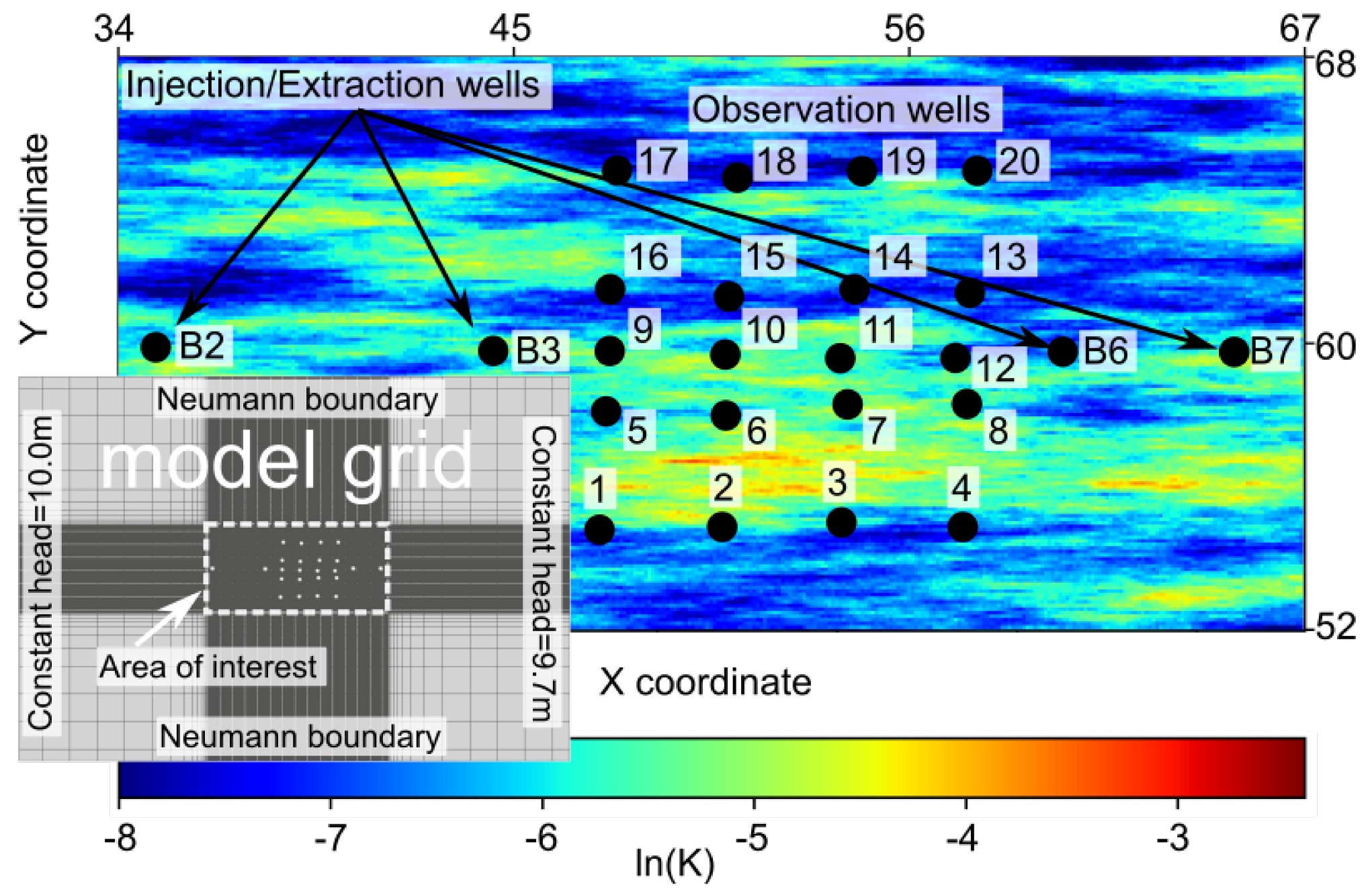
4. Numerical Implementation of a Synthetic Tomographic Experiment

To assess the performance of the EnKF and KEG in the context of hydraulic and tracer tomography experiments, we created synthetic tests with 2-D numerical models. For the EnKF we used the pde-based hydrological model HydroGeoSphere (Aquanty, Waterloo, ON, Canada, ref. [76]). HydroGeoSphere solves the groundwater flow equation (Equation (1)) and the dual-domain version of the advection–dispersion equation (Equation (12)) using the Finite Element Method. The model set-up, presented in Figure 2, consists of a grid with 132,090 nodes and 65,504 elements, covering an area of 100 × 70 m. The model domain was divided into two regions with different grid resolutions. The smallest elements ( Δ x = Δ y = 0.1 m) were generated within the region where the extraction, injection, and observation wells are located. In the following, we refer to this part of the domain as the area of interest. The elements were coarsened toward the domain boundaries, reaching a maximum element size of 5 × 5 m.
Constant hydraulic heads of 10 m and 9.7 m were defined at the left and right boundaries of the domain, respectively, generating an ambient hydraulic gradient of 0.3 % . No-flow conditions were assigned to the upper and lower boundaries, and an initial concentration of zero was defined all over the model domain at the beginning of the simulations.
We generated the reference field of log-hydraulic conductivity in the area of interest (ln(K), Figure 2) using a spectral approach [100], and a geostatistical model based on hydraulic conductivity values reported for the hydrogeological research site Lauswiesen (exponential model, mean hydraulic conductivity μ K = 3.0 × 10 3 ms 1 , variance of ln(K) σ l n ( K ) 2 = 1, and longitudinal and transverse correlation lengths I l = 8 m and I t = 1 m, respectively) [101]. All elements outside the area of interest were assigned a value equal to the mean ln(K) of the geostatistical model, and were treated as a single value during parameter updating, leading to a considerable reduction of matrix dimensions. The given transport parameters were also based on previous field investigations performed at the Lauswiesen site [62,102]. Storativity ( S o ) and longitudinal dispersivity ( α l ) were assumed homogeneous and equal to 3.5 × 10 3 m 1 and 1 m, respectively. The dual-domain transport model was implemented with a mass transfer coefficient λ m t = 1 × 10 9 s 1 , immobile porosity of n i m = 20 % , and a porosity value for the mobile zone n m = 10 % .
As mentioned before, we updated parameters with the KEG using only steady-state hydraulic heads and the mean tracer arrival times. For that, we generated an additional two-dimensional groundwater flow and concentration-moment generating model that directly solves for steady-state hydraulic heads and temporal moments of tracer concentration. In this model, all partial differential equations are solved by the Finite Volume Method on rectangles, and upwind differentiation is applied to stabilize advection-dominated transport. The model domain was limited to the extension of the area of interest in Figure 2. All additional settings such as grid spacing, type of boundary conditions, ambient hydraulic gradient, and hydraulic conductivities were the same as for the HydroGeoSphere model.
In both models, we simulated a nested-cell flow field with two injection and two extraction wells [16,70,103]. A total of 20 observation wells was distributed in the area between the inner injection and extraction points. The injection and extraction wells were labeled B2, B3, B6, and B7, and the observation wells were consecutively numbered between 1 and 20, starting from left to right and bottom to top (see Figure 2). Because the test model was two-dimensional, we could not account for different injection or observation depths, as it might be the case in field applications. Instead, the tomographic layout was achieved by inverting the injection and extraction wells (inverted flow field) and changing the location of the tracer injection from well B3 to well B6. The location of the extraction, injection and observation wells was set to match that of the well field at the Lauswiesen site.
We performed flow and transport simulations sequentially. With the HydroGeoSphere model, we first simulated transient groundwater flow with the two injection and two extraction wells until steady-state flow was achieved. For transport, we used the final steady-state flow-field and simulated solute transport with the injection of a conservative tracer at the selected well (i.e., well B3 or B6). In the Matlab implementation, we first solved for steady-state groundwater flow with the same two injection and two extraction wells, and then used the calculated field to solve for the first two temporal moments of tracer concentration. Table 1 contains the injection/extraction rates and the tracer mass injected during each test of the synthetic tomographic experiment. The test labels A and B refer to the full sequence of flow and transport simulations. Each individual simulation is identified by a pumping test and tracer test label.
The synthetic transient hydraulic dataset consists of two sets of 20 drawdown curves recorded at 28 time steps. Each set corresponds to one of the two simulated hydraulic tests. The synthetic transient tracer data contains two sets of 22 breakthrough curves measured at all observation wells and the two corresponding extraction wells. The synthetic steady-state hydraulic dataset also consists of two sets but only of the steady-state hydraulic-head values calculated at the 20 observation points. The compressed tracer datasets consist of one set of mean tracer arrival times (i.e., the ratio of the first to the zeroth temporal moments) per tracer test, evaluated at the 20 observation points and the two extraction wells.
Figure 3 shows an example of the drawdown (top) and breakthrough (bottom) curves simulated with pumping and tracer tests B. To mimic measurement uncertainty, we added white noise drawn from a Gaussian distribution ( μ = 0 , σ = measurement error) to the synthetic datasets. The assumed measurement errors for drawdown and concentration data were 1 mm and 10% measurement error relative to the reference value, respectively, and are compatible with the expected accuracy of modern sensors for hydraulic head and tracer concentrations. We observed a maximum drawdown of ~1.2 m during both pumping tests. Negative drawdown was observed at locations close to the injection wells, indicating groundwater mounding caused by water injection.
While the simulated tracer tests relate to a pulse injection, we analyze cumulative concentrations, which would be equivalent to the response to a continuous injection. This leads to a monotonic behavior of the signal, and a monotonic sensitivity with respect to hydraulic parameters. To exemplify this, Figure 4 shows a schematic breakthrough curve for a pulse injection (Figure 4A) and its time integral (Figure 4B) for different velocity values. If the estimated velocity is far off, the true and simulated breakthrough curves practically do not overlap so that a gradual change of velocity hardly changes the sum of squared errors. Figure 4C shows the resulting error norm as a function of the assumed velocity. Only when the initial guess is already good, it is clear how to change the velocity to achieve a better fit. When considering the cumulative breakthrough curve, by contrast, a slight change in the velocity leads to significant changes in the sum of squared errors, even for velocity values that are far off (Figure 4D). The latter implies a larger radius of convergence of the parameter estimation.
We obtained maximum cumulative tracer concentrations of ~40 mgsL 1 in the synthetic tracer tests. For tracer test A, mean tracer arrival times of ~16 h and ~33 h were registered at extraction wells B6 and B7, respectively. For tracer test B, mean arrival times of ~36 h and ~20 h were calculated at the extraction wells B2 and B3, respectively. The shorter mean travel times registered for tracer test A (tracer injection at the upstream well B3) are attributed to the natural hydraulic gradient and the relatively low pumping rates applied at the upstream wells (B2 and B3) during tracer test B, where the enforced flow field was oriented in opposite direction to the ambient flow. In tracer test A, 90% of the tracer mass was recovered, whereas only 82% was recovered in tracer test B. The remaining tracer mass was either released into the natural ambient flow or did not arrive at the extraction wells within the simulated time period.
Examples of the simulations performed with the steady-state groundwater flow model and temporal moments of tracer concentrations are shown in Figure 5, with the reference steady-state hydraulic head field (a) and the mean tracer arrival times distribution (b) for pumping and tracer test A, respectively. For tracer test A, we registered mean tracer arrival times of ~22 h and ~26 h at extraction wells B6 and B7, respectively, which are values similar to those obtained with the transient HydroGeoSphere model.

5. Parameter Estimation with Ensemble Kalman-Based Methods

The sequential parameter estimation started with the assimilation of the synthetic drawdown data of pumping test A followed by drawdown data of pumping test B. We then used the ensemble of parameters conditioned to head data as initial parameter fields for the assimilation of transport data (tracer test A followed by tracer test B). We used an ensemble of 500 random realizations. Hendrick-Franssen and Kinzelbach [23] showed that this ensemble size was appropriate to reduce filter inbreeding problems in groundwater applications. Each realization of the ensemble was initialized using the same geostatistical parameters as in the reference case, thus assuming that we have the correct statistical prior knowledge about the aquifer parameters.
As mentioned above, we used transient hydraulic-heads and cumulative concentration data in the EnKF, updating the parameters at each measurement time. The standard update scheme of the EnKF was applied to drawdown data, and the restart EnKF was used for the assimilation of concentration data. In the KEG, we used the steady-state hydraulic-head (drawdown) values affected by pumping, and the mean tracer arrival times to update the hydraulic conductivity fields. The data simulated at the observation wells were reused for updating those ensemble members in which the likelihood of the data did not meet an acceptance criterion defined by a Metropolis–Hastings scheme. The covariance matrix of the data was adaptively inflated to accelerate convergence. We observed that the cumulative distribution of the objective function (i.e., mean of the normalized squared residuals) stabilized approximately after 10 iterations, regardless of the acceptance rate of the individual ensemble members.
To improve filter performance, we adjusted the settings of the EnKF and KEG such as the damping factor and normal-score transformations of the data. In the following, we discuss only those settings for which we observed the best performance. Table 2 summarizes the main settings applied in each method.
The filter performance was quantified with the mean absolute error (MAE) as a metric for the correctness of the estimated parameter ensemble, the mean ensemble standard deviation (MESD) as a metric of the ensemble spread, and the root mean square error (RMSE) between reference and simulated observations, as a metric of model predictability:
M A E u = 1 G i = 1 G | p ¯ i , u m o d p i r e f |
M E S D u = 1 G M j = 1 M i = 1 G ( p i , j , u m o d p ¯ i , u m o d ) 2
R M S E u = 1 N i = 1 N y ¯ i m o d y i r e f 2
in which u indicates that the analysis is performed for each update step, G is the number of grid elements, M is the number of realizations in the ensemble, p m o d and p r e f refer to the updated and reference parameter value, respectively, the overbar represents the ensemble average, N is the number of observations, and y ¯ i m o d and y i r e f are the i-th ensemble mean and reference observations at each update step, respectively.
The calculation of the mean absolute error (MAE) requires the true parameter values in all grid elements, averaged over all grid elements considered, and therefore it can only be computed in virtual cases where the true parameters are known. The MESD is the mean standard deviation evaluated in all grid elements. According to Hendricks-Franssen and Kinzelbach [23], MESD/MAE ratios smaller than 1 are indicative of filter inbreeding. As mentioned above, predictability was evaluated with the RMSE, where a value of zero would imply a perfect match between modeled and reference (or measured) data.
A key problem of comparing point-values of log-conductivity is that small spatial shifts of otherwise correctly identified patterns can lead to error metrics similar to estimates that miss the patterns altogether. Thus, we further compare the reference and the estimated log-hydraulic conductivity fields with the structural similarity index (SSIM) [104]. This metric is commonly used in image processing to measure the degradation of the structural information of an image (in our case the estimated parameter fields) when compared to the original. The SSIM index between the reference and estimated log-hydraulic conductivity fields, within a specific region defined by a window i of arbitrary size, is computed by
S S I M ( r e f , e s t ) i = ( 2 μ r e f μ e s t + C 1 ) ( 2 σ r e f , e s t + C 2 ) ( μ r e f 2 + μ e s t 2 + C 1 ) ( σ r e f 2 + σ e s t 2 + C 2 )
in which ref and est are the reference and estimated parameter values, respectively, μ r e f and μ e s t are the reference and estimated mean values, respectively, σ r e f and σ e s t are the corresponding variances, σ r e f , e s t is the covariance between reference and estimated values, and C 1 and C 2 are small constants used to stabilize the model when ( μ r e f 2 + μ e s t 2 ) or ( σ r e f 2 + σ e s t 2 ) , respectively, are close to zero. These values are estimated for the region defined by the window i, and a map of the SSIM index covering the entire parameter field is generated by shifting the window. In our case, we chose a window size equal to the longitudinal correlation length used to generate the random parameter fields, and report the mean SSIM index representative for the whole model domain. The SSIM index varies between −1 to 1, where 1 would indicate that the two parameter fields are identical.
In contrast to the MAE, which quantifies the differences between the reference and estimated parameter fields cell-wise, the SSIM index compares structural patterns in local regions of the domain, and is less sensitive to differences caused by small shifts.

6. Results and Discussion

The top row of Figure 6 displays the reference log-hydraulic conductivity field (a), the initial ensemble-mean (b), and the initial ensemble variance (c). Note that the same initial ensemble was used in both ensemble Kalman-based methods. To facilitate a visual comparison of the parameter fields estimated by both methods, Figure 6 also displays the ensemble-mean of log-hydraulic conductivity and associated variance, obtained after all hydraulic-head (d ande) and tracer (f and g) data had been assimilated. In the following, we first discuss the results of the parameter estimation based on hydraulic-head data only, followed by those obtained after the additional assimilation of tracer data. In both methods, the corresponding ensemble conditioned on hydraulic heads was used as the initial ensemble in the assimilation of tracer data.

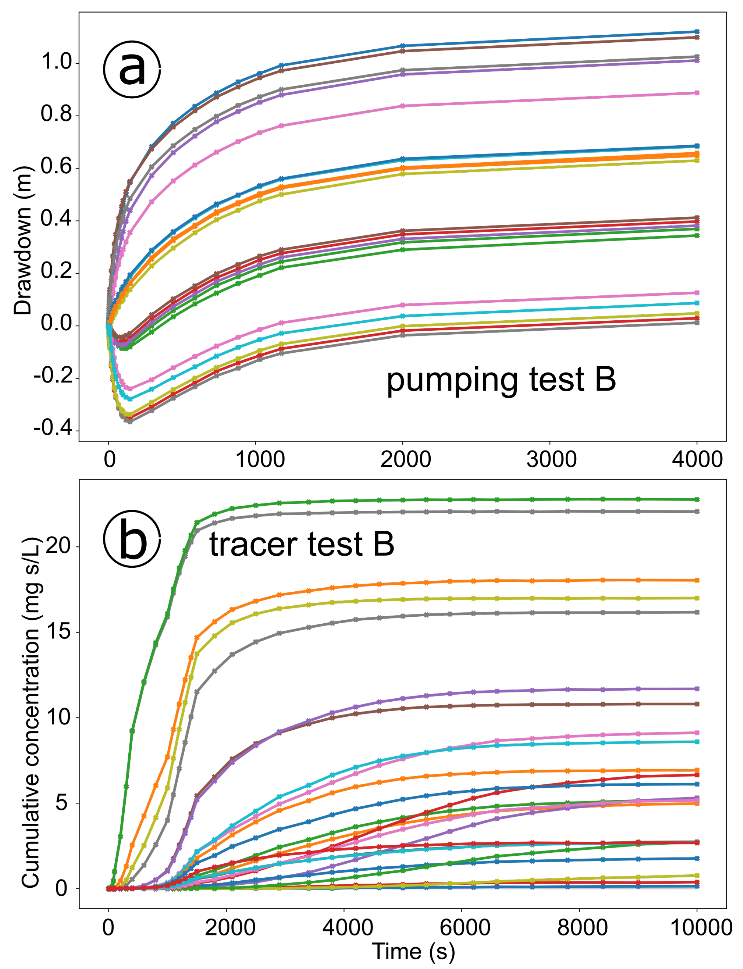
6.1. Assimilation of Drawdown Data

A visual inspection of the log-hydraulic conductivity fields conditioned to hydraulic-head data (Figure 6d,e) reveals that the high hydraulic conductivity zones that are located close to the pumping and observation points, are well recovered by both methods. However, the estimation rapidly deteriorates with distance to the observation points and pumping wells, especially for the KEG. In general, the ensemble mean of log-hydraulic conductivity estimated with the KEG is smoother than for the EnKF, suggesting that steady-state hydraulic head values provide less information of small-scale variations in hydraulic conductivity than transient head data. Improvements in the estimation of parameters with the EnKF were observed when normal-score transformations and a damping factor were applied. We evaluated the individual effects of these tuning settings (results not shown), but a combination of normal-score transformations and damping always outperformed the application of only one of these settings. The best performance was achieved with a damping factor β of 0.1. There is no clear method to define an optimal value for the damping factor β . In the EnKF, Hendrick-Franssen and Kinzelbach [24] recommend using a value of 0.1 in groundwater problems with mildly heterogeneous aquifers (variance of log-K close to 1). The damping factor reduces the perturbation of the parameters in the update, improving pseudolinearizations, however, at the cost of smoother fields. The more time-points of the hydraulic-head time series are assimilated, the more damping is necessary, because the transient heads are strongly correlated in time. The KEG assimilates only steady-state hydraulic heads, therefore damping is not applicable.
The mean absolute error (MAE) of the ensemble-average of the log-hydraulic conductivity field was reduced by ~17% with the EnKF, whereas the same error metric increased by 2% with the KEG (Table 3). We attribute the latter increase to the disagreement between reference and estimated parameters furthest from the pumping wells and observation points. The ensemble spread quantified by the mean ensemble standard deviation (MESD) was reduced by 30% and 16% with the EnKF and KEG, respectively. Small ensemble spreads are not necessarily a sign of successful parameter estimation and can be indicative of filter inbreeding, especially when no similar reduction of the misfit is observed. Filter inbreeding quantified by the MESD/MAE ratio [23] yielded values of 0.92 and 0.89 for the EnKF and KEG, respectively (see Table 3). Average SSIM index values S S I M ¯ of 0.47 and 0.42 were estimated for the ensemble-mean of log-hydraulic conductivity fields obtained with the EnKF and the KEG, respectively, confirming a better representation of the spatial structure of the reference field with the EnKF, but also suggesting that the parameter fields updated with the KEG are not entirely wrong, as implied by the increase of the MAE.
The spatial distribution of the ensemble spread for each method is also shown in Figure 6. In the EnKF, the variance was smoothly reduced within the most sensitive region of the domain (i.e., where data is available). By contrast, the KEG only partially achieved a variance reduction in the area enclosed by the pumping wells and observation points, with a rapid increase of the estimation variance with distance from the observation points.
Figure 7 shows scatterplots of the ensemble-mean and spread of simulated drawdown versus the reference values computed at all observation points, for pumping tests A (Figure 7a) and B (Figure 7b). The transient drawdown records used by the EnKF are shown as black crosses and the steady-state values used by the KEG as red squares. To compare the performance of both methods at the end of the parameter updates, the blue squares in Figure 7 show the drawdown values simulated at the last assimilation time-step with the EnKF, which correspond to the steady-state drawdown values. The ensemble spread in the transient data is shown only for the last assimilation step (blue lines). The estimated root mean square errors were computed for the full transient data in the EnKF, and the steady-state hydraulic heads at the last KEG assimilation iteration.
During the assimilation of data from pumping test A, the steady-state drawdown is better reproduced by the parameter ensemble of the KEG, despite the fewer details of the reference field recovered. If the purpose of the data assimilation is to improve model predictions, these results alone would suggest that no real advantage of the full transient records exist over the steady-state values. However, the parameter ensemble of the EnKF showed less filter inbreeding issues, and a gradual improvement in the predictions was observed after transient data of pumping test B were included. The root mean square errors of the predicted drawdown of pumping test A are larger in the EnKF (~150 mm) than in the KEG (9 mm), but are largely influenced by the misfit observed during the assimilation of early-time drawdown. A considerable reduction is achieved after using data from pumping test B, with RMSE of ~3 mm and ~2 mm for the EnKF and KEG, respectively, which are values close to the assumed measurement error of 1 mm. Biased estimates in drawdown of pumping test A were observed in the EnKF, in which simulated drawdown was mostly underestimated. This bias was corrected to some degree at the end of the assimilation of the drawdown data of pumping test B (blue points in Figure 7b), where the reference values are covered by the ensemble spread (blue lines in Figure 7b).
These results illustrate the importance of the information contained in transient records. Although computationally more demanding, transient data provide valuable information about aquifer heterogeneity, that is missed if data assimilation is based only on steady-state values. Furthermore, aquifer storativity can be incorporated in the estimation only if transient data are included. The latter is important in real applications with transient forcings, in which aquifer storativity is uncertain. As alternative to assimilating full transient drawdown records, temporal moments could be used. The temporal moment-generating equations are steady-state equations with distributed source terms depending on lower-order moments [14].

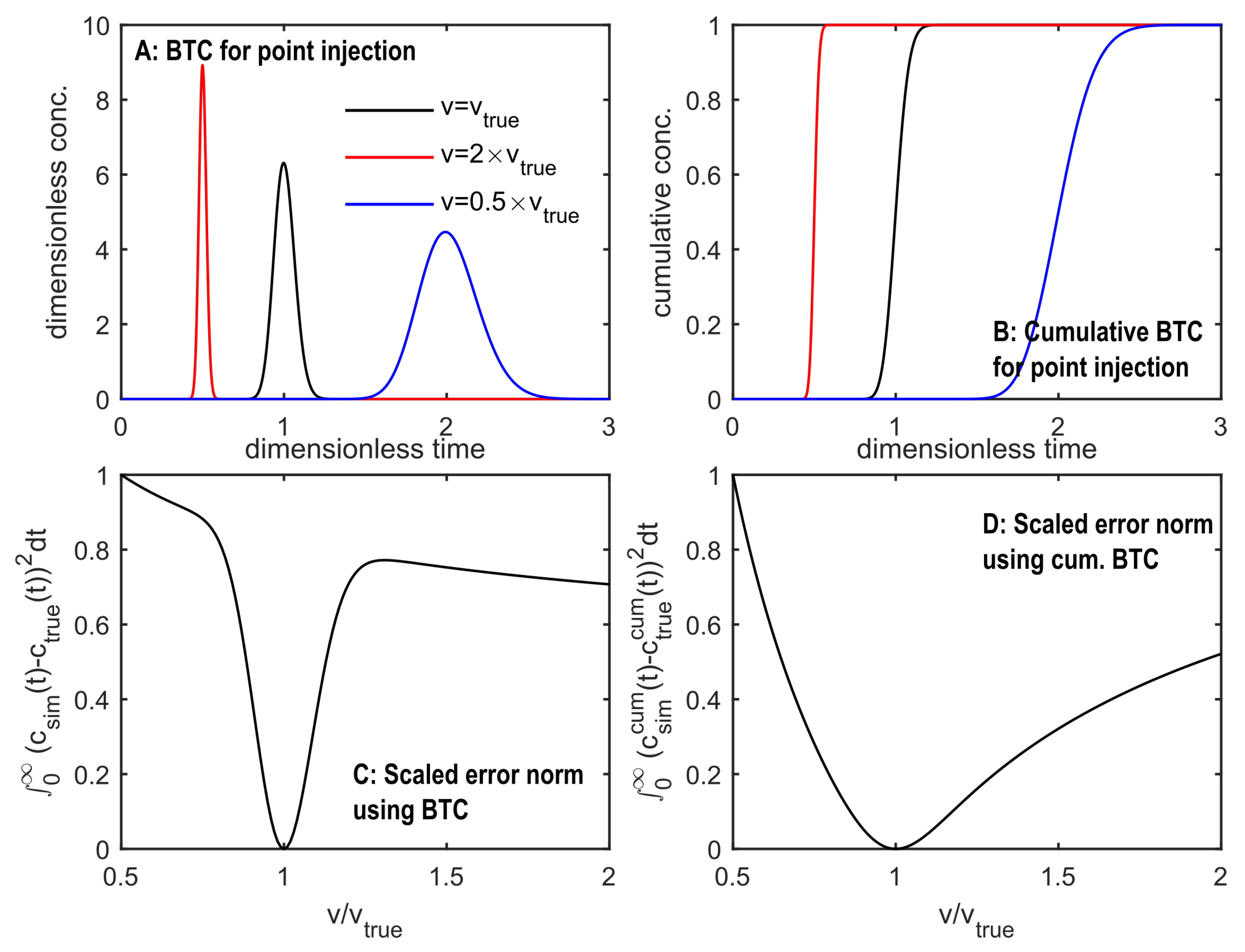
6.2. Sequential Assimilation of Concentration Data

The bottom row in Figure 6 shows the estimated ensemble mean and associated variance of log-hydraulic conductivity after tracer data had been assimilated with the EnKF ( Figure 6f) and the KEG ( Figure 6g). The corresponding initial ensemble mean of log-hydraulic conductivity, that is, those conditioned to drawdown data, are presented in the middle row of Figure 6.
In general, accounting for tracer data helps refining the spatial structure of the parameter fields. For the EnKF, an improvement of the ensemble mean of log-hydraulic conductivity could be observed close to the observation wells, where some of the erroneous low hydraulic conductivity values obtained with the head data were corrected. However, differences between the reference and estimated fields outside this region were amplified, affecting the performance metrics, i.e., an increase of the mean absolute error of log-hydraulic conductivity and a decrease in the average structural similarity index (see Table 4). The reduction in the ensemble variance was not constrained to the region where data is available, indicating some degree of filter inbreeding. This is quantitatively confirmed by the estimated MESD and MAE values of 0.46 and 0.62, respectively, yielding an MESD/MAE ratio for the EnKF of 0.74.
To reduce filter inbreeding and prevent the appearance of extreme parameter values, a stronger damping could be applied, but this would also prevent relevant changes in the parameters and predictions of the simulated observations. In that case, to achieve relevant improvements in the estimation of parameters, more informative data would be required. In real-world applications, additional data could be provided by performing more tracer tests, with the injection and extraction of a tracer solution at different locations. An alternative to a strong damping is to increase the ensemble size. Better approximations of the numerical covariances are obtained with larger ensembles, and therefore the impact of the damping factor becomes less crucial. The ensemble size, however, is constrained by the high computational costs required for transient transport simulations. To further improve the numerical covariances, localization methods may be applied, in which covariances are computed considering only those parameters that are located in regions believed to be sensitive to the data.
Stronger changes could be observed in the ensemble of parameters of the KEG, which were conditioned to the mean tracer arrival times. Some of the small-scale features of the reference field that were missing after the assimilation of hydraulic-head data are better resolved (Figure 6g) after assimilating the mean tracer travel times, especially in the region covered by the observation wells. It is noticeable that the erroneous zone of low hydraulic conductivity developed below the extraction wells B6 and B7 during the assimilation of hydraulic-head data is accentuated in the ensemble mean of log-hydraulic conductivity conditioned to all tracer data. An elongated zone with a strong reduction of the ensemble variance aligns with the injection and extraction wells, and extends all along the y-axis. This behavior has been reported in previous estimations of aquifer parameters based on synthetic tomographic tracer-tests [16], and is closely related to the distinct sensitivity of tracer arrival times on log-hydraulic conductivity [11,12].
We observed a stronger reduction of the ensemble variance in the KEG than in the EnKF, yielding an MESD/MAE ratio of 0.61 (Table 4). The MESD and MAE metrics are affected mainly by the spurious parameter estimates outside the region covered by the observation wells. A decrease in the S S I M ¯ from 0.42 after assimilation of hydraulic data, to 0.40 after using the mean tracer arrival times, suggests that the spatial structure of the ensemble mean of parameters has been slightly deteriorated; however, as for the MESD and MAE, this metric is strongly affected by the wrong estimations outside the region covered by the observation wells.
To assess the prediction capabilities of the parameter fields estimated during the sequential assimilation, we show in Figure 8 scatter plots of the reference cumulative concentrations (a and b) and mean tracer arrival times (c and d) at all observation points, versus the corresponding ensemble mean estimates obtained by the EnKF and KEG, respectively. The ensemble spread of the predictions is represented by the blue and red solid lines. As for the hydraulic-head data, the spread of the predictions with the EnKF is shown only for the last update step. We also report in Figure 8 the root mean square errors (RMSE) and mean absolute errors (MAE) for the predictions by each method. As mean arrival times differ significantly between tracer tests A and B, we report for the KEG a RMSE and MAE normalized by the difference between maximum and minimum arrival times for each test (NRME and NMAE).
In general, both methods show acceptable ensemble predictions during the assimilation of data from tracer test A. Both methods benefit from the inclusion of data from tracer test B, showing a reduction of the RMSE and MAE after all data were assimilated. The bias observed in the EnKF predictions at the end of tracer test A, in which the reference values are mainly underestimated by the ensemble simulations, is not observed for tracer test B. Furthermore, the ensemble spread at the last assimilation step (blue lines in Figure 8) encompasses the reference values at all observation points.
Acceptable mean ensemble predictions are observed for the KEG, especially for tracer test B. The largest ensemble spreads occur at larger mean arrival times and correspond to the observation points 4, 17, and 20, which are located at the corners of the 5 × 4 grid of observation points (see Figure 2). At these locations, the ensemble variance of log-conductivity is also relatively high in comparison to the central region of the domain.
The loss of information in parameter estimation schemes that are based only on low-order temporal moments has been thoroughly studied [12,50,85,105]. In this work, we show that in the context of tomographic tracer-tests, reasonable parameter estimates are achieved with the KEG by considering only the mean arrival time. Including high-order moments, that is, the spread and skewness of the concentration time series would introduce dependencies on effective longitudinal dispersion coefficients and mass transfer kinetics of dual-domain transport. It is also difficult to define meaningful measurement errors of higher-order moments. While simulation results with the KEG are comparable to those of the EnKF, in which the full transient concentration history was used in the estimation, the computational costs were dramatically reduced.
To test whether parameters conditioned to tracer data could still produce acceptable groundwater-flow predictions, we evaluated the transient simulations of pumping test A, using both conditional parameter ensembles. Figure 9 compares the reference drawdown values with the ensemble mean of transient drawdown simulated with the ensemble of parameters conditioned with the EnKF (Figure 9a) and the KEG (Figure 9b). In both plots, the black crosses correspond to the ensemble mean of transient drawdown, and the blue and red squares represent the last simulated step of the pumping step, together with the corresponding ensemble spread described by the blue and red error bars. The reported root mean square errors were computed using the full transient dataset.
Acceptable drawdown predictions of pumping test A with both ensembles are corroborated by a RMSE of 4 cm for the EnKF and 9 mm for the KEG. The last reference drawdown values are well captured by the ensemble updated with the EnKF (blue square and lines in Figure 9), with the largest deviations from the reference observed at those locations furthest from the extraction wells (smaller drawdown values). More favorable error metrics were obtained with the ensemble updated with the KEG, with a smaller RMSE and a reduced ensemble spread (red lines in Figure 9). These results suggest that parameter updating benefits more from temporal moments of tracer concentration, than the concentration history itself. We attribute the limited improvements observed with the assimilation of actual concentrations to the strong damping applied, which was necessary to avoid strong filter inbreeding.
Another aspect is that at intermediate times, deviations between cumulative concentrations can be attributed to either different tracer recoveries or different propagation of the tracer. This ambiguity deteriorates the parameter updates. We deliberately took the mean arrival times rather than zeroth and first temporal moments as data because the zeroth moment is known to show unfavorable sensitivity patterns [106,107].

7. Conclusions and Recommendations

In the present study, we assimilated data from synthetic hydraulic and solute tracer tomography tests to test two Ensemble Kalman-based methods—the Ensemble Kalman Filter and the Kalman Ensemble Generator—for the estimation of aquifer parameters. Both methods improved the parameter fields when data from hydraulic and tracer tomographic tests were sequentially assimilated. We have shown that the EnKF with the transient data outperforms the KEG of steady-state data when hydraulic-heads of pumping tests are assimilated, demonstrating that transient heads are more informative of aquifer heterogeneity than steady-state values only.
For the EnKF, we highly recommend considering cumulative breakthrough curves when assimilating concentration data of tracer tests with pulse injection, in order to achieve a monotonic dependence of the analyzed signal on hydraulic conductivity. While implementing normal-score transformations in the EnKF is beneficial in the assimilation of drawdown data, we do not recommend their application when concentration data are used.
We observed that a strong damping factor is needed to stabilize the update and reduce filter inbreeding ( β = 0.1 ) with the EnKF. This implies that large parameter changes are prevented in individual update steps, so that more data are needed to refine the spatial structure of the estimated fields. These additional data could be provided by increasing the number of sequential tests of the hydraulic and tracer tomographic experiments. We also observed that the temporal moments used as data in the KEG were more informative with respect to the hydraulic conductivity distribution than the cumulative tracer concentrations used with the EnKF. Furthermore, considerable reductions of computational demands are achieved by solving for temporal moments of tracer concentrations, rather than simulating transient transport. Using the KEG for assimilating tracer data based on temporal moments, however, requires that the full breakthrough curve is recovered, which is rarely the case in field applications. Incomplete breakthrough curves may introduce large errors in the computed temporal moments, which may be alleviated by performing transient runs but using truncated temporal moments as data during the assimilation. The latter would annul the efficiency of using temporal-moment generating equations.
In the present application, we have not applied localization methods, in which covariances are computed only for restricted combinations of observations and parameters. The arguments of using such techniques lie in generally known sensitivity patterns of heads and concentration data on the log-hydraulic conductivity field. While in a perfect Kalman-based method a lacking sensitivity leads to a cross-covariance of zero, the restricted ensemble size of any ensemble-based application may cause erroneous correlations that deteriorate the quality of the update step in the filter.
A main drawback of ensemble Kalman-based methods is the necessity of prior knowledge about aquifer parameters (e.g., mean, variance, and correlation structure), which may be limited in real-world applications. This challenge is shared by all methods based on Bayesian inference, and exist also in inversion techniques based on Tikhonov regularization, in which the weights of damping and smoothing terms need to be given. In general, the dependence of the estimated fields on the prior knowledge decreases when more informative data are assimilated, underlying the advantages of tomographic tests. The effects of different cases of prior knowledge in the estimation of parameters with ensemble Kalman-based methods are explored by [33]. They showed that a wrong prior mean, variance, and correlation lengths of parameter fields and groundwater recharge, could lead to aliasing, in which undetected features of hydraulic conductivity are traded for erroneous fluctuations in recharge. In a future work, in which we have applied the EnKF and KEG to real data collected during a field hydraulic and tracer tomographic test, we account for the uncertaintity in the prior knowledge by randomizing the mean, variance, and correlation lengths during the generation of the initial ensemble of hydraulic conductivity fields.

Author Contributions

Conceptualization, E.S.-L. and O.A.C.; methodology, E.S.-L., D.E., and O.A.C.; software, E.S.-L. and O.A.C.; validation, E.S.-L.; formal analysis, E.S.-L.; investigation, E.S.-L.; resources, O.A.C.; data curation, E.S.-L.; writing—original draft preparation, E.S.-L.; writing—review and editing, D.E., C.L., and O.A.C.; visualization, E.S.-L.; supervision, C.L. and O.A.C.; funding acquisition, O.A.C. All authors have read and agreed to the published version of the manuscript.

Funding

This research was funded by the German Research Foundation (DFG) in the framework of the Research Unit 2131 “Data Assimilation for Improved Characterization of Fluxes across Compartmental Interfaces” and the Collaborative Research Center SFB 1253 “CAMPOS—Catchments as Reactors”, Project P7 (Grant Agreements Ci 26/13-2 and SFB 1253/1 2017). The first author also acknowledges the support by the Mexican National Council for Science and Technology (CONACYT). We acknowledge support by Open Access Publishing Fund of University of Tübingen.

Conflicts of Interest

The authors declare no conflicts of interest.

References

  1. Hendricks Franssen, H.J.; Alcolea, A.; Riva, M.; Bakr, M.; Van der Wiel, N.; Stauffer, F.; Guadagnini, A. A comparison of seven methods for the inverse modelling of groundwater flow. Application to the characterisation of well catchments. Adv. Water Resour. 2009, 32, 851–872. [Google Scholar] [CrossRef]
  2. Zhou, H.; Gómez-Hernández, J.J.; Li, L. Inverse methods in hydrogeology: Evolution and recent trends. Adv. Water Resour. 2014, 63, 22–37. [Google Scholar] [CrossRef] [Green Version]
  3. Kitanidis, P.K. Persistent questions of heterogeneity, uncertainty, and scale in subsurface flow and transport. Water Resour. Res. 2015, 51, 5888–5904. [Google Scholar] [CrossRef]
  4. De Marsily, G.; Lavedan, G.; Boucher, M.; Fasanino, G. Interpretation of interference tests in a well field using geostatistical techniques to fit the permeability distribution in a reservoir model. Geostat. Nat. Resour. Charact. 1984, 2, 831–849. [Google Scholar] [CrossRef]
  5. RamaRao, B.S.; LaVenue, A.M.; De Marsily, G.; Marietta, M.G. Pilot point methodology for automated calibration of an ensemble of conditionally simulated transmissivity fields: 1. Theory and computational experiments. Water Resour. Res. 1995, 31, 475–493. [Google Scholar] [CrossRef]
  6. Doherty, J.E. Ground water model calibration using pilot points and regularization. Ground Water 2003, 41, 170–177. [Google Scholar] [CrossRef]
  7. Tsai, F.T.C.; Yeh, W.W.G. Characterization and identification of aquifer heterogeneity with generalized parameterization and Bayesian estimation. Water Resour. Res. 2004, 40. [Google Scholar] [CrossRef] [Green Version]
  8. Kitanidis, P.K. Quasi-linear geostatistical theory for inversing. Water Resour. Res. 1995, 31, 2411–2419. [Google Scholar] [CrossRef]
  9. Gómez-Hernánez, J.J.; Sahuquillo, A.; Capilla, J. Stochastic simulation of transmissivity fields conditional to both transmissivity and piezometric data—I. Theory. J. Hydrol. 1997, 203, 162–174. [Google Scholar] [CrossRef]
  10. Zimmerman, D.A.; De Marsily, G.; Gotway, C.A.; Marietta, M.G.; Axness, C.L.; Beauheim, R.L.; Bras, R.L.; Carrera, J.; Dagan, G.; Davies, P.B.; et al. A comparison of seven geostatistically based inverse approaches to estimate transmissivities for modeling advective transport by groundwater flow. Water Resour. Res. 1998, 34, 1373–1413. [Google Scholar] [CrossRef] [Green Version]
  11. Cirpka, O.A.; Kitanidis, P.K. Sensitivity of temporal moments calculated by the adjoint-state method and joint inversing of head and tracer data. Adv. Water Resour. 2000, 24, 89–103. [Google Scholar] [CrossRef]
  12. Nowak, W.; Cirpka, O. Geostatistical inference of hydraulic conductivity and dispersivities from hydraulic heads and tracer data. Water Resour. Res. 2006, 42, W08416. [Google Scholar] [CrossRef] [Green Version]
  13. Sun, N.Z.; Yeh, W.W.G. Coupled inverse problems in groundwater modeling: 1. Sensitivity analysis and parameter identification. Water Resour. Res. 1990, 26, 2507–2525. [Google Scholar] [CrossRef]
  14. Li, W.; Nowak, W.; Cirpka, O. Geostatistical inverse modeling of transient pumping tests using temporal moments of drawdown. Water Resour. Res. 2005, 41. [Google Scholar] [CrossRef] [Green Version]
  15. Pollock, D.; Cirpka, O.A. Temporal moments in geoelectrical monitoring of salt tracer experiments. Water Resour. Res. 2008, 44. [Google Scholar] [CrossRef] [Green Version]
  16. Schwede, R.L.; Li, W.; Leven, C.; Cirpka, O.A. Three-dimensional geostatistical inversion of synthetic tomographic pumping and heat-tracer tests in a nested-cell setup. Adv. Water Resour. 2014, 63, 77–90. [Google Scholar] [CrossRef]
  17. Kitanidis, P.K.; Lee, L. Principal Component Geostatistical Approach for large-dimensional inverse problems. Water Resour. Res. 2014, 50, 5428–5443. [Google Scholar] [CrossRef] [Green Version]
  18. Lee, J.; Kitanidis, P.K. Large-scale hydraulic tomography and joint inversion of head and tracer data using the Principal Component Geostatistical Approach (PCGA). Water Resour. Res. 2014, 50, 5410–5427. [Google Scholar] [CrossRef]
  19. Zha, Y.; Yeh, T.C.J.; Illman, W.A.; Zeng, W.; Zhang, Y.; Sun, F.; Shi, L. A reduced-order successive linear estimator for geostatistical inversion and its application in hydraulic tomography. Water Resour. Res. 2018, 54, 1616–1632. [Google Scholar] [CrossRef]
  20. Yeh, T.C.J.; Jin, M.; Hanna, S. An iterative stochastic inverse method: Conditional effective transmissivity and hydraulic head ields. Water Resour. Res. 1996, 32, 85–92. [Google Scholar] [CrossRef] [Green Version]
  21. Park, E. A geostatistical evolution strategy for subsurface characterization: Theory and validation through hypotheticaltTwo-dimensional hydraulic conductivity fields. Water Resour. Res. 2020, 56. [Google Scholar] [CrossRef]
  22. Chen, Y.; Zhang, D. Data assimilation for transient flow in geologic formations via ensemble Kalman filter. Adv. Water Resour. 2006, 29, 1107–1122. [Google Scholar] [CrossRef]
  23. Hendricks Franssen, H.J.; Kinzelbach, W. Real-time groundwater flow modeling with the Ensemble Kalman Filter: Joint estimation of states and parameters and the filter inbreeding problem. Water Resour. Res. 2008, 44, W09408. [Google Scholar] [CrossRef]
  24. Hendricks Franssen, H.J.; Kinzelbach, W. Ensemble Kalman filtering versus sequential self-calibration for inverse modelling of dynamic groundwater flow systems. J. Hydrol. 2009, 365, 261–274. [Google Scholar] [CrossRef]
  25. Li, L.; Zhou, H.; Gómez-Hernández, J.J.; Hendricks Franssen, H.J. Jointly mapping hydraulic conductivity and porosity by assimilating concentration data via ensemble Kalman filter. J. Hydrol. 2012, 428, 152–169. [Google Scholar] [CrossRef] [Green Version]
  26. Tong, J.; Hu, B.X.; Yang, J. Assimilating transient groundwater flow data via a localized ensemble Kalman filter to calibrate a heterogeneous conductivity field. Stoch. Environ. Res. Risk Assess. 2012, 26, 467–478. [Google Scholar] [CrossRef]
  27. Crestani, E.; Camporese, M.; Baú, D.; Salandin, P. Ensemble Kalman filter versus ensemble smoother for assessing hydraulic conductivity via tracer test data assimilation. Hydrol. Earth Syst. Sci. 2013, 17, 1517–1531. [Google Scholar] [CrossRef] [Green Version]
  28. Panzeri, M.; Riva, M.; Guadagnini, A.; Neuman, S.P. Data assimilation and parameter estimation via ensemble Kalman filter coupled with stochastic moment equations of transient groundwater flow. Water Resour. Res. 2013, 49, 1334–1344. [Google Scholar] [CrossRef]
  29. Tong, J.; Hu, B.X.; Yang, J. Data assimilation methods for estimating a heterogeneous conductivity field by assimilating transient solute transport data via ensemble Kalman filter. Hydrol. Process. 2013, 27, 3873–3884. [Google Scholar] [CrossRef]
  30. Panzeri, M.; Riva, M.; Guadagnini, A.; Neuman, S.P. Comparison of Ensemble Kalman Filter groundwater-data assimilation methods based on stochastic moment equations and Monte Carlo simulation. Adv. Water Resour. 2014, 66, 8–18. [Google Scholar] [CrossRef]
  31. Camporese, M.; Cassiani, G.; Deiana, R.; Salandin, P.; Binley, A. Coupled and uncoupled hydrogeophysical inversions using ensemble Kalman filter assimilation of ERT-monitored tracer test data. Water Resour. Res. 2015, 51, 3277–3291. [Google Scholar] [CrossRef]
  32. Panzeri, M.; Riva, M.; Guadagnini, A.; Neuman, S.P. EnKF coupled with groundwater flow moment equations applied to Lauswiesen aquifer, Germany. J. Hydrol. 2015, 521, 205–216. [Google Scholar] [CrossRef] [Green Version]
  33. Erdal, D.; Cirpka, O.A. Joint inference of groundwater-recharge and hydraulic-conductivity fields from head data using the ensemble Kalman filter. Hydrol. Earth Syst. Sci. 2016, 20, 555–569. [Google Scholar] [CrossRef] [Green Version]
  34. Evensen, G. Sequential data assimilation with a nonlinear quasi-geostrophic model using Monte Carlo methods to forecast error statistics. J. Geophys. Res. Oceans 1994, 99, 10143–10162. [Google Scholar] [CrossRef]
  35. Burgers, G.; Jan van Leeuwen, P.; Evensen, G. Analysis scheme in the Ensemble Kalman Filter. Mon. Weather Rev. 1998, 126, 1719–1724. [Google Scholar] [CrossRef]
  36. Houtekamer, P.L.; Mitchell, H.L. Data assimilation using an Ensemble Kalman Filter technique. Mon. Weather Rev. 1998, 126, 796–811. [Google Scholar] [CrossRef]
  37. Xu, T.; Gómez-Hernández, J.J.; Zhou, H.; Li, L. The power of transient piezometric head data in inverse modeling: An application of the localized normal-score EnKF with covariance inflation in a heterogenous bimodal hydraulic conductivity field. Adv. Water Resour. 2013, 54, 100–118. [Google Scholar] [CrossRef] [Green Version]
  38. Nowak, W. Best unbiased ensemble linearization and the quasi-linear Kalman ensemble generator. Water Resour. Res. 2009, 45, W04431. [Google Scholar] [CrossRef] [Green Version]
  39. Schöniger, A.; Nowak, W.; Hendricks Franssen, H.J. Parameter estimation by ensemble Kalman filters with transformed data: Approach and application to hydraulic tomography. Water Resour. Res. 2012, 48, W04502. [Google Scholar] [CrossRef] [Green Version]
  40. Gottlieb, J.; Dietrich, P. Identification of the permeability distribution in soil by hydraulic tomography. Inverse Probl. 1995, 11, 353–360. [Google Scholar] [CrossRef]
  41. Yeh, T.; Liu, S. Hydraulic tomography: Development of a new aquifer test method. Water Resour. Res. 2000, 36, 2095–2105. [Google Scholar] [CrossRef]
  42. Liu, S.; Yeh, T.; Gardiner, R. Effectiveness of hydraulic tomography: Sandbox experiments. Water Resour. Res. 2002, 38, 5. [Google Scholar] [CrossRef]
  43. Brauchler, R.; Liedl, R.; Dietrich, P. A travel time based hydraulic tomographic approach. Water Resour. Res. 2003, 39, 1370. [Google Scholar] [CrossRef]
  44. Bohling, G.C.; Zhan, X.; Knoll, M.D.; Butler, J.J. Hydraulic tomography and the impact of a priori information: An alluvial aquifer example. Kans Geol. Surv. 2003. Available online: https://ui.adsabs.harvard.edu/abs/2003AGUFM.H21F..06Z/abstract (accessed on 16 July 2020).
  45. Zhu, J.; Yeh, T.C.J. Analysis of hydraulic tomography using temporal moments of drawdown recovery data. Water Resour. Res. 2006, 42, W02403. [Google Scholar] [CrossRef] [Green Version]
  46. Bohling, G.C.; Butler, J.J.; Zhan, X.; Knoll, M.D. A field assessment of the value of steady shape hydraulic tomography for characterization of aquifer heterogeneities. Water Resour. Res. 2007, 43, W05430. [Google Scholar] [CrossRef] [Green Version]
  47. Illman, W.A.; Liu, X.; Craig, A. Steady-state hydraulic tomography in a laboratory aquifer with deterministic heterogeneity: Multi-method and multiscale validation of hydraulic conductivity tomograms. J. Hydrol. 2007, 341, 222–234. [Google Scholar] [CrossRef]
  48. Illman, W.A.; Liu, X.; Takeuchi, S.; Yeh, T.C.J.; Ando, K.; Saegusa, H. Hydraulic tomography in fractured granite: Mizunami Underground Research site, Japan. Water Resour. Res. 2009, 45, W01406. [Google Scholar] [CrossRef] [Green Version]
  49. Xiang, J.; Yeh, T.C.J.; Lee, C.H.; Hsu, K.C.; Wen, J.C. A simultaneous successive linear estimator and a guide for hydraulic tomography analysis. Water Resour. Res. 2009, 45, W02432. [Google Scholar] [CrossRef] [Green Version]
  50. Yin, D.; Illman, W.A. Hydraulic tomography using temporal moments of drawdown recovery data: A laboratory sandbox study. Water Resour. Res. 2009, 45, W01502. [Google Scholar] [CrossRef]
  51. Berg, S.J.; Illman, W.A. Three-dimensional transient hydraulic tomography in a highly heterogeneous glaciofluvial aquifer-aquitard system. Water Resour. Res. 2011, 47, W10507. [Google Scholar] [CrossRef]
  52. Cardiff, M.; Barrash, W. 3-D transient hydraulic tomography in unconfined aquifers with fast drainage response. Water Resour. Res. 2011, 47, W12518. [Google Scholar] [CrossRef] [Green Version]
  53. Hu, R.; Brauchler, R.; Herold, M.; Bayer, P. Hydraulic tomography analog outcrop study: Combining travel time and steady shape inversion. J. Hydrol. 2011, 409, 350–362. [Google Scholar] [CrossRef]
  54. Cardiff, M.; Barrash, W.; Kitanidis, P.K. A field proof-of-concept of aquifer imaging using 3-D transient hydraulic tomography with modular, temporarily-emplaced equipment. Water Resour. Res. 2012, 48, 1–18. [Google Scholar] [CrossRef] [Green Version]
  55. Berg, S.J.; Illman, W.A. Field study of subsurface heterogeneity with steady-state hydraulic tomography. Ground Water 2013, 51, 29–40. [Google Scholar] [CrossRef] [PubMed]
  56. Brauchler, R.; Hu, R.; Hu, L.; Jiménez, S.; Bayer, P.; Dietrich, P.; Ptak, T. Rapid field application of hydraulic tomography for resolving aquifer heterogeneity in unconsolidated sediments. Water Resour. Res. 2013, 49, 2013–2024. [Google Scholar] [CrossRef]
  57. Cardiff, M.; Barrash, W.; Kitanidis, P.K. Hydraulic conductivity imaging from 3-D transient hydraulic tomography at several pumping/observation densities. Water Resour. Res. 2013, 49, 7311–7326. [Google Scholar] [CrossRef] [Green Version]
  58. Jiménez, S.; Brauchler, R.; Bayer, P. A new sequential procedure for hydraulic tomographic inversion. Adv. Water Resour. 2013, 62, 59–70. [Google Scholar] [CrossRef]
  59. Illman, W.A. Hydraulic tomography offers improved imaging of heterogeneity in fractured rocks. Groundwater 2014, 52, 659–684. [Google Scholar] [CrossRef]
  60. Berg, S.J.; Illman, W.A. Comparison of hydraulic tomography with traditional methods at a highly heterogeneous site. Groundwater 2015, 53, 71–89. [Google Scholar] [CrossRef]
  61. Hochstetler, D.; Barrash, W.; Leven, C.; Cardiff, M.; Chidichimo, F.; Kitanidis, P. Hydraulic tomography: Continuity and discontinuity of high-K and low-K zones. Ground Water 2015, in press. [Google Scholar]
  62. Sánchez-León, E.; Leven, C.; Haslauer, C.P.; Cirpka, O.A. Combining 3D hydraulic tomography with tracer tests for improved transport characterization. Groundwater 2016, 54, 498–507. [Google Scholar] [CrossRef]
  63. Luo, N.; Zhao, Z.; Illman, W.A.; Berg, S.J. Comparative study of transient hydraulic tomography with varying parameterizations and zonations: Laboratory sandbox investigation. J. Hydrol. 2017, 554, 758–779. [Google Scholar] [CrossRef] [Green Version]
  64. Zha, Y.; Yeh, T.C.J.; Illman, W.A.; Onoe, H.; Mok, C.M.W.; Wen, J.C.; Huang, S.Y.; Wang, W. Incorporating geologic information into hydraulic tomography: A general framework based on geostatistical approach. Water Resour. Res. 2017, 53, 2850–2876. [Google Scholar] [CrossRef] [Green Version]
  65. Yeh, T.; Mao, D.; Zha, Y.; Hsu, K.; Lee, C.; Wen, J.; Lu, W.; Yang, J. Why hydraulic tomography works? Ground Water 2013, 52, 168–172. [Google Scholar] [CrossRef] [PubMed]
  66. Bohling, G.; Butler, J.J. Inherent limitations of hydraulic tomography. Ground Water 2010, 48, 809–824. [Google Scholar] [CrossRef]
  67. Vasco, D.W.; Datta-Gupta, A. Asymptotic solutions for solute transport: A formalism for tracer tomography. Water Resour. Res. 1999, 35, 1–16. [Google Scholar] [CrossRef]
  68. Yeh, T.C.J.; Zhu, J. Hydraulic/partitioning tracer tomography for characterization of dense nonaqueous phase liquid source zones. Water Resour. Res. 2007, 43, W06435. [Google Scholar] [CrossRef] [Green Version]
  69. Brauchler, R.; Böhm, G.; Leven, C.; Dietrich, P.; Sauter, M. A laboratory study of tracer tomography. Hydrogeol. J. 2013, 21, 1265–1274. [Google Scholar] [CrossRef]
  70. Doro, K.O.; Cirpka, O.A.; Leven, C. Tracer tomography: Design concepts and field experiments using heat as a tracer. Groundwater 2015, 53, 139–148. [Google Scholar] [CrossRef]
  71. Vasco, D.W.; Datta-Gupta, A.; Long, J.C.S. Resolution and uncertainty in hydrologic characterization. Water Resour. Res. 1997, 33, 379–397. [Google Scholar] [CrossRef]
  72. Illman, W.A.; Berg, S.J.; Liu, X.; Massi, A. Hydraulic/partitioning tracer tomography for DNAPL source zone characterization: Small-scale sandbox experiments. Environ. Sci. Technol. 2010, 44, 8609–8614. [Google Scholar] [CrossRef]
  73. Somogyvári, M.; Bayer, P.; Brauchler, R. Travel-time-based thermal tracer tomography. Hydrol. Earth Syst. Sci. 2016, 20, 1885–1901. [Google Scholar] [CrossRef] [Green Version]
  74. Ringel, L.M.; Somogyvári, M.; Jalali, M.; Bayer, P. Comparison of hydraulic and tracer tomography for discrete fracture network inversion. Geosciences 2019, 9, 274. [Google Scholar] [CrossRef] [Green Version]
  75. Somogyvári, M.; Bayer, P. Field validation of thermal tracer tomography for reconstruction of aquifer heterogeneity. Water Resour. Res. 2017, 53, 5070–5084. [Google Scholar] [CrossRef]
  76. Therrien, R.; Sudicky, E.A. Three-dimensional analysis of variably-saturated flow and solute transport in discretely-fractured porous media. J. Contam. Hydrol. 1996, 23, 1–44. [Google Scholar] [CrossRef]
  77. Scheidegger, A.E. General theory of dispersion in porous media. J. Geophys. Res. 1961, 66, 3273–3278. [Google Scholar] [CrossRef]
  78. Berkowitz, B.; Cortis, A.; Dentz, M.; Scher, H. Modeling non-Fickian transport in geological formations as a continuous time random walk. Rev. Geophys. 2006, 44, RG2003. [Google Scholar] [CrossRef] [Green Version]
  79. Swanson, R.D.; Binley, A.; Keating, K.; France, S.; Osterman, G.; Day-Lewis, F.D.; Singha, K. Anomalous solute transport in saturated porous media: Relating transport model parameters to electrical and nuclear magnetic resonance properties. Water Resour. Res. 2015, 51, 1264–1283. [Google Scholar] [CrossRef] [Green Version]
  80. Feehley, C.E.; Zheng, C.; Molz, F.J. A dual-domain mass transfer approach for modeling solute transport in heterogeneous aquifers: Application to the Macrodispersion Experiment (MADE) site. Water Resour. Res. 2000, 36, 2501–2515. [Google Scholar] [CrossRef] [Green Version]
  81. Liu, G.; Zheng, C.; Gorelick, S.M. Evaluation of the applicability of the dual-domain mass transfer model in porous media containing connected high-conductivity channels. Water Resour. Res. 2007, 43, W12407. [Google Scholar] [CrossRef] [Green Version]
  82. Coats, K.H.; Smith, B.D. Dead-end pore volume and dispersion in porous media. Soc. Pet. Eng. 1964, 4, 73–84. [Google Scholar] [CrossRef]
  83. Sardin, M.; Schweich, D.; Leij, F.J.; Van Genuchten, M.T. Modeling the nonequilibrium transport of linearly interacting solutes in porous media: A review. Water Resour. Res. 1991, 27, 2287–2307. [Google Scholar] [CrossRef]
  84. Harvey, C.F.; Gorelick, S.M. Temporal moment-generating equations: Modeling transport and mass transfer in heterogeneous aquifers. Water Resour. Res. 1995, 31, 1895–1911. [Google Scholar] [CrossRef]
  85. Leube, P.C.; Nowak, W.; Schneider, G. Temporal moments revisited: Why there is no better way for physically based model reduction in time. Water Resour. Res. 2012, 48. [Google Scholar] [CrossRef]
  86. Kalman, R.E. A new approach to linear filtering and prediction problems. Trans. ASME J. Basic Eng. 1960, 82, 35–45. [Google Scholar] [CrossRef] [Green Version]
  87. Evensen, G. The Ensemble Kalman Filter: Theoretical formulation and practical implementation. Ocean Dyn. 2003, 53, 343–367. [Google Scholar] [CrossRef]
  88. Erdal, D.; Neuweiler, I.; Wollschläger, U. Using a bias aware EnKF to account for unresolved structure in an unsaturated zone model. Water Resour. Res. 2014, 50, 132–147. [Google Scholar] [CrossRef]
  89. Rasmussen, J.; Madsen, H.; Jensen, K.H.; Refsgaard, J.C. Data assimilation in integrated hydrological modelling in the presence of observation bias. Hydrol. Earth Syst. Sci. 2016, 20, 2103–2118. [Google Scholar] [CrossRef] [Green Version]
  90. Madsen, H.; Canizares, R. Comparison of extended and ensemble Kalman filters for data assimilation in coastal area modelling. Int. J. Numer. Methods Fluids 1999, 31, 961–981. [Google Scholar] [CrossRef]
  91. Schwede, R.L.; Cirpka, O.A.; Nowak, W.; Neuweiler, I. Impact of sampling volume on the probability density function of steady state concentration. Water Resour. Res. 2008, 44, W12433. [Google Scholar] [CrossRef] [Green Version]
  92. Zhou, H.; Gómez-Hernández, J.J.; Hendricks Franssen, H.J.; Li, L. An approach to handling non-Gaussianity of parameters and state variables in ensemble Kalman filtering. Adv. Water Resour. 2011, 34, 844–864. [Google Scholar] [CrossRef] [Green Version]
  93. Bocquet, M.; Pires, C.A.; Wu, L. Beyond Gaussian statistical modeling in geophysical data assimilation. Mon. Weather Rev. 2010, 138, 2997–3023. [Google Scholar] [CrossRef]
  94. Béal, D.; Brasseur, P.; Brankart, J.M.; Ourmières, Y.; Verron, J. Characterization of mixing errors in a coupled physical biogeochemical model of the North Atlantic: Implications for nonlinear estimation using Gaussian anamorphosis. Ocean Sci. 2010, 6, 247–262. [Google Scholar] [CrossRef] [Green Version]
  95. Bailey, R.T.; Baù, D. Ensemble smoother assimilation of hydraulic head and return flow data to estimate hydraulic conductivity distribution. Water Resour. Res. 2010, 46. [Google Scholar] [CrossRef]
  96. Hendricks Franssen, H.J.; Kaiser, H.P.; Kuhlmann, U.; Bauser, G.; Stauffer, F.; Müller, R.; Kinzelbach, W. Operational real-time modeling with ensemble Kalman filter of variably saturated subsurface flow including stream-aquifer interaction and parameter updating. Water Resour. Res. 2011, 47. [Google Scholar] [CrossRef]
  97. Bailey, R.T.; Baù, D. Estimating geostatistical parameters and spatially-variable hydraulic conductivity within a catchment system using an ensemble smoother. Hydrol. Earth Syst. Sci. 2012, 16, 287–304. [Google Scholar] [CrossRef] [Green Version]
  98. Liu, G.; Chen, Y.; Zhang, D. Investigation of flow and transport processes at the MADE site using ensemble Kalman filter. Adv. Water Resour. 2008, 31, 975–986. [Google Scholar] [CrossRef]
  99. Wen, X.H.; Chen, W.H. Real-time reservoir model updating using Ensemble Kalman Filter with confirming option. Soc. Pet. Eng. 2006. [Google Scholar] [CrossRef]
  100. Dietrich, C.R.; Newsam, G.N. A fast and exact method for multidimensional gaussian stochastic simulations. Water Resour. Res. 1993, 29, 2861–2869. [Google Scholar] [CrossRef]
  101. Lessoff, S.C.; Schneidewind, U.; Leven, C.; Blum, P.; Dietrich, P.; Dagan, G. Spatial characterization of the hydraulic conductivity using direct-push injection logging. Water Resour. Res. 2010, 46. [Google Scholar] [CrossRef]
  102. Riva, M.; Guadagnini, L.; Guadagnini, A.; Ptak, T.; Martac, E. Probabilistic study of well capture zones distribution at the Lauswiesen field site. J. Contam. Hydrol. 2006, 88, 92–118. [Google Scholar] [CrossRef] [PubMed]
  103. Luo, J.; Wu, W.; Fienen, M.N.; Jardine, P.M.; Mehlhorn, T.L.; Watson, D.B.; Cirpka, O.A.; Criddle, C.S.; Kitanidis, P.K. A nested-cell approach for in situ remediation. Ground Water 2006, 44, 266–274. [Google Scholar] [CrossRef] [PubMed]
  104. Zhou, W.; Bovik, A.C.; Sheikh, H.R.; Simoncelli, E.P. Image quality assessment: From error visibility to structural similarity. IEEE Trans. Image Process. 2004, 13, 600–612. [Google Scholar] [CrossRef] [Green Version]
  105. Zhu, J.; Yeh, T. Characterization of aquifer heterogeneity using transient hydraulic tomography. Water Resour. Res. 2005, 41. [Google Scholar] [CrossRef]
  106. Schwede, R.L.; Cirpka, O.A. Stochastic evaluation of mass discharge from pointlike concentration measurements. J. Contam. Hydrol. 2010, 111, 36–47. [Google Scholar] [CrossRef] [PubMed]
  107. Schwede, R.L.; Cirpka, O.A. Interpolation of steady-state concentration data by inverse modeling. Groundwater 2010, 48, 569–579. [Google Scholar] [CrossRef]
Figure 1. General description of the forecast/update schemes of the Ensemble Kalman Filter (column a) and the Kalman Ensemble Generator (column c). (column b) refers to the steps for creating a reference model to obtain synthetic data for both ensemble Kalman-based methods.
Geosciences 10 00276 g001
Figure 2. Two-dimensional synthetic log-hydraulic conductivity field (ln(K)) generated for the area of interest, with the injection and extraction wells and observation points (black dots). Inset shows details of the model grid generated for the HydroGeoSphere model, with a refinement within the area of interest (rectangle with a white dotted line).
Geosciences 10 00276 g002
Figure 3. Synthetic drawdown (a) and cumulative breakthrough curves (b) for pumping and tracer test B, respectively.
Geosciences 10 00276 g003
Figure 4. Sensitivity of a pulse-related breakthrough curve (A) and the corresponding time-integrated signal (B), with respect to groundwater velocity. (C): error norm as a function of velocity, between the reference and simulated breakthrough curves. (D): error norm as a function of velocity, between the reference and simulated cumulative breakthrough curves.
Geosciences 10 00276 g004
Figure 5. Steady-state hydraulic head field (a) and mean tracer arrival times (b) for pumping and tracer test A. Black circles: injection/extraction wells. Black squares: observation wells.
Geosciences 10 00276 g005
Figure 6. Top: reference log-hydraulic conductivity field (a), initial ensemble-mean of the log-hydraulic conductivity field (b), and initial ensemble variance of log-K (c). Middle: ensemble-mean of the log-hydraulic conductivity conditioned to all hydraulic-head data and its associated variance, estimated with the EnKF (d) and the KEG (e). Bottom: ensemble-mean of the log-hydraulic conductivity conditioned to all head and tracer data and its associated variance, estimated with the EnKF (f) and the KEG (g). White dots: injection/extraction wells. Black dots: observation points.
Geosciences 10 00276 g006
Figure 7. Calibration plot for the assimilated transient drawdown of pumping tests A (a) and B (b) used with the EnKF (black crosses), and the steady-state drawdown for the last update iteration with the KEG. Blue squares correspond to the last assimilation time-step with the EnKF. RMSE: root mean square errors. Red and blue bars represent the ensemble spread of drawdown simulations.
Geosciences 10 00276 g007
Figure 8. Calibration plot for the assimilated data of tracer test A (a,c) and tracer test B (b,d). Cumulative concentrations were assimilated with the EnK (black crosses, a,b). Blue squares correspond to the last assimilation time-step with the EnKF. Mean tracer arrival times were used with the KEG (red squares, c,d). RMSE: root mean squared error. MAE: mean absolute error. NRMSE and NMAE: RMSE and MAE normalized by the difference between maximum and minimum values.
Geosciences 10 00276 g008
Figure 9. Calibration plot for the ensemble predictions of drawdown from pumping test A after assimilation of all concentration data. (a): ensemble mean of transient drawdown simulated with the EnKF. (b): ensemble mean of transient drawdown simulated with the KEG.
Geosciences 10 00276 g009
Table 1. Settings of the groundwater flow and transport simulations. Negative flow rates denote extraction of water, whereas positive numbers refer to the injection of water.
InjectionTracerApplied Flow Rates (Ls 1 )
TestWellMass (g)B2B3B6B7
AB3106.03.0−4.0−9.0
BB610−9.0−4.03.06.0
Table 2. Settings of the Ensemble Kalman Filter (EnKF) and Kalman Ensemble Generator (KEG) used for the assimilation of hydraulic-head and tracer data. “✓” and “×” indicate whether normal-score transformations were applied or not. Transf: transformation; cum. conc.: cumulative concentration time series.
Pumping Tests A and BTracer Tests A and B
DataDampingDataDamping
MethodTypeTransf.Factor β TypeTransf.Factor β
EnKFtransient0.1cum. conc.×0.1
KEGsteady-state×n.a.arrival times×n.a.
Table 3. Mean absolute error (MAE) of the ensemble-averaged log-K field, mean ensemble standard deviation of log-K (MESD), MESD/MAE ratio, and ensemble-averaged structural similarity index (SSIM) estimated after the assimilation of hydraulic data from pumping tests A and B. EnKF: ensemble Kalman filter. KEG: Kalman ensemble generator.
MAE ln(K)MESD ln(K)MESD/MAE SSIM ¯
Method(K in ms 1 )(K in ms 1 )(–)(–)
initial0.730.791.081.0
EnKF0.610.560.920.47
KEG0.750.670.890.42
Table 4. Mean absolute error (MAE) of the ensemble-averaged log-K field, mean ensemble standard deviation of log-K (MESD), MESD/MAE ratio, and ensemble-averaged structural similarity index (SSIM) estimated after the assimilation the tracer data from tracer tests A and B. EnKF: ensemble Kalman filter. KEG: Kalman ensemble generator.
MAE ln(K)MESD ln(K)MESD/MAE SSIM ¯
Method(K in ms 1 )(K in ms 1 )(–)(–)
initial0.730.791.081.0
EnKF0.620.460.740.43
KEG0.780.480.610.40

