
Open-Access Worldwide Population STR Database Constructed Using High-Coverage Massively Parallel Sequencing Data Obtained from the 1000 Genomes Project
 and
and
Abstract
:
1. Introduction
2. Materials and Methods
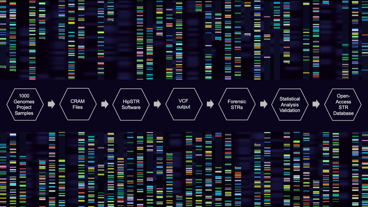
2.1. Genotype Calling
2.2. Statistical Analysis
3. Results
4. Discussion
5. Conclusions
Supplementary Materials
Author Contributions
Funding
Institutional Review Board Statement
Informed Consent Statement
Data Availability Statement
Acknowledgments
Conflicts of Interest
References
- Børsting, C.; Morling, N. Next generation sequencing and its applications in forensic genetics. Forensic Sci. Int. Genet. 2015, 18, 78–89. [Google Scholar] [CrossRef] [PubMed]
- Alvarez-Cubero, M.J.; Saiz, M.; Martínez-García, B.; Sayalero, S.M.; Entrala, C.; Lorente, J.A.; Martinez-Gonzalez, L.J. Next generation sequencing: An application in forensic sciences? Ann. Hum. Biol. 2017, 44, 581–592. [Google Scholar] [CrossRef] [PubMed]
- Ballard, D.; Winkler-Galicki, J.; Wesoły, J. Massive parallel sequencing in forensics: Advantages, issues, technicalities, and prospects. Int. J. Leg. Med. 2020, 134, 1291–1303. [Google Scholar] [CrossRef]
- Auton, A.; Brooks, L.D.; Durbin, R.M.; Garrison, E.P.; Kang, H.M.; Korbel, J.O.; Marchini, J.L.; McCarthy, S.; McVean, G.A.; Abecasis, G.R.; et al. A global reference for human genetic variation. Nature 2015, 526, 68–74. [Google Scholar] [CrossRef] [PubMed] [Green Version]
- Clarke, L.; Fairley, S.; Zheng-Bradley, X.; Streeter, I.; Perry, E.; Lowy, E.; Tassé, A.M.; Flicek, P. The international Genome sample resource (IGSR): A worldwide collection of genome variation incorporating the 1000 Genomes Project data. Nucleic Acids Res. 2017, 45, D854–D859. [Google Scholar] [CrossRef] [PubMed] [Green Version]
- Sudmant, P.H.; Rausch, T.; Gardner, E.J.; Handsaker, R.E.; Abyzov, A.; Huddleston, J.; Zhang, Y.; Ye, K.; Jun, G.; Fritz, M.H.; et al. An integrated map of structural variation in 2,504 human genomes. Nature 2015, 526, 75–81. [Google Scholar] [CrossRef] [PubMed] [Green Version]
- Fungtammasan, A.; Ananda, G.; Hile, S.E.; Su, M.S.; Sun, C.; Harris, R.; Medvedev, P.; Eckert, K.; Makova, K.D. Accurate typing of short tandem repeats from genome-wide sequencing data and its applications. Genome Res. 2015, 25, 736–749. [Google Scholar] [CrossRef] [Green Version]
- Bornman, D.M.; Hester, M.E.; Schuetter, J.M.; Kasoji, M.D.; Minard-Smith, A.; Barden, C.A.; Nelson, S.C.; Godbold, G.D.; Baker, C.H.; Yang, B.; et al. Short-read, high-throughput sequencing technology for STR genotyping. Biotech. Rapid Dispatches 2012, 2012, 1–6. [Google Scholar] [CrossRef]
- Gymrek, M.; Golan, D.; Rosset, S.; Erlich, Y. lobSTR: A short tandem repeat profiler for personal genomes. Genome Res. 2012, 22, 1154–1162. [Google Scholar] [CrossRef] [Green Version]
- Willems, T.; Zielinski, D.; Yuan, J.; Gordon, A.; Gymrek, M.; Erlich, Y. Genome-wide profiling of heritable and de novo STR variations. Nat. Methods 2017, 14, 590–592. [Google Scholar] [CrossRef]
- Fairley, S.; Lowy-Gallego, E.; Perry, E.; Flicek, P. The International Genome Sample Resource (IGSR) collection of open human genomic variation resources. Nucleic Acids Res. 2020, 48, D941–D947. [Google Scholar] [CrossRef] [PubMed]
- Warshauer, D.H.; Lin, D.; Hari, K.; Jain, R.; Davis, C.; Larue, B.; King, J.L.; Budowle, B. STRait Razor: A length-based forensic STR allele-calling tool for use with second generation sequencing data. Forensic Sci. Int. Genet. 2013, 7, 409–417. [Google Scholar] [CrossRef] [PubMed]
- Ganschow, S.; Silvery, J.; Kalinowski, J.; Tiemann, C. toaSTR: A web application for forensic STR genotyping by massively parallel sequencing. Forensic Sci. Int. Genet. 2018, 37, 21–28. [Google Scholar] [CrossRef] [PubMed]
- Valle-Silva, G.; Frontanilla, T.S.; Ayala, J.; Donadi, E.A.; Simões, A.L.; Castelli, E.C.; Mendes-Junior, C.T. Analysis and comparison of the STR genotypes called with HipSTR, STRait Razor and toaSTR by using next generation sequencing data in a Brazilian population sample. Forensic Sci. Int. Genet. 2022, 58, 102676. [Google Scholar] [CrossRef]
- Halman, A.; Oshlack, A. Accuracy of short tandem repeats genotyping tools in whole exome sequencing data. F1000Res 2020, 9, 200. [Google Scholar] [CrossRef] [Green Version]
- Thorvaldsdóttir, H.; Robinson, J.T.; Mesirov, J.P. Integrative Genomics Viewer (IGV): High-performance genomics data visualization and exploration. Brief. Bioinform. 2013, 14, 178–192. [Google Scholar] [CrossRef] [Green Version]
- Robinson, J.T.; Thorvaldsdóttir, H.; Wenger, A.M.; Zehir, A.; Mesirov, J.P. Variant Review with the Integrative Genomics Viewer. Cancer Res. 2017, 77, e31–e34. [Google Scholar] [CrossRef] [Green Version]
- Gettings, K.B.; Ballard, D.; Bodner, M.; Borsuk, L.A.; King, J.L.; Parson, W.; Phillips, C. Report from the STRAND Working Group on the 2019 STR sequence nomenclature meeting. Forensic Sci. Int. Genet. 2019, 43, 102165. [Google Scholar] [CrossRef] [Green Version]
- Peakall, R.; Smouse, P.E. GenAlEx 6.5: Genetic analysis in Excel. Population genetic software for teaching and research-an update. Bioinformatics 2012, 28, 2537–2539. [Google Scholar] [CrossRef] [Green Version]
- Gouy, A.; Zieger, M. STRAF-A convenient online tool for STR data evaluation in forensic genetics. Forensic Sci. Int. Genet. 2017, 30, 148–151. [Google Scholar] [CrossRef]
- Excoffier, L.; Lischer, H.E. Arlequin suite ver 3.5: A new series of programs to perform population genetics analyses under Linux and Windows. Mol. Ecol. Resour. 2010, 10, 564–567. [Google Scholar] [CrossRef] [PubMed]
- Hubisz, M.J.; Falush, D.; Stephens, M.; Pritchard, J.K. Inferring weak population structure with the assistance of sample group information. Mol. Ecol. Resour. 2009, 9, 1322–1332. [Google Scholar] [CrossRef] [PubMed] [Green Version]
- Rosenberg, N.A. Distruct: A program for the graphical display of population structure. Mol. Ecol. Notes 2004, 4, 137–138. [Google Scholar] [CrossRef]
- Jorge, A.; Christopher, P.; Toño, S.; Fernandez, F.L.; Ángel, C.; Maviky, L. pop.STR—An online population frequency browser for established and new forensic STRs. Forensic Sci. Int. Genet. Suppl. Ser. 2009, 2, 361–362. [Google Scholar]
- Tang, H.; Kirkness, E.F.; Lippert, C.; Biggs, W.H.; Fabani, M.; Guzman, E.; Ramakrishnan, S.; Lavrenko, V.; Kakaradov, B.; Hou, C.; et al. Profiling of Short-Tandem-Repeat Disease Alleles in 12,632 Human Whole Genomes. Am. J. Hum. Genet. 2017, 101, 700–715. [Google Scholar] [CrossRef]
- Willems, T.; Gymrek, M.; Highnam, G.; Mittelman, D.; Erlich, Y.; Consortium, G.P. The landscape of human STR variation. Genome Res. 2014, 24, 1894–1904. [Google Scholar] [CrossRef] [Green Version]
- Byrska-Bishop, M.; Evani, U.S.; Zhao, X.; Basile, A.O.; Abel, H.J.; Regier, A.A.; Corvelo, A.; Clarke, W.E.; Musunuri, R.; Nagulapalli, K.; et al. High-coverage whole-genome sequencing of the expanded 1000 Genomes Project cohort including 602 trios. Cell 2022, 185, 3426–3440.e3419. [Google Scholar] [CrossRef] [PubMed]
- West, F.L.; Algee-Hewitt, B.F.B. Cadaveric blood cards: Assessing DNA quality and quantity and the utility of STRs for the individual estimation of trihybrid ancestry and admixture proportions. Forensic Sci. Int. Synerg. 2020, 2, 114–122. [Google Scholar] [CrossRef]
- Pereira, L.; Alshamali, F.; Andreassen, R.; Ballard, R.; Chantratita, W.; Cho, N.S.; Coudray, C.; Dugoujon, J.M.; Espinoza, M.; González-Andrade, F.; et al. PopAffiliator: Online calculator for individual affiliation to a major population group based on 17 autosomal short tandem repeat genotype profile. Int. J. Leg. Med. 2011, 125, 629–636. [Google Scholar] [CrossRef] [Green Version]
- Carratto, T.M.T.; Moraes, V.M.S.; Recalde, T.S.F.; Oliveira, M.L.G.; Teixeira Mendes-Junior, C. Applications of massively parallel sequencing in forensic genetics. Genet. Mol. Biol. 2022, 45, e20220077. [Google Scholar] [CrossRef]
- Yuan, L.; Chen, X.; Liu, Z.; Liu, Q.; Song, A.; Bao, G.; Wei, G.; Zhang, S.; Lu, J.; Wu, Y. Identification of the perpetrator among identical twins using next-generation sequencing technology: A case report. Forensic Sci. Int. Genet. 2020, 44, 102167. [Google Scholar] [CrossRef] [PubMed]
- Diepenbroek, M.; Bayer, B.; Schwender, K.; Schiller, R.; Lim, J.; Lagacé, R.; Anslinger, K. Evaluation of the Ion AmpliSeq™ PhenoTrivium Panel: MPS-Based Assay for Ancestry and Phenotype Predictions Challenged by Casework Samples. Genes 2020, 11, 1398. [Google Scholar] [CrossRef] [PubMed]
- Knijf, P.D. How Next Generation Sequencing Resolved a Difficult Case, Leading to the First Criminal Conviction of Its Kind; Verogen: San Diego, CA, USA, 2020; pp. 1–4. [Google Scholar]
- Pilli, E.; Tarallo, R.; Riccia, P.; Berti, A.; Novelletto, A. Kinship assignment with the ForenSeq™ DNA Signature Prep Kit: Sources of error in simulated and real cases. Sci. Justice 2022, 62, 1–9. [Google Scholar] [CrossRef] [PubMed]
- Cuenca, D.; Battaglia, J.; Halsing, M.; Sheehan, S. Mitochondrial Sequencing of Missing Persons DNA Casework by Implementing Thermo Fisher’s Precision ID mtDNA Whole Genome Assay. Genes 2020, 11, 1303. [Google Scholar] [CrossRef]
- Aalbers, S.E.; Hipp, M.J.; Kennedy, S.R.; Weir, B.S. Analyzing population structure for forensic STR markers in next generation sequencing data. Forensic Sci. Int. Genet. 2020, 49, 102364. [Google Scholar] [CrossRef] [PubMed]
- van der Gaag, K.J.; de Leeuw, R.H.; Hoogenboom, J.; Patel, J.; Storts, D.R.; Laros, J.F.J.; de Knijff, P. Massively parallel sequencing of short tandem repeats-Population data and mixture analysis results for the PowerSeq™ system. Forensic Sci. Int. Genet. 2016, 24, 86–96. [Google Scholar] [CrossRef] [PubMed] [Green Version]
- Verogen. Universal Analysis Software. Available online: https://verogen.com/products/universal-analysis-software/ (accessed on 20 October 2022).
- Scientific, T.F. Precision ID GlobalFiler™ NGS STR Panel v2. Available online: http://www.thermofisher.com/hid-ngs (accessed on 20 October 2022).
- Wang, W.; Wei, Z.; Lam, T.W.; Wang, J. Next generation sequencing has lower sequence coverage and poorer SNP-detection capability in the regulatory regions. Sci. Rep. 2011, 1, 55. [Google Scholar] [CrossRef] [PubMed] [Green Version]
- Sims, D.; Sudbery, I.; Ilott, N.E.; Heger, A.; Ponting, C.P. Sequencing depth and coverage: Key considerations in genomic analyses. Nat. Rev. Genet. 2014, 15, 121–132. [Google Scholar] [CrossRef]
- Castelli, E.C.; Gerasimou, P.; Paz, M.A.; Ramalho, J.; Porto, I.O.P.; Lima, T.H.A.; Souza, A.S.; Veiga-Castelli, L.C.; Collares, C.V.A.; Donadi, E.A.; et al. HLA-G variability and haplotypes detected by massively parallel sequencing procedures in the geographicaly distinct population samples of Brazil and Cyprus. Mol. Immunol. 2017, 83, 115–126. [Google Scholar] [CrossRef] [Green Version]
- Belsare, S.; Levy-Sakin, M.; Mostovoy, Y.; Durinck, S.; Chaudhuri, S.; Xiao, M.; Peterson, A.S.; Kwok, P.Y.; Seshagiri, S.; Wall, J.D. Evaluating the quality of the 1000 genomes project data. BMC Genom. 2019, 20, 620. [Google Scholar] [CrossRef] [Green Version]
- Rosenberg, N.A. A population-genetic perspective on the similarities and differences among worldwide human populations. Hum. Biol. 2011, 83, 659–684. [Google Scholar] [CrossRef]
- Rosenberg, N.A.; Pritchard, J.K.; Weber, J.L.; Cann, H.M.; Kidd, K.K.; Zhivotovsky, L.A.; Feldman, M.W. Genetic structure of human populations. Science 2002, 298, 2381–2385. [Google Scholar] [CrossRef] [PubMed] [Green Version]
- Jobling, M.A. Forensic genetics through the lens of Lewontin: Population structure, ancestry and race. Philos. Trans. R. Soc. Lond. B Biol. Sci. 2022, 377, 20200422. [Google Scholar] [CrossRef] [PubMed]
- de la Puente, M.; Ruiz-Ramírez, J.; Ambroa-Conde, A.; Xavier, C.; Pardo-Seco, J.; Álvarez-Dios, J.; Freire-Aradas, A.; Mosquera-Miguel, A.; Gross, T.E.; Cheung, E.Y.Y.; et al. Development and Evaluation of the Ancestry Informative Marker Panel of the VISAGE Basic Tool. Genes 2021, 12, 1284. [Google Scholar] [CrossRef] [PubMed]
- Phillips, C.; Amigo, J.; Tillmar, A.O.; Peck, M.A.; de la Puente, M.; Ruiz-Ramírez, J.; Bittner, F.; Idrizbegović, Š.; Wang, Y.; Parsons, T.J.; et al. A compilation of tri-allelic SNPs from 1000 Genomes and use of the most polymorphic loci for a large-scale human identification panel. Forensic Sci. Int. Genet. 2020, 46, 102232. [Google Scholar] [CrossRef] [Green Version]
- Lan, Q.; Fang, Y.; Mei, S.; Xie, T.; Liu, Y.; Jin, X.; Yang, G.; Zhu, B. Next generation sequencing of a set of ancestry-informative SNPs: Ancestry assignment of three continental populations and estimating ancestry composition for Mongolians. Mol. Genet. Genom. 2020, 295, 1027–1038. [Google Scholar] [CrossRef]
- Huang, S.; Sheng, M.; Li, Z.; Li, K.; Chen, J.; Wu, J.; Wang, K.; Shi, C.; Ding, H.; Zhou, H.; et al. Inferring bio-geographical ancestry with 35 microhaplotypes. Forensic Sci. Int. 2022, 341, 111509. [Google Scholar] [CrossRef]


| Marker | Lowest Value | Median | Highest Value | Mean | Standard Deviation |
|---|---|---|---|---|---|
| CSF1PO | 21 | 44 | 91 | 44.54 | 8.29 |
| D1S1656 | 24 | 45 | 92 | 45.48 | 8.58 |
| D2S441 | 26 | 49 | 131 | 49.17 | 9.04 |
| D2S1338 | 28 | 50 | 105 | 51.28 | 9.64 |
| D3S1358 | 28 | 51 | 119 | 51.73 | 9.33 |
| D5S818 | 20 | 42 | 98 | 42.90 | 8.14 |
| D7S820 | 20 | 38 | 86 | 39.00 | 7.78 |
| D8S1179 | 26 | 47 | 96 | 48.09 | 8.95 |
| D10S1248 | 18 | 40 | 100 | 40.75 | 7.99 |
| D12S391 | 26 | 52 | 113 | 52.53 | 9.47 |
| D13S317 | 11 | 37 | 79 | 37.93 | 7.50 |
| D16S539 | 21 | 44 | 92 | 44.70 | 8.49 |
| D18S51 | 24 | 47 | 91 | 47.38 | 9.07 |
| D19S433 | 19 | 45 | 89 | 45.28 | 8.62 |
| D22S1045 | 22 | 49 | 111 | 49.47 | 9.11 |
| FGA | 23 | 50 | 118 | 51.33 | 9.49 |
| Penta D | 19 | 43 | 95 | 43.71 | 8.74 |
| Penta E | 18 | 41 | 107 | 41.49 | 8.04 |
| TH01 | 16 | 40 | 83 | 40.73 | 8.01 |
| TPOX | 15 | 37 | 86 | 37.14 | 7.66 |
| vWA | 21 | 47 | 105 | 48.44 | 9.36 |
| Allele | CSF1PO | D1S1656 | D2S441 | D2S1338 | D3S1358 | D5S818 | D7S820 | D8S1179 | D10S1248 | D12S391 | D13S317 | D16S539 | D18S51 | D19S433 | D22S1045 | FGA | Penta D | Penta E | TH01 | TPOX | vWA |
|---|---|---|---|---|---|---|---|---|---|---|---|---|---|---|---|---|---|---|---|---|---|
| 5 | 0.0002 | 0.0125 | 0.0861 | 0.0020 | |||||||||||||||||
| 6 | 0.0004 | 0.0002 | 0.0004 | 0.0034 | 0.0017 | 0.1905 | 0.0210 | ||||||||||||||
| 7 | 0.0198 | 0.0002 | 0.0118 | 0.0178 | 0.0002 | 0.0018 | 0.0004 | 0.0002 | 0.0150 | 0.1084 | 0.2828 | 0.0074 | |||||||||
| 7.3 | 0.0002 | ||||||||||||||||||||
| 8 | 0.0218 | 0.0080 | 0.0006 | 0.0002 | 0.0222 | 0.1842 | 0.0064 | 0.0006 | 0.1394 | 0.0314 | 0.0002 | 0.0006 | 0.0539 | 0.0854 | 0.1287 | 0.4217 | |||||
| 8.3 | 0.0002 | ||||||||||||||||||||
| 9 | 0.0334 | 0.0004 | 0.0018 | 0.0004 | 0.0421 | 0.0942 | 0.0066 | 0.0004 | 0.0891 | 0.1805 | 0.0004 | 0.0012 | 0.0002 | 0.2195 | 0.0358 | 0.2314 | 0.1534 | ||||
| 9.2 | 0.0052 | 0.0016 | 0.0002 | ||||||||||||||||||
| 9.3 | 0.1491 | ||||||||||||||||||||
| 10 | 0.2398 | 0.0080 | 0.2264 | 0.0976 | 0.2534 | 0.0953 | 0.0010 | 0.0763 | 0.1123 | 0.0046 | 0.0028 | 0.0154 | 0.1660 | 0.0873 | 0.0150 | 0.0621 | 0.0004 | ||||
| 10.2 | 0.0004 | 0.0004 | 0.0006 | ||||||||||||||||||
| 10.3 | 0.0002 | 0.0002 | |||||||||||||||||||
| 11 | 0.2658 | 0.0788 | 0.3401 | 0.0004 | 0.3187 | 0.2506 | 0.0753 | 0.0166 | 0.2650 | 0.2888 | 0.0110 | 0.0210 | 0.1649 | 0.1839 | 0.1774 | 0.0002 | 0.2971 | 0.0014 | |||
| 11.2 | 0.0004 | 0.0002 | 0.0008 | ||||||||||||||||||
| 11.3 | 0.0529 | ||||||||||||||||||||
| 11.4 | 0.0002 | ||||||||||||||||||||
| 12 | 0.3375 | 0.0732 | 0.1062 | 0.0022 | 0.3097 | 0.1650 | 0.1180 | 0.0684 | 0.2912 | 0.2336 | 0.0805 | 0.0745 | 0.0170 | 0.1506 | 0.1886 | 0.0359 | 0.0008 | ||||
| 12.2 | 0.0002 | 0.0006 | 0.0122 | ||||||||||||||||||
| 12.3 | 0.0022 | 0.0004 | |||||||||||||||||||
| 13 | 0.0693 | 0.1142 | 0.0282 | 0.0002 | 0.0034 | 0.1841 | 0.0275 | 0.2340 | 0.2616 | 0.0982 | 0.1317 | 0.1155 | 0.2706 | 0.0034 | 0.1380 | 0.1065 | 0.0006 | 0.0072 | |||
| 13.2 | 0.0032 | 0.0341 | |||||||||||||||||||
| 13.3 | 0.0008 | 0.0002 | 0.0002 | ||||||||||||||||||
| 14 | 0.0108 | 0.1472 | 0.2121 | 0.0006 | 0.0777 | 0.0116 | 0.0042 | 0.2418 | 0.2816 | 0.0010 | 0.0370 | 0.0200 | 0.1674 | 0.2726 | 0.0509 | 0.0396 | 0.0669 | 0.0006 | 0.1255 | ||
| 14.2 | 0.0010 | 0.0623 | 0.0002 | 0.0004 | |||||||||||||||||
| 14.3 | 0.0028 | 0.0004 | 0.0002 | ||||||||||||||||||
| 15 | 0.0016 | 0.1772 | 0.0202 | 0.0014 | 0.3075 | 0.0020 | 0.1566 | 0.2220 | 0.0336 | 0.0016 | 0.0014 | 0.1670 | 0.1042 | 0.3313 | 0.0004 | 0.0134 | 0.0380 | 0.1217 | |||
| 15.1 | 0.0002 | ||||||||||||||||||||
| 15.2 | 0.0006 | 0.0004 | 0.0799 | 0.0002 | |||||||||||||||||
| 15.3 | 0.0272 | 0.0002 | |||||||||||||||||||
| 16 | 0.1410 | 0.0026 | 0.0318 | 0.3031 | 0.0002 | 0.0559 | 0.1178 | 0.0342 | 0.1414 | 0.0295 | 0.2502 | 0.0006 | 0.0031 | 0.0176 | 0.2251 | ||||||
| 16.2 | 0.0002 | 0.0004 | 0.0240 | 0.0004 | |||||||||||||||||
| 16.3 | 0.0560 | 0.0002 | |||||||||||||||||||
| 17 | 0.0448 | 0.1328 | 0.2063 | 0.0080 | 0.0268 | 0.1109 | 0.1187 | 0.0046 | 0.1472 | 0.0016 | 0.0007 | 0.0005 | 0.2433 | ||||||||
| 17.2 | 0.0004 | 0.0014 | 0.0034 | ||||||||||||||||||
| 17.3 | 0.0796 | 0.0078 | |||||||||||||||||||
| 18 | 0.0060 | 0.0897 | 0.0903 | 0.0022 | 0.0022 | 0.2264 | 0.0787 | 0.0170 | 0.0110 | 0.1753 | |||||||||||
| 18.2 | 0.0008 | 0.0002 | 0.0008 | 0.0030 | |||||||||||||||||
| 18.3 | 0.0298 | 0.0096 | 0.0002 | 0.0002 | |||||||||||||||||
| 19 | 0.0006 | 0.1679 | 0.0072 | 0.0002 | 0.1743 | 0.0519 | 0.0014 | 0.0673 | 0.0770 | ||||||||||||
| 19.2 | 0.0030 | 0.0016 | |||||||||||||||||||
| 19.3 | 0.0040 | 0.0044 | |||||||||||||||||||
| 20 | 0.1106 | 0.0008 | 0.1415 | 0.0308 | 0.0004 | 0.0906 | 0.0206 | ||||||||||||||
| 20.2 | 0.0004 | 0.0002 | 0.0012 | ||||||||||||||||||
| 20.3 | 0.0006 | 0.0002 | |||||||||||||||||||
| 21 | 0.0637 | 0.0911 | 0.0130 | 0.0002 | 0.1247 | 0.0006 | |||||||||||||||
| 21.2 | 0.0034 | ||||||||||||||||||||
| 22 | 0.0813 | 0.0741 | 0.0076 | 0.1785 | 0.0004 | ||||||||||||||||
| 22.2 | 0.0046 | ||||||||||||||||||||
| 23 | 0.1306 | 0.0552 | 0.0028 | 0.1679 | |||||||||||||||||
| 23.2 | 0.0034 | ||||||||||||||||||||
| 23.3 | 0.0002 | ||||||||||||||||||||
| 24 | 0.1012 | 0.0180 | 0.0014 | 0.1619 | |||||||||||||||||
| 24.2 | 0.0048 | ||||||||||||||||||||
| 25 | 0.0685 | 0.0104 | 0.0004 | 0.1026 | |||||||||||||||||
| 25.2 | 0.0028 | ||||||||||||||||||||
| 25.3 | 0.0002 | ||||||||||||||||||||
| 26 | 0.0154 | 0.0014 | 0.0436 | ||||||||||||||||||
| 26.2 | 0.0012 | ||||||||||||||||||||
| 26.3 | 0.0002 | ||||||||||||||||||||
| 27 | 0.0030 | 0.0137 | |||||||||||||||||||
| 27.2 | 0.0002 | ||||||||||||||||||||
| 28 | 0.0010 | 0.0054 | |||||||||||||||||||
| 29 | 0.0002 | 0.0026 | |||||||||||||||||||
| 30 | 0.0002 | ||||||||||||||||||||
| N | 2504 | 2500 | 2504 | 2504 | 2504 | 2504 | 2494 | 2504 | 2500 | 2502 | 2485 | 2502 | 2497 | 2496 | 2504 | 2490 | 2235 | 2108 | 2502 | 2504 | 2499 |
| Na | 11 | 21 | 15 | 18 | 13 | 10 | 13 | 11 | 16 | 22 | 11 | 9 | 27 | 22 | 14 | 31 | 15 | 13 | 10 | 10 | 16 |
| Ho | 0.7492 | 0.8440 | 0.7380 | 0.8722 | 0.7496 | 0.7220 | 0.7927 | 0.8103 | 0.7536 | 0.8437 | 0.7666 | 0.7838 | 0.8614 | 0.8121 | 0.7364 | 0.8305 | 0.7808 | 0.4877 | 0.7450 | 0.6621 | 0.7943 |
| He | 0.7512 | 0.8893 | 0.7729 | 0.8902 | 0.7569 | 0.7567 | 0.8020 | 0.8305 | 0.7836 | 0.8665 | 0.8010 | 0.7983 | 0.8801 | 0.8227 | 0.7755 | 0.8728 | 0.8439 | 0.8803 | 0.7914 | 0.7048 | 0.8226 |
| MP | 0.1059 | 0.0224 | 0.0833 | 0.0226 | 0.1002 | 0.0978 | 0.0690 | 0.0499 | 0.0785 | 0.0324 | 0.0676 | 0.0697 | 0.0267 | 0.0509 | 0.0841 | 0.0287 | 0.0423 | 0.0420 | 0.0737 | 0.1341 | 0.0548 |
| PE | 0.5084 | 0.6831 | 0.4895 | 0.7391 | 0.5091 | 0.4632 | 0.5856 | 0.6183 | 0.5159 | 0.6825 | 0.5386 | 0.5693 | 0.7175 | 0.6217 | 0.4868 | 0.6569 | 0.5638 | 0.1769 | 0.5013 | 0.3722 | 0.5885 |
| PD | 0.8941 | 0.9776 | 0.9167 | 0.9774 | 0.8998 | 0.9022 | 0.9310 | 0.9501 | 0.9215 | 0.9676 | 0.9324 | 0.9303 | 0.9733 | 0.9491 | 0.9159 | 0.9713 | 0.9577 | 0.9580 | 0.9263 | 0.8659 | 0.9452 |
| PIC | 0.7104 | 0.8790 | 0.7393 | 0.8797 | 0.7169 | 0.7180 | 0.7726 | 0.8088 | 0.7501 | 0.8526 | 0.7738 | 0.7688 | 0.8680 | 0.8021 | 0.7421 | 0.8593 | 0.8244 | 0.8684 | 0.7589 | 0.6575 | 0.7985 |
| POP | CSF1PO | D1S1656 | D2S441 | D2S1338 | D3S1358 | D5S818 | D7S820 | D8S1179 | D10S1248 | D12S391 | D13S317 | D16S539 | D18S51 | D19S433 | D22S1045 | FGA | Penta D | Penta E | TH01 | TPOX | vWA |
|---|---|---|---|---|---|---|---|---|---|---|---|---|---|---|---|---|---|---|---|---|---|
| ACB | 0.8317 | 0.1003 | 0.9562 | 0.6768 | 0.7289 | 0.5439 | 0.0238 | 0.1626 | 0.7625 | 0.9937 | 0.1509 | 0.9058 | 0.1797 | 0.9795 | 0.8294 | 0.8814 | 0.1985 | 0.2895 | 0.4184 | 0.0678 | 0.1618 |
| ASW | 0.8494 | 0.8119 | 0.9805 | 0.7607 | 0.8298 | 0.8945 | 0.6251 | 0.9977 | 0.5225 | 0.4894 | 0.2447 | 0.9927 | 0.6351 | 0.3402 | 0.4035 | 0.8225 | 0.3519 | 0.0724 | 0.9511 | 0.9248 | 0.9409 |
| BEB | 0.6165 | 0.6321 | 0.1621 | 0.0216 | 0.9740 | 0.6614 | 0.4515 | 0.9476 | 0.8795 | 0.9124 | 0.5829 | 0.6662 | 0.3397 | 0.8489 | 0.6579 | 0.8494 | 0.4690 | 0.0000 | 0.2040 | 0.4850 | 0.9571 |
| CDX | 0.9917 | 0.3823 | 0.4668 | 0.9308 | 0.4053 | 0.0000 | 0.5757 | 0.9797 | 0.5425 | 0.4254 | 0.4678 | 0.2605 | 0.6701 | 0.5218 | 0.2454 | 0.1603 | 0.4560 | 0.0000 | 0.0268 | 0.0025 | 0.4988 |
| CEU | 0.9331 | 0.5301 | 0.9948 | 0.1233 | 0.1851 | 0.0674 | 0.6688 | 0.2600 | 0.8395 | 0.5314 | 0.8354 | 0.9559 | 0.1012 | 0.9471 | 0.8354 | 0.8997 | 0.5208 | 0.0000 | 0.7591 | 0.4191 | 0.1209 |
| CHB | 0.3105 | 0.7945 | 0.0005 | 0.8305 | 0.9407 | 0.8190 | 0.4159 | 0.2194 | 0.7585 | 0.0003 | 0.9664 | 0.4847 | 0.1581 | 0.0047 | 0.9689 | 0.9747 | 0.0011 | 0.0000 | 0.9424 | 0.8976 | 0.0000 |
| CHS | 0.2302 | 0.1077 | 0.2844 | 0.6237 | 0.5740 | 0.0727 | 0.9894 | 0.4883 | 0.3859 | 0.6180 | 0.7626 | 0.6386 | 0.3969 | 0.0391 | 0.8843 | 0.9618 | 0.4278 | 0.0000 | 0.1768 | 0.7723 | 0.8666 |
| CLM | 0.9075 | 0.3108 | 0.4415 | 0.0684 | 0.3560 | 0.0470 | 0.0000 | 0.8558 | 0.5450 | 0.0004 | 0.1412 | 0.5892 | 0.0829 | 0.9682 | 0.9999 | 0.9976 | 0.6915 | 0.0000 | 0.4287 | 0.4076 | 0.7427 |
| ESN | 0.1175 | 0.9988 | 0.9706 | 0.9750 | 0.0303 | 0.2028 | 0.6773 | 0.0131 | 0.8721 | 0.1069 | 0.8443 | 0.9823 | 0.9529 | 0.4869 | 0.0209 | 1.0000 | 0.0110 | 0.0000 | 0.9238 | 0.3436 | 0.0579 |
| FIN | 0.9558 | 0.4612 | 0.7627 | 0.0000 | 0.5922 | 0.5269 | 0.8596 | 0.3818 | 0.8976 | 0.9531 | 0.9688 | 0.7919 | 0.2147 | 0.9665 | 0.9869 | 0.7378 | 0.9930 | 0.0000 | 0.9504 | 0.8369 | 0.9465 |
| GBR | 0.9311 | 0.9506 | 0.2788 | 0.8505 | 0.9925 | 0.8037 | 0.8379 | 0.9828 | 0.8791 | 0.8061 | 0.2196 | 0.0259 | 0.2483 | 0.0000 | 0.0317 | 0.9879 | 0.2263 | 0.0000 | 0.0512 | 0.4530 | 0.4718 |
| GIH | 0.6965 | 0.0239 | 0.8370 | 0.6288 | 0.9993 | 0.4325 | 0.6899 | 0.0011 | 0.8836 | 0.9808 | 0.3863 | 0.6818 | 0.9979 | 0.7126 | 0.4995 | 0.7371 | 0.6790 | 0.0000 | 0.0770 | 0.7827 | 0.3344 |
| GWD | 0.1950 | 0.6832 | 0.9970 | 0.9978 | 0.5107 | 0.8942 | 0.2703 | 0.3213 | 0.9718 | 0.9527 | 0.4987 | 0.7810 | 0.0098 | 0.9973 | 0.2150 | 0.1932 | 0.0000 | 0.0000 | 0.1804 | 0.8530 | 0.9779 |
| IBS | 0.0000 | 0.8111 | 0.9373 | 0.9690 | 0.1246 | 0.9874 | 0.8882 | 0.8501 | 0.2448 | 0.5344 | 0.9012 | 0.1202 | 0.9943 | 0.9706 | 0.9373 | 0.5506 | 0.0333 | 0.0000 | 0.4393 | 0.6766 | 0.3111 |
| ITU | 0.6156 | 0.3367 | 0.0097 | 0.7459 | 0.7367 | 0.9723 | 0.8685 | 0.8721 | 0.1101 | 0.9617 | 0.7853 | 0.5636 | 0.9777 | 0.9016 | 0.9803 | 0.0404 | 0.8992 | 0.0000 | 0.9027 | 0.3481 | 0.4022 |
| JPT | 0.8554 | 0.7945 | 0.5003 | 0.7191 | 0.6566 | 0.6312 | 0.7590 | 0.2612 | 0.8154 | 0.7891 | 0.3862 | 0.9589 | 0.9922 | 0.9952 | 0.0006 | 0.7052 | 0.9159 | 0.0000 | 0.7771 | 0.0002 | 0.8666 |
| KWV | 0.9942 | 0.0025 | 0.8299 | 0.9795 | 0.9899 | 0.2980 | 0.2296 | 0.3737 | 0.7030 | 0.9483 | 0.5815 | 0.9489 | 0.1698 | 0.5107 | 0.9073 | 0.1862 | 0.0000 | 0.0000 | 0.5244 | 0.0006 | 0.4226 |
| LWK | 0.3621 | 0.9913 | 0.9838 | 0.3363 | 0.5245 | 0.8976 | 0.6751 | 0.6144 | 0.8436 | 0.1478 | 0.6934 | 0.7081 | 0.2947 | 0.4416 | 0.9396 | 0.9998 | 0.6011 | 0.0000 | 0.9548 | 0.0325 | 0.9572 |
| MSL | 0.8099 | 0.2244 | 0.4496 | 0.7258 | 0.9316 | 0.0628 | 0.0372 | 0.7088 | 0.0992 | 0.9442 | 0.9897 | 0.8470 | 1.0000 | 0.9398 | 0.2779 | 0.1057 | 0.2086 | 0.0000 | 0.0171 | 0.5908 | 0.0000 |
| MXL | 0.0047 | 0.0109 | 0.8297 | 0.6202 | 0.1254 | 0.8631 | 0.5456 | 0.0125 | 0.0509 | 0.4395 | 0.8989 | 0.7887 | 0.0000 | 0.3860 | 0.9233 | 0.1562 | 0.5281 | 0.0000 | 0.3747 | 0.4029 | 0.5094 |
| PEL | 0.8460 | 0.1247 | 0.9976 | 0.7122 | 0.1681 | 0.9781 | 0.7676 | 0.7192 | 0.9635 | 0.9402 | 0.1281 | 0.6186 | 0.9833 | 0.9176 | 0.8786 | 0.0000 | 0.5730 | 0.0000 | 0.8399 | 0.2170 | 0.0467 |
| PJL | 0.8683 | 0.0073 | 1.0000 | 0.6486 | 0.8966 | 0.0001 | 0.8996 | 0.5188 | 0.8722 | 0.5388 | 0.9943 | 0.4565 | 0.9976 | 0.6490 | 0.9166 | 0.0053 | 0.1485 | 0.0000 | 0.0721 | 0.6604 | 0.2985 |
| PUR | 0.7847 | 0.0819 | 0.0058 | 0.9097 | 0.1398 | 0.8342 | 0.7698 | 0.4704 | 0.0034 | 0.0045 | 0.0337 | 0.0556 | 0.7141 | 0.0006 | 0.9810 | 0.7965 | 0.7547 | 0.0000 | 0.0000 | 0.2571 | 0.0191 |
| STU | 0.9028 | 0.5930 | 0.0000 | 0.8290 | 0.2546 | 0.2661 | 0.0071 | 0.4770 | 0.9882 | 0.2049 | 0.0952 | 0.1927 | 0.4262 | 0.2335 | 0.0001 | 0.6382 | 0.2129 | 0.0000 | 0.6082 | 0.5311 | 0.9627 |
| TSI | 0.6299 | 0.4393 | 0.9777 | 0.0805 | 0.5719 | 0.4424 | 0.6240 | 0.4107 | 0.0356 | 0.6573 | 0.5777 | 0.9581 | 0.0074 | 0.0000 | 0.1240 | 0.5698 | 0.3556 | 0.0000 | 0.0203 | 0.3932 | 0.8569 |
| YIR | 0.6908 | 0.2395 | 0.8925 | 0.3004 | 0.0000 | 0.8611 | 0.7701 | 0.9277 | 0.6050 | 0.3079 | 0.5197 | 0.4061 | 0.9867 | 0.8417 | 0.9451 | 0.9643 | 0.4923 | 0.0000 | 0.4285 | 0.1299 | 0.9942 |
| Marker | AFR | AMR | EAS | EUR | SAS | |||||
|---|---|---|---|---|---|---|---|---|---|---|
| FST | p-value | FST | p-Value | FST | p-Value | FST | p-Value | FST | p-Value | |
| CSF1PO | 0.0084 | 0.0057 ± 0.0007 | −0.00104 | 0.7571 ± 0.0047 | −0.0014 | 0.6656 ± 0.0053 | 0.0004 | 0.2445 ± 0.0044 | 0.0019 | 0.1951 ± 0.0036 |
| D1S1656 | 0.0024 | 0.0355 ± 0.0019 | 0.00028 | 0.3149 ± 0.0046 | −0.0024 | 0.9774 ± 0.0015 | 0.0045 | 0.0000 ± 0.0000 | 0.0021 | 0.1152 ± 0.0032 |
| D2S441 | 0.0093 | 0.0005 ± 0.0002 | 0.00370 | 0.0216 ± 0.0015 | 0.0025 | 0.1251 ± 0.0027 | 0.0074 | 0.0000 ± 0.0000 | 0.0122 | 0.0058 ± 0.0007 |
| D2S1338 | 0.0124 | 0.0000 ± 0.0000 | −0.00048 | 0.6527 ± 0.0049 | −0.0026 | 0.9940 ± 0.0007 | 0.0031 | 0.0008 ± 0.0003 | 0.0024 | 0.1044 ± 0.0030 |
| D3S1358 | 0.0044 | 0.021 ± 0.0014 | −0.00122 | 0.8369 ± 0.0040 | 0.0010 | 0.2578 ± 0.0044 | 0.0013 | 0.0835 ± 0.0026 | 0.0033 | 0.1143 ± 0.0031 |
| D5S818 | 0.0030 | 0.0477 ± 0.0024 | 0.00609 | 0.0051 ± 0.0008 | −0.0014 | 0.6936 ± 0.0048 | −0.0007 | 0.7638 ± 0.0047 | −0.0014 | 0.6250 ± 0.0050 |
| D7S820 | 0.0047 | 0.0095 ± 0.0009 | −0.00105 | 0.7982 ± 0.0041 | −0.0006 | 0.5151 ± 0.0050 | −0.0003 | 0.5677 ± 0.0054 | −0.0023 | 0.8731 ± 0.0034 |
| D8S1179 | 0.0033 | 0.0308 ± 0.0018 | −0.00158 | 0.9817 ± 0.0014 | −0.0016 | 0.7986 ± 0.0042 | 0.0024 | 0.0150 ± 0.0012 | −0.0003 | 0.4615 ± 0.0049 |
| D10S1248 | 0.0017 | 0.1081 ± 0.0033 | −0.00132 | 0.8984 ± 0.0029 | −0.0031 | 0.9976 ± 0.0005 | 0.0003 | 0.2627 ± 0.0044 | −0.0001 | 0.4055 ± 0.0046 |
| D12S391 | 0.0007 | 0.1920 ± 0.0041 | 0.00077 | 0.1805 ± 0.0036 | −0.0019 | 0.8774 ± 0.0030 | 0.0008 | 0.0946 ± 0.0030 | −0.0009 | 0.6155 ± 0.0047 |
| D13S317 | 0.0160 | 0.0000 ± 0.0000 | 0.00017 | 0.3478 ± 0.0044 | −0.0018 | 0.7993 ± 0.0045 | 0.0003 | 0.2904 ± 0.0047 | 0.0051 | 0.0354 ± 0.0019 |
| D16S539 | 0.0105 | 0.0002 ± 0.0001 | −0.00051 | 0.5773 ± 0.0047 | −0.0010 | 0.5939 ± 0.0046 | 0.0047 | 0.0009 ± 0.0003 | −0.0010 | 0.5987 ± 0.0052 |
| D18S51 | 0.0018 | 0.0483 ± 0.0019 | −0.00138 | 0.9831 ± 0.0013 | −0.0007 | 0.5795 ± 0.0055 | 0.0005 | 0.2028 ± 0.0042 | −0.0003 | 0.4671 ± 0.0047 |
| D19S433 | 0.0093 | 0.0003 ± 0.0002 | 0.00151 | 0.1085 ± 0.0027 | 0.0010 | 0.2476 ± 0.0041 | 0.0000 | 0.3759 ± 0.0049 | 0.0036 | 0.0660 ± 0.0028 |
| D22S1045 | 0.0004 | 0.2943 ± 0.0053 | 0.00217 | 0.0766 ± 0.0025 | 0.0094 | 0.0055 ± 0.0007 | 0.0034 | 0.0087 ± 0.0009 | 0.0054 | 0.0516 ± 0.0021 |
| FGA | 0.0011 | 0.1503 ± 0.0037 | −0.00089 | 0.8382 ± 0.0034 | 0.0036 | 0.0397 ± 0.0020 | 0.0007 | 0.1306 ± 0.0035 | 0.0018 | 0.1518 ± 0.0039 |
| Penta D | 0.0275 | 0.0000 ± 0.0000 | 0.00318 | 0.0113 ± 0.0010 | −0.0015 | 0.7660 ± 0.0042 | 0.0003 | 0.2969 ± 0.0042 | 0.0000 | 0.4117 ± 0.0048 |
| Penta E | 0.0139 | 0.0000 ± 0.0000 | 0.00733 | 0.0000 ± 0.0000 | 0.0412 | 0.0000 ± 0.0000 | 0.0083 | 0.0000 ± 0.0000 | 0.0179 | 0.0000 ± 0.0000 |
| TH01 | 0.0103 | 0.0004 ± 0.0002 | 0.00090 | 0.2083 ± 0.0036 | −0.0025 | 0.9262 ± 0.0027 | 0.0057 | 0.0001 ± 0.0001 | 0.0026 | 0.1425 ± 0.0038 |
| TPOX | 0.0039 | 0.0269 ± 0.0019 | −0.00057 | 0.5622 ± 0.005 | −0.0011 | 0.5341 ± 0.0046 | 0.0015 | 0.0939 ± 0.0033 | 0.0063 | 0.0455 ± 0.0020 |
| vWA | 0.0065 | 0.0007 ± 0.0003 | −0.00095 | 0.7575 ± 0.0047 | 0.0005 | 0.3135 ± 0.0047 | −0.0001 | 0.4312 ± 0.0051 | −0.0010 | 0.5977 ± 0.0049 |
Publisher’s Note: MDPI stays neutral with regard to jurisdictional claims in published maps and institutional affiliations. |
© 2022 by the authors. Licensee MDPI, Basel, Switzerland. This article is an open access article distributed under the terms and conditions of the Creative Commons Attribution (CC BY) license (https://creativecommons.org/licenses/by/4.0/).
Share and Cite
Frontanilla, T.S.; Valle-Silva, G.; Ayala, J.; Mendes-Junior, C.T. Open-Access Worldwide Population STR Database Constructed Using High-Coverage Massively Parallel Sequencing Data Obtained from the 1000 Genomes Project. Genes 2022, 13, 2205. https://doi.org/10.3390/genes13122205
Frontanilla TS, Valle-Silva G, Ayala J, Mendes-Junior CT. Open-Access Worldwide Population STR Database Constructed Using High-Coverage Massively Parallel Sequencing Data Obtained from the 1000 Genomes Project. Genes. 2022; 13(12):2205. https://doi.org/10.3390/genes13122205
Chicago/Turabian StyleFrontanilla, Tamara Soledad, Guilherme Valle-Silva, Jesus Ayala, and Celso Teixeira Mendes-Junior. 2022. "Open-Access Worldwide Population STR Database Constructed Using High-Coverage Massively Parallel Sequencing Data Obtained from the 1000 Genomes Project" Genes 13, no. 12: 2205. https://doi.org/10.3390/genes13122205