
Stable Schooling Formations Emerge from the Combined Effect of the Active Control and Passive Self-Organization


1
Ocean Intelligence Technology Center, Shenzhen Institute of Guangdong Ocean University, Shenzhen 518055, China
2
College of Ocean Engineering, Guangdong Ocean University, Zhanjiang 524088, China
3
School of Engineering and Information Technology, University of New South Wales, Canberra, ACT 2600, Australia
*
Authors to whom correspondence should be addressed.
Fluids 2022, 7(1), 41; https://doi.org/10.3390/fluids7010041
Submission received: 30 November 2021
/
Revised: 10 January 2022
/
Accepted: 13 January 2022
/
Published: 17 January 2022
(This article belongs to the Special Issue Computational Biofluiddynamics: Advances and Applications)
Abstract
:This work presents a numerical study of the collective motion of two freely-swimming swimmers by a hybrid method of the deep reinforcement learning method (DRL) and the immersed boundary-lattice Boltzmann method (IB-LBM). An active control policy is developed by training a fish-like swimmer to swim at an average speed of 0.4 and an average orientation angle of 0. After training, the swimmer is able to restore the desired swimming speed and orientation from moderate external perturbation. Then the control policy is adopted by two identical swimmers in the collective swimming. Stable side-by-side, in-line and staggered formations are achieved according to the initial positions. The stable side-by-side swimming area of the follower is concentrated to a small area left or right to the leader with an average distance of 1.35 L. The stable in-line area is concentrated to a small area about 0.25 L behind the leader. A detailed analysis shows that both the active control and passive self-organization play an important role in the emergence of the stable schooling formations, while the active control works for maintaining the speed and orientation in case the swimmers collide or depart from each other and the passive self-organization works for emerging a stable schooling configuration. The result supports the Lighthill conjecture and also highlights the importance of the active control.
1. Introduction
Collective motion, or schooling, is ubiquitous in fish swimming for reasons such as reproduction [1], avoidance of predators [2], and search for prey [3,4]. Apart from the social relations, the roles of hydrodynamics in schooling have long been the interest of many researchers [5,6,7,8,9,10,11].
As the simplest model of schooling, the collective motion of two fishes has been extensively studied in experiments and numerical simulations. Different hypotheses exist on how hydrodynamics influence the formation of schooling. One important hypothesis is the so-called Lighthill conjecture [6], which conjectures that the interaction forces between the fish and the water push and pull the swimmers into a specific stable formation, such as the atoms in a crystal lattice. To test this hypothesis, a variety of research has been devoted to the emergence of collective locomotion of a two-body self-propelled system. Ramananarivo et al. [12] experimentally studied two synchronized flapping wings in in-line swimming in rotational orbits. The up-and-down flapping motion is prescribed, but the motion in the direction transverse to the flapping is a result of the wing-fluid interaction. Multiple stable arrangements can emerge from the flow-mediated coupling alone and the forward speed of the in-line wings is faster than a single wing. Zhu et al. [13], Dai et al. [14], Park and Sung [15] numerically investigated the self-propelled swimming of foil pairs in different initial arrangements. Several stable configurations are spontaneously formed and self-sustained purely by the fluid-body interactions, including in-line, side-by-side, and staggered formations. The propulsive velocity of the school is also enhanced. In order to maintain specific configurations and avoid the utilization of active control, the swimmers in the above studies are not allowed to yaw or move laterally. Therefore, those studies only probed the 1-DoF (degree of freedom) stability of the arrangements. Recently, Kurt et al. [16] measured the 2-DoF stability of schooling arrangements and found that many of the 1-DoF stable formations are unstable once the lateral movement is allowed. In fact, only the side-by-side arrangement is stable in 2-DoF cases. In addition, Novati et al. [17] and Bergmann and Iollo [18] studied the 3-DoF swimming of self-propelled swimmers arranged in different configurations and found that the swimmers would end up in collision or divergence if they were allowed to yaw.
The above studies mainly focus on the emergence of a 1-DoF or 2-DoF collective motion in a self-propelled system, but the 3-DoF stability of two free swimmers is not yet studied. We note that this is due to the difficulties of maintaining fixed 3-DoF formations in the absence of active control. The main purpose of this work is to numerically realize the stable 3-DoF schooling by introducing active control and reveal the hydrodynamic mechanism underlying the emergence of the schooling formation. Specifically, the deep reinforcement learning (DRL) method is adopted to develop the control strategy. This method is adopted by a variety of works to study the free swimming problems, including path following [19,20], collective motion [17,21,22], point-to-point navigation [23,24,25,26,27,28,29], rheotaxis and position holding in a Kármán vortex street [30]. Effective navigating strategies are developed from the learning. In this work, a control policy is developed by training a fish to swim in a specific speed and orientation with DRL. After training, the fish can restore the desired swimming speed and orientation from moderate external perturbation. Then the control policy is adopted by two identical swimmers in collective swimming. The core idea is that the swimmers tend to maintain a given formation if they always try to maintain the same swimming speed and orientation, thus the adjustment of the formation is due to passive self-organization.
This research advances our understanding of the Lighthill conjecture in the emergence of schooling formation. For the first time, we achieve different stable 3-DoF schooling by introducing appropriate active control in the numerical simulation. We discover that stable side-by-side and in-line configurations arise in the 3-DoF free swimming of fish pairs. Moreover, we reveal that both active control and passive self-organization play an important role in the emergence of stable schooling formations.
2. Methodology
2.1. Kinematic Model of the Fish
Here, it is assumed the shapes of the fishes in schooling are identical, which are the same as in Reference [30]. The half-thickness of the body is mathematically approximated by
where l is the arc length along the mid-line of the body, and L is the body length, which is a constant during swimming [31].
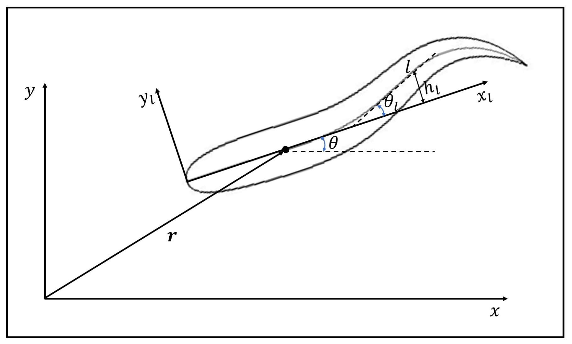
The motion of the fish body includes three parts: the body undulation in the local coordinate system (represented by the mid-line lateral displacement in – system), the translation of the mass center (), and the body rotation around the mass center (represented by the orientation angle ). The undulatory motion can be taken as the superposition of different waves propagating from head to tail. Usually the waveform is sinusoidal-based, the draw of which is that the undulating parameters cannot be smoothly changed online. Therefore, a polynomial-based undulation is adopted to allow smooth change of the waveform. In order to implement the DRL in an easy way as explained later, the kinematics of the newest generated waves can be changed every half cycle. In the n-th half cycle, the mid-line lateral displacement is determined by
where is the deflection angle of the mid-line with respect to axis , as shown in Figure 1, is the wavelength, is the period, t is the time, for and for , and h is the waveform function described by
where can be determined by , , , , and . is the maximum deflection angle at the tail tip of the n-th half wave.
2.2. Immersed Boundary-Lattice Boltzmann Method
The lattice Boltzmann method (LBM) is a numerical method used to simulate the fluid dynamics. Instead of solving the Navier–Stokes equations, the LBM solves the discrete lattice Boltzmann equation, which governs the kinematics of the mesoscopic particles,
where f is the particle density distribution function, is the space coordinate, is the discrete lattice velocity, is the time step, is the collision operator, and is the source term representing the body force. A detailed description of this equation can be found in Reference [33]. f in the whole flow field can be acquired from a well-defined boundary condition, such as the no-slip velocity condition on the boundary of the swimmer model. Once f is known, the macroscopic physical quantity such as fluid density, pressure and velocity can be computed from
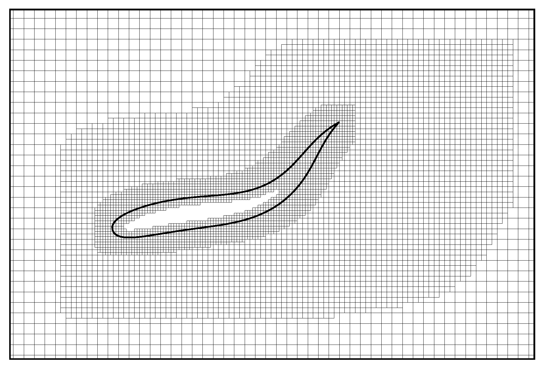
where is the lattice speed of sound in the fluid, and is the body force. Then the force and torque on the swimmer model can be computed from those macroscopic physical quantities. In addition, a diffusion immersed boundary method (IBM) [34,35,36] is utilized to handle the boundary condition at the fluid-structure interface. In this method, the influence of the boundary on the fluid is represented by a distribution of body force on the background Eulerian mesh nodes. Compared to body conformal methods [37,38,39], the grid generation in IBM is much easier for complicated shapes [35,40,41]. A multi-block geometry-adaptive Cartesian mesh (Figure 2) is coupled with the IB–LBM to accelerate the computation. A detailed description of this numerical scheme and its validation can be found in References [30,34,42,43,44,45].
2.3. Deep Reinforcement Learning
DRL is a machine learning method combining reinforcement learning with an artificial neural network. DRL has gained extensive attention due to its success in complex real-world problems [46]. In this study, a specific DRL method called deep recurrent Q-network (DRQN) [47] is adopted, in which a long-short-term-memory recurrent neural network (LSTM-RNN) is used to process time-sequential data. In this method, a smart agent learns to achieve a specific goal by interacting with its environment [23]. The agent can sense the state of the environment (denoted by s) and take actions (denoted by a) to affect it. In addition, the agent will receive a reward (denoted by ) for each action indicating how good the action is. The core idea is that the agent tries different actions in different states and finds a policy (denoted by , describing the probability of selecting each action in the different states) that maximizes the long-term reward.
The interaction procedure between the environment (IB-LBM) and the agent (DRL) is shown in Figure 3. The interaction is divided into a sequence of discrete steps . At steps n, the agents detect state , and select action , based on policy . Then the environment is changed under the influence of the action. At step , in response to the change of the environment, the agent receives reward , and finds itself in a new state . A detailed explanation of the procedure can be found in References [30,48]. Validations of the current solver can be found in Reference [30] for the hybrid method of DRL and IB-LBM.
3. Results and Discussion
3.1. Learning to Maintain a Given Speed and Orientation
In this section, a fish is trained to maintain its swimming speed and orientation to a given value. Its body length is L and its waving period is T. The goal is to swim along the x-axis at a constant average speed . The goal is reflected by defining a reward as
where is the reward of the swimmer, and and are the swimmer’s average speeds along x-axis and y-axis, respectively. In addition, the position of the leader is restricted to a confined area of .
A comprehensive representation of the environment state is very important for accurate motion control. Theoretically, it should include the information of the fish itself and the ambient flow. The information of the fish includes the body kinematic parameters, position, orientation, velocity, angular velocity, acceleration and angular acceleration of the body. The flow information includes the flow velocity and pressure in the whole flow field. In addition, the historical evolution of the flow should also be considered. The information is too complicated to be considered in a simple definition of the state. Therefore, we have conducted tests with different environment information [30]. The results show that only considering the actions, orientations, and velocities in the last four periods is enough to capture the flow dynamics and can realize relatively high accurate motion control. Therefore, the state is defined by a tuple
The swimmer propels itself by periodically generating a traveling wave propagating from head to tail, as defined by Equations (2) and (3). The period is T and the body wavelength is fixed at . The amplitude set is defined as , , , , , , , and . This parameter set forms an action base of nine components.
The simulation is performed for a Reynolds number of . Considering the desired forward swimming speed , this is equivalent to for a steady swimmer. It should be noted that this is not a typical Reynolds number for an adult fish, rather it is representative of a juvenile fish less than 5 cm in length. This Reynolds number is used to reduce the computational cost by considering laminar flow, while still demonstrating the effectiveness of the control method. The computational domain of is divided into eight layers of the block with about initial points. The minimum nondimensional mesh spacing is near the inner boundaries, and the nondimensional time step size is . The learning rate is .
The learning process is divided into a series of episodes. In each episode, the leader is initially placed in the right boundary of the confined swimming area with the initial orientation angle varying between and . The positions and orientations of the swimmer are then determined by the FSI with the actions. Once the swimmers exceed the confined area, the episode ends and another starts. Figure 4 shows the change history of the speed u and orientation angle of the swimmer when the fish starts with different initial orientations after learning for 1000 episodes. In all cases, the fish successfully aligns itself with the x-axis and remains its average swimming speed close to .
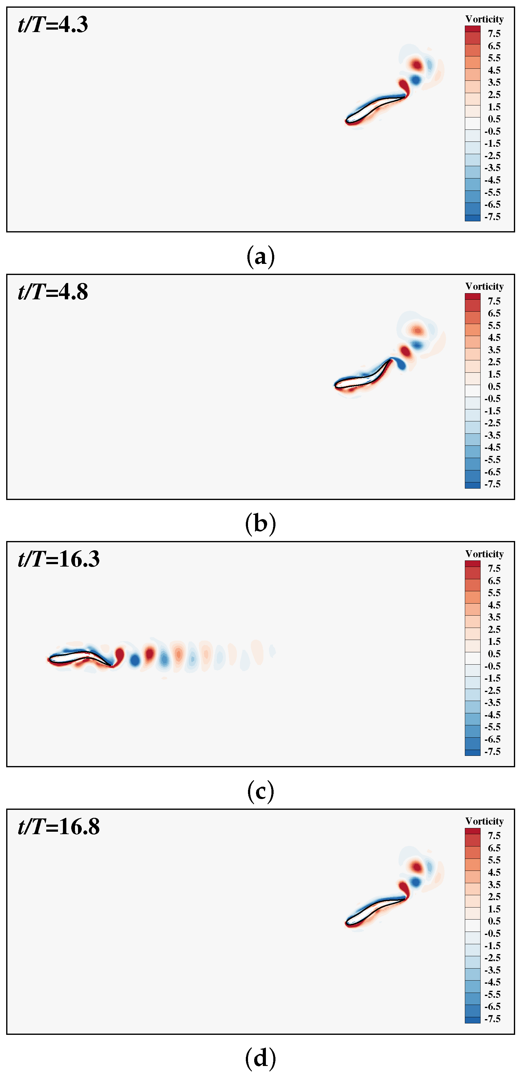
Figure 5 shows the change history of the lateral displacement of the tail tip when the fish starts with an initial orientation angle . Figure 6 shows the gestures of the fish and the vorticity contours at different instants. As can be seen, the fish adopts a higher-right-amplitude flapping to turn clockwise to align with the x-axis. Then it adopts a symmetric and constant-amplitude flapping to maintain its orientation and speed. It is noted that asymmetric corrective movement is adopted occasionally.
3.2. The Collective Motion of Two Smart Swimmers
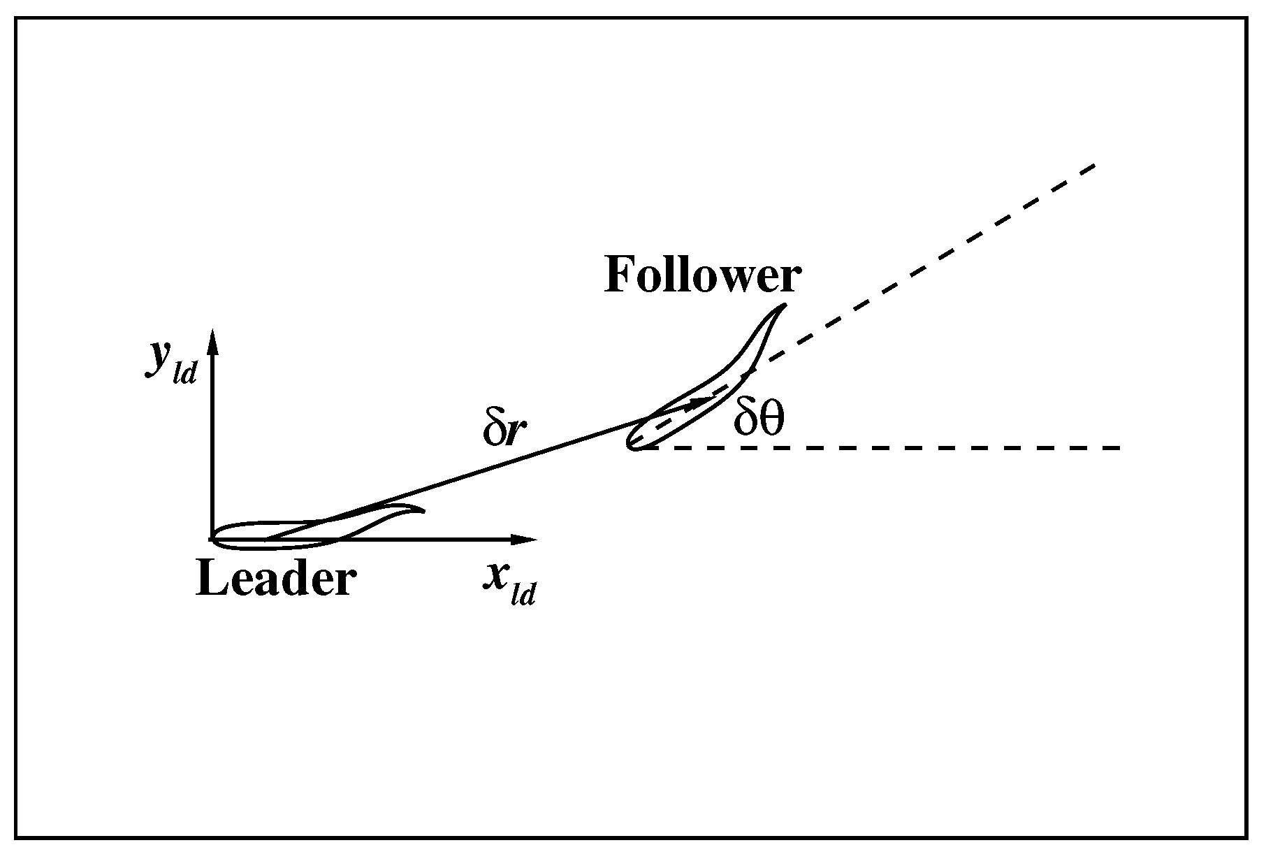
In the last section, a swimmer learns a robust control policy to maintain its swimming speed and orientation. The logic of the control policy is simple: (1) if the fish is not swimming in the desired orientation, asymmetric flapping is used to turn into the desired orientation; (2) if the fish is in the desired orientation, appropriate symmetric flapping is used to achieve the desired speed and maintain the orientation. Theoretically, if two swimmers adopt the same control policy, it would be easier for them to swim together. Therefore, in this section, the collective motion of two identical smart swimmers with the same control policy is tested in the confined swimming area. As shown in Figure 7, a leader and a follower is identified, and the relative position and orientation of the follower with respect to the leader in the local coordinate system of the leader () are represented by , and .
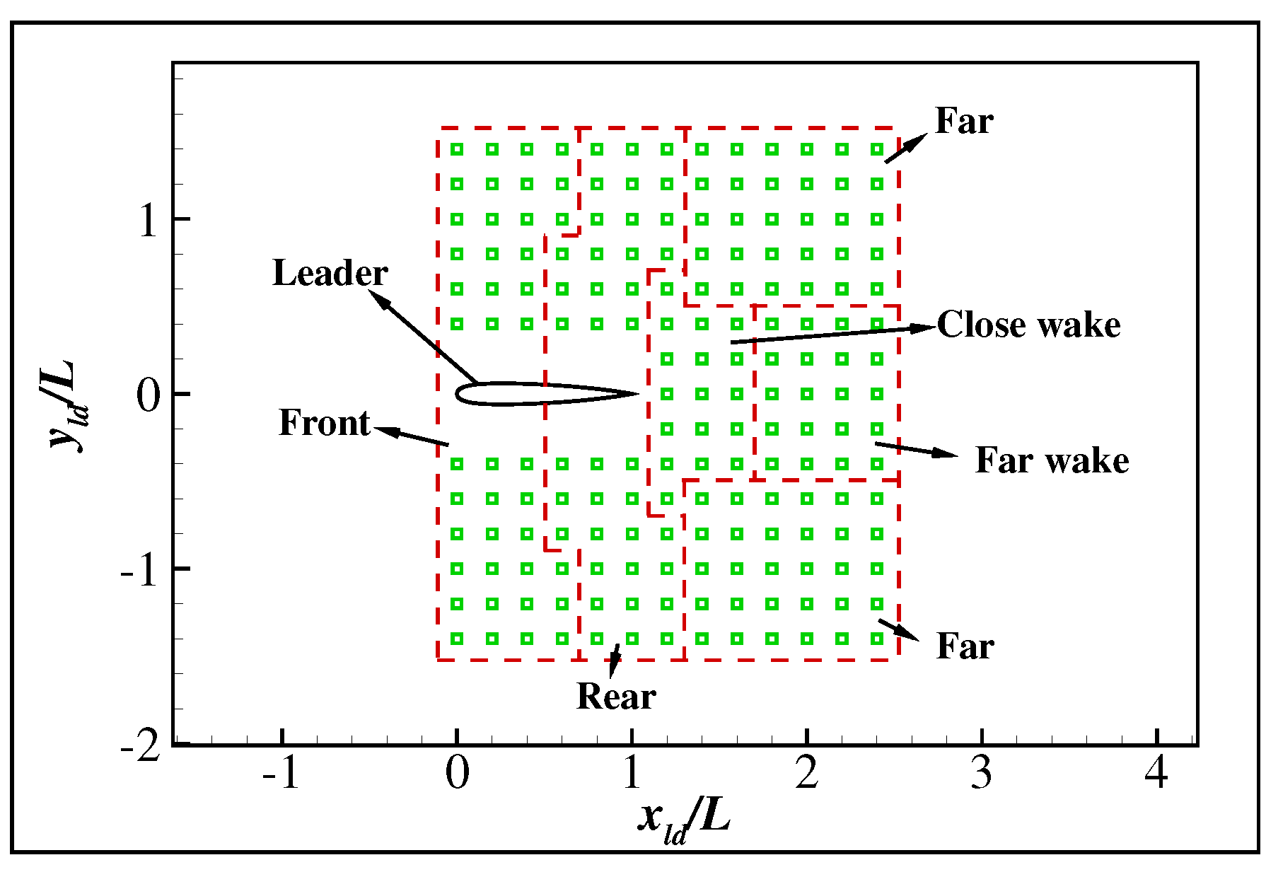
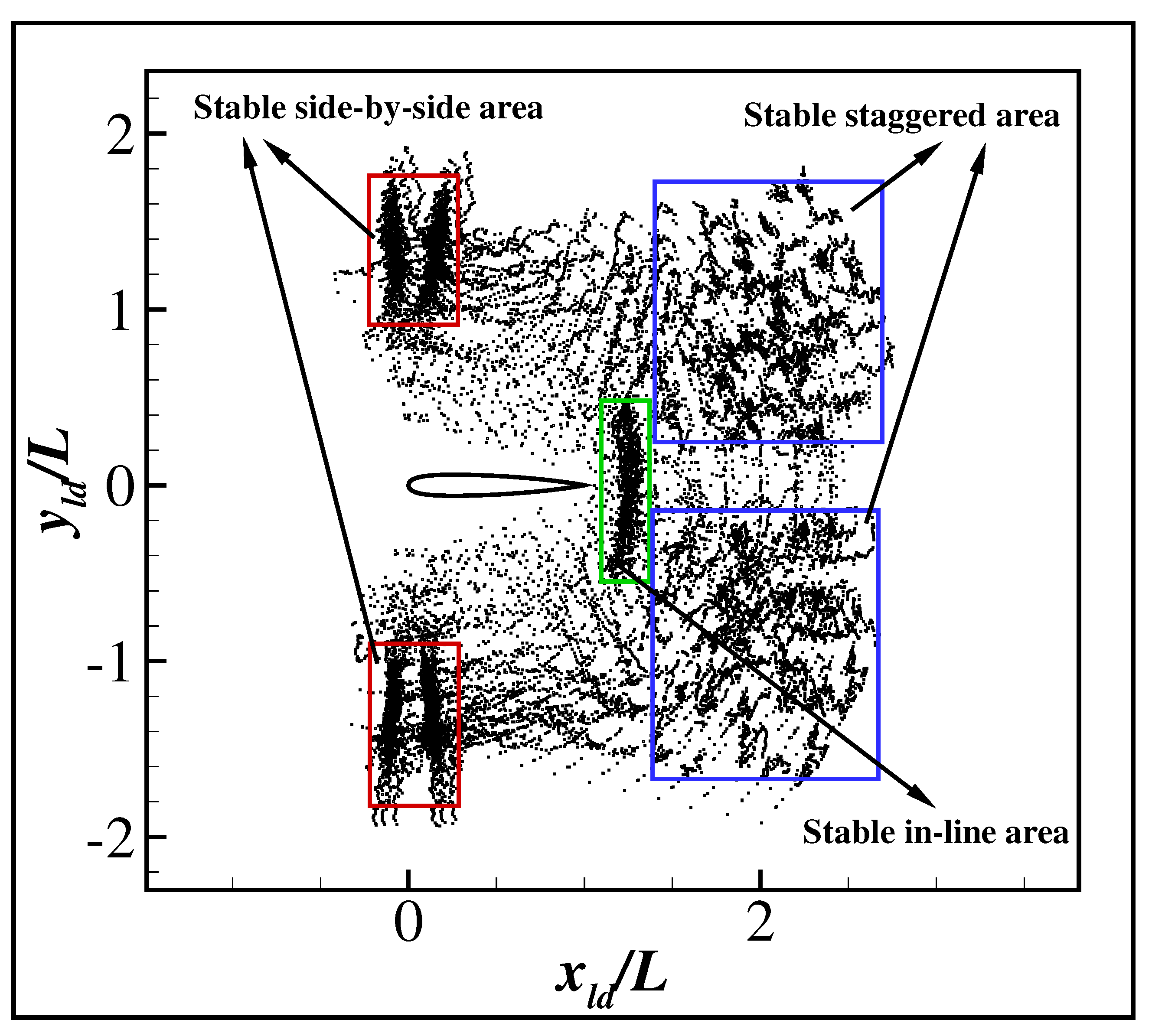
A total of 177 different cases are tested in which the initial relative orientation and the initial relative positions are as shown in Figure 8. In all cases, the swimmers drive their body according to the policy learned in the above section. The relative positions of the swimmers recorded every half a period are shown in Figure 9. The result shows that different stable formations are achieved according to the initial relative position, as shown in Figure 9. For simplicity, the flow field around the leader is divided into five different areas: front, rear, close wake, far wake and far area, as shown in Figure 8. If the initial relative position is in the front or rear area, the swimmers will form stable side-by-side swimming. If the initial relative position is in the close wake area, the swimmers will form stable in-line swimming. If the initial relative position is in the far or far wake area, the swimmers will form stable staggered swimming. The stable staggered swimming area is located in the far area, and highly diverse formations arise according to the initial formations. We noted that this is because the swimmers can easily maintain their original formations when the hydrodynamic interaction between the swimmers is negligible. The stable side-by-side area is located in a small area left or right to the leader with a distance of about . The stable in-line area is located in a small area about behind the leader. It is to be noticed that the emergence of the stable side-by-side and in-line formations from the highly diverse initial formations is due to the passive self-organization of hydrodynamics, since the swimmers always tend to maintain a given formation instead of actively alter it. In order to understand the hydrodynamic mechanism underlying the passive self-organization, three typical cases are studied in detail.
In the first case, the initial relative position is chosen as and . The relative trace of the head tip recorded every half a period is shown in Figure 10a, and the change history of the swimming speed, orientation angle and the lateral movement of the tail tip are, respectively, shown in Figure 10b–d. As can be seen, the follower is firstly behind the leader. However, it accelerates rapidly and exceeds the leader in a few periods. Then the leader catches up with the follower gradually until they swim side-by-side in a stable formation. Meanwhile, the orientation angles of both swimmers grow quickly at the beginning and then gradually restore to the initial situation.
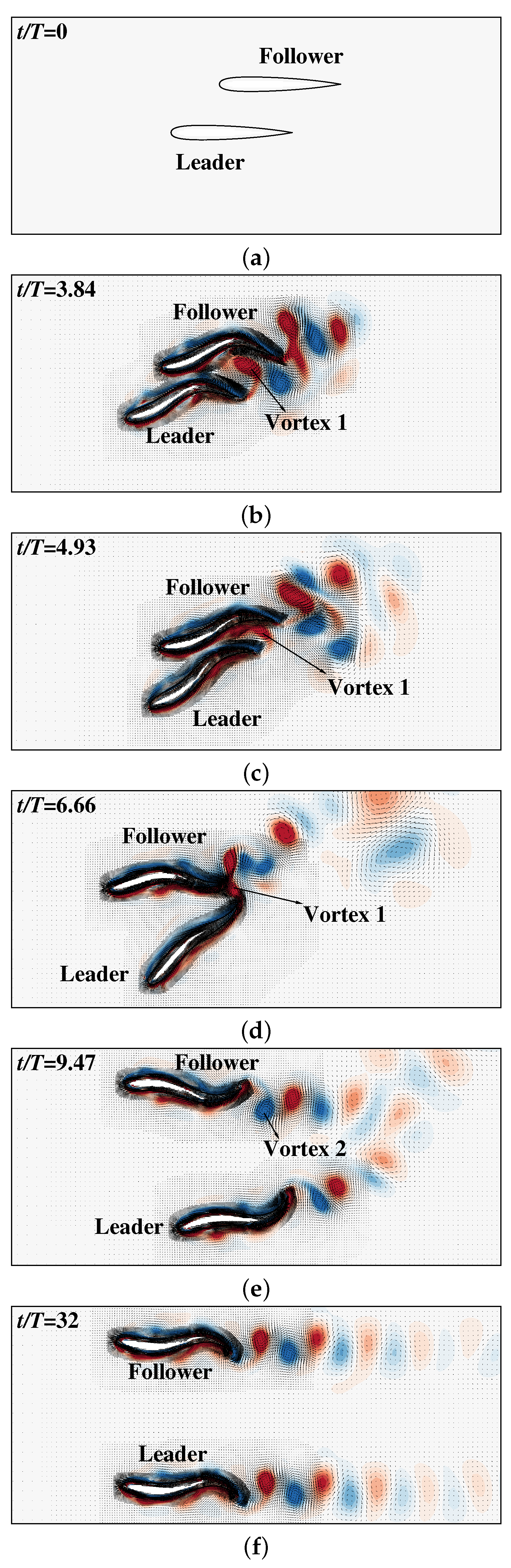
The gestures of the swimmers and the flow velocity and vorticity contours are shown in Figure 11. As can be seen, at the first few periods (Figure 11b,c), Vortex 1 (for simplicity, the newest generated counterclockwise vortex is called Vortex 1) has a strong influence on the posterior part of the leader and the middle part of the follower, making them rotating counterclockwise ( becomes larger). In addition, the vortex triggers forward flow near the follower and backward flow near the leader, which significantly accelerates the follower and decelerates the leader, as shown in Figure 10b. A few periods later (Figure 11d), the follower is very close to the leader and Vortex 1 between the swimmers exerts strong attraction force to the posterior part of them, leading to the counterclockwise rotation of the leader and the clockwise rotation of the follower. These rotations cause the swimmers to move in different directions. It is noted that this process is irreversible, which means that the swimmers will continuously swim in different directions and eventually separate (see the videos of the swimmers without active control in the Supplementary Materials). In other words, the passive mechanism does not support stable 3-DoF side-by-side swimming. This highlights the importance of active control in maintaining the stable side-by-side swimming. However, in this case, the smart swimmers are able to adjust their orientations actively. As shown in Figure 10c,d, the swimmers adopt highly asymmetric flapping to restore their orientations when the swimmers are deviated from their original orientations. Due to those active adjustments, the swimmers gradually restore their orientations and move parallel to each other, as shown in Figure 11e,f. It is to be noticed that in Figure 11e, the follower has exceeded the leader. Meanwhile, Vortex 2 instead of Vortex 1 becomes the most influential vortex, gradually accelerating the leader until the swimmers move parallel to each other. It is noted that this is a passive balance mechanism since the swimmers do not actively chase each other.
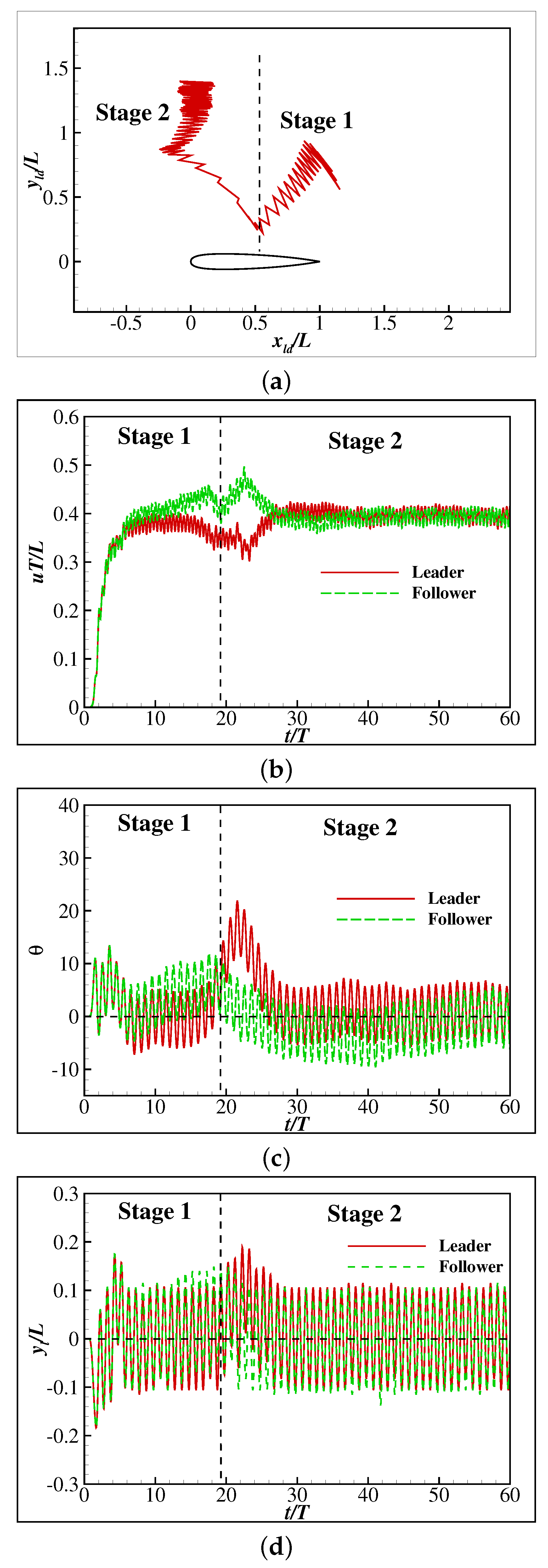
In the second case, the initial relative position is chosen as and . The relative trace of the head tip recorded every half a period is shown in Figure 12a, and the change history of the swimming speed, orientation angle and the lateral movement of the tail tip are, respectively, shown in Figure 12b–d. As can be seen, the relative motion of the follower can be divided into two stages. In Stage 1, the follower swims towards the middle part of the leader. In Stage 2, the follower swims away until it reaches the stable side-by-side position as in the first case. Considering the relative position in Stage 2 is close to that in the first case, the underlying mechanism is also similar. Therefore, the performance of the swimmers in Stage 2 is no longer discussed here. The follower is initially located parallel to the tail tip of the leader. However, it swims towards the leader with higher speed and reaches the middle part of the leader at the end of Stage 1. Meanwhile, the orientation angles of both swimmers grow gradually. Compared to the first case, the growth of the orientation angles is much smaller especially for the leader. In fact, the leader is rotating slower than the follower in this case, leading to the follower directly facing the leader.
The gestures of the swimmers and the flow velocity and vorticity contours are shown in Figure 13. As can be seen, Vortex 1 has a strong influence on the anterior part of the follower, making it rotate counterclockwise ( becomes larger) to face the leader. The vortex also triggers forward flow near the follower, which accelerates it gradually. It is noticed that the influence on the leader is much smaller than in the first case and in Stage 2. This is because the distance between the swimmers is relatively large, thus weakening the hydrodynamic interaction. In addition, this motion could lead to the collision of the swimmers (see the video in the Supplementary Materials). However, the collision is avoided in this case because the swimmers continuously adjust their flapping to resist the rotations and restore their original orientations (parallel to the x-axis). As can be seen in Figure 12d, frequent asymmetric flapping is adopted by the swimmers to parallelize the orientations. Due to these adjustments, the follower enters the front area of the leader before running into it. Thereafter, the mechanism described in the first case automatically separates the swimmers and leads them to stable side-by-side swimming.
It should also be noticed that the fishes take more than 30 periods to completely restore the speed and orientation, while in the single-fish case it takes less than 10 periods. It means that the control policy learned by the fish is not strong enough to quickly restore the speed and orientation in the presence of the hydrodynamic interaction between the fish. It can be speculated that if a more intense active adjustment strategy is utilized, the swimmers can better counteract the influence of hydrodynamic forces and restore their speeds and orientations more quickly. This mild adjustment strategy highlights the passive interaction of the fishes and thus is a good way to investigate the passive hydrodynamic mechanism of the schooling.
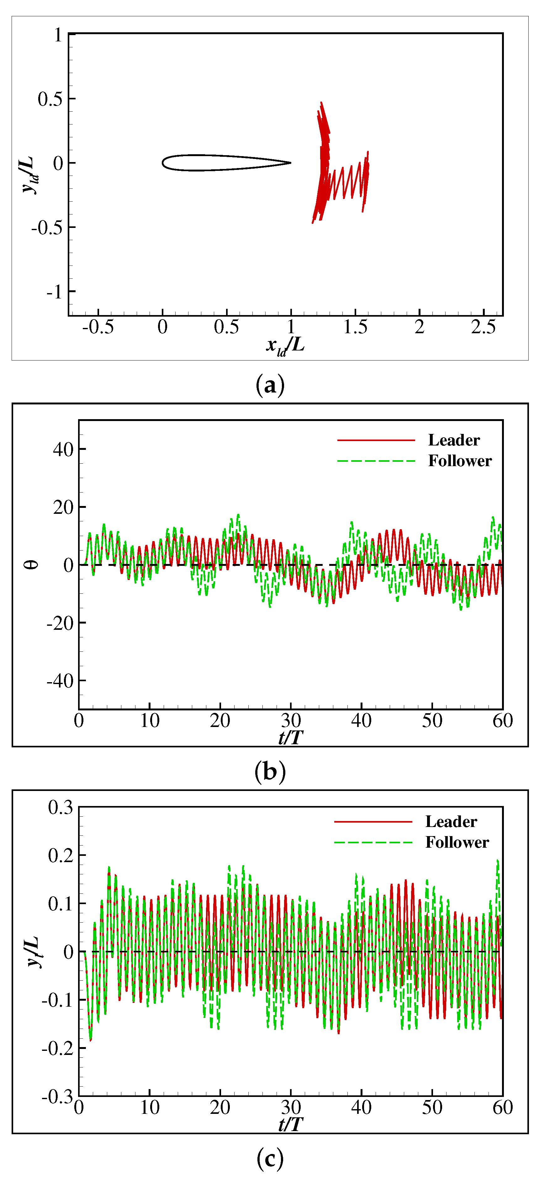
In the third case, the initial relative position is chosen as and . The relative trace of the head tip recorded every half a period is shown in Figure 14a, and the change history of the orientation angle and the lateral movement of the tail tip are, respectively, shown in Figure 14b,c. As can be seen, the follower is drawn to the leader and oscillates around the tail tip of it. Meanwhile, the orientation angles of both swimmers vary frequently, leading to the frequent adjustment movement of the swimmers.
The gestures of the swimmers and the flow velocity and vorticity contours are shown in Figure 15. Two different situations can be identified. The first situation is when the follower is in direct contact with the leader’s wake vortices, as shown in Figure 15b,c. As can be seen, the vortices are pushed to one or the other side of the follower, forming vortex pairs. The vortex pairs strengthen the lateral wake flow along a particular direction, thus push the follower out of the wake area. The second situation is when the follower is out of the wake vortices, as shown in Figure 15d. As can be seen, the vortices no longer form vortex pairs, and Vortex 1 alone has a strong influence on the follower. This is similar to Stage 1 of the second case. As is discussed, the follower should be drawn to the tail. However, since the distance between the swimmers is larger, the follower is only drawn back to the first situation where it is in direct contact with the wake flow. It is noted that this is a passive balance mechanism relying on the strength of the vortices. If the follower is located in the far wake area where the vortices are vastly weakened, it cannot be pulled back to the wake flow by the vortices and eventually swims out of the wake flow.
4. Conclusions
The collective motion of two freely-swimming smart swimmers has been numerically studied by a hybrid method of the deep reinforcement learning method (DRL) and the immersed boundary-lattice Boltzmann method (IB-LBM). An active control policy is developed by training a fish to swim in a specific speed and orientation. After training, the fish is able to restore the desired swimming speed and orientation from moderate external perturbation.
Then the control policy is adopted by two identical swimmers in the collective swimming. Results show that stable side-by-side, in-line and staggered formations are achieved according to the initial positions. The stable staggered formation is diverse since the hydrodynamic interaction between the swimmers is negligible. The stable side-by-side area is concentrated at a small area left or right to the leader with an average distance of about . The stable in-line area is concentrated in a small area about behind the leader.
In the side-by-side swimming, the follower will gradually catch up with the leader until it enters the stable side-by-side area. A detailed analysis shows that both the active control and passive self-organization play an important role in this process. The active control works for maintaining the speed and orientation of the swimmers in case they collide or depart from each other. The passive self-organization works for emerging a stable schooling configuration. This result also shows that the side-by-side swimming is 2-DoF stable even though it is 3-DoF unstable. It means that less control effort is required for the fish to remain in the side-by-side formation since it only needs to actively adjust its orientation, and the relative position will be automatically decided by the self-organization.
In the in-line swimming, the follower is drawn to the close wake area of the leader. A passive balance mechanism is identified, in which the wake vortices periodically pull the follower out of and into the wake flow. However, the stable in-line swimming only exists in specific relative positions as the mechanism relies on the ability of the vortices to draw back the follower. We noted that if an active control could serve to pull back the follower to the wake flow, more stable formations can be acquired.
This research promotes our understanding of the hydrodynamic mechanism underlying the fish schooling, especially how the active control and passive self-organization combine to form stable schooling configurations. However, as a preliminary work, many important features of the real fish swimming are not considered, making it difficult to draw a direct conclusion about the real fish behavior. Ongoing work aims to make the simulation more realistic by introducing more real fish features. To be specific, the following aspects will be explored in the future: (1) the multi-agent deep reinforcement learning will be introduced to develop a more robust and subtle control policy, in which the fishes learn to respond to not only their own environmental states but also the actions of other individuals; (2) a structure solver will be considered to reveal the active and passive energy harvesting mechanism; (3) control based on the lateral line system (using hydrodynamic information as sensory input) will be covered; and (4) three-dimensional models will be investigated. Compared to the two-dimensional cases, more degrees of freedom need to be dealt with, including the translation and rotation in three different directions. In addition, the coordinate control of the tail and the pectoral and dorsal fins should also be considered in order to balance the three-dimensional forces and torques.
Supplementary Materials
The following are available online at https://www.mdpi.com/article/10.3390/fluids7010041/s1, Video S1: single smart swimmer with initial orientation angle ; Video S2: single smart swimmer with initial orientation angle ; Video S3: first case in Section 3.2 with active control—two smart side-by-side swimmers with initial relative orientation angle and initial relative position ; Video S4: first case in Section 3.2 without active control—two free swimmers with initial relative orientation angle and initial relative position ; Video S5: second case in Section 3.2 with active control—two smart side-by-side swimmers with initial relative orientation angle and initial relative position ; Video S6: second case in Section 3.2 without active control—two free swimmers with initial relative orientation angle and initial relative position ; Video S7: third case in Section 3.2 with active control—two smart in-line swimmers with initial relative orientation angle and initial relative position ; Video S8: third case in Section 3.2 without active control—two free swimmers with initial relative orientation angle and initial relative position .
Author Contributions
Y.Z. has made contributions to the methodology, software development, data analysis and interpolation, and writing of the work. F.-B.T. has made contributions to the conception of the work, methodology, and revising of the work. J.-H.P. has made contributions to the conception and revising of the work. All authors have read and agreed to the published version of the manuscript.
Funding
Y.Z. acknowledges the Shenzhen Institute of Guangdong Ocean University and Dalian Maritime University during the pursuit of this study. This work was partially supported by the Australian Research Council (project number DE160101098).
Institutional Review Board Statement
Not applicable.
Informed Consent Statement
Not applicable.
Data Availability Statement
Raw data are available upon request.
Conflicts of Interest
The authors declare no conflict of interest.
Abbreviations
The following abbreviations are used in this manuscript:
| DoF | degree of freedom |
| DRL | deep reinforcement learning |
| IB-LBM | immersed boundary-lattice Boltzmann method |
| FSI | fluid–structure interaction |
| IBM | immersed boundary method |
| LBM | lattice Boltzmann method |
| DRQN | deep recurrent Q-network |
| LSTM-RNN | long-short-term-memory recurrent neural network |
References
- Larsson, M. Why do fish school? Curr. Zool. 2012, 58, 116–128. [Google Scholar] [CrossRef] [Green Version]
- Brown, G.E.; Godin, J.G.J. Anti-predator responses to conspecific and heterospecific skin extracts by threespine sticklebacks: Alarm pheromones revisited. Behaviour 1997, 134, 1123–1134. [Google Scholar] [CrossRef]
- Pitcher, T.; Magurran, A.; Winfield, I. Fish in larger shoals find food faster. Behav. Ecol. Sociobiol. 1982, 10, 149–151. [Google Scholar] [CrossRef]
- Pitcher, T.J. Functions of shoaling behaviour in teleosts. In The Behaviour of Teleost Fishes; Springer: Berlin/Heidelberg, Germany, 1986; pp. 294–337. [Google Scholar]
- Weihs, D. Hydromechanics of fish schooling. Nature 1973, 241, 290–291. [Google Scholar] [CrossRef]
- Lighthill, S.J. Mathematical Biofluiddynamics; Society for Industrial and Applied Mathematics SIAM: Philadelphia, PA, USA, 1975. [Google Scholar]
- Deng, J.; Shao, X.M.; Yu, Z.S. Hydrodynamic studies on two traveling wavy foils in tandem arrangement. Phys. Fluids 2007, 19, 113104. [Google Scholar] [CrossRef]
- Boschitsch, B.M.; Dewey, P.A.; Smits, A.J. Propulsive performance of unsteady tandem hydrofoils in an in-line configuration. Phys. Fluids 2014, 26, 051901. [Google Scholar] [CrossRef]
- Ashraf, I.; Godoy-Diana, R.; Halloy, J.; Collignon, B.; Thiria, B. Synchronization and collective swimming patterns in fish (Hemigrammus bleheri). J. R. Soc. Interface 2016, 13, 20160734. [Google Scholar] [CrossRef] [PubMed] [Green Version]
- Tian, F.B.; Wang, W.; Wu, J.; Sui, Y. Swimming performance and vorticity structures of a mother–calf pair of fish. Comput. Fluids 2016, 124, 1–11. [Google Scholar] [CrossRef]
- Kurt, M.; Moored, K. Unsteady Performance of Finite-Span Pitching Propulsors in Side-by-Side Arrangements. In Proceedings of the 2018 Fluid Dynamics Conference, Atlanta, GA, USA, 24 June 2018; p. 3732. [Google Scholar]
- Ramananarivo, S.; Fang, F.; Oza, A.; Zhang, J.; Ristroph, L. Flow interactions lead to orderly formations of flapping wings in forward flight. Phys. Rev. Fluids 2016, 1, 071201. [Google Scholar] [CrossRef]
- Zhu, X.; He, G.; Zhang, X. Flow-mediated interactions between two self-propelled flapping filaments in tandem configuration. Phys. Rev. Lett. 2014, 113, 238105. [Google Scholar] [CrossRef]
- Dai, L.; He, G.; Zhang, X.; Zhang, X. Stable formations of self-propelled fish-like swimmers induced by hydrodynamic interactions. J. R. Soc. Interface 2018, 15, 20180490. [Google Scholar] [CrossRef] [PubMed]
- Park, S.G.; Sung, H.J. Hydrodynamics of flexible fins propelled in tandem, diagonal, triangular and diamond configurations. J. Fluid Mech. 2018, 840, 154–189. [Google Scholar] [CrossRef]
- Kurt, M.; Mivehchi, A.; Moored, K.W. Two-dimensionally stable self-organization arises in simple schooling swimmers through hydrodynamic interactions. arXiv 2021, arXiv:2102.03571. [Google Scholar]
- Novati, G.; Verma, S.; Alexeev, D.; Rossinelli, D.; Van Rees, W.M.; Koumoutsakos, P. Synchronisation through learning for two self-propelled swimmers. Bioinspir. Biomim. 2017, 12, 036001. [Google Scholar] [CrossRef] [PubMed] [Green Version]
- Bergmann, M.; Iollo, A. Modeling and simulation of fish-like swimming. J. Comput. Phys. 2011, 230, 329–348. [Google Scholar] [CrossRef]
- Gazzola, M.; Hejazialhosseini, B.; Koumoutsakos, P. Reinforcement learning and wavelet adapted vortex methods for simulations of self-propelled swimmers. SIAM J. Sci. Comput. 2014, 36, B622–B639. [Google Scholar] [CrossRef] [Green Version]
- Yan, L.; Chang, X.; Tian, R.; Wang, N.; Zhang, L.; Liu, W. A numerical simulation method for bionic fish self-propelled swimming under control based on deep reinforcement learning. Proc. Inst. Mech. Eng. Part C J. Mech. Eng. Sci. 2020, 234, 3397–3415. [Google Scholar] [CrossRef]
- Gazzola, M.; Tchieu, A.A.; Alexeev, D.; de Brauer, A.; Koumoutsakos, P. Learning to school in the presence of hydrodynamic interactions. J. Fluid Mech. 2016, 789, 726–749. [Google Scholar] [CrossRef] [Green Version]
- Verma, S.; Novati, G.; Koumoutsakos, P. Efficient collective swimming by harnessing vortices through deep reinforcement learning. Proc. Natl. Acad. Sci. USA 2018, 115, 5849–5854. [Google Scholar] [CrossRef] [Green Version]
- Colabrese, S.; Gustavsson, K.; Celani, A.; Biferale, L. Flow navigation by smart microswimmers via reinforcement learning. Phys. Rev. Lett. 2017, 118, 158004. [Google Scholar] [CrossRef] [Green Version]
- Colabrese, S.; Gustavsson, K.; Celani, A.; Biferale, L. Smart inertial particles. Phys. Rev. Fluids 2018, 3, 084301. [Google Scholar] [CrossRef] [Green Version]
- Biferale, L.; Bonaccorso, F.; Buzzicotti, M.; Clark Di Leoni, P.; Gustavsson, K. Zermelo’s problem: Optimal point-to-point navigation in 2D turbulent flows using reinforcement learning. Chaos Interdiscip. J. Nonlinear Sci. 2019, 29, 103138. [Google Scholar] [CrossRef] [PubMed]
- Jiao, Y.; Ling, F.; Heydari, S.; Kanso, E.; Heess, N.; Merel, J. Learning to swim in potential flow. Phys. Rev. Fluids 2021, 6, 050505. [Google Scholar] [CrossRef]
- Alageshan, J.K.; Verma, A.K.; Bec, J.; Pandit, R. Machine learning strategies for path-planning microswimmers in turbulent flows. Phys. Rev. E 2020, 101, 043110. [Google Scholar] [CrossRef] [PubMed]
- Tsang, A.C.H.; Tong, P.W.; Nallan, S.; Pak, O.S. Self-learning how to swim at low Reynolds number. Phys. Rev. Fluids 2020, 5, 074101. [Google Scholar] [CrossRef]
- Daddi-Moussa-Ider, A.; Löwen, H.; Liebchen, B. Hydrodynamics can determine the optimal route for microswimmer navigation. Commun. Phys. 2021, 4, 1–11. [Google Scholar]
- Zhu, Y.; Tian, F.B.; Young, J.; Liao, J.C.; Lai, J.C. A numerical study of fish adaption behaviors in complex environments with a deep reinforcement learning and immersed boundary-lattice Boltzmann method. Sci. Rep. 2021, 11, 1–20. [Google Scholar]
- Tian, F.B. A numerical study of linear and nonlinear kinematic models in fish swimming with the DSD/SST method. Comput. Mech. 2015, 55, 469–477. [Google Scholar] [CrossRef]
- Zhou, C.; Shu, C. Simulation of self-propelled anguilliform swimming by local domain-free discretization method. Int. J. Numer. Methods Fluids 2012, 69, 1891–1906. [Google Scholar] [CrossRef]
- Krüger, T.; Kusumaatmaja, H.; Kuzmin, A.; Shardt, O.; Silva, G.; Viggen, E.M. The Lattice Boltzmann Method; Springer: Berlin/Heidelberg, Germany, 2017. [Google Scholar]
- Ma, J.; Wang, Z.; Young, J.; Lai, J.C.; Sui, Y.; Tian, F.B. An immersed boundary-lattice Boltzmann method for fluid-structure interaction problems involving viscoelastic fluids and complex geometries. J. Comput. Phys. 2020, 415, 109487. [Google Scholar] [CrossRef]
- Huang, W.X.; Tian, F.B. Recent trends and progress in the immersed Boundary method. Proc. Inst. Mech. Eng. Part C J. Mech. Eng. Sci. 2019, 233, 7617–7636. [Google Scholar] [CrossRef]
- Xu, Y.Q.; Tang, X.Y.; Tian, F.B.; Peng, Y.H.; Xu, Y.; Zeng, Y.J. IB–LBM simulation of the haemocyte dynamics in a stenotic capillary. Comput. Methods Biomech. Biomed. Eng. 2014, 17, 978–985. [Google Scholar]
- Tian, F.B.; Bharti, R.P.; Xu, Y.Q. Deforming-Spatial-Domain/Stabilized Space–Time (DSD/SST) method in computation of non-Newtonian fluid flow and heat transfer with moving boundaries. Comput. Mech. 2014, 53, 257–271. [Google Scholar] [CrossRef]
- Tian, F.B. FSI modeling with the DSD/SST method for the fluid and finite difference method for the structure. Comput. Mech. 2014, 54, 581–589. [Google Scholar] [CrossRef]
- Tian, F.B.; Wang, Y.; Young, J.; Lai, J.C. An FSI solution technique based on the DSD/SST method and its applications. Math. Model. Methods Appl. Sci. 2015, 25, 2257–2285. [Google Scholar] [CrossRef]
- Mittal, R.; Iaccarino, G. Immersed boundary methods. Annu. Rev. Fluid Mech. 2005, 37, 239–261. [Google Scholar] [CrossRef] [Green Version]
- Sotiropoulos, F.; Yang, X. Immersed boundary methods for simulating fluid–structure interaction. Prog. Aerosp. Sci. 2014, 65, 1–21. [Google Scholar] [CrossRef]
- Xu, L.; Tian, F.B.; Young, J.; Lai, J.C. A novel geometry-adaptive Cartesian grid based immersed boundary-lattice Boltzmann method for fluid–structure interactions at moderate and high Reynolds numbers. J. Comput. Phys. 2018, 375, 22–56. [Google Scholar] [CrossRef]
- Xu, L.; Wang, L.; Tian, F.B.; Young, J.; Lai, J.C. A geometry-adaptive immersed boundary-lattice Boltzmann method for modelling fluid–structure interaction problems. In IUTAM Symposium on Recent Advances in Moving Boundary Problems in Mechanics; Springer: Berlin/Heidelberg, Germany, 2019; pp. 161–171. [Google Scholar]
- Young, J.; Tian, F.B.; Liu, Z.; Lai, J.C.; Nadim, N.; Lucey, A.D. Analysis of unsteady flow effects on the Betz limit for flapping foil power generation. J. Fluid Mech. 2020, 902, A30. [Google Scholar] [CrossRef]
- Tian, F.B.; Luo, H.; Zhu, L.; Liao, J.C.; Lu, X.Y. An efficient immersed boundary-lattice Boltzmann method for the hydrodynamic interaction of elastic filaments. J. Comput. Phys. 2011, 230, 7266–7283. [Google Scholar] [CrossRef] [PubMed] [Green Version]
- Mnih, V.; Kavukcuoglu, K.; Silver, D.; Rusu, A.A.; Veness, J.; Bellemare, M.G.; Graves, A.; Riedmiller, M.; Fidjeland, A.K.; Ostrovski, G. Human-level control through deep reinforcement learning. Nature 2015, 518, 529. [Google Scholar] [CrossRef] [PubMed]
- Hausknecht, M.; Stone, P. Deep Recurrent Q-Learning for Partially Observable MDPs. In Proceedings of the 2015 AAAI Fall Symposium Series, Ithaca, NY, USA, 27 August 2015. [Google Scholar]
- Tampuu, A.; Matiisen, T.; Kodelja, D.; Kuzovkin, I.; Korjus, K.; Aru, J.; Aru, J.; Vicente, R. Multiagent cooperation and competition with deep reinforcement learning. PLoS ONE 2017, 12, e0172395. [Google Scholar] [CrossRef]
Figure 1.
A schematic illustration of the motion of the fish.

Figure 2.
Near-boundary grid structure of a fish-like body.

Figure 3.
The interaction procedure between IB-LBM and DRL.

Figure 4.
Single smart swimmer: (a) The change history of the speed for different initial orientation angles; and (b) the change history of the orientation angle for different initial orientation angles.
Figure 4.
Single smart swimmer: (a) The change history of the speed for different initial orientation angles; and (b) the change history of the orientation angle for different initial orientation angles.

Figure 5.
The lateral movement of the tail of a single smart swimmer with an initial orientation angle .
Figure 5.
The lateral movement of the tail of a single smart swimmer with an initial orientation angle .

Figure 6.
Vorticity contours behind a single smart swimmer at four typical instants: (a) , (b) , (c) , (d) . The range of the vorticity contours is from to . Note that the flow inside the body-occupied region is introduced by the IB-LBM, which however does not affect the solution in the physical region.

Figure 7.
A schematic illustration of the relative position of the swimmers.

Figure 8.
The initial relative positions of the follower in different test cases.

Figure 9.
The traces of the follower in the local coordinate system of the leader in different test cases.
Figure 9.
The traces of the follower in the local coordinate system of the leader in different test cases.

Figure 10.
Collective swimming starts in front area: (a) The trace of the head tip, (b) the change of the speed, (c) the change of the orientation angle, (d) the lateral movement of the tail tip.
Figure 10.
Collective swimming starts in front area: (a) The trace of the head tip, (b) the change of the speed, (c) the change of the orientation angle, (d) the lateral movement of the tail tip.

Figure 11.
Vorticity contours behind the fish during side-by-side swimming initiated in the front area at six typical instants: (a) , (b) , (c) , (d) , (e) , and (f) . The range of the vorticity contours is from to .
Figure 11.
Vorticity contours behind the fish during side-by-side swimming initiated in the front area at six typical instants: (a) , (b) , (c) , (d) , (e) , and (f) . The range of the vorticity contours is from to .

Figure 12.
Collective swimming starts in the rear area: (a) The trace of the head tip, (b) the change of the speed, (c) the change of the orientation angle, (d) the lateral movement of the tail tip.
Figure 12.
Collective swimming starts in the rear area: (a) The trace of the head tip, (b) the change of the speed, (c) the change of the orientation angle, (d) the lateral movement of the tail tip.

Figure 13.
Vorticity contours behind the fish during side-by-side swimming initiated in the rear area at four typical instants in Stage 1: (a) , (b) , (c) , (d) . The range of the vorticity contours is from to .
Figure 13.
Vorticity contours behind the fish during side-by-side swimming initiated in the rear area at four typical instants in Stage 1: (a) , (b) , (c) , (d) . The range of the vorticity contours is from to .

Figure 14.
Collective swimming starts in close wake area: (a) The trace of the head tip, (b) the change of the orientation angle, (c) the lateral movement of the tail tip.
Figure 14.
Collective swimming starts in close wake area: (a) The trace of the head tip, (b) the change of the orientation angle, (c) the lateral movement of the tail tip.

Figure 15.
Vorticity contours behind the fish during in-line swimming at four typical instants: (a) , (b) , (c) , (d) . The range of the vorticity contours is from to .
Figure 15.
Vorticity contours behind the fish during in-line swimming at four typical instants: (a) , (b) , (c) , (d) . The range of the vorticity contours is from to .

Publisher’s Note: MDPI stays neutral with regard to jurisdictional claims in published maps and institutional affiliations. |
© 2022 by the authors. Licensee MDPI, Basel, Switzerland. This article is an open access article distributed under the terms and conditions of the Creative Commons Attribution (CC BY) license (https://creativecommons.org/licenses/by/4.0/).
Share and Cite
MDPI and ACS Style
Zhu, Y.; Pang, J.-H.; Tian, F.-B. Stable Schooling Formations Emerge from the Combined Effect of the Active Control and Passive Self-Organization. Fluids 2022, 7, 41. https://doi.org/10.3390/fluids7010041
AMA Style
Zhu Y, Pang J-H, Tian F-B. Stable Schooling Formations Emerge from the Combined Effect of the Active Control and Passive Self-Organization. Fluids. 2022; 7(1):41. https://doi.org/10.3390/fluids7010041
Chicago/Turabian StyleZhu, Yi, Jian-Hua Pang, and Fang-Bao Tian. 2022. "Stable Schooling Formations Emerge from the Combined Effect of the Active Control and Passive Self-Organization" Fluids 7, no. 1: 41. https://doi.org/10.3390/fluids7010041