
Optimal Design of Bacterial Carpets for Fluid Pumping


1
Department of Mathematics and BioInspired Syracuse, Syracuse University, 900 South Crouse Avenue, Syracuse, NY 13244, USA
2
Department of Mathematics, Syracuse University, 900 South Crouse Avenue, Syracuse, NY 13244, USA
3
Department of Mathematics, University of San Diego, 5998 Alcalá Park, San Diego, CA 92110, USA
4
Department of Mathematics and Statistics, James Madison University, 800 South Main Street, Harrisonburg, VA 22807, USA
5
Department of Mathematics, Applied Mathematics and Statistics, Case Western Reserve University, 10090 Euclid Avenue, Cleveland, OH 44106, USA
*
Author to whom correspondence should be addressed.
†
These authors contributed equally to this work.
Fluids 2022, 7(1), 25; https://doi.org/10.3390/fluids7010025
Submission received: 6 October 2021
/
Revised: 11 December 2021
/
Accepted: 29 December 2021
/
Published: 5 January 2022
(This article belongs to the Special Issue 20 Years of Regularized Stokeslets: Applications, Computation, and Theory)
Abstract
:In this work, we outline a methodology for determining optimal helical flagella placement and phase shift that maximize fluid pumping through a rectangular flow meter above a simulated bacterial carpet. This method uses a Genetic Algorithm (GA) combined with a gradient-based method, the Broyden-Fletcher-Goldfarb-Shanno (BFGS) algorithm, to solve the optimization problem and the Method of Regularized Stokeslets (MRS) to simulate the fluid flow. This method is able to produce placements and phase shifts for small carpets and could be adapted for implementation in larger carpets and various fluid tasks. Our results show that given identical helices, optimal pumping configurations are influenced by the size of the flow meter. We also show that intuitive designs, such as uniform placement, do not always lead to a high-performance carpet.
1. Introduction
Bacterial carpets consist of multiple flagellated bacteria naturally or artificially adhered to a surface, with the flagella positioned outward into the fluid. The geometry of the surrounding fluid may be open [1] or it may be inside a tube or microscale channel [2]. The study of fluid flow or pumping by bacterial carpets has been of significant interest in microfluidics for the past couple of decades. There are numerous experimental studies on flow and mixing induced by helices [3,4,5], biomimetic cilia [6,7], and bacterial carpets [1,2,8,9,10].
These carpets can be modeled using various numerical representations of flagella by rigid or flexible helices. Because of the small length scales involved, these fluids are often modeled as low-Reynolds-number, Newtonian fluids [11]. Additionally, a number of numerical studies have been performed to examine the effect of these carpets on mixing and pumping [12,13,14,15]. Several of these studies have observed that helical placement and phase shifts alter the qualitative and quantitative characteristics of the fluid flow. However, to the best of the authors’ knowledge, no existing work has systematically looked at optimizing flow subject to these helical parameters.
Ideally these bacterial carpets are created in order to control or achieve either a directional flow or mixing in the fluid. In this study, the authors outline an approach to maximize the volume of fluid pumped through a flow meter placed slightly above the simulated helices subject to several variables such as the locations of the helices and their phase shifts. Such an optimization problem faces the following two fundamental challenges. First, a priori knowledge of what makes a carpet ‘good’ at pumping is lacking. Second, function evaluations for the objective task (pumping) are computationally costly fluid simulations. We seek a method that strikes a balance between reliability in finding the optimal carpet and computational efficiency.
The fluid simulations outlined in Section 2.1, Section 2.2 and Section 2.3 are based on those from [12,13] for simulating fluid flows induced by one or more rigid helical structures rotating with each helix attached to a wall (semi-infinite domain). Section 2.4 outlines a method which first employs a genetic algorithm [16,17,18] applied to a surrogate model in order to obtain a good starting guess for an optimal carpet. Compared to the full model, the surrogate model can be simulated at a substantially reduced computational cost. This carpet is then used as the initial solution in a gradient-based method [19,20,21,22,23,24,25] to find the optimal carpet. Our method takes advantage of the genetic algorithm’s ability to perform a global search along with the efficiency and accuracy of the gradient-based method. The procedure outlined here addresses optimizing the flow subject to helical parameters and has broad utility as a framework which may be adapted for a multitude of future applications. This method is tested and validated in Section 3 for cases of one, two, three, and four helices.
2. Methods
We model a bacterial carpet as a collection of rigid, helical filaments attached to a stationary planar wall and immersed in a viscous fluid. In Section 2.1, we lay out the Method of Regularized Stokeslets (MRS) used to solve the fluid equations. Section 2.2 and Section 2.3 describe the setup of both the rigid helices and the flow meter developed and utilized as a measure for the optimization described in Section 2.4.
2.1. Fluid Solver
The methods described in this section are pulled directly from [12,13]. The fluid is governed by the incompressible Stokes equations
where is fluid pressure, is fluid viscosity, is fluid velocity, and is an external force density acting on the fluid. Using the MRS [26,27], we characterize the external force at each point as a smooth concentrated force . Here, is a constant vector and is a smooth approximation of the Dirac delta function commonly referred to as a blob function. In this work,
The forces acting on the fluid come from the N points discretizing the rigid bodies in the fluid. Note that the MRS calculates the exact solution due to a regularized point force. To model a helical filament with nonzero effective thickness, we distribute regularized point forces along its centerline. Implementing the MRS, the velocity at any point resulting from forces located at positions is
where . Note that the forces are implemented at the positions , and the velocity can be evaluated at any point without requiring an underlying computational grid for the fluid domain, hence the velocity is defined everywhere.
When evaluating the velocity at the positions , Equation (3) can be written as
where A is , is and contains the N velocities , and is and contains the N forces . To prescribe the kinematics of the rigid, rotating helices, one must define the velocities at the N points on the helices and solve the linear system (4) for the N forces that result in the desired velocity. These forces can then be used in Equation (3) to find the resulting velocity at any point in the unbounded domain. In practice, we solve a non-dimensional system, as is shown in detail in [12].
To incorporate a stationary planar wall, the method of images for regularized Stokeslets [28] is used to enforce a no-slip boundary condition. In this formulation, an image source consisting of a regularized Stokeslet, doublet, dipole, and rotlet is mirrored across the boundary. This results in an infinite planar wall at which the velocity is zero, and no underlying grid is required to model the wall. In previous work [13], it was shown that the choice of boundary condition affects the efficiency of a bacterial carpet at pumping fluid. Therefore, we expect that when a different boundary condition is considered, such as the periodic boundary condition [29,30], the optimal configuration of the carpet will change. In terms of implementation, the optimization methods described in Section 2.4 still apply; the only change is how the objective function of the optimization problem (see Section 2.3) should be evaluated. (To be more precise, using a different boundary condition only affects how the flow field is calculated within the objective function.)
2.2. Helical Flagellum
As in previous work [12,13], we model each bacterial flagellum as a rotating helical filament, , whose centerline, parametrized by , is
for . Here, L is the height of the helix, is the helical radius, is a tapering parameter, is the helical pitch, and is the phase shift. We then discretize each helix into n equally spaced points. As in the Refs. [13,31], we choose parameters to be close to the typical dimensions of Escherichia coli bacteria. All default parameters, given in non-dimensional units, are listed in Table 1.
The kinematics of each helix are prescribed using the time-dependent rotation matrix
with angular velocity . A negative value of results in a clockwise rotation when viewed from above. At any point in time, the position of the helix is given by
where is the location of the base point.
In this work, the helices are assumed to be rigid. Under this assumption, we can prescribe their shape and motion as above. In many biophysical problems, the shape and motion of cilia or flagella are a result of fluid-structure interactions and typically unknown a priori. Models that are more suitable for these problems can be found in [32,33], for example. Although the model described here is not realistic in some applications, such as carpets made up of live bacteria, it is appropriate for man-made carpets and allows for a straight-forward investigation into questions of optimization.
2.3. Measurement of Pumping
In order to quantify fluid pumping by a carpet of helices described in Section 2.2, we measure the volume of fluid pumped upward through a flow meter stationed above the carpet during one rotation of the helices, as in the Ref. [13].
More precisely, the flow meter is chosen to be the following square “patch” parallel to the no-slip wall at :
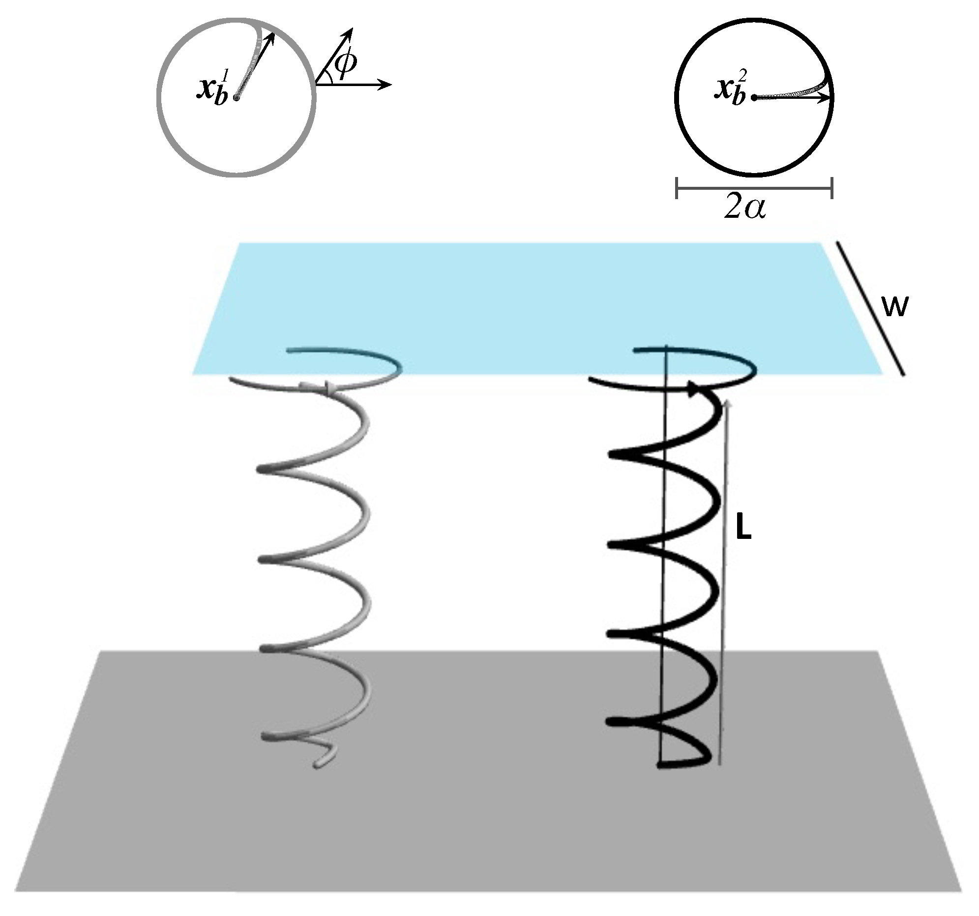
where is greater than the height L of the helices and W denotes the width of the patch. Figure 1 shows such a flow meter above a carpet consisting of two helices. We note that the only boundary of the fluid is the infinite, planar, and solid wall at , on which the flow vanishes. The flow meter simply provides a means of quantifying pumping and is not physically placed in the fluid. Thus, it has no effect on the fluid flow.
Let contain all the design parameters that we aim to optimize. As specified in Section 3, in this work, the design parameters are the coordinates of the base points and the phase shifts of the helices. Nevertheless, the methods described in this section and in Section 2.4 still apply if different design parameters are considered. The following function then quantifies pumping for a carpet whose configuration is determined by the choice of :
where T is the time that it takes for the helices to perform one rotation and denotes the z- direction fluid velocity at a point on the flow meter (7) at time t. Given , we estimate as follows. We first approximate the triple integral in Equation (8) by the following double integral:
where is the number of time steps, is the size of the time step, and for ; and then we evaluate (9) using a quadrature rule. The values of T and used in the numerical experiments can be found in Table 1. The fluid velocities at the quadrature points discretizing the flow meter (7) are calculated using the MRS.
As outlined in Section 2.1, at each time point , calculating the forces exerted by the points on the helices to the surrounding fluid requires solving a linear system (4) whose coefficient matrix is of size , where N is the number of points. The computational cost, using the standard “big ” notation, is therefore . After the forces have been calculated, evaluating at quadrature points entails additional operations (see Equation (3)). In summary, the computational complexity of evaluating is
This implies that the computational cost of evaluating increases cubically with the number of helices in the carpet, assuming that the same number of points are used to discretize each helix. The computational cost also increases with the size of the flow meter since more quadrature points are needed to approximate the integral (9) if the same accuracy is desired.
2.4. Optimization
To optimize the helical parameters of a bacterial carpet for a task (fluid pumping in the case of this work), we must solve the following optimization problem:
where contains d design parameters, such as the locations of the helices and their phase shifts, is a scalar function that measures the performance of the carpet at the task. (Depending on the task and definition of , we may wish to maximize or minimize . In this work, the goal is to maximize ). Unfortunately, an analytic form of is usually unavailable and evaluating it entails numerical simulations of the fluid around the carpet. To solve (11), we need to apply a numerical optimization algorithm, which in turn requires evaluating f at different ’s. In this section, we discuss two such algorithms: Genetic Algorithms (GAs) which are gradient-free and typically used to find a global optimizer, and the Broyden–Fletcher–Goldfarb–Shanno (BFGS) algorithm, a gradient-dependent, quasi-Newton method that can converge to a local optimizer quickly if a good estimate is given. To find a global optimizer of efficiently, we propose to use a hybrid method that exploits both a GA’s ability at identifying a global optimizer and the BFGS algorithm’s fast convergence.
2.4.1. Genetic Algorithms (GAs)
GAs [16,17,18] are often applied to find the global minimum or maximum of a function. They “evolve” a pool of candidate solutions towards better solutions through an iterative process inspired by natural selection. More specifically, the best solutions of the current generation are selected, recombined, and possibly mutated to produce the next generation of solutions. We first randomly select the initial generation of solutions. In each iteration that follows, a portion of the current generation of solutions is chosen at random to be “parents” to the next generation. The solutions that produce lower (higher) function values are more likely to be chosen, if the minimum (maximum) is sought. Two parent solutions can be combined as follows to produce a “child” solution. Every entry of the child solution is set to the corresponding entry of one of the parents, depending on the result of a coin flip. We can also mutate a parent solution to produce a child solution by adding a number taken from a Gaussian distribution with mean 0 to each entry of the parent solution. GAs return the best solution among the final generation of candidate solutions as the optimizer. We note that the methods described above are not unique, and there exist many options for the creation of the initial population and the selection, crossover, and mutation of the parent solutions. Custom methods that are tailored to the optimization problem (11) at hand can also be devised. Like natural selection, GAs are stochastic, and therefore, their performance may be affected by the sequence of random numbers used.
GAs and gradient-free optimization methods in general suffer from slow convergence. As will be shown in Section 3.1, even for the simplest carpet made up of a single helix, a GA entails thousands of evaluations of the objective function. This can be prohibitively expensive for fluid problems such as the ones considered here.
2.4.2. The Broyden-Fletcher-Goldfarb-Shanno (BFGS) Algorithm
The BFGS algorithm [21,22,23,24,25] is an iterative method for optimization that starts with an initial guess and calculates a new estimate as
where is a scalar and a search direction. Like in Newton’s method, the search direction in Equation (12) is obtained by solving a linear system
where is the gradient of f at . In Newton’s method, the coefficient matrix in Equation (13) is the Hessian matrix associated with f at , whereas the BFGS algorithm uses an approximation to the Hessian instead that is considerably easier to calculate and invert. After has been calculated, in Equation (12) is then chosen to be the scalar that optimizes . When an analytic form of is unavailable, such as in the problems considered here, the gradient needs to be approximated numerically, for example, by the forward difference method.
The BFGS algorithm converges rapidly to a local optimizer of if the initial guess is close to it. However, the algorithm may get “stuck” at a local optimizer that is not global if is not carefully chosen; unfortunately, for the problems considered here, it remains unclear how to choose it. As will be shown in Section 3, even for simple carpets, the initial configuration that we intuit may turn out to be inferior.
2.4.3. The Hybrid Method
To take advantage of both a GA’s higher reliability at finding the global optimizer and the BFGS algorithm’s higher efficiency given a good initial guess, we propose to use a hybrid approach for solving (11) that consists of the following two steps:
- Step 1:
- find a maximizer of using a GA, where s is a surrogate model for f;
- Step 2:
- find a maximizer of using the BFGS algorithm with as the initial guess for .
The surrogate model should be significantly cheaper to evaluate than so that it is feasible to apply a GA to it in Step 1, yet it should also be sufficiently representative of so that will be close to and thus the BFGS algorithm will converge quickly in Step 2. The that we use employs coarser temporal, spatial discretization and will be specified in Section 3.
3. Results
All the computational results are obtained in MATLAB® version R2017a on a virtual machine equipped with two Intel® Xeon® E7-8890 v4 Processors with twenty-four cores per processor and 64GB of RAM. MATLAB’s Parallel Computing Toolbox is used to parallelize the computations. Default parameters are given in Table 1 and do not vary throughout the numerical experiments. Using a different set of values will only affect the evaluation of the objective function and does not affect how the optimization methods described in Section 2.4 will be implemented. The design parameters are chosen to be the phase shifts and coordinates of the bases of the helices, and we aim to determine their optimal values that achieve maximal pumping using the methods in Section 2.4. We consider carpets made up of a single helix (Section 3.1), a pair of helices (Section 3.2), and multiple helices (Section 3.3).
Applying the hybrid method described in Section 2.4.3 to the optimization problem (11) entails evaluating the objective function and its surrogate repeatedly at different ’s. As shown in Table 1, the spatial and temporal discretization used in s is about ten times as coarse as the discretization used in f. For flow meters of various sizes and carpets consisting of various numbers of helices, we compare the runtimes required to evaluate and . Specifically, we consider three values of the width W of the flow meter (7): , 5, and 10 as well as cases of one, two, and four helices. The runtimes entailed by evaluating and for each combination of W and number of helices are listed in Table 2. Here, and for the rest of the paper, runtimes are measured in seconds by MATLAB’s tic and toc commands. Recall that a double integral must be evaluated to calculate or (see (9)). We use MATLAB’s function integrate2 with its default setting to approximate this integral numerically.
As seen in Table 2, the time to evaluate both and increases with the number of helices and the size of the flow meter; this is expected given the computational complexity (10). The runtime increases with the size of the flow meter because more quadrature points are needed as the domain of integration in (9) increases. For the same flow meter and number of helices, evaluating is significantly cheaper than evaluating .
3.1. A Single Helix
We first consider the case of a single helix by investigating the following question: Where should the helix be placed to maximize pumping? We fix all design parameters of the helix except for the coordinates of its base point, that is, in the optimization problem (11).
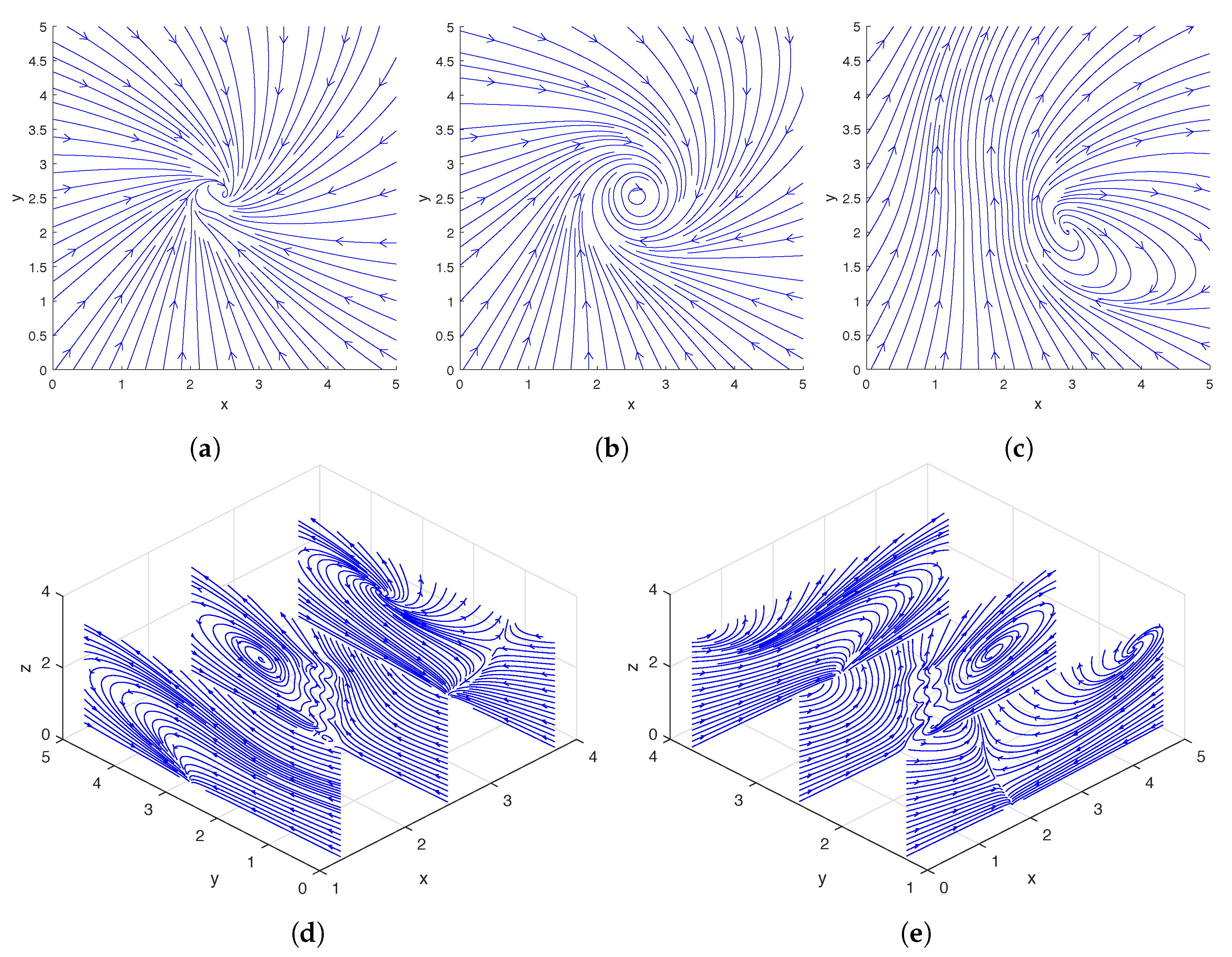
In Figure 2, we show the streamlines drawn based on the instantaneous fluid velocity around a rotating helix. As can be seen in Figure 2d,e, the helix moves the fluid near its tip upward while rotating, and there are also regions of downward flow away from the helix. A more detailed experimental analysis of the flow field around a single rotating helix can be found in [31] and a numerical study was performed in [12,13].
Since we consider an incompressible Newtonian fluid, as the width W of the flow meter (7) approaches infinity, the volume of the fluid pumped through the meter goes to zero regardless of the values of the design parameters. However, in applications, only flow meters of finite sizes are of interest, and the volume of fluid that is transported through a finite flow meter does change depending on the placement of the helix relative to the flow meter.
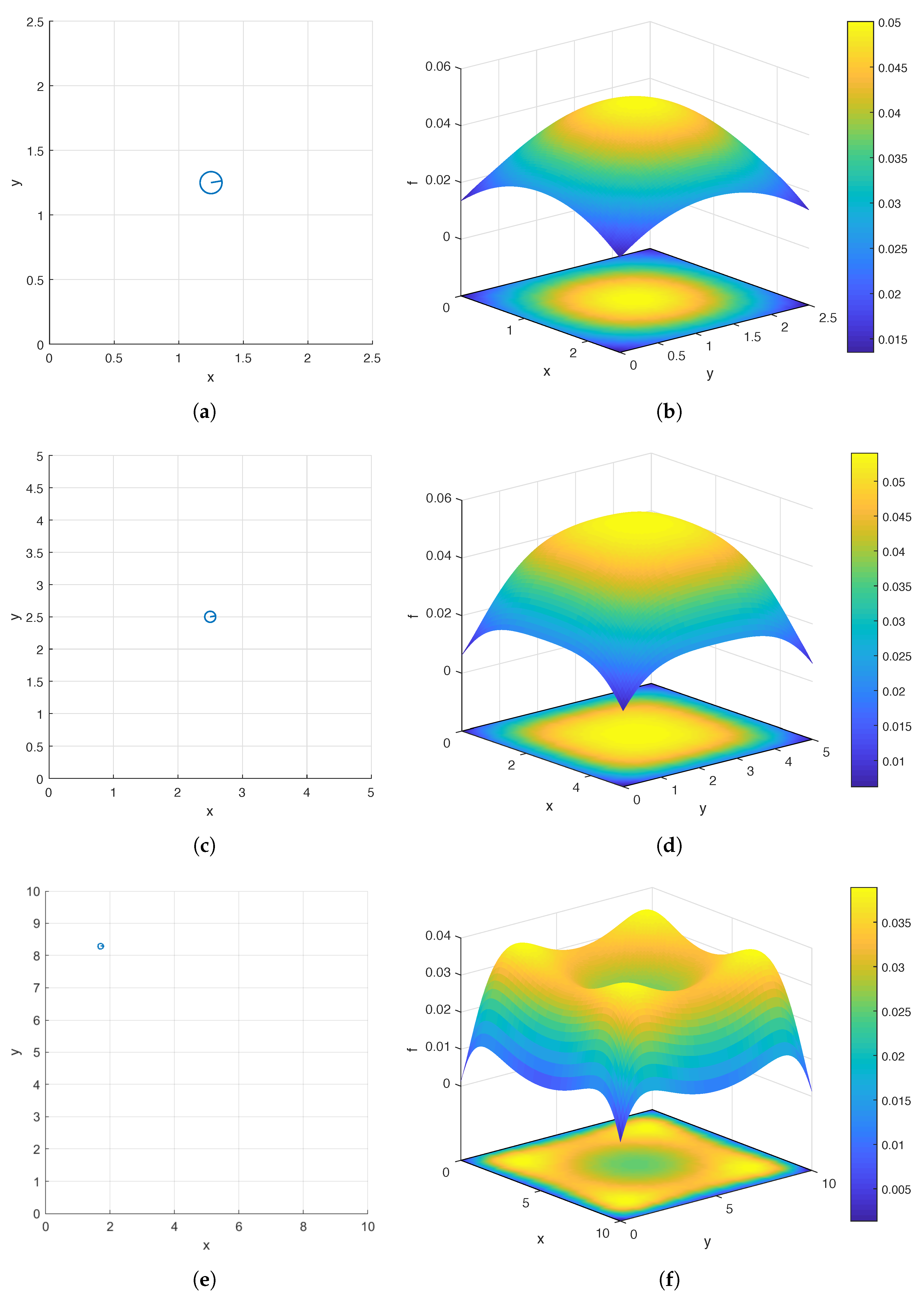
We consider a square flow meter defined by (7) and three values of W: , 5, and 10. In Figure 3b,d,f, we show the surface and contour plots of over the domain corresponding to , 5, and 10, respectively. For each W, in order to produce the pair of plots, we sample f at the following uniformly distributed grid points:
As can be seen in Figure 3b,d,f, for all three values of W, global maximizers of f lie on the diagonals of the domain. It is interesting to note that while the global maximizer is the center of the domain and unique when or 5, there are four global maximizers located near the four corners of the domain when . While intuition might lead one to expect the center to be the global maximizer, in fact, it is a local minimizer when , and the global maximum () is considerably larger than this local minimum (). This clearly demonstrates the importance of quantitative analysis when searching for an optimal design of a bacterial carpet.
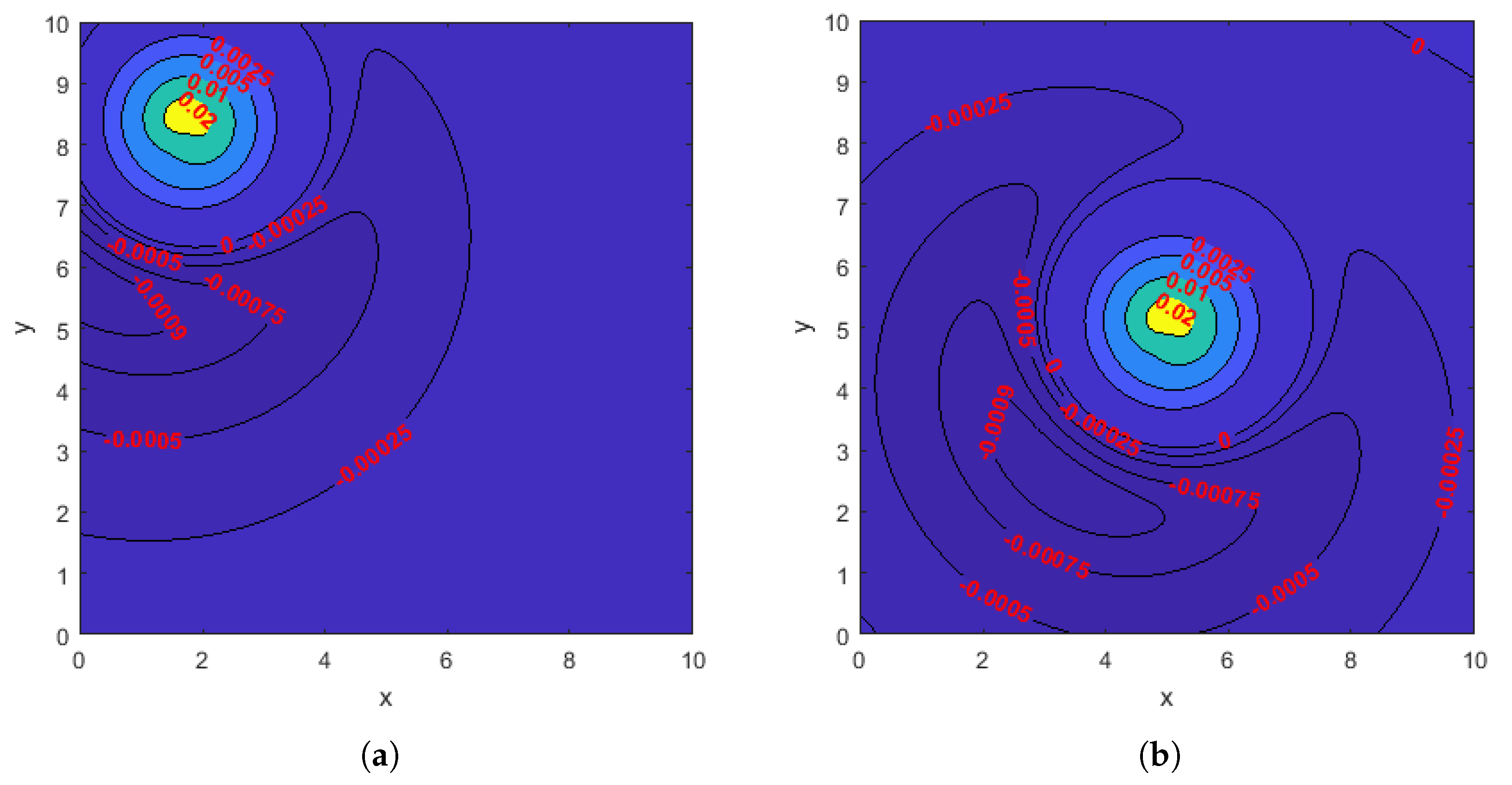
To further investigate why the optimal location of the helix is near the corners instead of the center of the domain when the width of the flow meter is 10, in Figure 4, we draw the contour plots of the instantaneous z-direction fluid velocity on the flow meter when the helix is based at one of the four optimal locations (Figure 4a) and when it is based at the center of the domain (Figure 4b). Comparing the two contour plots, we observe that when the helix is based at the center, a considerably larger region on the flow meter has small negative z-direction velocity. More precisely, the areas enclosed by the level curves corresponding to z-direction velocities , , , and in Figure 4b are almost twice as large as their counterparts in Figure 4a. In addition, Figure 4 also helps explain why the optimal location of the helix is at the center when the width of the flow meter is or 5: both flow meters are small enough that placing the helix at the center maximizes the region with large positive z-direction velocity while creating no region or only a negligible region where the z-direction velocity is negative.
We apply both the hybrid method described in Section 2.4.3 and a GA to solve (11) and compare their performance. In Step 1 of the hybrid method, we apply a GA to find a maximizer of , the surrogate model of (see Table 1 and Table 2 for a comparison of the two functions); and in Step 2 of the hybrid method, we apply the BFGS algorithm with initial guess to find a maximizer of . In Table 3, we list the maximizers and found in the hybrid method for flow meters (7) of widths , 5, and 10. In Figure 3a,c,e, we also display the top views of the optimal carpets corresponding to the three flow meters respectively. Table 4 and Table 5 contain the numbers of iterations, the numbers of function evaluations, and the runtimes of the hybrid method and a GA, respectively. We use MATLAB’s ga function, an implementation of a GA, to find maximizers for both and . The default setting of ga is used except that parallel computing is enabled and the range of the initial generation of candidate solutions is set to . We note that GAs are not deterministic (see Section 2.4.1). Thus, for reproducibility of the results presented in Table 3, Table 4 and Table 5, we reset the seed of MATLAB’s random number generators to 0 using the command rng default before calling the function ga. We use MATLAB’s fminunc function with its default setting, which implements the BFGS algorithm, to find a maximizer of in Step 2 of the hybrid method (Both MATLAB functions ga and fminunc are for the minimization of a given objective function. Since we wish to maximize or instead, in our MATLAB implementation, we use or as the objective function).
As seen in Table 4 and Table 5, for all three flow meters, the hybrid method is significantly more efficient than the GA, requiring less runtime. Although the GA requires about three thousand function evaluations to converge whether it is applied to or , since is considerably cheaper to evaluate (see Table 2), applying the GA to is also considerably cheaper. In the hybrid method, once the estimate is found by the GA in Step 1, the BFGS algorithm, which starts with , converges quickly to the maximizer in Step 2, requiring only two or three iterations and less than 20 function evaluations. Moreover, we can see that the hybrid method is more accurate than the GA by comparing the maximizers and found by the two methods, respectively (see Table 3 and Table 5). We also observe that the runtimes of both the hybrid method and GA increase with the size of the flow meter. Note that since the initial candidate solutions are randomly chosen in the GA, in the case where the flow meter is , both the hybrid method and GA may find different maximizers in different runs if we do not reset the seed of the random number generators to the same number.
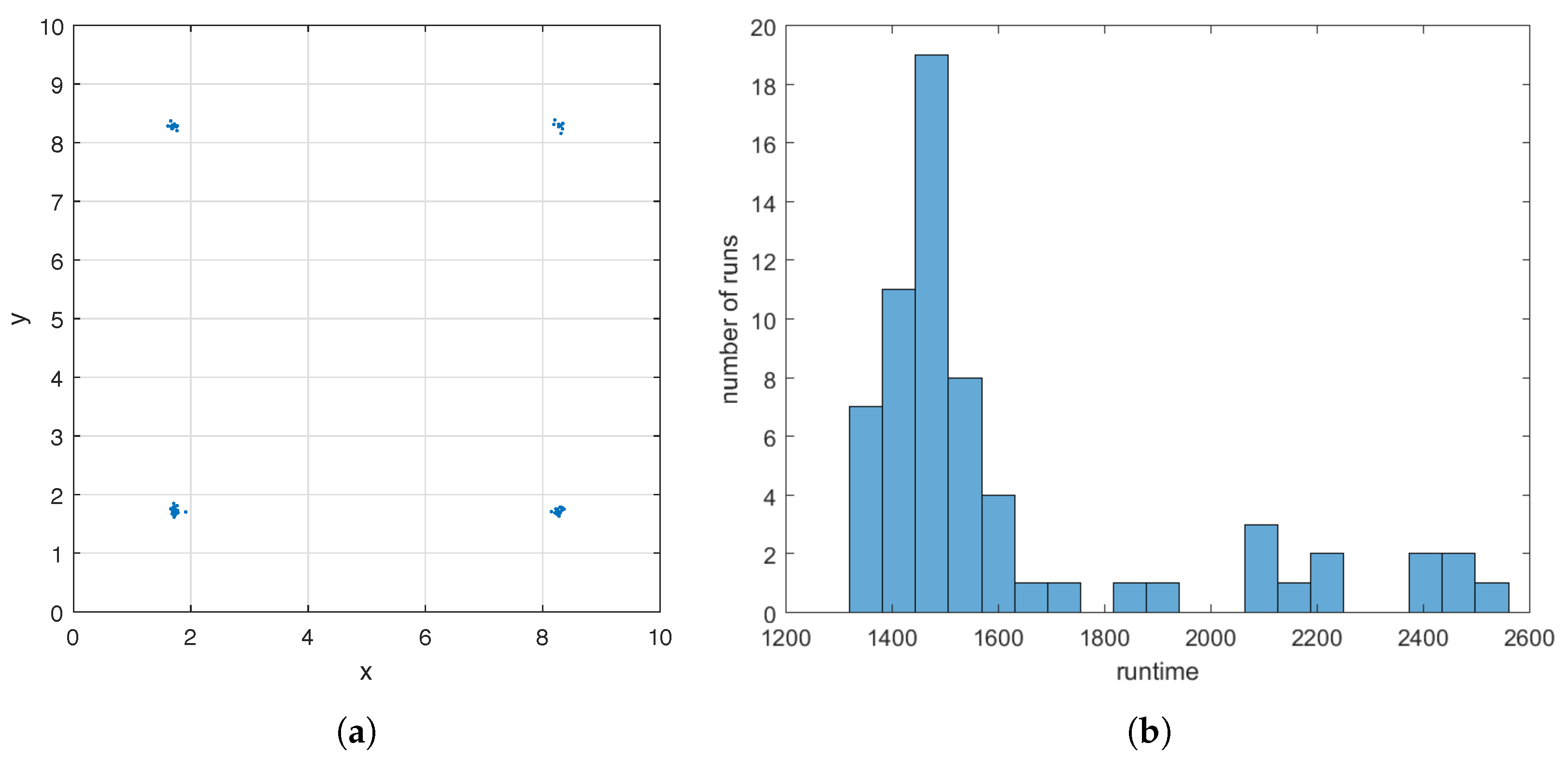
To demonstrate the robustness of the GA at finding a good initial guess in Step 1 of the hybrid method, for the case where the flow meter is , we apply the GA to sixty-four times and initialize the random number generators based on the current time using the command rng shuffle before each run. The GA uses a different sequence of random numbers in each run due to the re-initialization. In Figure 5a, we display all sixty-four ’s found by the GA. They form four clusters around the four maximizers of (see Figure 3f), and the sizes of the clusters are 20, 19, 10, and 15. This demonstrates that the GA applied to always finds an initial guess close to one of the maximizers of , although the maximizer may differ from run to run depending on the sequence of random numbers used. Runtime of the GA varies with the seed of the random number generators as well. In Figure 5b, we show a histogram of the sixty-four runtimes, the majority of which is less than 1800 s.
3.2. A Pair of Helices
We now apply the hybrid method to find an optimal design of a carpet consisting of two helices for fluid pumping. We set the phase shift of the first helix to zero () and let the design parameters be the coordinates of the base points of the two helices and the phase shift of the second helix. That is,
This optimization problem (11) is significantly more difficult to solve than the one in Section 3.1, not only because there are more design parameters (five instead of two) but also because the computational cost of evaluating and increases with the number of helices (see (10)) as is shown in Table 2.
In Figure 6, we show the streamlines drawn based on the instantaneous fluid velocity around a pair of rotating helices. As can be seen in Figure 6d,e, the helices move the fluid near their tips upward while rotating. A more detailed analysis of the flow field around a pair of rotating helices can be found in [13].
We again consider a square flow meter (7) and three values of W, as in Section 3.1. The maximizers found by the hybrid method are listed in Table 6 and the top views of the corresponding optimal carpets are displayed in Figure 7. We use to denote the maximizer of found by the GA and to denote the maximizer of found by the BFGS algorithm using as its initial guess. The iteration counts, numbers of function evaluations, and runtimes of the GA and BFGS algorithm are reported in Table 7.
As can be seen in Table 6 and Figure 7, the hybrid method suggests that in order to maximize pumping, we should place the pair of helices along the diagonal of the domain and set the phase shift of the second helix to (recall that the phase shift of the first helix is fixed at 0). These results are consistent with what was observed in [13] in that pumping was maximized when the difference between the phase shifts is . However, we note that while this does maximize pumping, the distance between the optimal locations of the helices is sufficiently large so that when they are placed at these locations, the choice of phase shifts has a minimal impact on pumping. (For a pair of helices, the effect of the difference between their phase shifts on pumping has been studied in [13], where they were placed at various distances apart.) This is similarly observed for the cases of three and four helices considered in Section 3.3. We conjecture that the choice of phase shifts will play a greater role when the optimal locations of the helices are forced to be closer to one another, such as when there are more helices or when the flow meter is smaller.
Table 7 shows that, like in the case of a single helix, although a large number of iterations and function evaluations are needed for the GA to find the initial guess, , once it is found, the BFGS algorithm only requires a relatively small number of iterations and function evaluations to converge to the maximizer, . Additionally, the total runtime of the hybrid method increases with the size of the flow meter.
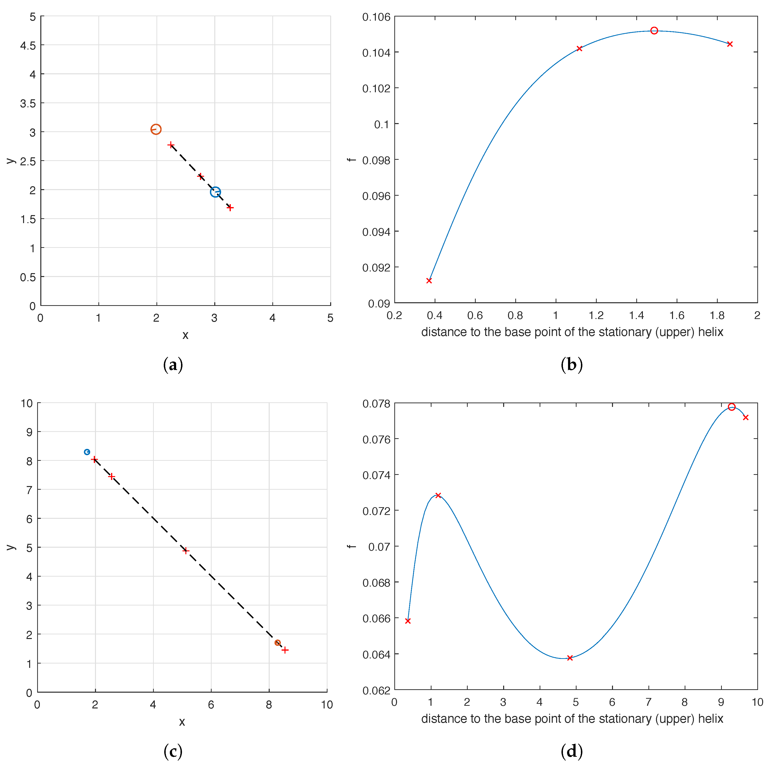
In the case with one helix, because we were optimizing over only two parameters, the coordinates of the base of the helix, we could easily visualize the objective function. Now however, we are optimizing over five parameters (the base coordinates of each helix, and the phase shift of the second) so it is more difficult to visualize our objective function in a useful way. In order to investigate how the placement of the pair of helices affects the carpet’s performance at pumping, for the flow meters (7) with widths and 10, we fix the phase shifts of both helices, the location of one of the them and calculate as the location of the other helix is varied. To be more precise, we fix all the design parameters of the optimal carpets shown in Figure 7b,c except for the location of the lower helix. We then examine the value of as we move the lower helix along the dashed line shown in Figure 8a,c. This line goes through the base points and of the two helices in the optimal carpet found by the hybrid method. As can be seen in Figure 8b, when , the pumping capability of the carpet first grows as the distance increases, peaks as the moving helix reaches its optimal position found by the hybrid method, and then starts to decline as the distance increases further. For the case , the graph of is quite similar and not shown here. As shown in Figure 8d, the graph of is even more interesting in the case of . As the distance increases, the value of first increases to reach a local maximum and then decreases to reach a local minimum, before it increases again to the global maximum when the moving helix is at its optimal position calculated by the hybrid method. In Figure 8, a few sample locations of the moving helix as well as the corresponding values of are marked for reference.
3.3. Multiple Helices
We also apply the hybrid method to determine optimal designs that maximize pumping for carpets consisting of three and four helices. The design parameters are the coordinates of the base points and phase shifts of the helices. (The phase shift of the first helix is fixed at 0, as in Section 3.2). Thus, there are eight and eleven design parameters in these two cases respectively.
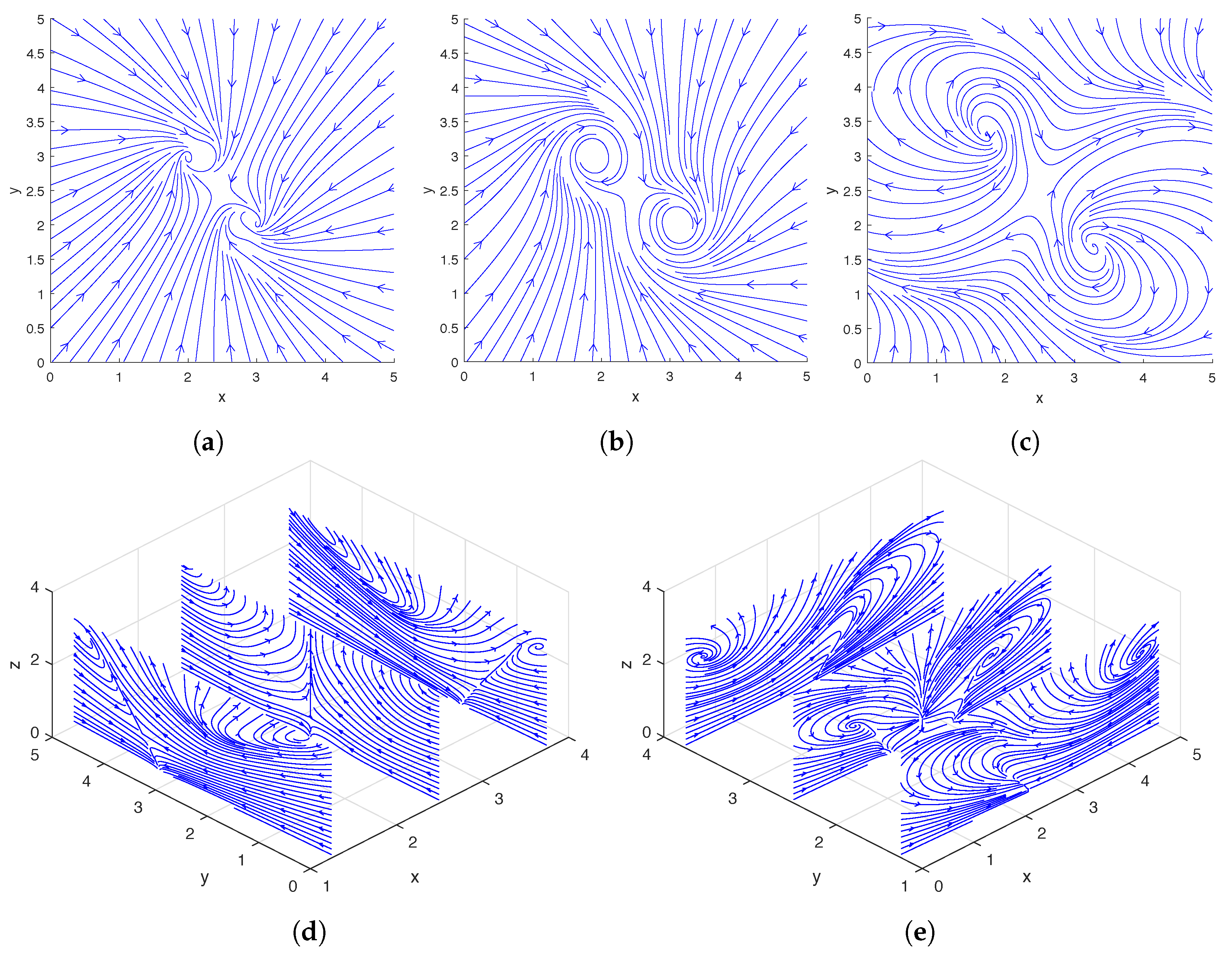
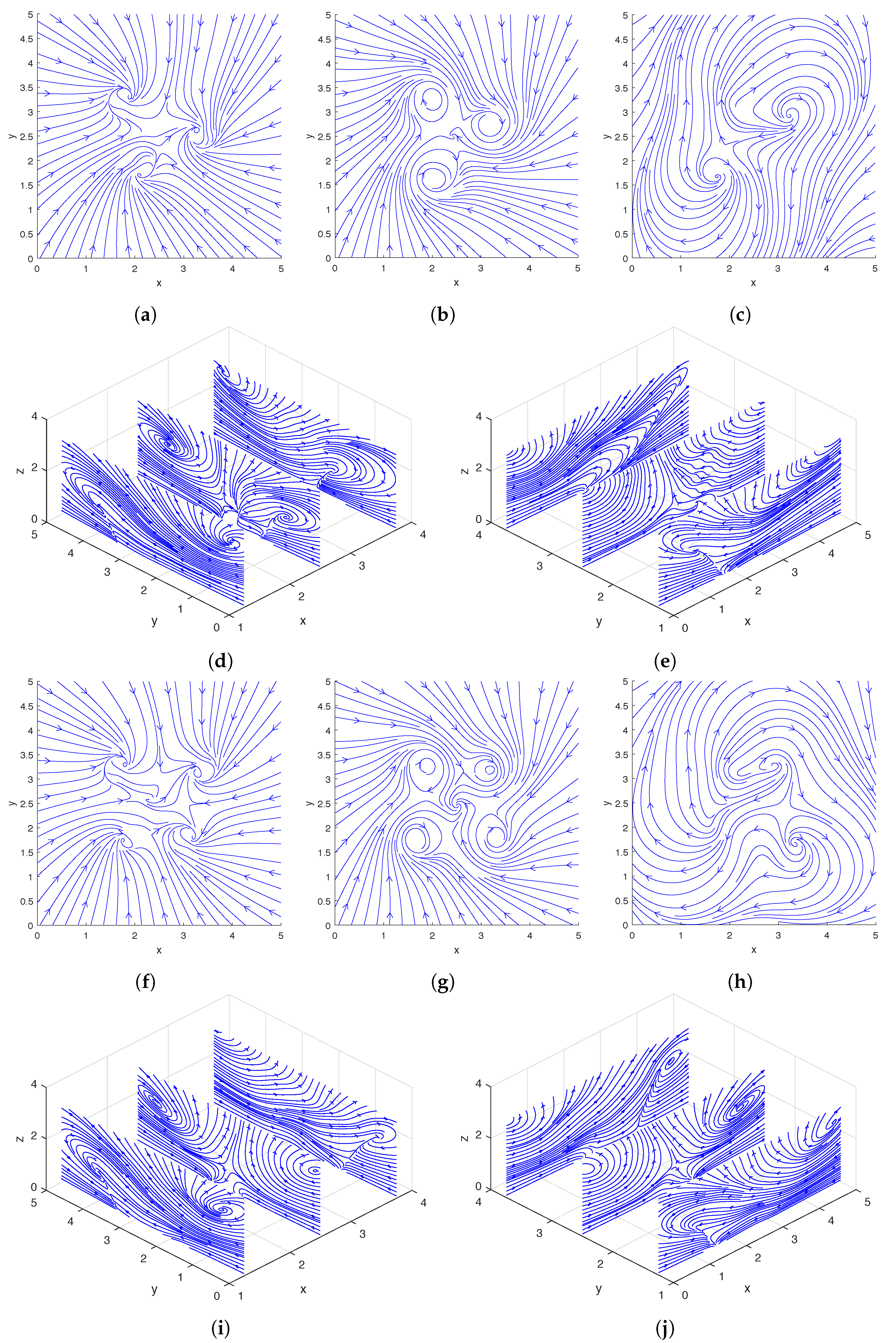
In the top two rows and bottom two rows of Figure 9, we show the streamlines drawn based on the instantaneous fluid velocity around three and four rotating helices, respectively. As can be seen in Figure 9d,e,i,j, the helices move the fluid near their tips upward while rotating.
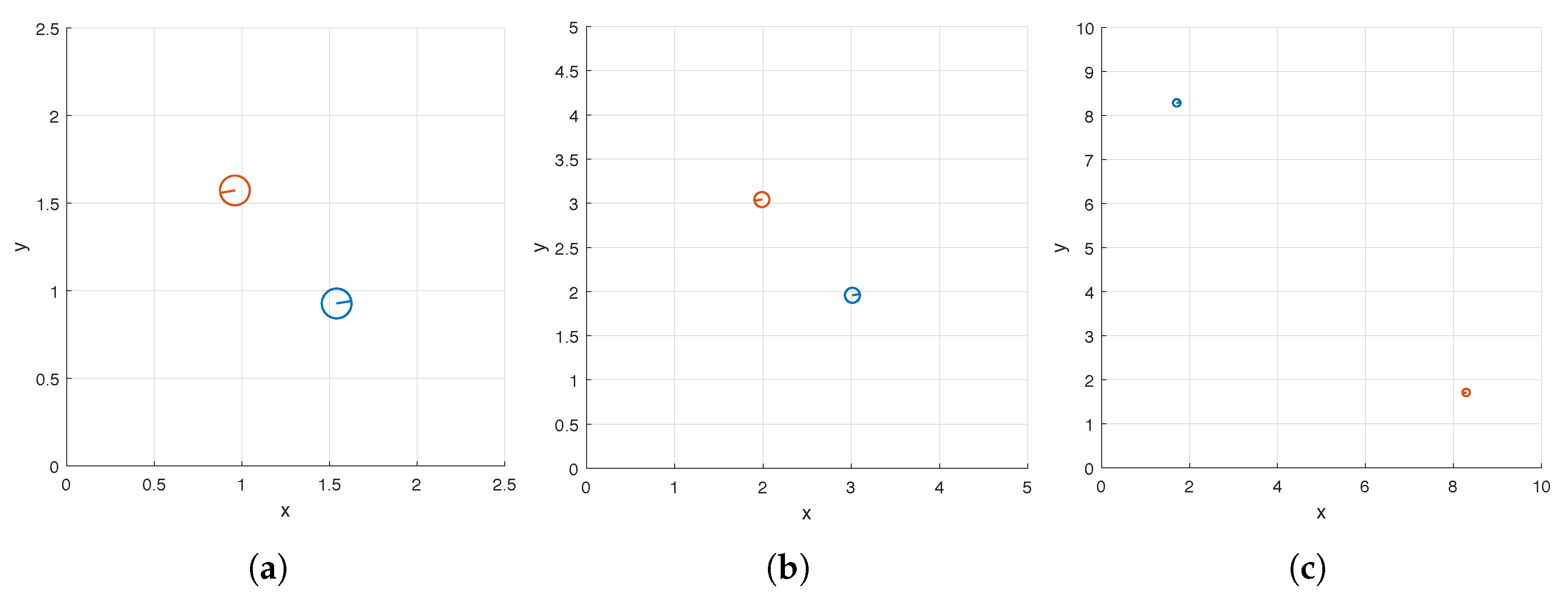
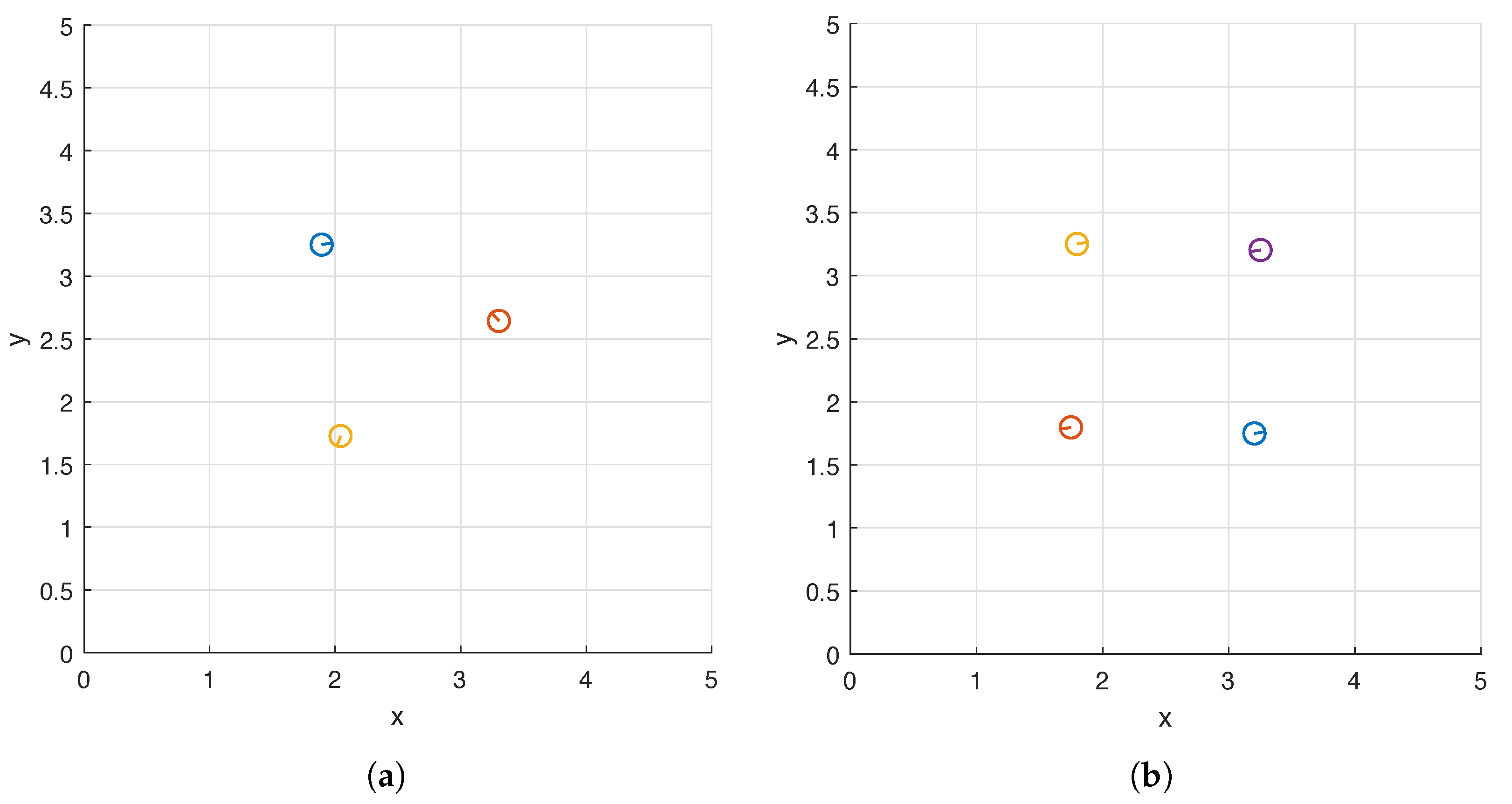
We again consider the square flow meter (7) whose width is and display the top views of the optimal carpets in Figure 10. Interestingly, the helices approximately form an equilateral triangle when there are three of them (Figure 10a) and a square when there are four (Figure 10b) and both shapes are centered at . The differences between the phase shifts of two helices located on adjacent vertices are and in the two cases respectively.
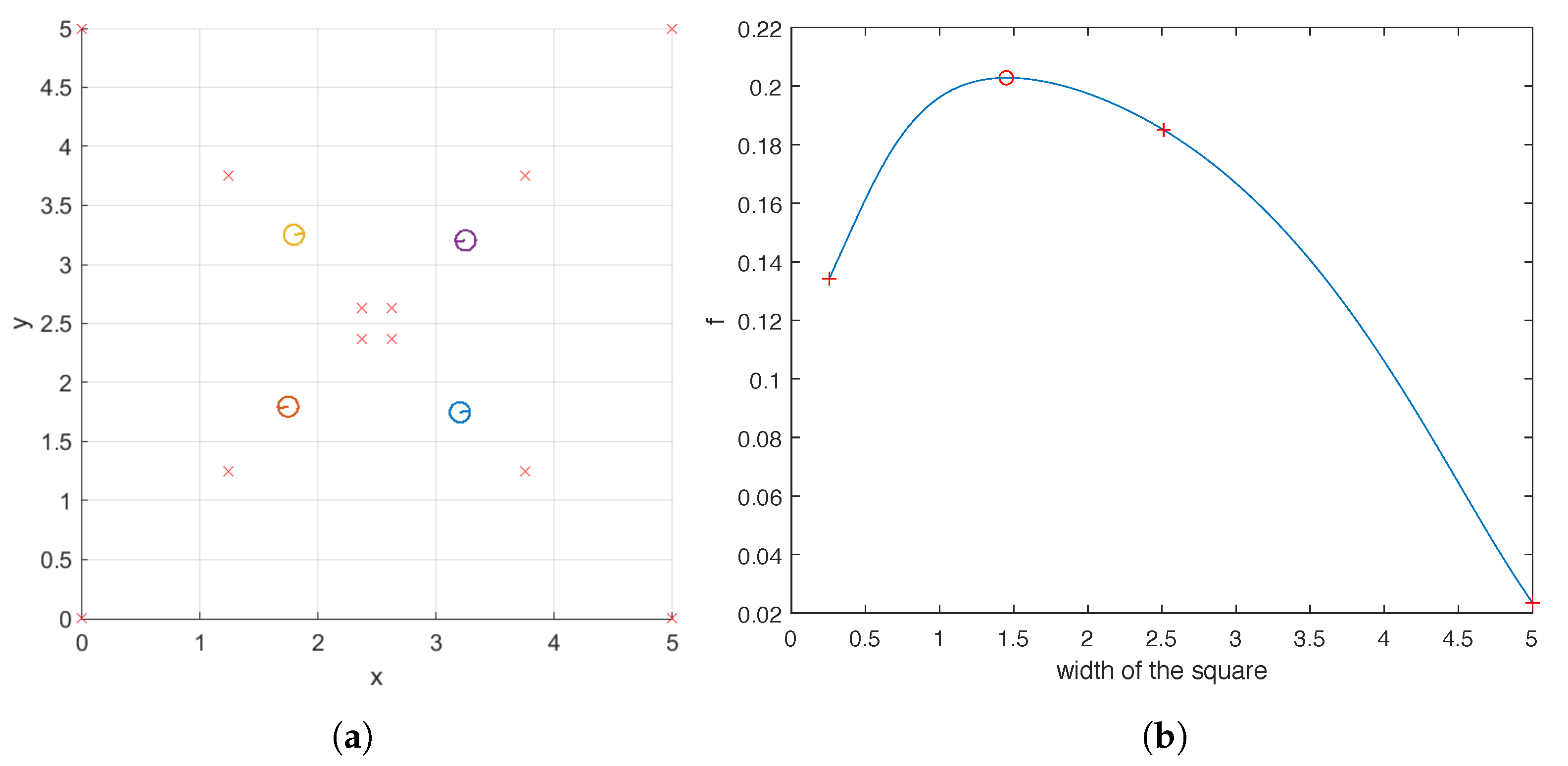
For the case of four helices, we also examine the objective function for a family of carpets which includes the optimal one found by the hybrid method. They share the following properties: the base points of the four helices form a square centered at , each of its four edges is parallel to the x or y axis, and the difference in the phase shifts of two helices located on adjacent vertices is . In Figure 11a, we illustrate three such carpets whose base points are marked by crosses. The optimal carpet found by the hybrid method is also plotted for reference. For this family of carpets, we plot the value of against the width of the square in Figure 11b, which indicates that as the square becomes larger, the ability of the carpet to pump first increases and then decreases, reaching its maximum at the width predicted by the hybrid method. One key observation can be made from Figure 11 that when the four helices are uniformly distributed within the domain , that is, when the width of the square is , the pumping is sub-optimal. Once again, this shows that intuition does not necessarily lead to optimal carpet design.
In Table 8, we report the numbers of iterations, numbers of function evaluations as well as runtimes of the hybrid method. Comparing Table 4, Table 7 and Table 8, we note that the computational cost of the hybrid method increases progressively with the number of helices. This is again due to the growing number of design parameters and cost of evaluating and (see (10) and Table 2).
4. Discussion
We outlined and validated a numerical method for optimizing a fabricated bacterial carpet for fluid pumping through a rectangular flow meter placed just above the helix or helices representing the bacterial flagella. The optimal placement of bacteria in a carpet has many practical applications in biofluidics, as well as the study of food capture or transport of nutrients for or by microorganisms [1,2,8,9,34,35]. To the authors’ knowledge, this is the first study to investigate optimization of carpet design for a flow task or objective. While other methods have previously numerically studied the effects of relative helical positions and phase shifts on pumping [13], this method is the first to study the selection of helical placement and phase shift to maximize fluid pumping.
The optimization problems considered here are challenging for several reasons. Firstly, local maximizers that are not global do exist, and gradient-based methods can converge quickly to these, missing a global maximizer. Secondly, the chosen objective function is not explicitly known, and evaluating it entails computationally expensive fluid simulations. Our approach first employs a GA to perform a global search for an initial solution, then uses this as the starting point for a gradient-based method to perform local searches for the optimal carpet. The GA is applied to a surrogate model for the objective function, which uses coarser temporal and spatial discretization to reduce computational costs. Once an initial solution is found by the GA, the gradient-based method is able to quickly and accurately identify a maximizer in its local vicinity.
The framework developed here is versatile and not limited to optimizing pumping or by the measurement tool employed here (the flow meter). It could also be adapted to consider more design parameters. That is, the carpet could be optimized for mixing or any other fluid task for which an objective function can be determined, or for other helical parameters. For example, since tilt plays an important role in pumping with synthetic flagella for biomedical devices [12,36], we might include tilt in future studies. This would introduce new complications since, for example with multiple helices, solving the optimization problem will be more complicated to avoid flagella physically overlapping.
Our results show that, with the current measurement of pumping, the optimal carpet design depends significantly on the size of the flow meter. Intuitive designs, such as uniform placement, do not always lead to a high-performance carpet. These results highlight the importance of quantitative analysis.
We observed that computing an optimal carpet becomes substantially more expensive as the number of helices increases. At one level, the efficiency of the GA could be improved by using custom methods for crossover and mutation that are more tailored to bacterial carpets. At another level, we want to reduce the computational costs associated with fluid simulation. For example, we might consider implementing regularized Stokeslet segments to reduce the number of points used to model the helices [37]. Additionally, when the number of helices is large, more sophisticated methods must be applied to solve for the forces exerted by the helices on the fluid [38] and calculate the fluid velocities from helical forces [39].
Author Contributions
Conceptualization, M.W.R., A.B., E.S. and L.Z.; methodology, M.W.R.; software, M.W.R.; validation, M.W.R. and W.L.; formal analysis, M.W.R. and W.L.; investigation, M.W.R. and W.L.; resources, M.W.R. and W.L.; data curation, M.W.R.; writing—original draft preparation, M.W.R., A.B., E.S. and L.Z.; writing—review and editing, M.W.R., W.L., A.B., E.S. and L.Z.; visualization, M.W.R., W.L. and L.Z.; funding acquisition, M.W.R. and E.S. All authors have read and agreed to the published version of the manuscript.
Funding
M.W.R. and W.L. were supported, in part, by the National Science Foundation under grant DMS-1818833 (PI: M.W.R.).
Data Availability Statement
The data presented in this study are available on request from the corresponding author.
Acknowledgments
The authors would like to thank the Department of Mathematics and Statistics at James Madison University for supporting a collaborative research meeting in 2019. L Zhao also thanks the support of ACES+ ADVANCE Opportunity Grant from CWRU.
Conflicts of Interest
The authors declare no conflict of interest.
References
- Darnton, N.; Turner, L.; Breuer, K.; Berg, H.C. Moving fluid with bacterial carpets. Biophys. J. 2004, 86, 1863–1870. [Google Scholar] [CrossRef] [Green Version]
- Kim, M.J.; Breuer, K.S. Use of bacterial carpets to enhance mixing in microfluidic Systems. J. Fluids Eng. 2006, 129, 319–324. [Google Scholar] [CrossRef] [Green Version]
- Purcell, E.M. The efficiency of propulsion by a rotating flagellum. Proc. Natl. Acad. Sci. USA 1997, 94, 11307–11311. [Google Scholar] [CrossRef] [PubMed] [Green Version]
- Liu, B.; Breuer, K.S.; Powers, T.R. Helical swimming in Stokes flow using a novel boundary-element method. Phys. Fluids 2013, 25, 061902. [Google Scholar] [CrossRef] [Green Version]
- Liu, B.; Powers, T.R.; Breuer, K.S. Force-free swimming of a model helical flagellum in viscoelastic fluids. Proc. Natl. Acad. Sci. USA 2011, 108, 19516–19520. [Google Scholar] [CrossRef] [Green Version]
- Shields, A.R.; Fiser, B.L.; Evans, B.A.; Falvo, M.R.; Washburn, S.; Superfine, R. Biomimetic cilia arrays generate simultaneous pumping and mixing regimes. Proc. Natl. Acad. Sci. USA 2010, 107, 15670–15675. [Google Scholar] [CrossRef] [Green Version]
- Hanasoge, S.; Hesketh, P.; Alexeev, A. Microfluidic pumping using artificial magnetic cilia. Microsyst. Nanoeng. 2018, 4. [Google Scholar] [CrossRef] [Green Version]
- Stone, H.; Stroock, A.; Ajdari, A. Engineering flows in small devices: Microfluidics toward a lab-on-a-Chip. Annu. Rev. Fluid Mech. 2004, 36, 381–411. [Google Scholar] [CrossRef] [Green Version]
- Hesse, W.R.; Kim, M.J. Visualization of flagellar interactions on bacterial carpets. J. Microsc. 2009, 233, 302–308. [Google Scholar] [CrossRef]
- Kim, H.; Cheang, U.K.; Kim, D.; Ali, J.; Kim, M.J. Hydrodynamics of a self-actuated bacterial carpet using microscale particle image velocimetry. Biomicrofluidics 2015, 9, 024121. [Google Scholar] [CrossRef] [Green Version]
- Lauga, E. Bacterial hydrodynamics. Annu. Rev. Fluid Mech. 2016, 48, 105–130. [Google Scholar] [CrossRef] [Green Version]
- Buchmann, A.; Fauci, L.; Leiderman, K.; Strawbridge, E.; Zhao, L. Flow induced by bacterial carpets and transport of microscale loads. In Applications of Dynamical Systems in Biology and Medicine; Jackson, T., Radunskaya, A., Eds.; Springer: New York, NY, USA, 2015; Volume 158, The IMA Volumes in Mathematics and its Applications; pp. 35–53. [Google Scholar] [CrossRef]
- Buchmann, A.; Fauci, L.J.; Leiderman, K.; Strawbridge, E.; Zhao, L. Mixing and pumping by pairs of helices in a viscous fluid. Phys. Rev. E 2018, 97, 023101. [Google Scholar] [CrossRef] [Green Version]
- Mathijssen, A.J.T.M.; Guzmán-Lastra, F.; Kaiser, A.; Löwen, H. Nutrient transport driven by microbial active carpets. Phys. Rev. Lett. 2018, 121, 248101. [Google Scholar] [CrossRef] [Green Version]
- Ding, Y.; Nawroth, J.C.; McFall-Ngai, M.J.; Kanso, E. Mixing and transport by ciliary carpets: A numerical study. J. Fluid Mech. 2014, 743, 124–140. [Google Scholar] [CrossRef] [Green Version]
- Goldberg, D.E. Genetic Algorithms in Search, Optimization and Machine Learning, 1st ed.; Addison-Wesley Longman Publishing Co., Inc.: Boston, MA, USA, 1989. [Google Scholar]
- Mitchell, M. An Introduction to Genetic Algorithms; MIT Press: Cambridge, MA, USA, 1998. [Google Scholar]
- Whitley, D. A genetic algorithm tutorial. Stat. Comput. 1994, 4, 65–85. [Google Scholar] [CrossRef]
- Curry, H.B. The method of steepest descent for non-linear minimization problems. Q. Appl. Math. 1944, 2, 258–261. [Google Scholar] [CrossRef] [Green Version]
- Lemaréchal, C. Cauchy and the gradient method. Doc. Math. 2012, Extra Volume ISMP, 251–254. [Google Scholar]
- Broyden, C.G. The convergence of a class of double-rank minimization algorithms: 1. General considerations. IMA J. Appl. Math. 1970, 6, 76–90. [Google Scholar] [CrossRef]
- Broyden, C.G. The convergence of a class of double-rank minimization algorithms: 2. The new algorithm. IMA J. Appl. Math. 1970, 6, 222–231. [Google Scholar] [CrossRef] [Green Version]
- Fletcher, R. A new approach to variable metric algorithms. Comput. J. 1970, 13, 317–322. [Google Scholar] [CrossRef] [Green Version]
- Goldfarb, D. A family of variable-metric methods derived by variational means. Math. Comput. 1970, 24, 23–26. [Google Scholar] [CrossRef]
- Shanno, D.F. Conditioning of quasi-Newton methods for function minimization. Math. Comput. 1970, 24, 647–656. [Google Scholar] [CrossRef]
- Cortez, R. The method of regularized Stokeslets. SIAM J. Sci. Comput. 2001, 23, 1204–1225. [Google Scholar] [CrossRef]
- Cortez, R.; Fauci, L.; Medovikov, A. The method of regularized Stokeslets in three dimensions: Analysis, validation, and application to helical swimming. Phys. Fluids 2005, 17, 031504. [Google Scholar] [CrossRef]
- Ainley, J.; Durkin, S.; Embid, R.; Boindala, P.; Cortez, R. The method of images for regularized Stokeslets. J. Comput. Phys. 2008, 227, 4600–4616. [Google Scholar] [CrossRef]
- Leiderman, K.; Bouzarth, E.L.; Cortez, R.; Layton, A.T. A regularization method for the numerical solution of periodic Stokes flow. J. Comput. Phys. 2013, 236, 187–202. [Google Scholar] [CrossRef]
- Nguyen, H.N.; Leiderman, K. Computation of the singular and regularized image systems for doubly-periodic Stokes flow in the presence of a wall. J. Comput. Phys. 2015, 297, 442–461. [Google Scholar] [CrossRef]
- Zhong, S.; Moored, K.; Pinedo, V.; Garcia-Gonzalez, J.; Smits, A. The flow field and axial thrust generated by a rotating rigid helix at low Reynolds numbers. Exp. Therm. Fluid Sci. 2013, 46, 1–7. [Google Scholar] [CrossRef]
- Meng, F.; Bennett, R.R.; Uchida, N.; Golestanian, R. Conditions for metachronal coordination in arrays of model cilia. Proc. Natl. Acad. Sci. USA 2021, 118. [Google Scholar] [CrossRef] [PubMed]
- Chakrabarti, B.; Fürthauer, S.; Shelley, M.J. A multiscale biophysical model gives quantized metachronal waves in a lattice of cilia. arXiv 2021, arXiv:cond-mat.soft/2108.01693. [Google Scholar]
- Beebe, D.J.; Mensing, G.A.; Walker, G.M. Physics and applications of microfluidics in biology. Annu. Rev. Biomed. Eng. 2002, 4, 261–286. [Google Scholar] [CrossRef] [PubMed]
- Rusconi, R.; Garren, M.; Stocker, R. Microfluidics expanding the frontiers of microbial ecology. Annu. Rev. Biophys. 2014, 43, 65–91. [Google Scholar] [CrossRef] [PubMed] [Green Version]
- Zhao, L. Fluid-Structure Interaction in Viscous Dominated Flows. Ph.D. Thesis, The University of North Carolina at Chapel Hill, Chapel Hill, NC, USA, 2010. [Google Scholar]
- Cortez, R. Regularized Stokeslet segments. J. Comput. Phys. 2018, 375, 783–796. [Google Scholar] [CrossRef] [Green Version]
- Rostami, M.W.; Olson, S.D. Fast algorithms for large dense matrices with applications to biofluids. J. Comput. Phys. 2019, 394, 364–384. [Google Scholar] [CrossRef]
- Rostami, M.W.; Olson, S.D. Kernel-independent fast multipole method within the framework of regularized Stokeslets. J. Fluids Struct. 2016, 67, 60–84. [Google Scholar] [CrossRef]
Figure 1.
A sketch of a carpet consisting of two helices and a square flow meter (7) above it. The top view of the helices is also shown. The bases of the helices are attached to an infinite, planar, and solid wall located at .
Figure 1.
A sketch of a carpet consisting of two helices and a square flow meter (7) above it. The top view of the helices is also shown. The bases of the helices are attached to an infinite, planar, and solid wall located at .

Figure 2.
Streamlines of the flow around a single rotating helix at the midpoint of a cycle. The location and phase shift of the helix are shown in Figure 3c. Top row: Streamlines plotted using only the x- and y-direction fluid velocities on the slice planes located at (a), (b), and (c). Bottom row: Streamlines plotted using only the y- and z-direction fluid velocities on the slice planes located at (d); streamlines plotted using only the x- and z-direction fluid velocities on the slice planes located at (e).

Figure 3.
The top views of the optimal carpets found by the hybrid method (a,c,e) and the surface and contour plots of (b,d,f) in the case of a single helix. The three rows correspond to three sizes of the flow meter (7): (a,b), 5 (c,d), and 10 (e,f).
Figure 3.
The top views of the optimal carpets found by the hybrid method (a,c,e) and the surface and contour plots of (b,d,f) in the case of a single helix. The three rows correspond to three sizes of the flow meter (7): (a,b), 5 (c,d), and 10 (e,f).

Figure 4.
Contour plots of the z-direction velocity on the flow meter (7) with at the midpoint of a cycle in the case of a single rotating helix. The phase shift of the helix is 0. (a): The location of the helix is shown in Figure 3e. (b): The helix is based at , the center of the domain.

Figure 5.
The estimate found by Step 1 of the hybrid method and the runtime of this step as the seed of the random number generators varies for the case of a single helix. The flow meter is (7) with . Step 1 is repeated sixty-four times and a different seed is used each time. (a): Clustering of the sixty-four ’s around the four maximizers of . (b): Histogram of the sixty-four runtimes.

Figure 6.
Streamlines drawn from the flow around a pair of rotating helices at the midpoint of a cycle. The locations and phase shifts of the helices are shown in Figure 7b. Top row: Streamlines plotted using only the x- and y-direction fluid velocities on the slice planes located at (a), (b), and (c). Bottom row: Streamlines plotted using only the y- and z-direction fluid velocities on the slice planes located at (d); streamlines plotted using only the x- and z-direction fluid velocities on the slice planes located at (e).

Figure 7.
Top views of the optimal carpets consisting of a pair of helices found by the hybrid method. The three panels correspond to three sizes of the flow meter (7): (a), 5 (b), and 10 (c).
Figure 7.
Top views of the optimal carpets consisting of a pair of helices found by the hybrid method. The three panels correspond to three sizes of the flow meter (7): (a), 5 (b), and 10 (c).

Figure 8.
The graph of as the location of one helix varies along a straight line while the location of the other helix and the phase shifts of both helices remain fixed. The two rows correspond to two sizes of the flow meter (7): (a,b) and 10 (c,d). (a,c): The top view of the optimal carpet with the path of the moving helix marked by a dashed line. (b,d): The value of as the distance between the base points of the helices increases. In (a–d), the crosses correspond to a few sample locations along the dashed line.

Figure 9.
Streamlines drawn from the flow around three (a–e) and four (f–j) rotating helices at the midpoint of a cycle. The locations and phase shifts of the helices in the two cases are shown in Figure 10a,b respectively. (a–c) and (f–h): Streamlines plotted using only the x- and y-direction fluid velocities on the slice planes located at (a,f), (b,g), and (c,h). (d,i): Streamlines plotted using only the y- and z-direction fluid velocities on the slice planes located at . (e,j): Streamlines plotted using only the x- and z-direction fluid velocities on the slice planes located at .

Figure 10.
The top views of the optimal carpets consisting of three (a) and four (b) helices found by the hybrid method. The flow meter is (7) with .
Figure 10.
The top views of the optimal carpets consisting of three (a) and four (b) helices found by the hybrid method. The flow meter is (7) with .

Figure 11.
The base points of helices belonging to a few square carpets (a) and the value of as the width of the square increases (b). The three crosses in (b) correspond to the three carpets marked by crosses in (a). The difference in the phase shifts of two helices located on adjacent vertices is . The flow meter is (7) with .


Table 1.
Default parameter values given in non-dimensional units.
| Parameter | Description | Value |
|---|---|---|
| blob size | 0.01 (for f) or 0.1 (for s) | |
| viscosity | 1 | |
| L | axial length of helix | 2.2 |
| helical radius | 0.085 | |
| tapering parameter | 1000 | |
| helical pitch | ||
| angular speed | ||
| n | points per helix | 158 (for f) or 16 (for s) |
| T | time to perform one rotation | |
| number of time steps per rotation | 1000 (for f) or 100 (for s) | |
| flow meter location | 2.5 |
Table 2.
The runtimes of evaluating and when the carpet consists of one, two, or four helices and the width of the flow meter (7) is , 5, or 10.
Table 2.
The runtimes of evaluating and when the carpet consists of one, two, or four helices and the width of the flow meter (7) is , 5, or 10.
| W | One Helix | Two Helices | Four Helices | |||
|---|---|---|---|---|---|---|
| 165 | 449 | 763 | ||||
| 5 | 244 | 823 | 1365 | |||
| 10 | 489 | 1416 | 2494 | |||
Table 3.
The maximizers found by the hybrid method for the case of a single helix and three sizes of the flow meter (7): , 5, and 10.
Table 3.
The maximizers found by the hybrid method for the case of a single helix and three sizes of the flow meter (7): , 5, and 10.
| W | Step 1: GA Applied to s | Step 2: BFGS Applied to f |
|---|---|---|
| 5 | ||
| 10 |
Table 4.
The runtimes, iteration counts, and numbers of function evaluations entailed by the hybrid method for the case of a single helix and three sizes of the flow meter (7): , 5, and 10. (Forty-eight computer cores are used).
Table 4.
The runtimes, iteration counts, and numbers of function evaluations entailed by the hybrid method for the case of a single helix and three sizes of the flow meter (7): , 5, and 10. (Forty-eight computer cores are used).
| W | Step 1: GA Applied to s | Step 2: BFGS Applied to f | Total | ||||
|---|---|---|---|---|---|---|---|
| # of Iter. | # of s Eval. | Runtime | # of Iter. | # of f Eval. | Runtime | Runtime | |
| 66 | 3350 | 877 | 2 | 12 | 207 | 1084 | |
| 5 | 53 | 2700 | 1170 | 3 | 18 | 386 | 1556 |
| 10 | 64 | 3250 | 1717 | 2 | 15 | 461 | 2178 |
Table 5.
The maximizers found by the GA and the runtimes, iteration counts, and numbers of function evaluations entailed by the GA for the case of a single helix and three sizes of the flow meter (7): , 5, and 10. (Forty-eight computer cores are used).
Table 5.
The maximizers found by the GA and the runtimes, iteration counts, and numbers of function evaluations entailed by the GA for the case of a single helix and three sizes of the flow meter (7): , 5, and 10. (Forty-eight computer cores are used).
| W | # of Iter. | # of f Eval. | Runtime | |
|---|---|---|---|---|
| 67 | 3400 | 19,639 | ||
| 5 | 55 | 2800 | 24,784 | |
| 10 | 64 | 3250 | 38,741 |
Table 6.
The maximizers found by the hybrid method for the case of a pair of helices and three sizes of the flow meter (7): , 5, and 10.
Table 6.
The maximizers found by the hybrid method for the case of a pair of helices and three sizes of the flow meter (7): , 5, and 10.
| W | Step 1: GA Applied to s | Step 2: BFGS Applied to f | ||||
|---|---|---|---|---|---|---|
| 5 | ||||||
| 10 | ||||||
Table 7.
The runtimes, iteration counts, and numbers of function evaluations entailed by the hybrid method for the case of a pair of helices and three sizes of the flow meter (7): , 5, and 10. (Forty-eight computer cores are used).
Table 7.
The runtimes, iteration counts, and numbers of function evaluations entailed by the hybrid method for the case of a pair of helices and three sizes of the flow meter (7): , 5, and 10. (Forty-eight computer cores are used).
| W | Step 1: GA Applied to s | Step 2: BFGS Applied to f | Total | ||||
|---|---|---|---|---|---|---|---|
| # of Iter. | # of s Eval. | Runtime | # of Iter. | # of f Eval. | Runtime | Runtime | |
| 105 | 5300 | 2174 | 19 | 132 | 2595 | 4769 | |
| 5 | 68 | 3450 | 2021 | 17 | 114 | 4273 | 6294 |
| 10 | 120 | 6050 | 6229 | 4 | 42 | 2565 | 8794 |
Table 8.
The runtimes, iteration counts, and numbers of function evaluations entailed by the hybrid method for the cases of three and four helices. The flow meter is (7) with . (Forty-eight computer cores are used).
Table 8.
The runtimes, iteration counts, and numbers of function evaluations entailed by the hybrid method for the cases of three and four helices. The flow meter is (7) with . (Forty-eight computer cores are used).
| # of | Step 1: GA Applied to s | Step 2: BFGS Applied to f | Total | ||||
|---|---|---|---|---|---|---|---|
| Helices | # of Iter. | # of s Eval. | Runtime | # of Iter. | # of f Eval. | Runtime | Runtime |
| three | 78 | 15,800 | 12,479 | 6 | 136 | 8615 | 21,094 |
| four | 159 | 32,000 | 30,178 | 38 | 450 | 45,729 | 75,907 |
Publisher’s Note: MDPI stays neutral with regard to jurisdictional claims in published maps and institutional affiliations. |
© 2022 by the authors. Licensee MDPI, Basel, Switzerland. This article is an open access article distributed under the terms and conditions of the Creative Commons Attribution (CC BY) license (https://creativecommons.org/licenses/by/4.0/).
Share and Cite
MDPI and ACS Style
Rostami, M.W.; Liu, W.; Buchmann, A.; Strawbridge, E.; Zhao, L. Optimal Design of Bacterial Carpets for Fluid Pumping. Fluids 2022, 7, 25. https://doi.org/10.3390/fluids7010025
AMA Style
Rostami MW, Liu W, Buchmann A, Strawbridge E, Zhao L. Optimal Design of Bacterial Carpets for Fluid Pumping. Fluids. 2022; 7(1):25. https://doi.org/10.3390/fluids7010025
Chicago/Turabian StyleRostami, Minghao W., Weifan Liu, Amy Buchmann, Eva Strawbridge, and Longhua Zhao. 2022. "Optimal Design of Bacterial Carpets for Fluid Pumping" Fluids 7, no. 1: 25. https://doi.org/10.3390/fluids7010025