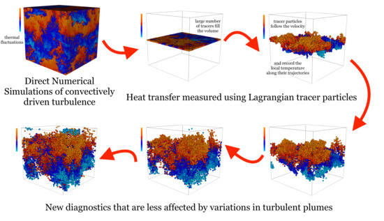
Lagrangian Statistics of Heat Transfer in Homogeneous Turbulence Driven by Boussinesq Convection


1
Department of Physics and Astronomy, Georgia State University, Atlanta, GA 30303, USA
2
James Watt School of Engineering, University of Glasgow, Glasgow G12 8QQ, UK
3
Center for Astronomy and Astrophysics, ER 3-2, TU Berlin, Hardenbergstr. 36, 10623 Berlin, Germany
*
Author to whom correspondence should be addressed.
Fluids 2020, 5(3), 127; https://doi.org/10.3390/fluids5030127
Submission received: 29 June 2020
/
Revised: 26 July 2020
/
Accepted: 29 July 2020
/
Published: 3 August 2020
(This article belongs to the Special Issue Lagrangian Transport in Geophysical Fluid Flows)
Abstract
:The movement of heat in a convecting system is typically described by the nondimensional Nusselt number, which involves an average over both space and time. In direct numerical simulations of turbulent flows, there is considerable variation in the contributions to the Nusselt number, both because of local spatial variations due to plumes and because of intermittency in time. We develop a statistical approach to more completely describe the structure of heat transfer, using an exit-distance extracted from Lagrangian tracer particles, which we call the Lagrangian heat structure. In a comparison between simulations of homogeneous turbulence driven by Boussinesq convection, the Lagrangian heat structure reveals significant non-Gaussian character, as well as a clear trend with Prandtl number and Rayleigh number. This has encouraging implications for simulations performed with the goal of understanding turbulent convection in natural settings such as Earth’s atmosphere and oceans, as well as planetary and stellar dynamos.
1. Introduction
Convection occurs in many natural settings, including the oceans, the atmosphere, and the interior of the Earth and the stars. These convective flows are not typically constrained by solid boundaries, and therefore have some characteristics that differ from experimental set-ups like Rayleigh-Bénard convection. Convection-driven flow in natural systems is often turbulent, but may be unaffected by boundary layers, large-scale circulations, or regular convection rolls. These large-scale flow features may be absent, or they may be so large that they do not influence the local characteristics of the turbulence. Thus convective turbulence in the interior of an atmospheric layer or the interior of a stellar convection zone appears homogeneous on scales smaller than the pressure scale-height. These are the length scales accessible to study with direct numerical simulations.
Early studies of convection in natural settings focused heavily on the development of Lagrangian statistics to describe diffusion and dispersion, e.g., Gifford [1], Roberts [2], Sutton [3], Frenkiel and Katz [4], Kellogg [5]. Lagrangian tracer particles continue to be widely regarded as an ideal way to describe turbulent diffusion and transport (see for example [6,7]). Recent work using Lagrangian statistics to examine fundamental properties of turbulent convection is delivering a wealth of new insight into these processes [8,9,10,11,12,13]. Exit-time and exit-distance statistics, sometimes also called first-passage times, can be produced with Lagrangian particles, and have been shown to provide useful information that minimizes the effect of intermittency. Popular examples of exit-time and exit-distance statistics are the doubling-time [14], finite-size Lyapunov exponents (FSLE) [15,16,17,18], finite-time Lyapunov exponents (FTLE), and inverse structure functions [19,20].
The heat transfer is one of the most fundamental aspects of convection. Measuring the evolving temperature, and how it correlates with velocity, is a problem of active interest for oceanographers and atmospheric scientists (e.g., as discussed by [21]). Experimental investigations of convection [8,13,22] have recently engineered smart particles that can sense and record the temperature that they experience in a turbulent flow. This experimental development also increases our need to define clearer theoretical measures to understand heat transfer in turbulent convection.
Heat transfer has typically been approached using a dimensionless heat flux averaged over the simulation time and volume, called the Nusselt number (). However, in many cases the Nusselt number describes the heat transfer in a limited way. This is particularly true in simulations of homogeneous turbulent convection, where the most relevant dynamical length scale is not necessarily associated with the imposed temperature gradient, and the dynamical length scale of the flow may actively change and evolve. A wide variation of the Nusselt number in both space and time results. Intermittency can be observed for different diagnostics in a wide range of turbulent flows [23], including stratified turbulence relevant to geophysical fluids (e.g., [24].) For comparing different realizations of homogeneous turbulent convection, a more detailed description of the heat flux is needed. In this work we therefore discuss the development of a new higher order statistic related to the heat transfer.
We build this new statistic as a Lagrangian exit-distance statistic to characterize how heat is transported over distances in a turbulent flow. The use of an exit-distance statistic has the advantage, documented in Lagrangian descriptions of turbulence [18], that it permits us to compare fluid particles that have transported the same amount in temperature, rather than particles that have diffused for the same length of time. This removes contamination due to crossover from other temperature scales, a quality that has helped to clarify intermittent behavior in hydrodynamic turbulence (e.g., as discussed in [25]). Examination of this statistic provides higher-order information about the heat transfer from a different perspective, supplementing a straightforward global average like the Nusselt number.
Heat transfer and heat flux are highly dependent on a fluid’s Prandtl number, the ratio of viscosity to thermal diffusivity (e.g., [26,27,28]). The fundamental idea is that low flows can support small-scale velocity fluctuations while the corresponding small-scale temperature fluctuations are smoothed out by diffusion; the opposite situation occurs at large . In the oceans, viscosity dominates and the Prandtl number ranges between approximately 7 (warm sea water) to 13 (sea water near freezing). Atmospheric convection occurs in the air, where the Prandtl number can range between and with a typical value of 0.72 for air. In the solar convection zone thermal diffusivity dominates, and Prandtl numbers on the order of to are estimated. Current direct numerical studies of convection typically are able to describe a range of Prandtl numbers between (e.g., [29,30]), while dynamo studies often focus on . A more detailed theoretical understanding of how the dynamics of thermal fluctuations change when different Prandtl numbers are considered is key to effectively modeling convection in these different settings. Using our new Lagrangian exit-distance statistic, the Lagrangian heat structure, we compare simulations of turbulent convection over the range of Prandtl numbers . This comparison illustrates the utility of the Lagrangian heat structure to expose differences in the transport of heat.
This work is structured as follows. In Section 2 we describe the physical and numerical models used to produce simulations of homogeneous turbulent Boussinesq convection at different Prandtl numbers. In Section 3 we discuss the Nusselt number and its variation during our simulations. In Section 4 we derive a Lagrangian exit-distance statistic to provide more detail about the heat transfer than can be extracted from the Nusselt number. We present the results of this new diagnostic for our simulations. In Section 5 we discuss the implications of these results.
2. Simulations
We perform direct numerical simulations of homogeneous turbulence driven by Boussinesq convection. In each simulation, the dynamical equations are solved using a pseudospectral method in a cubic simulation volume with a side of length . The nondimensional equations for Navier-Stokes turbulence driven by Boussinesq convection are
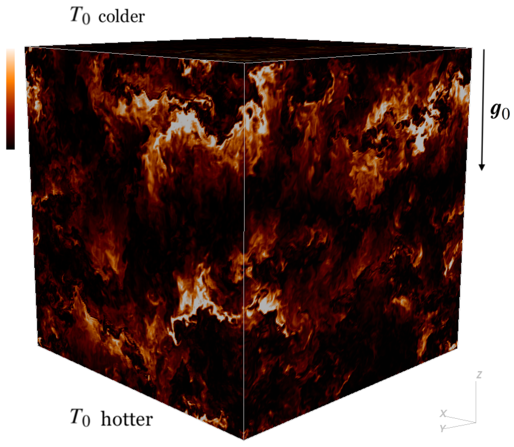
These equations include the solenoidal velocity field v, the vorticity , and the thermal fluctuation about the mean temperature . In our fluid model, the total temperature is expressed as the sum of mean and fluctuating quantities: . The turbulent flow is driven solely by the fixed, unitary, mean temperature gradient in the vertical direction, opposing the direction of gravity; the gradient of the mean temperature can be expressed fully by the z-component . In Equation (1), is a unit vector in the direction of gravity; the term that includes is commonly known as the buoyancy force. The simulation volume and physical set-up are indicated alongside a visualization of thermal energy in Figure 1. Two dimensionless parameters appear in the equations: and . They derive from the kinematic viscosity and the thermal diffusivity , and are defined so that the Prandtl number . The thermal diffusivity relates to the nondimensional quantity by . A low-storage third-order Runge-Kutta method [31] is used for the time-integration of Equations (1)–(3).
Boundary conditions strongly influence the structure and dynamics of a flow. For convection simulations the choice of fully periodic boundary conditions (sometimes called homogeneous Rayleigh-Bénard boundary conditions) allows a macroscopic elevator instability to form [32], which manifests as an exponentially growing mean velocity component along the direction of gravity. The elevator instability rapidly destroys the turbulent flow field, making it impossible to collect long-time steady-state statistical data. To avoid this, the simulation volume considered in this work is confined by quasi-periodic boundary conditions (as in [33,34,35]). Quasi-periodic boundary conditions explicitly suppress the mean flow parallel to gravity, which is removed at each time step. Our simulations are pseudospectral, and therefore a vertical mean flow is straightforwardly isolated in Fourier space. These boundary conditions are also periodic, like the homogeneous Rayleigh-Bénard boundary conditions. Quasi-periodic boundary conditions combine the conceptual simplicity of statistical homogeneity with a physically natural convective driving of the turbulent flow. With these boundary conditions, a large-scale structuring of the turbulent flow, such as the convection-cell pattern caused by Rayleigh-Bénard boundary conditions does not occur. Unlike Rayleigh-Bénard convection, our simulations therefore produce homogeneous anisotropic convection.
A summary of the fundamental parameters describing each simulation is given in Table 1. In this table, we define the Reynolds number to be , where is the kinetic energy, and the brackets indicate a time-average. For statistically homogeneous turbulent convection the characteristic length scale is the instantaneous temperature gradient length scale where is the root-mean-square of thermal fluctuations [36]. We measure length in units of the Kolmogorov microscale and time in units of the Kolmogorov time-scale , where is the dissipation of kinetic energy; the Kolmogorov scales are the smallest length and time scales that characterize turbulent flows. The Kolmogorov microscale multiplied by , the highest wavenumber in the simulation, is often used to test whether a simulation is adequately resolved on small spatial scales. In this work all of the simulations fulfill the standard criterion used for hydrodynamic turbulence due to Pope [37] for adequate spatial resolution of the velocity field: (). The grid size used and are given in Table 1.
Because this work treats convection at different Prandtl numbers, an independent requirement is necessary to be sure that the field of thermal fluctuations is also adequately resolved. This question has been closely examined for Rayleigh-Beńard convection (e.g., [38,39]), and the Nusselt number has been found to be particularly sensitive to the resolution. In contrast to Rayleigh-Beńard convection, for homogeneous convection we expect that the buoyancy force will be significant, the flow is potentially strongly anisotropic, and strong velocity and temperature gradients can occur with equal probability throughout the flow. For this reason, a resolution criterion for the thermal fluctuations equivalent to that used for the velocity field is desirable in our simulations. By dimensional argument, the equivalent to Pope’s resolution criterion [37] can be straightforwardly extended to the field of thermal fluctuations. The dimension of kinematic viscosity is and the dimension of the kinetic energy dissipation rate is . The only combination of these dimensions that has the dimension of time is the Kolmogorov time-scale . The thermal diffusivity also has units of , and the thermal energy dissipation rate has the same units as the kinetic energy dissipation rate. Thus we define the thermal microscale . We consider the field of thermal energy to be adequately resolved in space if the thermal microscale fulfills the requirement . Each of our simulations also fulfills this criterion. The satisfactory nature of this criterion is clear from a comparison of the average spectra of kinetic and thermal energy for simulations HC1, HC2, HC3, and HC4 (see Figure 2). For simulation HC2 () the kinetic energy and thermal energy experience a similar level of damping. For simulation HC1 () it is clear that the thermal energy spectrum experiences more damping than the kinetic energy spectrum; the reverse is true for simulation HC3 (). For simulation HC4 (), the spectra are similar to HC2, but exhibit a wider inertial range.
2.1. Lagrangian Tracer Particles
Each simulation is launched with random Eulerian fields of unitary magnitude. After a statistically stationary steady state is attained by the convective driving, i.e., when the global kinetic energy has established a well-defined average value in time, the simulation is judged to have produced a physically realistic initial state to begin the calculation of Lagrangian statistics. This period of relaxation lasts more than in each simulation. The positions of Lagrangian tracer particles are then initialized in a homogeneous random distribution. The total number of particles is given in Table 1. This is a standard density of tracer particles for such simulations, and the Lagrangian statistics produced have been tested and found to be well-resolved in space. The Eulerian time step for each simulation is much less than the limit of the CFL number, and chosen so that ; the same time step is used when integrating the trajectories of tracer particles. Lagrangian data is recorded every four Eulerian time steps for post-processing, so that . At each time step the particle velocities, thermal fluctuations, and gradients of these quantities are interpolated from the instantaneous Eulerian velocity field using a tricubic (see for example [40]) polynomial interpolation scheme. Particle positions are calculated by numerical integration of the equation of motion using a third order Runge-Kutta method. Each simulation is run for at least , and the total simulation time is given in Table 1. Our Lagrangian statistics are validated by examining Lagrangian single-particle diffusion, the average square distance a given particle has moved from its initial position. The Lagrangian single-particle diffusion in directions perpendicular and parallel to gravity is shown in Figure 3. In the figure, triangular brackets indicate an average over all Lagrangian particles in the simulation. The diffusion curves perpendicular to gravity exhibit the ballistic scaling with for early times and the diffusive scaling with t for long times. The diffusion curves parallel to gravity are slightly superdiffusive for long times due to the anisotropy introduced by the convective driving.
For the purpose of further validation of our Lagrangian statistics, we examine the Lagrangian autocorrelation functions shown in Figure 4. These have the typical shape known from hydrodynamic turbulence (e.g., [6]); they are initially one, and decay smoothly to zero at long times without ever becoming negative. Velocity autocorrelation functions have been examined more recently to determine the anisotropy of magnetohydrodynamic (e.g., [41]), and rotating stratified systems (e.g., [42]). In Figure 4, the decay of the autocorrelation function of takes place over a slightly longer time than the autocorrelation of velocity in the direction parallel to gravity. The velocities in the plane perpendicular to gravity have a much shorter correlation time, due to the anisotropy that convection introduces to the system. For simulation HC1 () this decay time is more than twice as long as simulation HC3 (). A longer decay time is to be expected for simulation HC1 than for HC3, since the lower Prandtl number is achieved by using a lower viscosity.
2.2. Rayleigh Number
The Rayleigh number is a dimensionless measure of the convective driving: the product of the Prandtl number with the Grashof number, the ratio of the buoyancy to viscous force acting on a fluid. In comparisons of convecting systems, the Rayleigh number is typically held constant when the Prandtl number is varied so that results are compared from systems with identical convective driving. The Rayleigh number is typically defined by , where is the temperature difference across the fluid layer of height L. Because our system is periodic, the typical temperature difference across any height of fluid is defined only by the mean temperature gradient that we impose. This contrasts with the boundary conditions that are typically used in Rayleigh-Bénard convection, and has consequences for several nondimensional parameters that characterize a convecting system. Our mean temperature gradient is unitary, and therefore for . Adopting for the length scale of the fluid layer is a sensible choice in our nondimensional, periodic system; this length scale should be fixed to allow for the Rayleigh number to be well-defined. The quantities g and are also one in our nondimensional units. We therefore calculate the Rayleigh number for our homogeneous simulations in nondimensional units using . This Rayleigh number is held fixed at for the three simulations HC1, HC2, and HC3 described in Table 1. This is the highest Rayleigh number achievable using a grid size of while also maintaining our criterion for adequate spatial resolution of the turbulent velocity and thermal fluctuations described above for the three simulations at different Prandtl numbers. The three simulations HC1, HC2, and HC3 provide a comparison of different Prandtl number flows at fixed Rayleigh number; simulations HC1 and HC4 provide a useful comparison of different Prandtl number flows at fixed Grashof number (e.g., [29]). Simulation HC4 uses a Rayleigh number that is ten times higher than simulation HC2, to allow for a comparison between results at different Rayleigh numbers for fixed Prandtl number.
3. Results: Nusselt Number
This definition is constructed using the total heat flux , where T is the total temperature in dimensionless units. The triangular brackets indicate an averaging over the simulation volume and the simulation time t. The change in temperature and length scale L are positive quantities, identical to the quantities used in the definition of the Rayleigh number. In our system the mean temperature gradient is constant and linear, so that . Using these definitions, the nondimensional thermal diffusivity can be seen to be identical to the thermal diffusivity . The formula for the Nusselt number can then be reduced to
For Lagrangian particles the volume average can be performed as an average over Lagrangian fluid particles, since the particles sample the volume at high resolution. Equation (4) can be re-written
Here and T are Lagrangian measurements rather than Eulerian measurements and the brackets now indicate an average over all tracer particles and the simulation time t. We have used the fact that for all of our simulations, to eliminate non-Lagrangian measurements from this equation. Although Equation (6) is averaged in time, it is also useful to examine an instantaneous Nusselt number, which is not averaged in time:
For our linear temperature gradient, this reduces to
Obtaining identical results for Equations (7) and (8) provides a verification that the resolution of Lagrangian fluid particles is adequate. These definitions produce the same result for all of our simulations.
Nusselt numbers in simulations of turbulent flows are typically on the order of to ; the Nusselt numbers we calculate are in the high end of this range, and are given in Table 1. Several theoretical predictions for scaling of the Nusselt number with Prandtl number exist (e.g., [45,46]). Niemela [43] discuss that if the vertical heat transport were entirely by turbulent fluctuations, then the Nusselt number should scale as . For the simulations we study in this work this scaling proves remarkably accurate, as shown in Figure 5. In this figure, there is a slight dislocation between simulation HC1 with , and the simulations at and 10. Because simulations HC1 and HC4 have a significantly larger Reynolds numbers than HC2 and HC3, and more energy in small-scale motions, the heat transfer in these simulations is likely due more completely to turbulence. Laminar convective features are likely to account for the slightly higher Nusselt numbers at and 10. For the highest point on the horizontal axis of Figure 5, we can compare the simulations HC3 and HC4; the Nusselt number in HC3 is larger than in HC4, providing a calibration of how much turbulence affects this scaling relation.
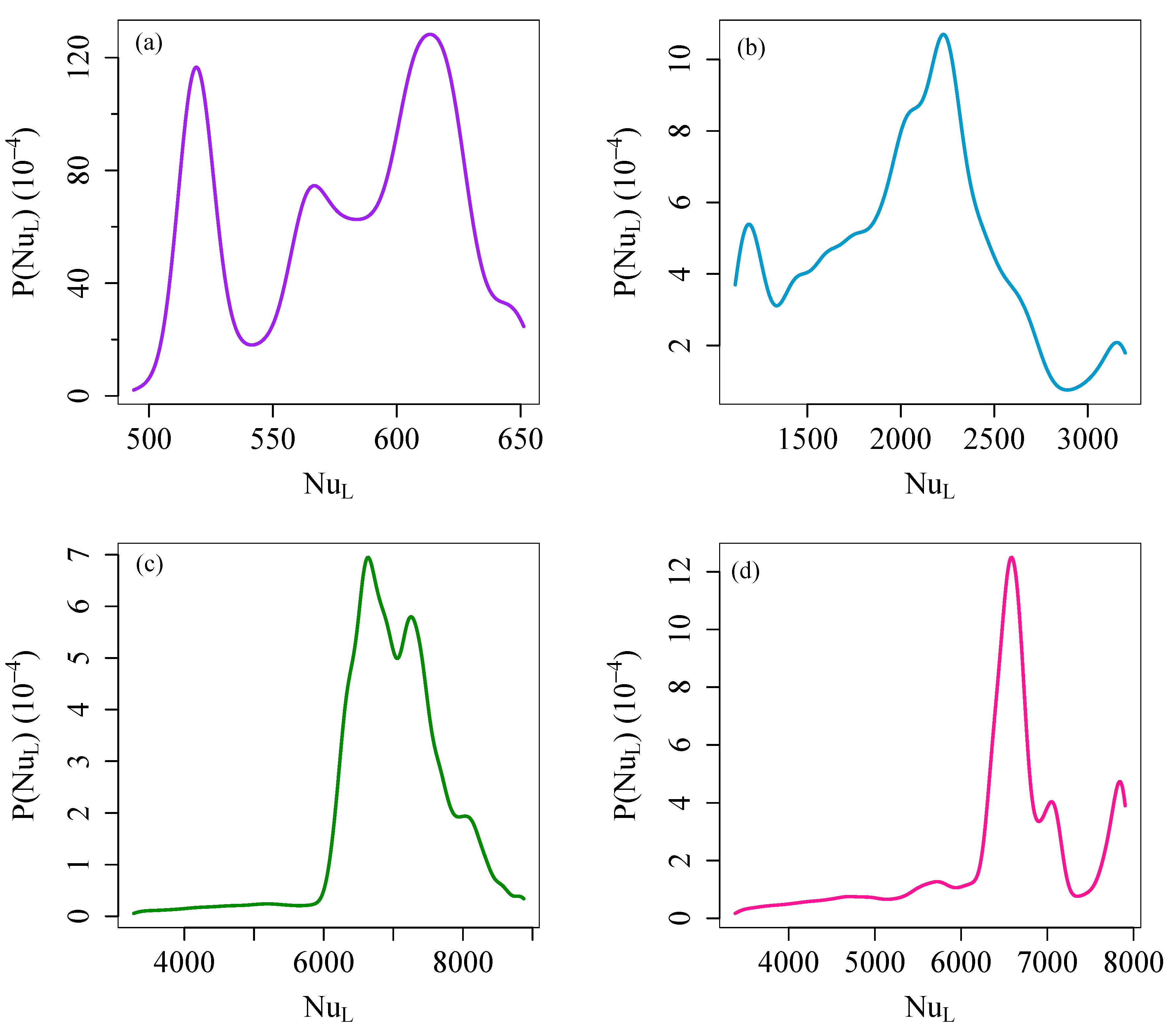
One reason for the inaccuracies in this scaling stems from the use of an average Nusselt number. We find that the instantaneous Nusselt number can change rapidly and vary over a wide range during a simulation of steady state convection, so that neither the average Nusselt number nor its standard deviation characterizes the heat transfer particularly well. Other works have found a similar large time-variation in the Nusselt number, for example see Figure 1 of Schmalzl et al. [28]. To quantify this variation, we examine the probability density functions (PDFs) of the instantaneous Nusselt number from Equation (7) (see Figure 6). In this figure, the PDFs are all multi-modal; two of the four PDFs also feature a heavy tail. To some extent, this may be attributed to the fact that, in our homogeneous system intended to model convection in natural settings, local temperature gradients can become more significant than the imposed and L. Local temperature gradients can also change in time with the changing structure of the flow.
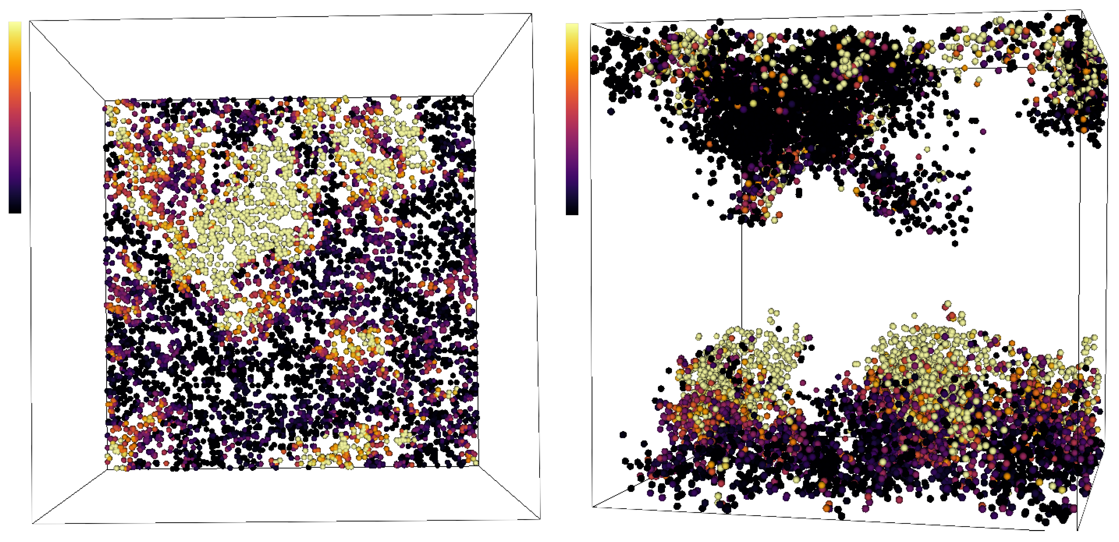
The Nusselt number also varies strongly in space (see Figure 7). Higher values of the Nusselt numbers cluster within coherent flow structures that can be associated with convective plumes. The wide range of Nusselt numbers obtained in these controlled direct numerical simulations makes the definition of an average Nusselt number to characterize the whole flow questionable. We therefore propose a more detailed diagnostic to provide additional information about the heat transport, which we called the Lagrangian heat structure.
4. Results: Lagrangian Heat Structure
4.1. Definition of the Lagrangian Heat Structure
To understand in better detail the transport of heat in convective turbulence and to supplement the information from the average Nusselt number, we define the Lagrangian heat structure. We develop this as an exit-distance statistic, similar in spirit to the finite-time Lyapunov exponent (FTLE) which is used to calculate Lagrangian coherent structures (LCS) [47]. Lagrangian coherent structures have recently been used to clarify length scales for the dynamo [48,49,50]. To calculate the FTLE, a certain finite time is chosen, and the separation of particle pairs is measured after that time is reached. The FTLE of each particle pair is then
In this definition is the separation of the particle pair at the initial time. Rearranging this definition we see that
The FTLE is thus designed to supply a local rate associated with the integrated pair separation.
It is this definition of a rate that can be a useful concept when we adapt it to examine changes in temperature. Instead of a time rate of change, we want to measure an analogous quantity that has units of inverse temperature, and is associated with the diffusion of Lagrangian tracer particles. Rather than emphasize particle pairs, as the FTLE does, we develop a single-particle Lagrangian diagnostic. A possible weakness of employing a single-particle diagnostic rather than a pair diagnostic is that the effect of macroscopic flows can dominate over the small scales. However, since larger scale motions contribute most strongly to heat transport, a single-particle diagnostic seems appropriate to the problem, and has the advantage of also permitting simpler interpretation. In addition, single-particle diagnostics can be averaged over many initial conditions using the conventional methods described in Dubbeldam et al. [51]. This allows these diagnostics to be calculated in a way that is insensitive to the initial conditions of the flow. An investigation of heat transfer might be extended to pair diagnostics in the future.
We construct an equation for the heat in a similar form to Equation (10) so that
We choose a separation in temperature where is the initial temperature that a tracer particle feels. This temperature separation is nondimensional, expressed in units of the root-mean-square of temperature in the system. In Equation (11) we measure the distance that a single particle must diffuse before it achieves that change in temperature in units of the Kolmogorov microscale
Here represents the initial position of the particle. This is a nondimensional construction of distance similar to that used for the diffusion curves in Figure 3. We thus define the Lagrangian heat structure as the ratio
The formulation of Equation (13) as a natural logarithm is useful because it permits the particles that have not yet separated as far as a Kolmogorov microscale to be shown as negative values of .
The Lagrangian heat structure reveals in a local and visual way the positions of particles that experience the fastest change in temperature. We further refine the Lagrangian heat structure in order to isolate only the distance along the mean temperature gradient,
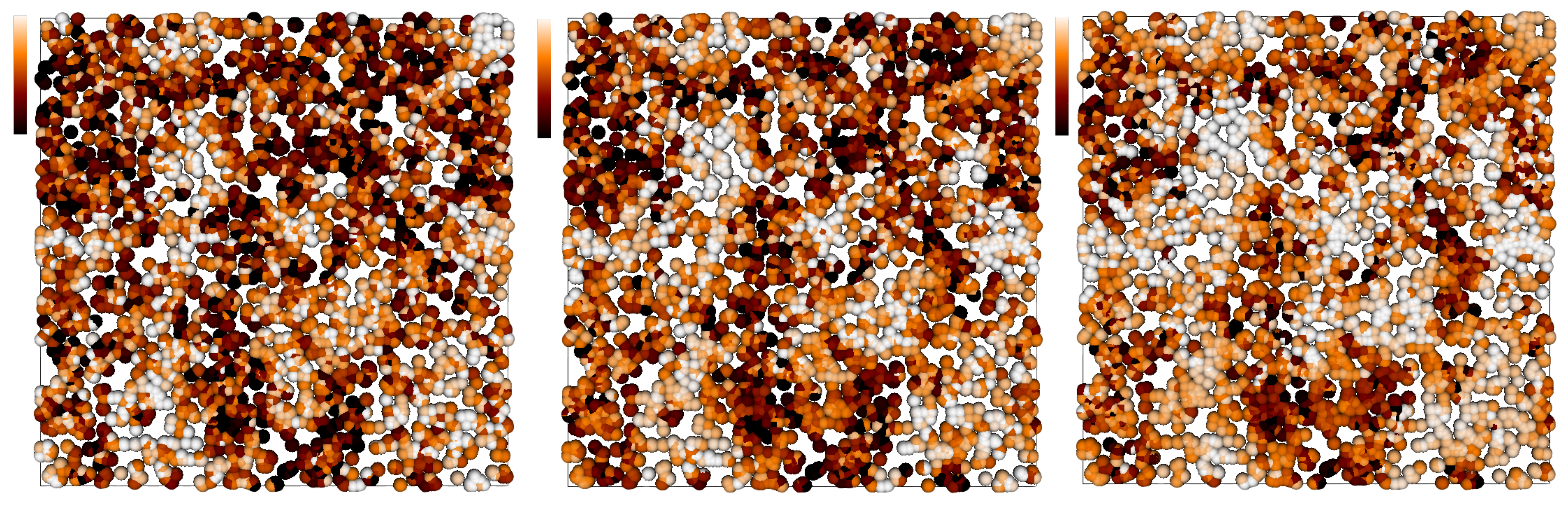
Here the distance used is the distance that the particle moves against gravity, so that . This provides a Lagrangian exit-distance statistic for the transport of heat in the vertical direction. In Figure 8, visualizations show the spatial variation of in a horizontal plane of simulation HC1. The color scale is chosen so that areas of extremely high vertical transport of heat, corresponding to low , are dark. Although the flow is turbulent, clear structures associated with high and low vertical heat transfer are identifiable, and are consistently positioned for different temperature separations. These visualizations may be compared to the visualization of the Nusselt number in Figure 7. The initial time for the calculation of and the horizontal plane are the same as that shown in Figure 7, but the size and position of structures of high vertical transport of heat differ between these figures. In contrast to the instantaneous and rapidly changing Nusselt number, the Lagrangian heat structure represents how changes in heat are connected to an integrated diffusion process. The visualizations in Figure 8 thus reveal more information about the size of structures related to heat transfer in the flow.
4.2. Prandtl Number Dependence of Heat Transfer in Hydrodynamic Convection
For a chosen temperature difference, we calculate the probability density function P and the cumulative distribution function (CDF) C of (see Figure 9). These distributions are calculated for 6 statistically independent flow realizations in simulation HC1. The probability density function deviates from a Gaussian distribution mildly because of the larger lower wing, which is displayed in greater detail by the CDF. We find that this distribution has a shape that changes only slightly for these statistically independent initial points; it does not exhibit the large time intermittency that we observe in the Nusselt number. A similar result is found for each of the other simulations in Table 1. Thus by examining distributions and moments of the Lagrangian vertical heat structure calculated based on all available time data for each simulation, we characterize universally how heat changes in each simulation.
A sample of the cumulative distribution functions for simulations HC1, HC2, and HC3 and several temperature separations are shown in Figure 10. The CDFs we produce are broader for higher Prandtl number, indicating that as the Prandtl number is increased, for more particles, the distance that a particle must diffuse to reach a certain temperature difference is shorter. This result agrees with an intriguing finding of Schmalzl et al. [28] for Rayleigh-Bénard convection. In Figure 8 of that work, the surface area of an arbitrary temperature iso-surface is shown to become smaller with increasing Prandtl number. Since we find that a generally shorter diffusion distance is required to reach a certain temperature difference, our results agree with the finding that the surface area of a temperature iso-surface should be typically smaller in a simulation with larger Prandtl number.
The mean value of the Lagrangian vertical heat structure is shown in panel (a) of Figure 11. When a difference in temperature of is considered, is on average negative for HC3 (); this indicates that this separation in temperature is reached before a particle moves as far as the Kolmogorov microscale. The temperature difference that requires a particle must diffuse further than a Kolmogorov microscale is smaller for simulation HC2 () than HC3 (), and smaller still for simulation HC1 (). This is in agreement with general ideas about flows at different Prandtl number.
As larger differences in temperature are considered, the mean value of appears to approach an asymptotic value that is similar between these simulations. The ordering of the means for different Prandtl numbers agrees with the result of Schmalzl et al. [28] for each . At , the ratio of the mean between HC1 and HC3 is 1.86; between HC2 and HC3 it is 1.27. For these three simulations, for moderately small , the mean Lagrangian vertical heat structure gains a progressively sharper and higher peak as the Prandtl number is decreased. In addition, a comparison between simulations HC2 and HC4 reveals that as the Rayleigh number is increased for fixed Prandtl number, this peak becomes sharper and higher. A comparison between simulations HC1 and HC4 shows that for fixed Grashof number and increasing Prandtl number, the peak becomes less sharp and lower. The results of Figure 11a imply that dynamo simulations that are produced using may represent a transfer of heat that is characteristically similar to the lower Prandtl number settings that they represent, and more accurate for larger heat changes. The standard deviation of is shown in Figure 11b. Surprisingly, unlike the mean, the standard deviation of is nearly identical for all simulations, despite the different Prandtl numbers. The data indicate that this standard deviation decreases approximately as the inverse of the temperature separation.
Higher-order moments can reveal the non-Gaussian character of a process. The skewness and kurtosis are related to the third and fourth moments of a distribution, respectively; their magnitudes are thus a measure of the most basic non-Gaussian aspects. The skewness is defined
Here indicates the expected, or average, value of the quantity in brackets, and m is the mean of x. For a perfectly symmetric distribution the skewness is zero. The form of the kurtosis that we calculate is
This is sometimes also called the excess kurtosis [52], or flatness, and is zero for all univariate Gaussian distributions. The skewness provides a measure of the asymmetry of a distribution, while the kurtosis measures the heaviness of its tails. The skewness and kurtosis of as a function of the temperature separation are shown in Figure 12. The skewness is negative for all temperature separations we calculate, indicating that the left side of the distribution function of is always fatter. This means small values of are more likely than large values, for all obtained in our simulations. For all simulations the skewness shows a characteristic shape with a peak for small values of , followed by a long decay for large values of . For simulation HC1 () this peak is the sharpest, followed by simulation HC2 (), and then simulation HC3 (). The peak for simulation HC4 () is similar to simulation HC2 (). As larger are considered, the skewness becomes more negative, indicating that the distribution of becomes more asymmetric, and small values of become more likely. All three simulations obtain similar values of the skewness for larger temperature separations .
For all simulations the kurtosis of drops sharply for small temperature separations (see Figure 12b). It then grows slowly with increasing . The initial drop is sharpest for HC1 (), followed by simulation HC2 (), and then HC3 (), showing again a clear trend in Prandtl number at fixed Rayleigh number. The drop for simulation HC4 () is slightly more than simulation HC2 (), and slightly less than simulation HC1 (), indicating that the Rayleigh number also plays a role. The higher the kurtosis, the higher the tails of the distribution of relative to the tails of a Gaussian distribution. For moderate and large , the tails of the distributions become more super-Gaussian. However for larger temperature separations , any trend in Prandtl number is lost.
Figure 12 shows that the non-Gaussian aspects of the Lagrangian vertical heat transfer are most dependent on the Prandtl number for small temperature separations . The characteristic shapes produced for the skewness and kurtosis of are universal for all simulations, suggesting that aspects of heat transfer in a low Prandtl number simulation could possibly be captured at moderately higher Prandtl number. The non-zero values of the skewness and kurtosis indicate that any purely Gaussian theory is unlikely to capture important aspects of heat transfer. This supports the similar finding of Emran and Schumacher [53] that PDFs of temperature and its fluctuations are strongly non-Gaussian. Unlike Emran and Schumacher [53], there is no height dependence to the skewness and kurtosis because we examine a homogeneous system.
5. Discussion and Conclusions
After studying the intermittency of the Nusselt number in our simulations of homogeneous turbulent convection, we develop an exit-distance statistic, the Lagrangian heat structure, to quantify properties of heat transfer in a way that is less susceptible to noise and intermittency effects. The Lagrangian heat structure is inspired by the finite-time Lyapunov exponent and the mathematical framework surrounding Lagrangian coherent structures. Local spatial deviations as well as variance in time are easily extracted from the Lagrangian heat structure. This ability to accurately classify extreme variations in a convecting flow is broadly desirable for the study of natural systems. Our new statistic therefore provides a useful supplement to the information provided by the Nusselt number.
We use the Lagrangian vertical heat structure to compare several direct numerical simulations of homogenous turbulent convection at Prandtl numbers 0.1, 1.0, and 10. Different regimes of heat transfer, based on different temperature separations , are revealed by the moments of the distribution of the Lagrangian vertical heat structure. The behavior of the mean, standard deviation, skewness, and kurtosis are characteristically similar for the range of Prandtl numbers studied here. This suggests that a simulation with may be able to reasonably capture qualities of the heat transfer at somewhat larger or smaller Prandtl numbers. This is particularly true if large temperature separations are of primary importance.
This is an encouraging insight for simulations performed with the goal of understanding turbulent convection in natural settings such as Earth’s atmosphere and oceans, as well as planetary and stellar dynamos. Because many numerical studies of the dynamo have been performed at , this observation lends support to the practice of applying these simulation results to realistic natural settings such as a planetary or stellar interior. Our results also indicate that a convecting fluid at room temperature has similarities in the shape of the Lagrangian heat structure to convection in the arctic oceans. If such simulations are performed as large eddy simulations where the smallest scales are modeled rather than resolved, the differences that we note between different Prandtl number simulations at the smallest scales of temperature separation may have even less impact on the simulation results.
This work expands on the findings of several earlier studies of Rayleigh-Bénard convection. Building on the pioneering work of Schumacher [10] to describe convective turbulence from the Lagrangian point of view, we have shown that Lagrangian tracer particles can be used for an exploration of heat transport. Our perspective on heat transport adds to the larger work of Emran and Schumacher [53] that examines the Rayleigh number dependence of higher-order Eulerian statistics of the thermal gradient during turbulent convection. Our development of Lagrangian statistics produces a detailed confirmation of the Eulerian results of Schmalzl et al. [28], particularly the dependence of the iso-surfaces of temperature on the Prandtl number.
Author Contributions
Conceptualization, J.P.; methodology, J.P.; software, J.P., A.B., W.-C.M.; validation, J.P., A.B., W.-C.M., formal analysis, J.P., A.B., W.-C.M.; investigation, J.P., A.B., W.-C.M.; resources, J.P., A.B., W.-C.M.; data curation, J.P.; writing—original draft preparation, J.P., A.B., W.-C.M.; writing—review and editing, J.P., A.B., W.-C.M.; visualization, J.P.; funding acquisition, J.P. All authors have read and agreed to the published version of the manuscript.
Funding
This material is based upon work supported by the US National Science Foundation PHY-1907876. It is also supported by the Thomas Jefferson Fund project entitled “Statistics of turbulent convection.”
Acknowledgments
This work used the ARCHER UK National Supercomputing Service (http://www.archer.ac.uk) as part of the UK Turbulence Consortium. This work has been supported by the Engineering and Physical Sciences Research Council Grants No. EP/L000261/1. Additional calculations were performed on the Konrad and Gottfried computer systems of the Norddeutsche Verbund zur Förderung des Hoch- und Höchstleistungsrechnens (HLRN) by the project bep00051 “Lagrangian studies of incompressible turbulence in plasmas”. Calculations were performed on the Cluster-I of the Technical University of Berlin, and the University of Exeter Supercomputer, a DiRAC Facility jointly funded by STFC, the Large Facilities Capital Fund of BIS and the University of Exeter.
Conflicts of Interest
The authors declare no conflict of interest. The funders had no role in the design of the study; in the collection, analyses, or interpretation of data; in the writing of the manuscript, or in the decision to publish the results.
References
- Gifford, F., Jr. Relative Atmospheric Diffusion of Smoke Puffs. J. Atmos. Sci. 1957, 14, 410–414. [Google Scholar] [CrossRef] [Green Version]
- Roberts, O. The theoretical scattering of smoke in a turbulent atmosphere. Proc. R. Soc. A-Math. Phys. 1923, 104, 640–654. [Google Scholar]
- Sutton, O.G. A theory of eddy diffusion in the atmosphere. Proc. R. Soc. A-Math. Phys. 1932, 135, 143–165. [Google Scholar]
- Frenkiel, F.; Katz, I. Studies of small-scale turbulent diffusion in the atmosphere. J. Meteorol. 1956, 13, 388–394. [Google Scholar] [CrossRef]
- Kellogg, W.W. Diffusion of smoke in the stratosphere. J. Meteorol. 1956, 13, 241–250. [Google Scholar] [CrossRef] [Green Version]
- Yeung, P. Lagrangian investigations of turbulence. Annu. Rev. Fluid Mech. 2002, 34, 115–142. [Google Scholar] [CrossRef]
- Toschi, F.; Bodenschatz, E. Lagrangian properties of particles in turbulence. Annu. Rev. Fluid Mech. 2009, 41, 375–404. [Google Scholar] [CrossRef]
- Gasteuil, Y.; Shew, W.L.; Gibert, M.; Chilla, F.; Castaing, B.; Pinton, J.F. Lagrangian temperature, velocity, and local heat flux measurement in Rayleigh-Bénard convection. Phys. Rev. Lett. 2007, 99, 234302. [Google Scholar] [CrossRef] [Green Version]
- Schumacher, J. Lagrangian dispersion and heat transport in convective turbulence. Phys. Rev. Lett. 2008, 100, 134502. [Google Scholar] [CrossRef] [Green Version]
- Schumacher, J. Lagrangian studies in convective turbulence. Phys. Rev. E 2009, 79, 056301. [Google Scholar] [CrossRef]
- Emran, M.S.; Schumacher, J. Lagrangian tracer dynamics in a closed cylindrical turbulent convection cell. Phys. Rev. E 2010, 82, 016303. [Google Scholar] [CrossRef] [Green Version]
- Schütz, S.; Bodenschatz, E. Two-particle dispersion in weakly turbulent thermal convection. New J. Phys. 2016, 18, 065007. [Google Scholar] [CrossRef] [Green Version]
- Liot, O.; Seychelles, F.; Zonta, F.; Chibbaro, S.; Coudarchet, T.; Gasteuil, Y.; Pinton, J.F.; Salort, J.; Chillà, F. Simultaneous temperature and velocity Lagrangian measurements in turbulent thermal convection. J. Fluid Mech. 2016, 794, 655–675. [Google Scholar] [CrossRef] [Green Version]
- Boffetta, G.; Sokolov, I. Statistics of two-particle dispersion in two-dimensional turbulence. Phys. Fluids 2002, 14, 3224–3232. [Google Scholar] [CrossRef] [Green Version]
- Aurell, E.; Boffetta, G.; Crisanti, A.; Paladin, G.; Vulpiani, A. Predictability in the large: An extension of the concept of Lyapunov exponent. J. Phys. A 1997, 30, 1. [Google Scholar] [CrossRef] [Green Version]
- Bettencourt, J.H.; López, C.; Hernández-García, E. Characterization of coherent structures in three-dimensional turbulent flows using the finite-size Lyapunov exponent. J. Phys. A 2013, 46, 254022. [Google Scholar] [CrossRef]
- Karrasch, D.; Haller, G. Do Finite-Size Lyapunov Exponents Detect Coherent Structures? Chaos 2013, 23, 043126. [Google Scholar] [CrossRef] [Green Version]
- Salazar, J.P.; Collins, L.R. Two-particle dispersion in isotropic turbulent flows. Annu. Rev. Fluid Mech. 2009, 41, 405–432. [Google Scholar] [CrossRef] [Green Version]
- Biferale, L.; Cencini, M.; Vergni, D.; Vulpiani, A. Exit time of turbulent signals: A way to detect the intermediate dissipative range. Phys. Rev. E 1999, 60, R6295. [Google Scholar] [CrossRef] [Green Version]
- Biferale, L.; Cencini, M.; Lanotte, A.S.; Vergni, D. Inverse velocity statistics in two-dimensional turbulence. Phys. Fluids 2003, 15, 1012–1020. [Google Scholar] [CrossRef] [Green Version]
- LaCasce, J. Lagrangian statistics from oceanic and atmospheric observations. In Transport and Mixing in Geophysical Flows; Springer: Berlin/Heidelberg, Germany, 2008; pp. 165–218. [Google Scholar]
- Shew, W.L.; Gasteuil, Y.; Gibert, M.; Metz, P.; Pinton, J.F. Instrumented tracer for Lagrangian measurements in Rayleigh-Bénard convection. Rev. Sci. Instrum. 2007, 78, 065105. [Google Scholar] [CrossRef] [Green Version]
- Vassilicos, J.C. Intermittency in Turbulent Flows; Cambridge University Press: Cambridge, UK, 2001. [Google Scholar]
- Feraco, F.; Marino, R.; Pumir, A.; Primavera, L.; Mininni, P.D.; Pouquet, A.; Rosenberg, D. Vertical drafts and mixing in stratified turbulence: Sharp transition with Froude number. EPL 2018, 123, 44002. [Google Scholar] [CrossRef] [Green Version]
- Boffetta, G.; Sokolov, I. Relative dispersion in fully developed turbulence: The Richardson?s law and intermittency corrections. Phys. Rev. Lett. 2002, 88, 094501. [Google Scholar] [CrossRef] [Green Version]
- He, X.; Funfschilling, D.; Nobach, H.; Bodenschatz, E.; Ahlers, G. Transition to the ultimate state of turbulent Rayleigh-Bénard convection. Phys. Rev. Lett. 2012, 108, 024502. [Google Scholar] [CrossRef] [Green Version]
- Stevens, R.J.; Lohse, D.; Verzicco, R. Prandtl and Rayleigh number dependence of heat transport in high Rayleigh number thermal convection. J. Fluid Mech. 2011, 688, 31–43. [Google Scholar] [CrossRef] [Green Version]
- Schmalzl, J.; Breuer, M.; Hansen, U. The influence of the Prandtl number on the style of vigorous thermal convection. Geophys. Astrophys. Fluid 2002, 96, 381–403. [Google Scholar] [CrossRef]
- Schumacher, J.; Götzfried, P.; Scheel, J.D. Enhanced enstrophy generation for turbulent convection in low-Prandtl-number fluids. Proc. Natl. Acad. Sci. USA 2015, 122, 9530–9535. [Google Scholar] [CrossRef] [Green Version]
- Petschel, K.; Stellmach, S.; Wilczek, M.; Lülff, J.; Hansen, U. Kinetic energy transport in Rayleigh–Bénard convection. J. Fluid Mech. 2015, 773, 395–417. [Google Scholar] [CrossRef] [Green Version]
- Williamson, J.H. Low-storage Runge-Kutta schemes. J. Comput. Phys. 1980, 35, 48–56. [Google Scholar] [CrossRef]
- Calzavarini, E.; Lohse, D.; Toschi, F.; Tripiccione, R. Rayleigh and Prandtl number scaling in the bulk of Rayleigh-Bénard turbulence. Phys. Fluids 2005, 17, 055107. [Google Scholar] [CrossRef] [Green Version]
- Pratt, J.; Busse, A.; Müller, W.C. Fluctuation dynamo amplified by intermittent shear bursts in convectively driven magnetohydrodynamic turbulence. Astron. Astrophys. 2013, 557, A76. [Google Scholar] [CrossRef]
- Pratt, J.; Busse, A.; Mueller, W.C.; Chapman, S.; Watkins, N. Anomalous dispersion of Lagrangian particles in local regions of turbulent flows revealed by convex hull analysis. arXiv 2014, arXiv:1408.5706. [Google Scholar]
- Pratt, J.; Busse, A.; Müller, W.; Watkins, N.; Chapman, S.C. Extreme-value statistics from Lagrangian convex hull analysis for homogeneous turbulent Boussinesq convection and MHD convection. New J. Phys. 2017, 19, 065006. [Google Scholar] [CrossRef] [Green Version]
- Gibert, M.; Pabiou, H.; Chilla, F.; Castaing, B. High-Rayleigh-number convection in a vertical channel. Phys. Rev. Lett. 2006, 96, 084501. [Google Scholar] [CrossRef] [Green Version]
- Pope, S.B. Turbulent Flows; Cambridge University Press: Cambridge, UK, 2000. [Google Scholar]
- Grötzbach, G. Spatial resolution requirements for direct numerical simulation of the Rayleigh-Bénard convection. J. Comput. Phys. 1983, 49, 241–264. [Google Scholar] [CrossRef]
- Kaczorowski, M.; Wagner, C. Study on the resolution requirements for DNS in turbulent Rayleigh-Bénard convection. In Turbulence and Interactions; Springer: Berlin/Heidelberg, Germany, 2010; pp. 199–205. [Google Scholar]
- Homann, H.; Dreher, J.; Grauer, R. Impact of the floating-point precision and interpolation scheme on the results of DNS of turbulence by pseudo-spectral codes. Comput. Phys. Commun. 2007, 177, 560–565. [Google Scholar] [CrossRef] [Green Version]
- Busse, A.; Müller, W.C. Diffusion and dispersion in magnetohydrodynamic turbulence: The influence of mean magnetic fields. Astron. Nachrichten Astron. Notes 2008, 329, 714–716. [Google Scholar] [CrossRef]
- Buaria, D.; Pumir, A.; Feraco, F.; Marino, R.; Pouquet, A.; Rosenberg, D.; Primavera, L. Single-particle Lagrangian statistics from direct numerical simulations of rotating-stratified turbulence. Phys. Rev. Fluids 2020, 5, 064801. [Google Scholar] [CrossRef]
- Niemela, J. Static and dynamic measurements of the Nusselt number in turbulent convection. Phys. Scr. 2013, 2013, 014059. [Google Scholar] [CrossRef]
- Stevens, R.J.; Verzicco, R.; Lohse, D. Radial boundary layer structure and Nusselt number in Rayleigh–Bénard convection. J. Fluid Mech. 2010, 643, 495–507. [Google Scholar] [CrossRef] [Green Version]
- Grossmann, S.; Lohse, D. Scaling in thermal convection: A unifying theory. J. Fluid Mech. 2000, 407, 27–56. [Google Scholar] [CrossRef] [Green Version]
- Chillà, F.; Schumacher, J. New perspectives in turbulent Rayleigh-Bénard convection. Eur. Phys. J. E Soft Matter 2012, 35, 1–25. [Google Scholar] [CrossRef] [PubMed] [Green Version]
- Haller, G. Lagrangian coherent structures. Annu. Rev. Fluid Mech. 2015, 47, 137–162. [Google Scholar] [CrossRef] [Green Version]
- Rempel, E.L.; Chian, A.L.; Brandenburg, A. Lagrangian coherent structures in nonlinear dynamos. Astrophys. J. Lett. 2011, 735, L9. [Google Scholar] [CrossRef]
- Rempel, E.L.; Chian, A.C.; Brandenburg, A. Lagrangian chaos in an ABC-forced nonlinear dynamo. Phys. Scr. 2012, 86, 018405. [Google Scholar] [CrossRef] [Green Version]
- Rempel, E.L.; Chian, A.C.L.; Brandenburg, A.; Muñoz, P.R.; Shadden, S.C. Coherent structures and the saturation of a nonlinear dynamo. J. Fluid Mech. 2013, 729, 309–329. [Google Scholar] [CrossRef] [Green Version]
- Dubbeldam, D.; Ford, D.C.; Ellis, D.E.; Snurr, R.Q. A new perspective on the order-n algorithm for computing correlation functions. Mol. Simul. 2009, 35, 1084–1097. [Google Scholar] [CrossRef] [Green Version]
- Abramowitz, M.; Stegun, I. Handbook of Mathematical Functions, 9th ed.; U.S. Government Printing Office: Washington, DC, USA, 1970.
- Emran, M.; Schumacher, J. Fine-scale statistics of temperature and its derivatives in convective turbulence. J. Fluid Mech. 2008, 611, 13–34. [Google Scholar] [CrossRef] [Green Version]
Figure 1.
Visualization of thermal energy in simulation HC4 described in Table 1. The physical set-up of the simulations is also indicated.
Figure 1.
Visualization of thermal energy in simulation HC4 described in Table 1. The physical set-up of the simulations is also indicated.

Figure 2.
Kinetic energy spectrum (a) and thermal energy spectrum (b) for simulations HC1, HC2, HC3, and HC4.
Figure 2.
Kinetic energy spectrum (a) and thermal energy spectrum (b) for simulations HC1, HC2, HC3, and HC4.

Figure 3.
Lagrangian single-particle diffusion curves in the direction (a) parallel to gravity, and (b) perpendicular to gravity for simulations HC1, HC2, HC3, and HC4. Time is given in units of the Kolmogorov time-scale .
Figure 3.
Lagrangian single-particle diffusion curves in the direction (a) parallel to gravity, and (b) perpendicular to gravity for simulations HC1, HC2, HC3, and HC4. Time is given in units of the Kolmogorov time-scale .

Figure 4.
Lagrangian autocorrelation function of (a) the velocity aligned with gravity , and (b) the thermal fluctuations . In (b) a dotted grey line is provided in the background as a reference for the autocorrelation function of in the simulation HC2. Time is given in units of the Kolmogorov time-scale . Triangular brackets indicate an average over Lagrangian particles.

Figure 5.
The scaling of the Nusselt number with the product of Prandtl and Rayleigh numbers. The shaded region indicates one standard deviation of the instantaneous Nusselt number above and below the time-averaged value.
Figure 5.
The scaling of the Nusselt number with the product of Prandtl and Rayleigh numbers. The shaded region indicates one standard deviation of the instantaneous Nusselt number above and below the time-averaged value.

Figure 6.
Probability density functions of the instantaneous Nusselt number for (a) simulation HC1 (), (b) simulation HC2 (), (c) simulation HC3 (), and (d) simulation HC4 ().
Figure 6.
Probability density functions of the instantaneous Nusselt number for (a) simulation HC1 (), (b) simulation HC2 (), (c) simulation HC3 (), and (d) simulation HC4 ().

Figure 7.
Visualization of particles in a slice of the simulation volume determined by the first three grid spaces in the z-direction in simulation HC1: two-dimensional visualization at the initial time point (left), and three dimensional visualization as the same particles trace the evolution of the evolving convective flow structures (right). Particles are colored by the instantaneous local Nusselt number that they experience between zero and , with dark colors indicating a low Nusselt number and bright colors indicating a high Nusselt number.

Figure 8.
Visualizations of the Lagrangian vertical heat structure in the same slice of the simulation volume shown in Figure 7, in simulation HC1 () for temperature separations (left), (middle), and (right). Darker color indicates a lower value of .
Figure 8.
Visualizations of the Lagrangian vertical heat structure in the same slice of the simulation volume shown in Figure 7, in simulation HC1 () for temperature separations (left), (middle), and (right). Darker color indicates a lower value of .

Figure 9.
Distribution functions of the Lagrangian vertical heat structure for , constructed from approximately 4 million Lagrangian tracer particles in simulation HC1 (). (a) Probability density function constructed from the data for 6 different statistically independent flow realizations. (b) Cumulative distribution function. Six dashed lines show distributions constructed from data at different independent flow realizations; the solid line represents a distribution constructed from the data at all 6 times. A dotted line marks the point where .

Figure 10.
Cumulative distribution function of the Lagrangian vertical heat structure for (a) a temperature separation of in simulations HC1 (), HC2 (), and HC3 (), and (b) for a range of temperature separations in simulation HC1. A dotted line marks the point where . Distributions are constructed from approximately 4 million Lagrangian tracer particles, sampled for 6 different statistically independent flow realizations.

Figure 11.
Mean (a) and standard deviation (b) of for simulations HC1, HC2, HC3, and HC4.

Figure 12.
Skewness (a) and kurtosis (b) of vs. temperature separation for simulations HC1, HC2, HC3, and HC4.
Figure 12.
Skewness (a) and kurtosis (b) of vs. temperature separation for simulations HC1, HC2, HC3, and HC4.


Table 1.
Parameters of homogeneous hydrodynamic convection simulations. The simulations are defined by the value of the Rayleigh number, calculated according to Section 2.2, and the Prandtl number. The Nusselt number is calculated according to Equation (7). The Grashof number is defined . The nondimensionalized kinematic viscosity and the thermal diffusivity are also provided.
| Simulation | HC1 | HC2 | HC3 | HC4 |
|---|---|---|---|---|
| grid size | ||||
| simulation time () | 484 | 1605 | 416 | 427 |
| () | 4 | 4 | 4 | 8 |
| Prandtl number | 0.1 | 1.0 | 10 | 1.0 |
| Rayleigh number | ||||
| Grashof number | ||||
| Reynolds number | 3230 | 1350 | 570 | 4180 |
| Nusselt no. | 582 | 2025 | 6980 | 6503 |
| time maximum of | 651 | 3200 | 8873 | 7903 |
| () | 3.43 | 7.60 | 17.0 | 3.23 |
| () | 1.85 | 5.03 | 4.57 | 1.64 |
| () | 1.92 | 7.57 | 3.01 | 3.24 |
| () | 10.18 | 2.21 | 2.52 | 2.86 |
© 2020 by the authors. Licensee MDPI, Basel, Switzerland. This article is an open access article distributed under the terms and conditions of the Creative Commons Attribution (CC BY) license (http://creativecommons.org/licenses/by/4.0/).
Share and Cite
MDPI and ACS Style
Pratt, J.; Busse, A.; Müller, W.-C. Lagrangian Statistics of Heat Transfer in Homogeneous Turbulence Driven by Boussinesq Convection. Fluids 2020, 5, 127. https://doi.org/10.3390/fluids5030127
AMA Style
Pratt J, Busse A, Müller W-C. Lagrangian Statistics of Heat Transfer in Homogeneous Turbulence Driven by Boussinesq Convection. Fluids. 2020; 5(3):127. https://doi.org/10.3390/fluids5030127
Chicago/Turabian StylePratt, Jane, Angela Busse, and Wolf-Christian Müller. 2020. "Lagrangian Statistics of Heat Transfer in Homogeneous Turbulence Driven by Boussinesq Convection" Fluids 5, no. 3: 127. https://doi.org/10.3390/fluids5030127