Jet Oscillation Frequency Characterization of a Sweeping Jet Actuator †


School of Mechanical and Aerospace Engineering, Oklahoma State University, Stillwater, OK 74078, USA
*
Author to whom correspondence should be addressed.
†
This paper is an extended version of our paper “Numerical Simulation of a Sweeping Jet Actuator” published at the 34th AIAA Applied Aerodynamics Conference, AIAA AVIATION Forum, Washington, DC, USA, 13–17 June 2016.
Fluids 2020, 5(2), 72; https://doi.org/10.3390/fluids5020072
Submission received: 28 February 2020
/
Revised: 8 May 2020
/
Accepted: 12 May 2020
/
Published: 14 May 2020
(This article belongs to the Special Issue Recent Numerical Advances in Fluid Mechanics, Volume II)
Abstract
:The time-resolved flow field of a spatially oscillating jet emitted by a sweeping jet (SWJ) actuator is investigated numerically using three-dimensional Reynolds-averaged Navier–Stokes (3D-URANS) equations. Numerical simulations are performed for a range of mass flow rates providing flow conditions varying from incompressible to subsonic compressible flows. After a detailed mesh study, the computational domain is represented using two million hexagonal control volumes. The jet oscillation frequency is predicted by analyzing velocity time histories at the actuator exit, and a linear relationship between the jet oscillation frequency and time-averaged exit nozzle Mach number is found (, R² = 0.97). The results of our numerical model are compared with data from the literature, and a good agreement is found. In addition, we confirmed that the Strouhal number is almost constant with the Mach number for the subsonic oscillating jet and has an average value of St = 0.0131. The 3D-URANS model that we presented here provides a computationally inexpensive yet accurate alternative to the researchers to investigate jet oscillation characteristics.
1. Introduction
Active flow control (AFC) has been a popular research topic since its discovery in the 1950s. In earlier applications, research was mainly focused on reducing takeoff and landing speeds of military aircraft. The development and application of AFC technologies for commercial platforms accelerated in the 2000s, and several programs were initiated. For example, the National Aeronautics and Space Administration (NASA) Environmentally Responsible Aviation (ERA) project was focused on developing technologies to reduce noise level and fuel consumption of future aircraft by employing AFC technology [1]. Boeing’s ecoDemonstrator 757 [2] is another example of utilizing AFC via a sweeping jet (SWJ) actuator in commercial platforms to enhance the aerodynamic efficiency of a vertical tail [3].
Fluidic actuators employed in AFC increase the momentum of the local flow field by fluid injection or suction. The SWJ actuator is a fluidic actuator. It generates a self-induced self-sustaining oscillating jet flow field due to its interior geometric design, feedback channels, and mixing chamber, as shown in Figure 1. Historically, SWJ actuators are employed in many applications, such as windshield-washer fluid nozzles [4] and flow-metering devices [5,6]. Recently, SWJ actuators have been explored in several numerical and experimental studies [7,8,9,10,11,12,13,14,15,16,17,18,19,20,21,22,23,24,25,26,27,28,29,30,31,32,33,34,35]. Aerodynamic performance was reported to improve by up to 60% in active flow control studies, namely a single-element high-lift airfoil [36], a V-22 wing-nacelle combination [37], and wind turbine blades [38]. The SWJ actuators successfully reduced the drag force on trucks [39] and bluff bodies [40] and suppressed the flow separation bubble [41]. Moreover, the side force was increased by 50–70% on a typical twin-engine aircraft whose vertical tail has multiple SWJ actuators operating at Reynolds numbers up to 1.5 million [42].
In the last decade, there has been a significant increase in the utilization of SWJ actuators for AFC projects. The SWJ actuator’s flow physics, design parameters, and working principles have been investigated numerically and experimentally. In a recent experimental study conducted at the NASA Langley 15-inch low-speed tunnel, several actuator parameters were investigated, including blowing coefficients, operation mode, pitch and spreading angles, and actuator size [43]. The results indicate that the SWJ actuators were more effective than other well-known flow control techniques such as steady blowing and steady vortex-generating jets. Internal dynamics of SWJ actuators were investigated using a high-speed camera, and two different SWJ actuators were characterized based on their jet oscillation frequency and mass flow rate [44]. The jet oscillation process was shown in detail at 650 Hz and 1250 Hz. The results showed the effect of compressibility on the oscillation frequency and deviation from the linear trend line. In another study, the high-frequency characterization of an SWJ actuator was performed experimentally above 500 Hz [45]. The acoustic field of SWJ actuators also measured at full- and half-scale [46]. The findings suggested that rougher internal surfaces with 3D printed actuators resulted in higher sweep frequency. Moreover, the effects of SWJ actuator geometry on the jet oscillation frequency was studied numerically for incompressible flows [47]. The authors confirmed that the effect of feedback channel length on the oscillation frequency is negligible. However, the results showed that a longer mixing chamber reduced the jet oscillation frequency.
The objective of this study is to investigate the effects of inflow mass flow rate and compressibility on the jet oscillation frequency of the SWJ actuator. Time-averaged velocities at various streamwise and spanwise locations will be presented. For some selected cases, the time history of velocities sampled at the SWJ outlet and frequency analysis will be provided and discussed. A correlation function will be recommended to predict jet oscillation frequency.
2. Numerical Methodology
In this section, we present the numerical model used to obtain the SWJ actuator oscillation frequency for several inflow mass flow rates. The Favre-averaged Navier–Stokes equations for the conservation of mass, momentum, and energy for compressible flows are written below. The interested reader should refer to the additional references [48,49,50] for detailed derivations.
where are the spatial coordinates, are velocity components; is the pressure; and are the density and temperature of the fluid, respectively. The heat flux vector is obtained from Fourier’s law and where is the thermal conductivity. The Favre-averaged heat flux vector and Reynolds-stress tensor are and , respectively. The total energy and total enthalpy, including the kinetic energy of the fluctuating turbulent field, are and , respectively. Favre-averaged turbulent kinetic energy is defined as . We assumed calorically perfect gas and thus the specific internal energy, , and specific enthalpy, , are and where and are the specific-heat coefficients for constant volume and pressure processes, respectively.
In the Reynolds averaging procedure, we write an instantaneous variable, , as the sum of mean, , and fluctuating, , parts, i.e., . On the other hand, in the Favre averaging, it is customary to decompose the instantaneous variable, , into the mass-averaged part, , and a fluctuating part, as . In the governing equations, the overbar indicates Reynolds average (time average), and the tilda represents the Favre average (density-weighted average): .
In the simulations, the working fluid is air, and the Prandtl number is 0.72. The molecular viscosity is evaluated using Sutherland’s law:
where the reference viscosity kg m−1 s−1, reference temperature K, and effective temperature K.
The governing equations are solved using ANSYS Fluent (version 17.1) [52]. It employs a control volume method to discretize the Reynolds-averaged Navier–Stokes (RANS) equations with second-order accuracy. The pressure-implicit with splitting of operators (PISO) algorithm is used for unsteady calculations with a second order fully implicit scheme for time integration. Numerical simulations are initialized using the inlet boundary conditions provided in Table 1, where static pressure and temperature are 101,325 Pa and 298.16 K, respectively. Inlet velocity is calculated using the equation where density and area at the inlet are 1.184 kg/m3 and 102.93 mm2. A uniform velocity distribution is assumed at the initial stage.
The geometry of the SWJ actuator is similar to the previous computational and experimental studies [9,17,41,53]. The schematic of the actuator and the three-dimensional (3D) computational domain is presented in Figure 1, and the CAD model is provided in the Supplementary Materials. In the computational domain, the x-axis corresponds to the streamwise direction, the y-axis corresponds to the spanwise direction, and z-axis corresponds to the vertical direction. The computational domain is symmetric about the x-axis and the XY-plane. The origin is located at the cross-section of the x-axis and SWJ actuator exit wall plane, as shown in Figure 1. The SWJ actuator has a mixing chamber, an exit nozzle to the outlet, and two feedback channels. The exit nozzle throat size, h, is chosen as a length scale. The actuator depth, d, is constant and equal to the h. In the present study, the aspect ratio (h/d) of the exit nozzle throat is 1, where h = 6.35 mm. The area ration of the inlet to the exit nozzle throat is 2.5531. The width of the feedback channel and the mixing chamber are 7.43 mm and 21.52 mm, respectively.
For unsteady analyses, we adopted a constant time step size is set to Δt = 1 × 10⁻⁵ s based on our previous study [41]. As a result, a jet oscillation cycle for the highest mass flow rate ( = 11.3398 g/s) can be captured with 210 time-steps. The solution does not change with a further reduction of the time step. Previous studies documented that increasing the mass flow rate increases the jet oscillation frequency [9,53], and therefore, the same time-step size is used in all simulations.
To obtain a fully developed oscillating jet, each computation is initialized with a constant mass flow rate at the inlet boundary, and an unsteady simulation is run for 10,000 time-steps (0.1 s, or approximately 50 periods for = 11.3398 kg/s). For each time step, 20 Newton sub-iterations are performed for temporal convergence. Next, the unsteady simulation is run for another 10,000 time-steps to record time statistics. As a result, 20,000 time-steps or 0.2 s is simulated for each case.
The computational mesh is created using the Ansys Meshing software by employing hexagonal mesh elements. Figure 2 shows the computational mesh. The element size is determined based on the characteristic length, h. The boundary layer is resolved using 25 layers in the wall-normal direction with a growth rate of 1.1, as presented in the reference [41]. The first point of the wall is placed at h/500 (0.0127 mm) in the wall-normal direction. The y+ values of the resulting mesh are less than one. To generate the coarse mesh, the element size inside the actuator is assumed to be h/10, and the resulting mesh has 60 elements across the exit throat nozzle, including 25 elements for each wall and ten elements to fill the space between the boundary layer meshes. This mesh is named N10, referring to the number of elements (N = 10) to fill the space between the boundary layer meshes. The element size in the z-direction is assumed to be h/10.
To control the element size, two levels of refinement are applied using the sphere of influence method with sphere radii of 8h and 20h. The maximum element size for the outer sphere is set to N5. For the inner sphere, the element size can be changed from N10 to N80. To perform mesh sensitivity analysis, the number of elements is successively increased, and four different meshes are created resulting in coarse, normal, fine, and finest meshes. The mesh parameters are given in Table 2. The finest mesh (N80) has 130 elements across the exit nozzle throat, and the resulting mesh has 6.7 million elements. We evaluated the sensitivity of numerical calculations to the mesh size given in Table 2 by employing the numerical model described above to determine adequate mesh resolution. The results of the mesh sensitivity analysis are presented in the next section.
3. Results
3.1. Mesh Sensitivity Analysis
Performing a mesh sensitivity analysis is critically important to minimize spatial discretization errors and computational cost. In this study, four different meshes are employed, and their parameters are presented in Table 2. The coarse mesh (N10) has approximately 0.4 million elements, and the finest mesh (N80) has approximately 6.7 million elements. Using the numerical model described in the previous section, a set of time-accurate simulations are performed using a mass flow rate of 6.8039 g/s for all the meshes listed in Table 2.
The time-averaged velocity profile along the SWJ actuator symmetry line (x-axis) is presented in Figure 3. In the figure, the velocity is non-dimensionalized by the maximum velocity at the SWJ actuator exit nozzle throat. The peak velocity of the finest mesh (N80) is 172.7 m/s. The coarse mesh (N10) result at the same location has a 1.9% deviation (3.3 m/s), as shown in Figure 3b. There is no discernible difference between the results of N40 and N80, indicating that the independent mesh results are obtained for the mesh N40. Moreover, time-averaged static pressure and temperature profiles along the symmetry line are presented in Figure 4. The results are non-dimensionalized with free stream values, e.g., P∞ = 101,325 Pa and T∞ = 288.16 K. The pressure and temperature profiles converge to N80 results with increased mesh resolution. There is no visible difference in the results between N40 and N80 meshes.
Time-averaged velocity contours are compared for the coarse and the finest meshes in Figure 5. For an easy comparison, the same contour levels are used in the figures. Figure 5a shows that the flow velocity in the feedback channel and actuator inlet are overpredicted, but at the exit nozzle, it was underpredicted in the coarse mesh simulation.
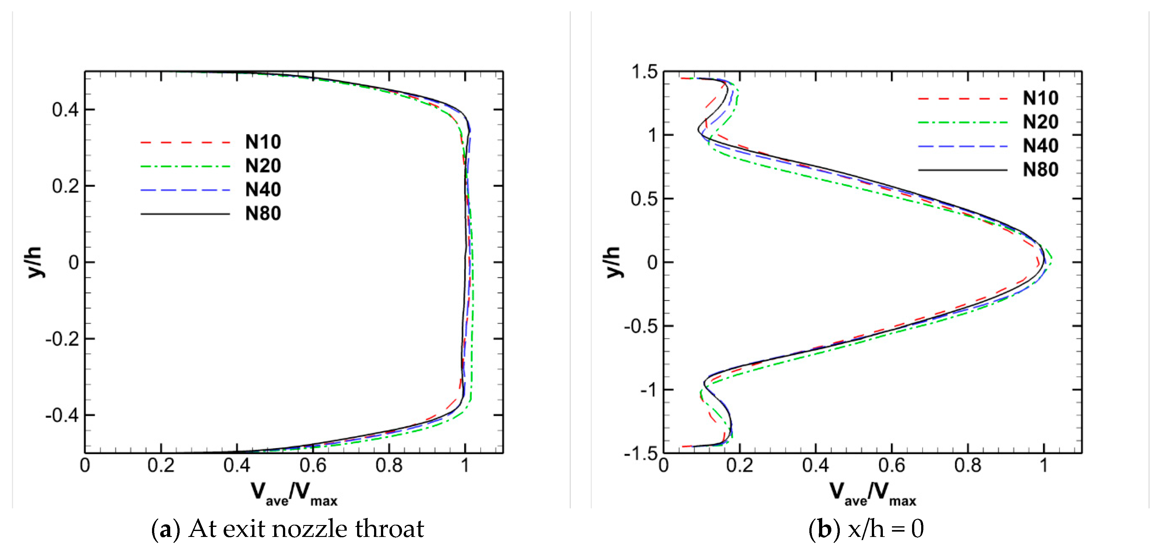
To perform a detailed comparison, velocity profiles are plotted at various downstream locations in Figure 6. At the SWJ exit nozzle throat, all the results follow the same trend. However, the coarse and normal mesh profiles deviate from the fine mesh results. The coarse mesh simulation underestimates velocity at y/h = ±0.35 locations. The simulation using the normal mesh underestimates the velocity at y/h = 0.35 but slightly overestimates elsewhere. The differences among the velocity profiles become clearer at further downstream locations, as shown in Figure 6b–d. The double velocity peak is only visible in the fine and very fine meshes. The velocity profile of normal mesh (N20) shifted for all locations. The coarse mesh (N10) and normal mesh (N20) fail to capture the peak velocity, jet width, and direction. Although simulations are run for 34 periods of jet oscillation (10,000 time-steps with Δt = 1 × 10⁻⁵ s) the time-averaged velocity profiles are not entirely symmetric even in the case of the finest grid as shown in Figure 6d. A longer simulation might result in better converged time statistics. Up to this point, we compared the time-averaged results for various mesh resolutions and found that the fine mesh (N40) can capture the time-averaged flow quantities. In the next paragraph, comparisons for time-accurate simulations will be presented.
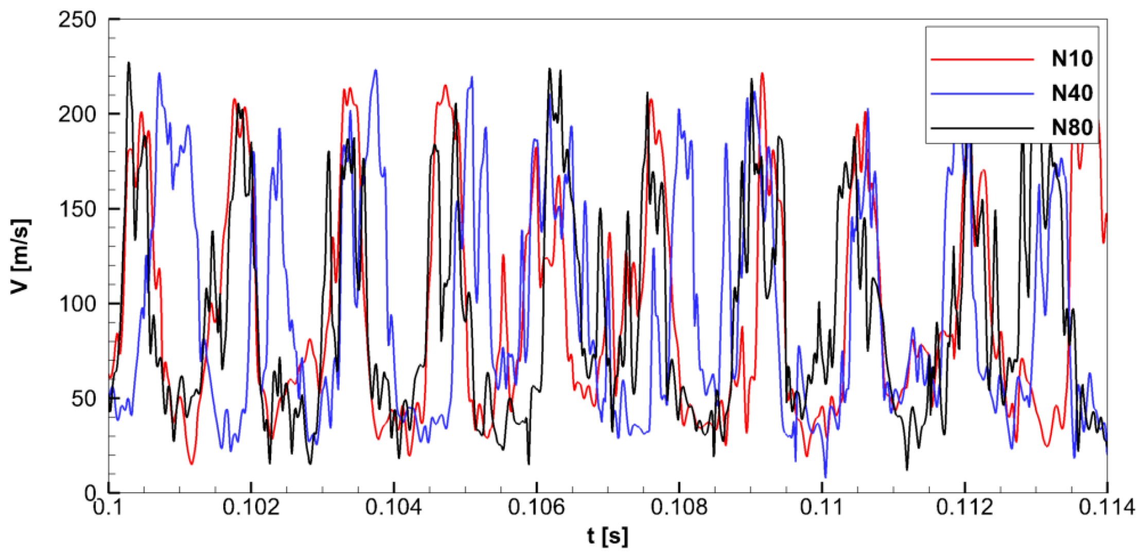
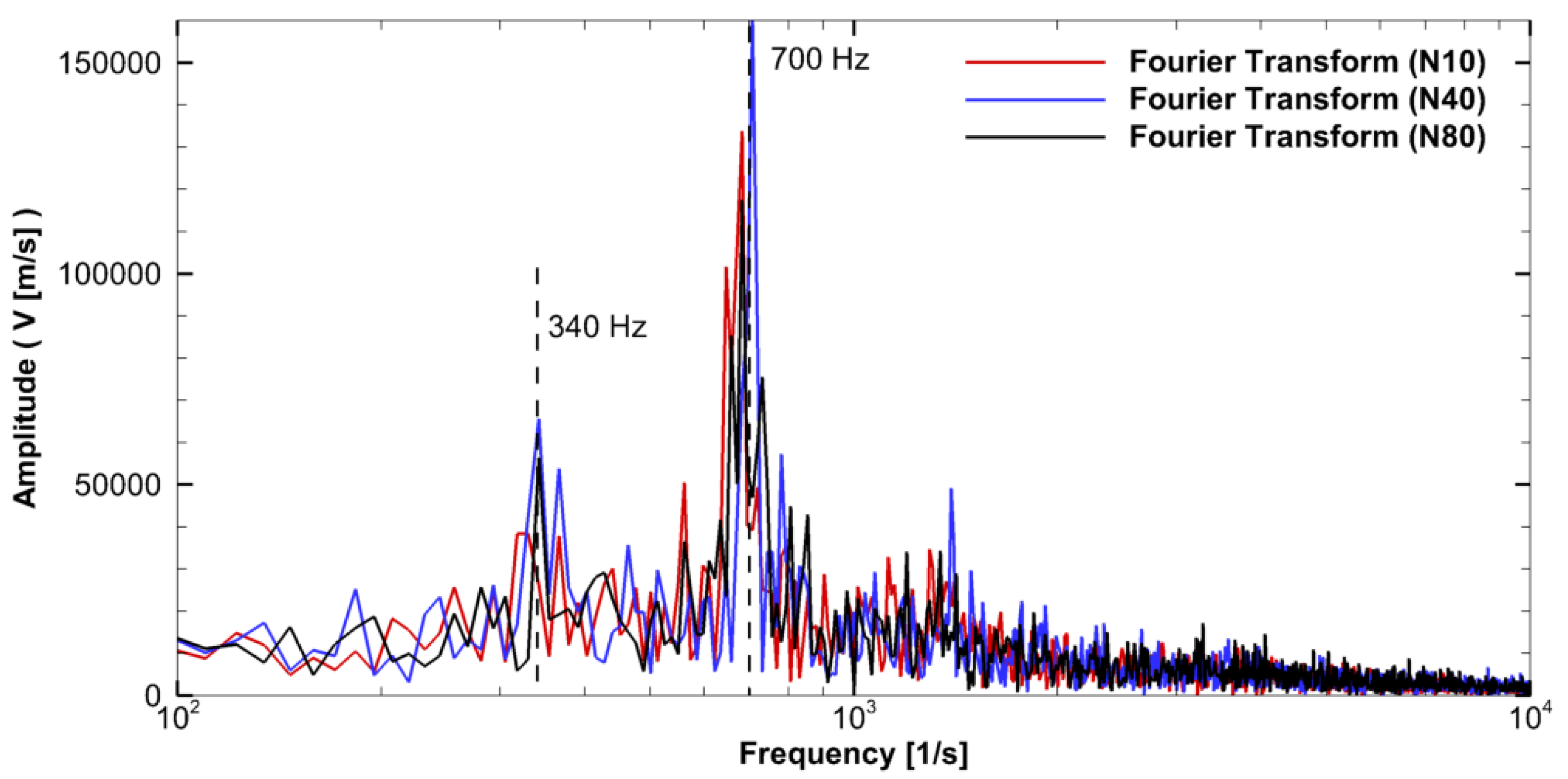
To evaluate the effect of mesh resolution on the time-accurate solutions and jet oscillation frequency, a time history of velocity magnitude is recorded at the downstream of the SWJ actuator exit. The time history of velocity at (6 mm, 0, 0) for 0.006 s (600 data points) are shown in Figure 7 for the coarse, fine, and finest meshes. As a qualitative comparison, the figure shows that the maximum and minimum velocities are similar. However, there is a slight frequency difference between the duration of peak velocities. For a quantitative comparison, a fast Fourier transform (FFT) analysis is performed on the velocity data to identify the jet oscillation frequency using 8192 data points (0.08 s), as shown in Figure 8 and oscillations frequencies are listed in Table 3. In the figure, amplitudes are not scaled. Scaling can be done by dividing the amplitude by the data size of 8192. Moreover, 340 Hz and 700 Hz are marked for easy comparison. The peaks showing jet oscillation frequency appeared near 340 Hz, and higher frequency subharmonic is visible in the spectrum. It is found that the jet oscillates at 341.8 Hz when the finest mesh (N80) is used in the simulation. The deviation from the oscillation frequency is 3.6% and 7.1% for N10 and N20 meshes. In a two-dimensional simulation for the same SWJ actuator and flow conditions, the jet oscillation frequency was reported as 346 Hz [9]. The fine mesh (N40) simulation predicted the same oscillation frequency as the finest mesh. As a result of this section, it was found that the fine mesh (N40) generates similar results as the finest mesh (N80), and therefore, it will be employed for the rest of this study.
3.2. Effect of Mass Flow Rate
The sweeping jet (SWJ) actuator produces a spanwise oscillating jet. The actuator does not have any moving parts, and the oscillating jet is created by the internal geometric structures, including feedback channels, Coanda surfaces, and a mixing chamber [54]. The SWJ actuator has the advantage of having no moving parts from the operational and manufacturing points of view. On the other hand, the fixed actuator is limited to a single operating jet oscillation frequency for a given air supply. Sweeping jet frequency and oscillation angle depend on the geometry of the SWJ actuator and mass flow rate entering through the inlet. Therefore, understanding the effects of the mass flow rate is critical for the development of advanced actuators. To shed some light on the complex flow physics of the SWJ actuator, time-accurate flow simulations are performed for various mass flow rates, as listed in Table 1. The numerical model described in Section 2 is used for the simulations. Time accurate calculations are performed for 0.10 s (10,000 time-steps with a time step size of Δt = 1 × 10⁻⁵ s) for initial transients convect away from the computational domain, and the jet establishes bi-stable oscillating motion. Subsequently, time accurate simulations run for another 0.10 s (34 periods of jet oscillation for g/s) to generate a database from which statistically converged flow quantities analyzed.
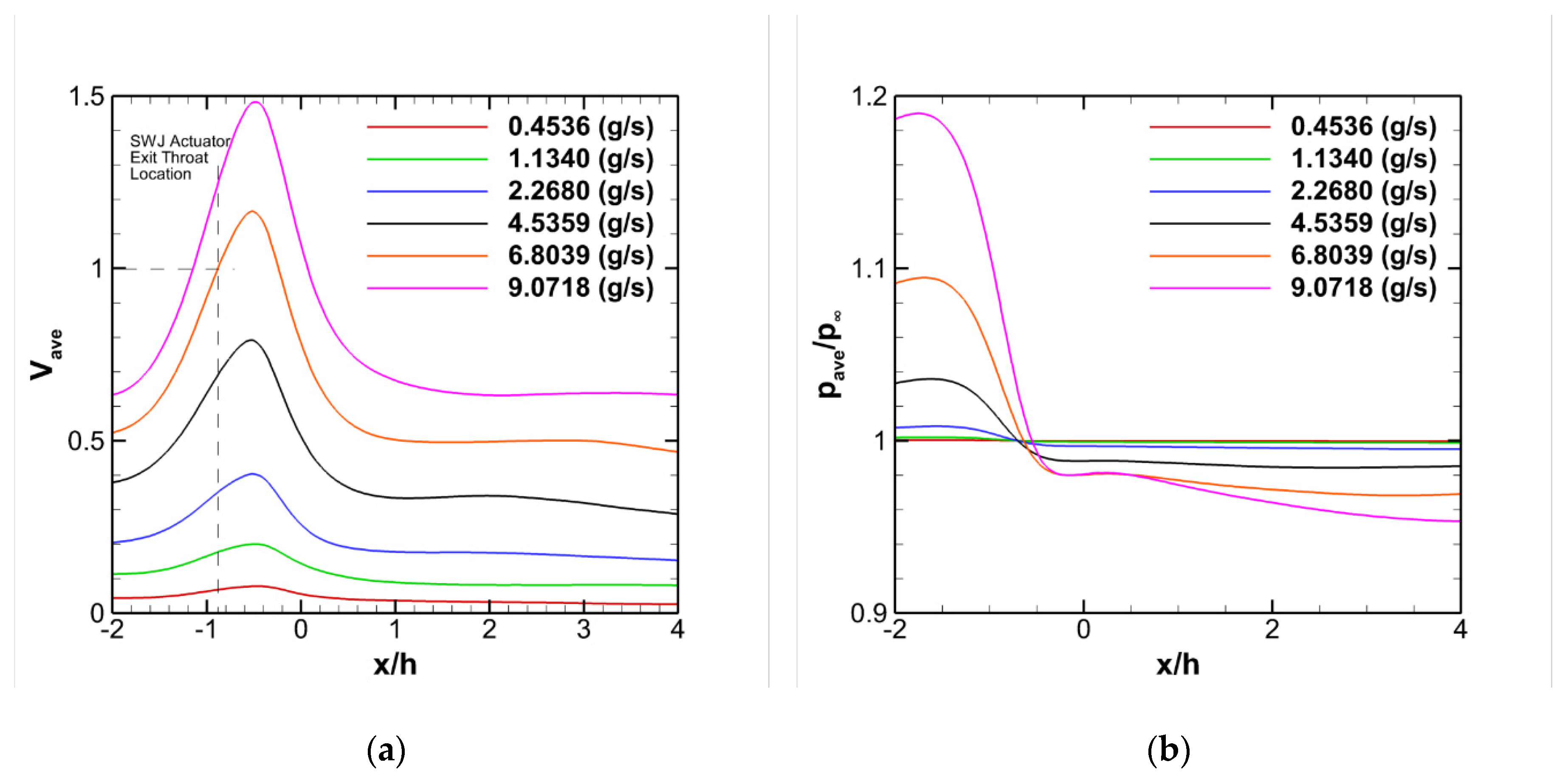
Figure 9 shows the time-averaged velocity magnitude and static pressure along the SWJ actuator symmetry axis (x-axis) for varying mass flow rates. In the time-averaged velocity field, the maximum velocity happens downstream of the exit nozzle throat because of the oscillatory motion of the jet. In the figure, the location of the throat is marked with a gray dashed line. When the actuator pressurized with a mass flow rate of 6.8039 (g/s), the averaged jet speed at exit throat reaches 148.03 m/s, which is also used to non-dimensionalize the velocity profiles in Figure 3a. In this case, the maximum jet flow speed is observed as 172.66 m/s at the downstream of the exit nozzle throat. For all cases, the decay of the velocity magnitude exhibits a similar trend along the x-axis. On the other hand, the time-averaged static pressure sharply decreases in the diverging section of the exit nozzle. It reaches a plateau at the downstream of the actuator, as shown in Figure 9b.
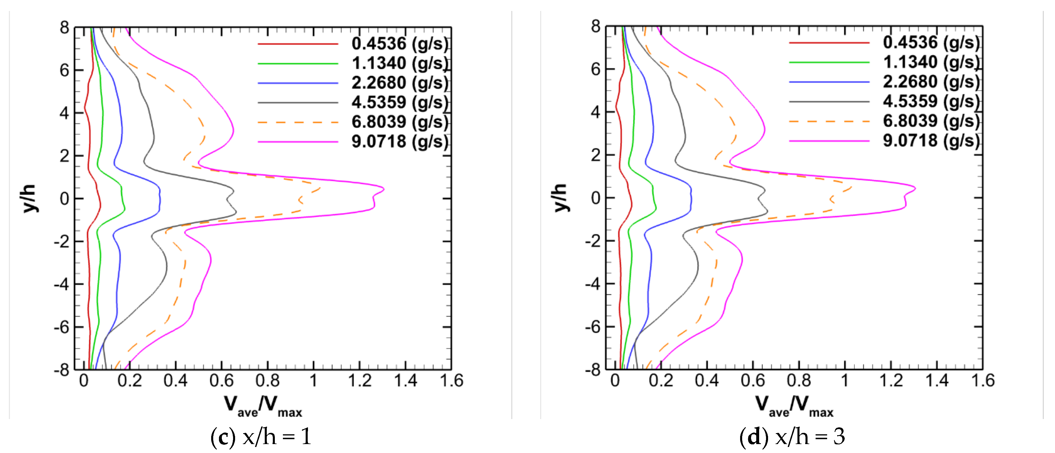
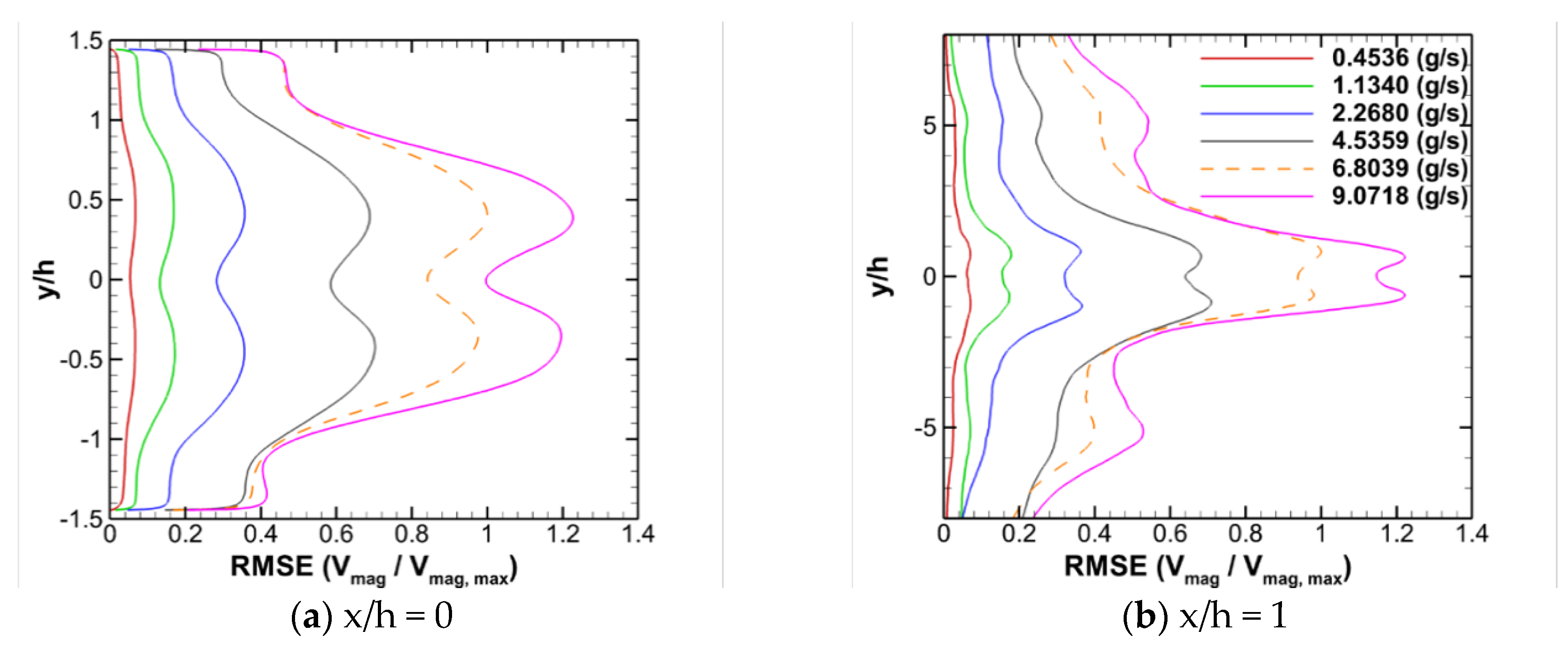
Figure 10 depicts the comparison of time-averaged velocity profiles for several mass flow rates at the SWJ actuator exit nozzle throat and various downstream locations. In the figure, the velocities are non-dimensionalized by the throat velocity of 148.03 m/s for the mass flow rate of 6.8039 g/s. A double peak in velocity profile becomes visible in Figure 10c (x/h = 1) for mass flow rates are greater than 4.5359 g/s where the peak velocity is 40% less than the mass flow rate of 6.8339 g/s. Although peak velocities increase with mass flow rate, the high-speed jet width does not seem to be affected and remains constant for x/h = 1 and 3 stations. Figure 11 shows the root mean square error (RMSE) velocity profiles at x/h = 0 and 1. The RMSE plots show the double peak of the velocity profiles for all mass flow rates indicating the oscillatory behavior of the jet. Moreover, the velocity profile peaks are not located above and below the centerline, which reveals that the oscillating jet spends more time than the centerline.
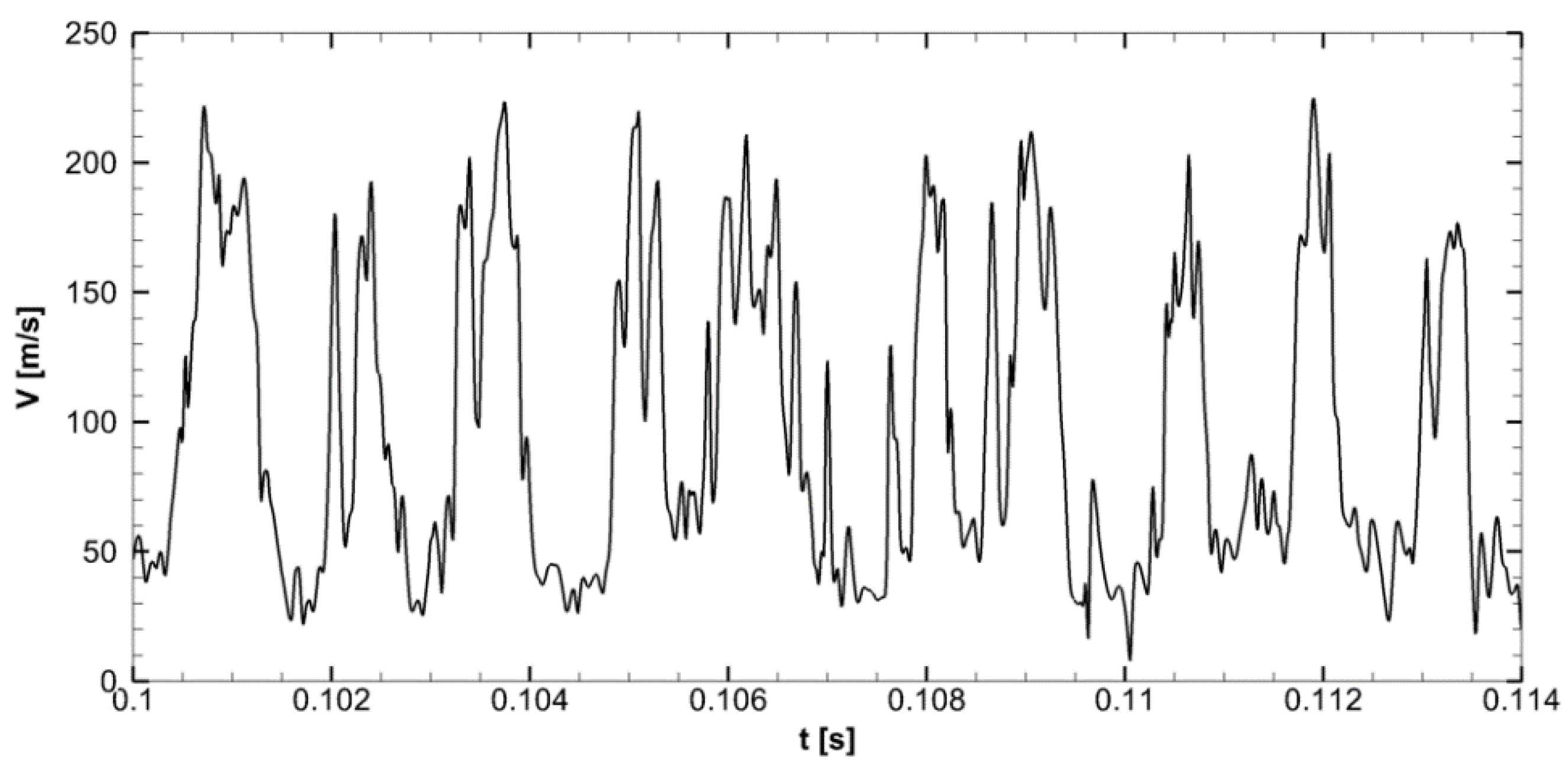
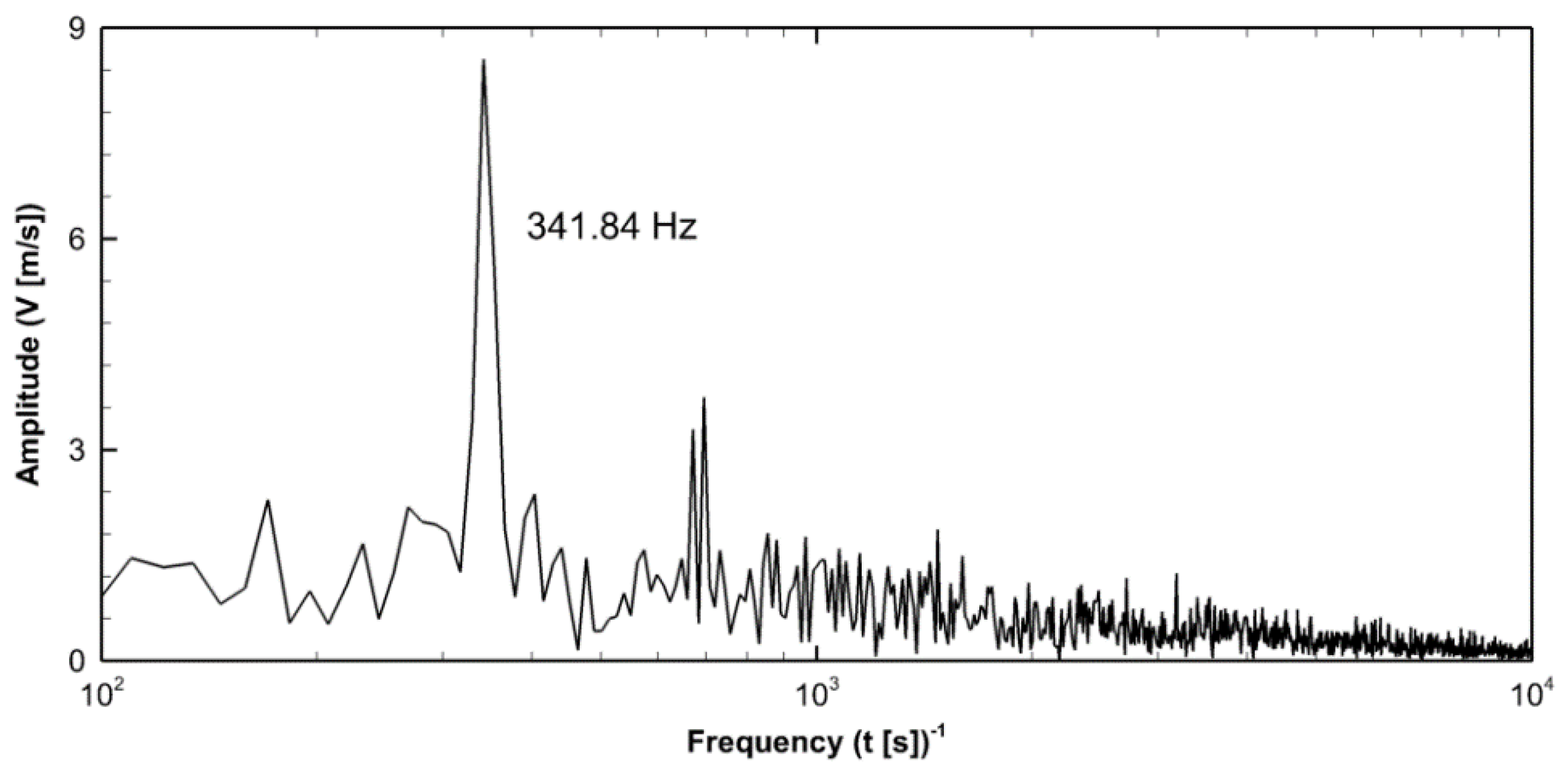
To calculate the jet oscillation frequency, time histories of velocity magnitude are sampled at point (6mm, −10, 0) for the initial conditions given in Table 1. Figure 12 shows the time history of velocity for the mass flow rate of 6.8039 g/s. The plot presents a time history of five periods in 14 ms. High- and low-speed regions are indicating a jet-on and -off behavior of the oscillation jet at the sampling point. Figure 13 shows the result of FFT analysis for velocity data presented in Figure 12. The FFT calculations are performed using the Tecplot [55], and 8192 samples are used. It shows the peak jet oscillation frequency and high-frequency subharmonics. The calculation results are compared with experimental and numerical data of Vatsa et al. [53] in Figure 14, and good agreement is found. In the figure, the Mach number is defined as where is the time-averaged velocity magnitude at the SWJ actuator exit nozzle, is the ratio of specific heats for air , is the gas constant for air , and is the time-averaged static temperature at the same location. The jet oscillation frequency increases with the mass flow rate due to increase in velocities in the mixing chamber and feedback channels. The relationship between jet oscillation frequency and Mach number is modeled using a linear regression line of where R² = 0.97.
Modeling of the turbulence is critically essential for the SWJ actuator simulations. In our current study, we employed the SST k-ω turbulence model. On the other hand, the LBS study employed a hybrid turbulence model where small scales are modeled using a modified k-ε turbulence model, and larger scales are directly resolved [53]. However, Figure 14 shows that both 3D-URANS and 3D lattice Boltzmann simulation (LBS) estimated higher frequencies compared to experimental measurements. Therefore, one can conclude that the two-equation turbulence models cannot capture the complex flow inside and outside of the SWJ actuator, and high-fidelity turbulence modeling such as large eddy simulation (LES) is needed to simulate the SWJ actuator flow, especially when compressibility effects become apparent.
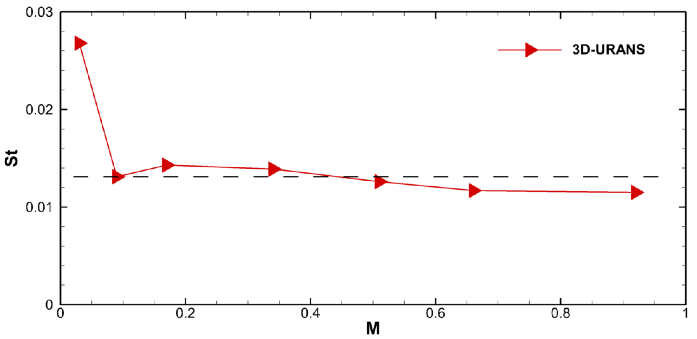
Figure 15 shows the Strouhal number of jet oscillation at various Mach numbers. The Strouhal number is defined as where is the exit nozzle height, is the jet oscillation frequency and is the time-averaged velocity at the exit nozzle throat. It is almost constant with Mach number, and the average is for the present 3D-URANS analysis. In a recent study, Slupski et al. [56] observed a similar behavior of Strouhal number and reported . Their study mostly focused on the incompressible flow range using 2D-URANS simulations and experiments.
4. Conclusions
In this study, the time-accurate flow field of a sweeping jet (SWJ) actuator is numerically investigated using three-dimensional unsteady Reynolds-averaged Navier–Stokes (3D-URANS) model with Ansys Fluent v17.1. Time accurate 3D-URANS simulations are performed for a practical range of mass flow rates providing flow conditions ranging from subsonic incompressible to compressible flows. The actuator geometry is represented using an automated unstructured mesh with two million control volumes. Unstructured hexagonal mesh elements are used to describe intricate geometric details for accurate simulation of fully turbulent compressible flows. The jet oscillation frequency is predicted for all of the operating conditions, and a linear relationship between the jet oscillation frequency and time-averaged exit nozzle Mach number is found (, R² = 0.97). The results from our numerical model were compared with the experimental and numerical data available in the literature, and a good agreement was found. Also, we confirmed that the Strouhal number is almost constant with the Mach number for the subsonic oscillating jet and has an average value of 0.0131. The slight discrepancy in the reported frequency and Strouhal number results are partly attributed to the fidelity of simulations. However, the computational cost of the high-fidelity approaches, such as direct numerical simulations (DNS) or large-eddy simulations (LES) are prohibitive to perform geometric parameter optimization or flow separation control studies. The three-dimensional unsteady Reynolds-averaged Navier–Stokes (3D URANS) model that we presented here provides a computationally inexpensive yet accurate alternative to the researchers.
In the future, geometric parameter optimization, flow separation control, and high-fidelity flow simulations will be performed. The effect of compressibility will also be addressed in subsonic and supersonic flow regimes.
Supplementary Materials
The following are available online at https://www.mdpi.com/2311-5521/5/2/72/s1, Figure S1: Sketch of the Sweeping Jet Actuator, File S1: SolidWorks model of the Sweeping Jet Actuator.
Author Contributions
Conceptualization, K.K.; Formal analysis, F.O. and K.K.; Investigation, F.O. and K.K.; Methodology, K.K.; Supervision, K.K.; Validation, K.K.; Writing—original draft, F.O. and K.K.; Writing—review & editing, F.O. and K.K. All authors have read and agreed to the published version of the manuscript.
Acknowledgments
This work of the authors is supported partially by Oklahoma State University CEAT Start-up and Khalifa University KURIF L1 program.
Conflicts of Interest
The authors declare no conflict of interest.
References
- Anders, S.G.; Sellers, W.L.; Washburn, A.E. Active flow control activities at NASA langley. In Proceedings of the 2nd AIAA Flow Control Conference, Portland, OR, USA, 28 June–1 July 2004. [Google Scholar]
- Whalen, E.A.; Spoor, M.; Vijgen, P.M.; Tran, J.; Shmilovich, A.; Lin, J.C.; Andino, M. Full-scale Flight Demonstration of an Active Flow Control Enhanced Vertical Tail. In Proceedings of the 8th AIAA Flow Control Conference, Washington, DC, USA, 13–17 June 2016; American Institute of Aeronautics and Astronautics: Reston, VA, USA, 2016. [Google Scholar]
- Lin, J.C.; Andino, M.Y.; Alexander, M.G.; Whalen, E.A.; Spoor, M.A.; Tran, J.T.; Wygnanski, I.J. An overview of active flow control enhanced vertical tail technology development. In Proceedings of the 54th AIAA Aerospace Sciences Meeting, San Diego, CA, USA, 4–8 January 2016; American Institute of Aeronautics and Astronautics Inc, AIAA: Reston, VA, USA, 2016. [Google Scholar]
- Stouffer, R.D. Liquid Oscillator Device. U.S. Patent 4508267, 2 April 1985. [Google Scholar]
- Beale, R.B.; Lawler, M.T. Development of a Wall-Attachment Fluidic Oscillator Applied To Volume Flow Metering. In Flow: Its Measurement and Control in Science and Industry; Instrument Society of America: Pittsburgh, PA, USA, 1974; Volume 1, pp. 989–996. [Google Scholar]
- Wang, H.; Beck, S.B.M.; Priestman, G.H.; Boucher, R.F. Fluidic pressure pulse transmitting flowmeter. Chem. Eng. Res. Des. 1997, 75, 381–391. [Google Scholar] [CrossRef]
- Lucas, N.; Taubert, L.; Woszidlo, R.; Wygnanski, I.; McVeigh, M.A. Discrete sweeping jets as tools for separation control. In Proceedings of the 4th AIAA Flow Control Conference, Seattle, WA, USA, 23–26 June 2008; Fluid Dynamics and Co-located Conferences; AIAA Paper 2008-3868. American Institute of Aeronautics and Astronautics: Reston, VA, USA, 2008. ISBN 9781563479427. [Google Scholar]
- Tewes, P.; Taubert, L.; Wygnanski, I. On the use of sweeping jets to augment the lift of a λ-wing. In Proceedings of the 28th AIAA Applied Aerodynamics Conference, Chicago, IL, USA, 28 June–1 July 2010; Fluid Dynamics and Co-located Conferences; AIAA Paper 2010-4689. American Institute of Aeronautics and Astronautics: Reston, VA, USA, 2010; Volume 1, ISBN 9781617389269. [Google Scholar]
- Kara, K. Numerical simulation of a sweeping jet actuator. In Proceedings of the 34th AIAA Applied Aerodynamics Conference, Washington, DC, USA, 13–17 June 2016; American Institute of Aeronautics and Astronautics: Reston, VA, USA, 2016; p. 3261. [Google Scholar]
- Slupski, B.J.; Kara, K. Effects of geometric parameters on performance of sweeping jet actuator. In Proceedings of the 34th AIAA Applied Aerodynamics Conference, Washington, DC, USA, 13–17 June 2016; American Institute of Aeronautics and Astronautics: Reston, VA, USA, 2016. [Google Scholar]
- Duda, B.; Wessels, M.; Fares, E.; Vatsa, V. Unsteady flow simulation of a sweeping jet actuator using a Lattice-Boltzmann method. In Proceedings of the 54th AIAA Aerospace Sciences Meeting, San Diego, CA, USA, 4–8 January 2016; American Institute of Aeronautics and Astronautics: Reston, VA, USA, 2016; p. 1818. [Google Scholar]
- Melton, L.T.P.; Koklu, M.; Andino, M.; Lin, J.C.; Edelman, L. Sweeping jet optimization studies. In Proceedings of the 8th AIAA Flow Control Conference, Washington, DC, USA, 13–17 June 2016; American Institute of Aeronautics and Astronautics: Reston, VA, USA, 2016; p. 4233. [Google Scholar]
- Koklu, M. Effect of a coanda extension on the performance of a sweeping-jet actuator. AIAA J. 2016, 54, 1125–1128. [Google Scholar] [CrossRef]
- Koklu, M.; Owens, L.R. Comparison of sweeping jet actuators with different flow-control techniques for flow-separation control. AIAA J. 2017, 55, 848–860. [Google Scholar] [CrossRef]
- Jurewicz, B.; Kara, K. Effects of Feedback Channels and Coanda Surfaces on the Performance of Sweeping Jet Actuator. In Proceedings of the AIAA SciTech Forum—55th AIAA Aerospace Sciences Meeting, Grapevine, TX, USA, 9–13 January 2017; American Institute of Aeronautics and Astronautics: Reston, VA, USA, 2017. [Google Scholar]
- Aram, S.; Lee, Y.T.; Shan, H.; Vargas, A. Computational fluid dynamic analysis of fluidic actuator for active flow control applications. AIAA J. 2018, 56, 111–120. [Google Scholar] [CrossRef]
- Park, T.; Kara, K.; Kim, D. Flow structure and heat transfer of a sweeping jet impinging on a flat wall. Int. J. Heat Mass Transf. 2018, 124, 920–928. [Google Scholar] [CrossRef]
- Meng, Q.; Chen, S.; Li, W.; Wang, S. Numerical investigation of a sweeping jet actuator for active flow control in a compressor cascade. In Proceedings of the ASME Turbo Expo, Oslo, Norway, 11–15 June 2018; Volume 2A. [Google Scholar]
- Woszidlo, R.; Nawroth, H.; Raghu, S.; Wygnanski, I.J. Parametric study of sweeping jet actuators for separation control. In Proceedings of the 5th Flow Control Conference, Chicago, IL, USA, 28 June–1 July 2010. AIAA Paper 2010-4247. [Google Scholar]
- Phillips, E.; Wygnanski, I.J.; Menge, P.M.; Taubert, L. Passive and Active Leading Edge devices on a simple swept back wing. In Proceedings of the AIAA Aviation 2019 Forum, Dallas, TX, USA, 17–21 June 2019; p. 3393. [Google Scholar]
- Aram, S.; Shan, H. Computational analysis of interaction of a sweeping jet with an attached crossflow. AIAA J. 2019, 57, 682–695. [Google Scholar] [CrossRef]
- Jentzsch, M.; Taubert, L.; Wygnanski, I. Using sweeping jets to trim and control a tailless aircraft model. AIAA J. 2019, 57, 2322–2334. [Google Scholar] [CrossRef]
- Wen, X.; Liu, J.; Li, Z.; Zhou, W.; Liu, Y. Flow dynamics of sweeping jet impingement upon a large convex cylinder. Exp. Therm. Fluid Sci. 2019, 107, 1–15. [Google Scholar] [CrossRef]
- Kim, D.J.; Jeong, S.; Park, T.; Kim, D. Impinging sweeping jet and convective heat transfer on curved surfaces. Int. J. Heat Fluid Flow 2019, 79, 108458. [Google Scholar] [CrossRef]
- Sushanth Gowda, B.C.; Vinuth, N.; Poornananda, T.; Dhanush, G.J.; Paramesh, T. Internal flow analysis on sweeping jet actuator. Int. J. Recent Technol. Eng. 2019, 8, 296–304. [Google Scholar]
- Meng, Q.; Du, X.; Chen, S.; Wang, S. Numerical Study of Dual Sweeping Jet Actuators for Corner Separation Control in Compressor Cascade. J. Therm. Sci. 2019, 1–9. [Google Scholar] [CrossRef]
- Chen, S.; Li, W.; Meng, Q.; Zhou, Z.; Wang, S. Effects of a sweeping jet actuator on aerodynamic performance in a linear turbine cascade with tip clearance. Proc. Inst. Mech. Eng. Part G J. Aerosp. Eng. 2019, 233, 4468–4481. [Google Scholar] [CrossRef]
- Wen, X.; Liu, J.; Kim, D.; Liu, Y.; Kim, K.C. Study on three-dimensional flow structures of a sweeping jet using time-resolved stereo particle image velocimetry. Exp. Therm. Fluid Sci. 2020, 110, 109945. [Google Scholar] [CrossRef]
- Woszidlo, R.; Wygnanski, I. Parameters governing separation control with sweeping jet actuators. In Proceedings of the 29th AIAA Applied Aerodynamics Conference 2011, Honolulu, HI, USA, 27–30 June 2011; Fluid Dynamics and Co-located Conferences; AIAA Paper 2011-3172. American Institute of Aeronautics and Astronautics: Reston, VA, USA, 2011. ISBN 9781624101458. [Google Scholar]
- Koklu, M.; Melton, L.P. Sweeping jet actuator in a quiescent environment. In Proceedings of the 43rd Fluid Dynamics Conference, San Diego, CA, USA, 24–27 June 2013. [Google Scholar]
- Seele, R.; Graff, E.; Lin, J.; Wygnanski, I. Performance enhancement of a vertical tail model with sweeping jet actuators. In Proceedings of the 51st AIAA Aerospace Sciences Meeting including the New Horizons Forum and Aerospace Exposition 2013, Grapevine, TX, USA, 7–10 January 2013; AIAA Paper 2013-0411. American Institute of Aeronautics and Astronautics: Reston, VA, USA, 2013. [Google Scholar]
- Gärtlein, S.; Woszidlo, R.; Ostermann, F.; Nayeri, C.N.; Paschereit, C.O. The time-resolved internal and external flow field properties of a fluidic oscillator. In Proceedings of the 52nd Aerospace Sciences Meeting, National Harbor, MD, USA, 13–17 January 2014; American Institute of Aeronautics and Astronautics Inc.: Reston, VA, USA, 2014; pp. 1–15. [Google Scholar]
- Koklu, M.; Owens, L.R. Flow separation control over a ramp using sweeping jet actuators. In Proceedings of the AIAA AVIATION 2014—7th AIAA Flow Control Conference, Atlanta, GA, USA, 16–20 June 2014; AIAA Paper 2014-2367. American Institute of Aeronautics and Astronautics Inc.: Reston, VA, USA, 2014. [Google Scholar]
- Andino, M.Y.; Lin, J.C.; Washburn, A.E.; Whalen, E.A.; Graff, E.C.; Wygnanski, I.J. Flow separation control on a full-scale vertical tail model using sweeping jet actuators. In Proceedings of the 53rd AIAA Aerospace Sciences Meeting, Kissimmee, FL, USA, 5–9 January 2015; p. 785. [Google Scholar]
- Peters, C.J.; Miles, R.B.; Burns, R.A.; Bathel, B.F.; Jones, G.S.; Danehy, P.M. Femtosecond laser tagging characterization of a sweeping jet actuator operating in the compressible regime. In Proceedings of the 32nd AIAA Aerodynamic Measurement Technology and Ground Testing Conference, Washington, DC, USA, 13–17 June 2016; pp. 1–22. [Google Scholar]
- DeSalvo, M.; Whalen, E.; Glezer, A. High-lift enhancement using fluidic actuation. In Proceedings of the 48th AIAA Aerospace Sciences Meeting Including the New Horizons Forum and Aerospace Exposition, Orlando, FL, USA, 4–7 January 2010. [Google Scholar]
- Seele, R.; Tewes, P.; Woszidlo, R.; McVeigh, M.A.; Lucas, N.J.; Wygnanski, I.J. Discrete sweeping jets as tools for improving the performance of the V-22. J. Aircr. 2009, 46, 2098–2106. [Google Scholar] [CrossRef]
- Cerretelli, C.; Wuerz, W.; Gharaibah, E. Unsteady separation control on wind turbine blades using fluidic oscillators. AIAA J. 2010, 48, 1302–1311. [Google Scholar] [CrossRef]
- Seifert, A.; Stalnov, O.; Sperber, D.; Arwatz, G.; Palei, V.; David, S.; Dayan, I.; Fono, I. Large trucks drag reduction using active flow control. In Proceedings of the 46th AIAA Aerospace Sciences Meeting and Exhibit, Reno, NV, USA, 7–10 January 2008; pp. 115–133. [Google Scholar]
- Woszidlo, R.; Stumper, T.; Nayeri, C.N.; Paschereit, C.O. Experimental study on bluff body drag reduction with fluidic oscillators. In Proceedings of the 52nd Aerospace Sciences Meeting, National Harbor, MD, USA, 13–17 January 2014; American Institute of Aeronautics and Astronautics Inc.: Reston, VA, USA, 2014. [Google Scholar]
- Kara, K.; Kim, D.; Morris, P.J. Flow-separation control using sweeping jet actuator. AIAA J. 2018, 56, 4604–4613. [Google Scholar] [CrossRef]
- Seele, R.; Graff, E.; Gharib, M.; Taubert, L.; Lin, J.; Wygnanski, I. Improving rudder effectiveness with sweeping jet actuators. In Proceedings of the 6th AIAA Flow Control Conference, New Orleans, LA, USA, 25–28 June 2012; AIAA Paper 2012-3244. American Institute of Aeronautics and Astronautics Inc.: Reston, VA, USA, 2012. [Google Scholar]
- Koklu, M. Effects of sweeping jet actuator parameters on flow separation control. AIAA J. 2018, 56, 1–11. [Google Scholar] [CrossRef]
- Hirsch, D.; Gharib, M. Schlieren visualization and analysis of sweeping jet actuator dynamics. AIAA J. 2018, 56, 2947–2960. [Google Scholar] [CrossRef]
- Ott, C.; Gallas, Q.; Delva, J.; Lippert, M.; Keirsbulck, L. High frequency characterization of a sweeping jet actuator. Sens. Actuators A Phys. 2019, 291, 39–47. [Google Scholar] [CrossRef] [Green Version]
- Horne, W.C.; Burnside, N.J. Acoustic study of a sweeping jet actuator for active flow control applications. In Proceedings of the 22nd AIAA/CEAS Aeroacoustics Conference, Lyon, France, 30 May–1 June 2016; American Institute of Aeronautics and Astronautics Inc, AIAA: Reston, VA, USA, 2016. [Google Scholar]
- Seo, J.H.; Zhu, C.; Mittal, R. Flow physics and frequency scaling of sweeping jet fluidic oscillators. AIAA J. 2018, 56, 2208–2219. [Google Scholar] [CrossRef]
- Hirsch, C. Numerical Computation of Internal and External Flows; John Wiley & Sons: Chichester, UK, 1990; Volume 2, ISBN 978-8126539239. [Google Scholar]
- Wilcox, D.C. Turbulence Modeling for CFD, 3rd ed.; D C W Industries: La Canada, CA, USA, 2006. [Google Scholar]
- Gatski, T.B.; Bonnet, J.P. Compressibility, Turbulence and High Speed Flow; Elsevier Ltd.: Amsterdam, The Netherlands, 2013; ISBN 9780123970275. [Google Scholar]
- Menter, F.R. Two-equation eddy-viscosity turbulence models for engineering applications. AIAA J. 1994, 32, 1598–1605. [Google Scholar] [CrossRef] [Green Version]
- Ansys® Fluent, Release 17.1, User Guide; ANSYS, Inc.: Canonsburg, PA, USA, 2016.
- Vatsa, V.; Koklu, M.; Wygnanski, I. Numerical Simulation of Fluidic Actuators for Flow Control Applications. In Proceedings of the 6th AIAA Flow Control Conference, New Orleans, LA, USA, 25–28 June 2012; American Institute of Aeronautics and Astronautics: Reston, VA, USA, 2012. [Google Scholar]
- Raghu, S. Fluidic oscillators for flow control. Exp. Fluids 2013, 54, 1455. [Google Scholar] [CrossRef]
- Tecplot 360 EX, 2019 Release 1, User’s Manual; Tecplot, Inc.: Bellevue, WA, USA, 2019.
- Slupski, B.J.; Tajik, A.R.; Parezanović, V.B.; Kara, K. On the impact of geometry scaling and mass flow rate on the frequency of a sweeping jet actuator. FME Trans. 2019, 47, 599–607. [Google Scholar] [CrossRef] [Green Version]
Figure 1.
A schematic of the sweeping jet actuator, (a) computational domain, and (b) boundary conditions. Reproduced with permission from [9].
Figure 1.
A schematic of the sweeping jet actuator, (a) computational domain, and (b) boundary conditions. Reproduced with permission from [9].

Figure 2.
Computational mesh (N40). (a) Computational domain (XY plane) and (b) close-up view of the sweeping jet actuator mesh. Even with the close-up view, the boundary layer mesh (25 layers) seems like a thick black line. Reproduced with permission from [9].
Figure 2.
Computational mesh (N40). (a) Computational domain (XY plane) and (b) close-up view of the sweeping jet actuator mesh. Even with the close-up view, the boundary layer mesh (25 layers) seems like a thick black line. Reproduced with permission from [9].

Figure 3.
Time-averaged velocity magnitude (a) along the SWJ actuator centerline and (b) close-up to the SWJ exit nozzle.
Figure 3.
Time-averaged velocity magnitude (a) along the SWJ actuator centerline and (b) close-up to the SWJ exit nozzle.

Figure 4.
Time-averaged static-to-reference (a) pressure and (b) temperature ratio along the centerline.
Figure 4.
Time-averaged static-to-reference (a) pressure and (b) temperature ratio along the centerline.

Figure 5.
Time averaged velocity magnitude contour on z = 0 plane for (a) N10 Vave,max = 169.4 and (b) N80 Vave,max = 172.7 m/s. Reproduced with permission from [9].
Figure 5.
Time averaged velocity magnitude contour on z = 0 plane for (a) N10 Vave,max = 169.4 and (b) N80 Vave,max = 172.7 m/s. Reproduced with permission from [9].

Figure 6.
Time-averaged velocity magnitude profiles at various x/h locations.


Figure 7.
Time history of velocity magnitude at (6 mm, 0, 0) point for various meshes at = 6.8039 g/s.
Figure 7.
Time history of velocity magnitude at (6 mm, 0, 0) point for various meshes at = 6.8039 g/s.

Figure 8.
FFT analysis of velocity measurements from various computational meshes ( = 6.8039 g/s).

Figure 9.
(a) Time-averaged velocity and (b) time-averaged static-to-reference pressure ratio along the centerline for different mass flow rates. For the mass flow rate of 6.8039 (g/s), the maximum value of averaged velocity magnitude at the throat is 148.03 m/s. The Vave,max occurs downstream of the throat and is equal to 172.66 m/s.

Figure 10.
Comparison of mean velocity profiles at various downstream locations (a) at the SWJ exit nozzle throat, (b) x/h = 0, (c) x/h = 1 and (d) x/h = 3. For mass flow rate of 6.8039 (g/s), the maximum value of averaged velocity magnitude at throat is 148.03 m/s, at x/h = 0 is 115.67 m/s, at x/h = 1 is 79.32 m/s and at x/h = 3 is 74.08 m/s.


Figure 11.
Comparison of RMSE velocity magnitude profiles at (a) x/h = 0 and (b) x/h = 1. The maximum value of RMSE velocity magnitude at x/h = 0 is 102.1 m/s x/h =1 is 84.6 m/s for the mass of flow rate of 6.8039 g/s.
Figure 11.
Comparison of RMSE velocity magnitude profiles at (a) x/h = 0 and (b) x/h = 1. The maximum value of RMSE velocity magnitude at x/h = 0 is 102.1 m/s x/h =1 is 84.6 m/s for the mass of flow rate of 6.8039 g/s.

Figure 12.
Time history of velocity magnitude at (6 mm, −10 mm, 0) for the mass flow rate of 6.8039 g/s.
Figure 12.
Time history of velocity magnitude at (6 mm, −10 mm, 0) for the mass flow rate of 6.8039 g/s.

Figure 13.
FFT analysis results of the time history of velocity magnitude recorded at (6 mm, −10 mm, 0) for the mass flow rate of 6.8039 g/s. Reproduced with permission from [9].
Figure 13.
FFT analysis results of the time history of velocity magnitude recorded at (6 mm, −10 mm, 0) for the mass flow rate of 6.8039 g/s. Reproduced with permission from [9].

Figure 14.
Jet oscillation frequency for increasing Mach number and comparison with results of Vatsa et al. [53].
Figure 14.
Jet oscillation frequency for increasing Mach number and comparison with results of Vatsa et al. [53].

Figure 15.
Strouhal number of the oscillating jet. ().


Table 1.
Inlet boundary conditions.
| (g/s) | (m/s) | ||
|---|---|---|---|
| 0.4536 | 3.7 | 0.01 | 2197 |
| 1.134 | 9.3 | 0.03 | 5491 |
| 2.268 | 18.6 | 0.05 | 10,983 |
| 4.5359 | 37.2 | 0.11 | 21,965 |
| 6.8039 | 55.8 | 0.16 | 32,948 |
| 9.0718 | 74.4 | 0.22 | 43,930 |
| 11.3398 | 93.0 | 0.27 | 54,913 |
Table 2.
Computational mesh parameters.
| Mesh Name | Element Size (mm) | Number of Elements | Mesh Resolution |
|---|---|---|---|
| N10 | 6.3500 × 10⁻¹ | 397,670 | Coarse |
| N20 | 3.1750 × 10⁻¹ | 749,280 | Normal |
| N40 | 1.5875 × 10⁻¹ | 2,023,860 | Fine |
| N80 | 7.9375 × 10⁻² | 6,672,820 | Finest |
Table 3.
Effect of the mesh size on frequency calculations for ( = 6.8039 g/s).
| Mesh | f (Hz.) | Error (%) |
|---|---|---|
| N10 | 329.6 | −3.6 |
| N20 | 366.2 | 7.1 |
| N40 | 341.8 | 0.0 |
| N80 | 341.8 | Assumed true solution |
© 2020 by the authors. Licensee MDPI, Basel, Switzerland. This article is an open access article distributed under the terms and conditions of the Creative Commons Attribution (CC BY) license (http://creativecommons.org/licenses/by/4.0/).
Share and Cite
MDPI and ACS Style
Oz, F.; Kara, K. Jet Oscillation Frequency Characterization of a Sweeping Jet Actuator. Fluids 2020, 5, 72. https://doi.org/10.3390/fluids5020072
AMA Style
Oz F, Kara K. Jet Oscillation Frequency Characterization of a Sweeping Jet Actuator. Fluids. 2020; 5(2):72. https://doi.org/10.3390/fluids5020072
Chicago/Turabian StyleOz, Furkan, and Kursat Kara. 2020. "Jet Oscillation Frequency Characterization of a Sweeping Jet Actuator" Fluids 5, no. 2: 72. https://doi.org/10.3390/fluids5020072