Generation of Vortex Lattices at the Liquid–Gas Interface Using Rotating Surface Waves

Abstract

In this paper, we demonstrate experimentally that by generating two orthogonal standing waves at the liquid surface, one can control the motion of floating microparticles. The mechanism of the vortex generation is somewhat similar to a classical Stokes drift in linear progression waves. By adjusting the relative phase between the waves, it is possible to generate a vortex lattice, seen as a stationary horizontal flow consisting of counter-rotating vortices. Two orthogonal waves which are phase-shifted by $\pi /2$ create locally rotating waves. Such waves induce nested circular drift orbits of the surface fluid particles. Such a configuration allows for the trapping of particles within a cell of the size about half the wavelength of the standing waves. By changing the relative phase, it is possible to either create or to destroy the vortex crystal. This method creates an opportunity to confine surface particles within cells, or to greatly increase mixing of the surface matter over the wave field surface.

1. Introduction

Vortex lattices, or two-dimensional arrays of stable counter-rotating vortices, have recently been discovered in very different physical and biological systems. Some vortex arrays are spontaneously formed due to the hydrodynamic interaction between motile cells, as in the case of sperm cells [1], or the actively moving micro-particles can nematically align due to collisions, such as collectively moving microtubules driven by molecular motors [2]. In bacterial suspensions, vortex lattices can form due to hydrodynamic interactions between micro-organisms guided by the walls of the micro-fluidic channels [3], or the vortex lattice can be formed by introducing periodic obstacles (pillars) within the bacterial suspension [4]. Such highly ordered patterns as vortex lattices possess very different transport properties in comparison with disordered chaotic motion. It has been suggested that the collective motion of active micro-particles may generate complex fluid currents in various biological systems, such as in the stems of the plants [5].

In the above examples, vortex crystals were formed by the dense populations of actively moving micro-particles. However, it has been recently shown that vortex lattices can be generated using two orthogonal standing surface waves on the water’s surface [6]. Such driven vortex lattices are interesting from several perspectives. The generation of flows using waves opens up the prospects of controlling transport of the surface matter, as well as the dispersion of pollutants, and it is interesting from the point of view of converting wave energy into stationary patterned surface flows. Mathematically, the problem of computing flows produced by surface waves remains very challenging, with just a handful of relatively simple wave configurations solved (see, e.g., [7]). However, in recent years, experimental and numerical studies have demonstrated that waves can generate a broad range of flows by various wave fields. Progressing surface waves can move surface particles either in the direction of wave propagation, or towards the wave source in the so-called “ractor beam” regime [8]. Waves generated using various plungers produce complex stationary surface flows which can be used to either confine surface particles, or to fetch them [8]. Another important class of surface flows investigated extensively since 2011 is the wave-driven two-dimensional turbulence (2D) [9,10,11,12,13,14]. Such turbulence is generated at the surface of liquids perturbed by strongly nonlinear Faraday waves. Though Faraday waves are often described as standing parametrically excited waves, at low dissipation they generate turbulence in the horizontal plane, which reproduces many statistical characteristics of the classical Kolmogorov-Kraichnan 2D turbulence. Paradoxically, nonlinear 3D Faraday waves generate 2D turbulence, whose properties, such as the forcing scale and kinetic energy stored in the inertial interval, can be accurately controlled by changing the frequency and the amplitude of the Faraday waves. Moreover, particle dispersion at the surface is a Taylor diffusion whose diffusion coefficient can also be well-controlled [15,16]. The wave-driven turbulence feeds back onto the wave field, leading to a moderate wave disorder, manifested through the spectral broadening of the wave spectra. Turbulence is driven by Faraday waves by first generating horizontal vortices on the surface, which then strongly interact, forming turbulent flow [17].

Here, we analyse another type of wave-driven flows produced by a superposition of two orthogonal standing waves of small amplitude, as described in Ref. [6]. Separately, each of these waves generate no average flow, and only excite oscillations of the surface particles in the vicinity of nodal points (points of constant surface elevation). However, two orthogonal waves produce a variety of flows which can be controlled by changing the relative phase between the waves. We present a detailed analysis of experimental and numerically modelled flows generated by such waves, and will reveal the mechanics of the generation of the surface vortex lattice.

2. Experimental Setup

In Reference [6], two orthogonal standing waves were generated at the water surface in a square container using two planar paddles which were parallel to the walls of the square container. A standing wave was formed after the reflection of the wave off the container wall. Thus, two paddles and two walls of the container formed a square cavity 300 × 300 mm². Since in the experiments reported here, we aimed at testing the scalability of the flow by going to smaller sizes of the unit cells, we tried to avoid wave dissipation which may have affected the homogeneity of the wave field and of the vortex lattice. In this new experiment, two orthogonal stranding waves were generated using two pairs of planar paddles, each driven by its own computer-controlled electrodynamic shaker (TIRA TV51140, TIRA GmbH, Schalkau, Germany). Now, four paddles formed a square cavity 50 × 50 mm². The opposite paddles moved with the same phase. The phase shift $\varphi$ between two orthogonal pairs of paddles was adjustable in the range of 0-$\pi$ via an arbitrary waveform generator (HP 33120 A, Hewlett-Packard, Palo Alto, CA, USA). The paddle accelerations were measured using two accelerometers ($B\&K$ 4507, $B\&K$, Nærum, Denmark) that provided feedback to the controller (VR9500, Vibration Research Corp., Jenison, MI, USA). This setup was used along with the original configuration 2-paddle configuration. The waves were generated in a frequency range between 2 to 30 Hz. The wave frequency f was chosen to match an integer number of wavelengths $\lambda$ within the cavity. The wave amplitude was controlled by changing the acceleration of the paddles in the range from 0.01g to 0.1g, where g was the gravitational acceleration.

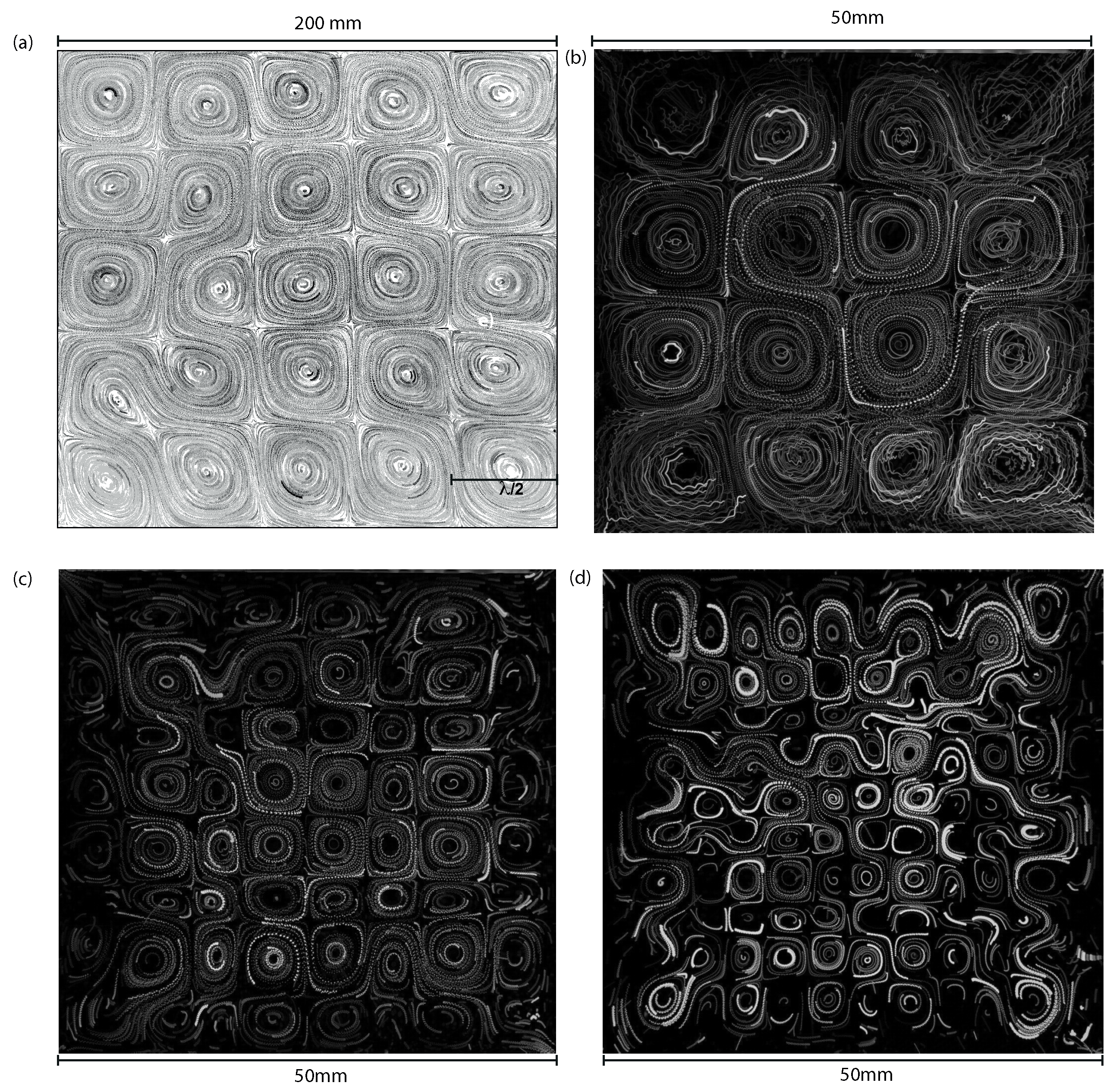
As was demonstrated in [6], when the phase shift between the two orthogonal standing waves approached $\varphi =\pi /2$, the surface flow became ordered and a lattice of vortices was formed. The particle trajectories at $\varphi =\pi /2$ are shown in Figure 1a. A regular pattern of unit cells of the size $L_c=\lambda /2$ was formed, where $\lambda$ is the wavelength of the surface capillary-gravity wave. In adjacent unit cells, the vortices rotated in the opposite (clockwise/anti-clockwise) directions.

Particular attention was paid to boundary conditions at both the oscillating paddles and at the container walls facing them. The presence of a meniscus distorts the wave fields, and affects the spatial control on the phase $\varphi$ in the cavity; it was also recently shown [18] to affect the reflection coefficient of gravity-capillary waves at the wall. To avoid the meniscus at the boundary, we machine grooved in the container walls and paddles such that the contact line was pinned to the wall edge with no meniscus. The wave fields produced in such designed cavities matched the numerically modelled waves well.

In these experiments, the horizontal motion on the fluid surface was visualised by placing 50 μm polyamid particles (specific gravity $SG=1.03$) on the water’s surface. The use of surfactant and plasma treatment of the particles ensured homogenous distribution of the tracer particles. The motion of the suspended particles was captured using a high-resolution fast camera (Andor Neo sCMOS, Oxford Instruments, Abingdon, UK). The velocity fields and particle trajectories were obtained using particle image velocimetry (PIV) and particle tracking velocimetry (PTV).

Diffusive light imaging was used to measure the wave motion. The fluid surface was illuminated using a light-emitting diode panel placed underneath the transparent bottom of the container. A small percentage of milk added to water provides sufficient contrast to obtain a high-resolution reconstruction of the wave field. The absorption coefficient was measured before each experiment, which allows calibration of the surface elevation with a vertical resolution of 80 μm. For 3D PTV measurements, black carbon glass particles which were suspended on the surface were used to simultaneously visualise the fluid particle motion and the waves. Within our experimental parameter range (acceleration and frequency), no difference could be measured between the particle horizontal motion in these experiments and the trajectories of polyamid particles at the surface of water with no milk and surfactant.

The particle trajectories at $\varphi =\pi /2$ for three different frequencies at 9.4 Hz, 16.4 Hz, and 26 Hz are shown in Figure 1b–d. Next, we focus on the mechanism of the flow generation at different phase shifts, from $\varphi =0$ to $\pi /2$.

3. Wave Dynamics

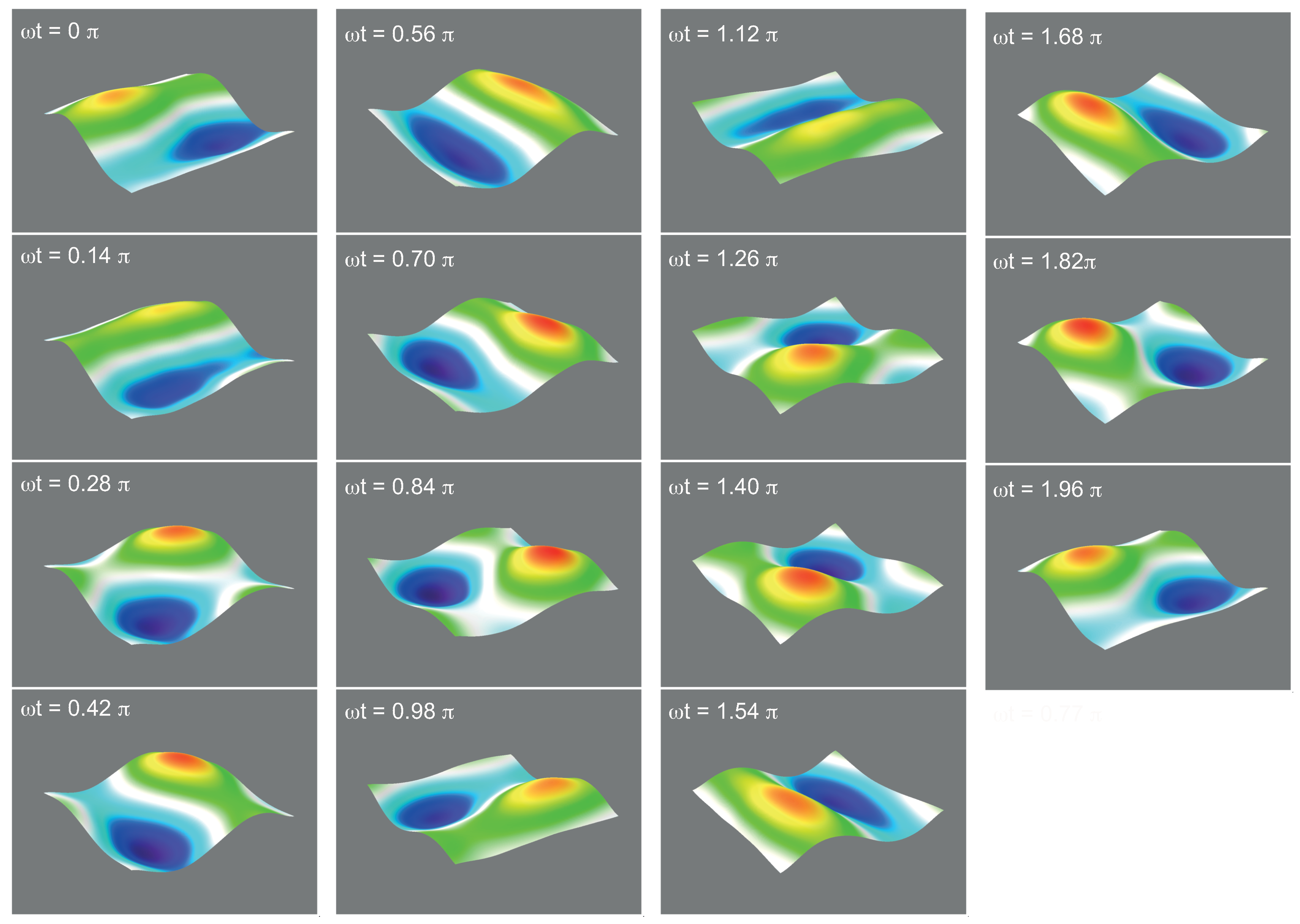
The measured surface elevation produced by two standing waves at the frequency of $f=3.9$ Hz is shown in Figure 2. The field of view shown here is $\lambda \times \lambda$.The phase shift between the two standing waves is $\pi /2$. The wave peak (yellow-red) and trough (blue) rotate around the centre of the cell during one period of the wave. Thus, the two orthogonal waves phase-shifted by $\pi /2$ possess a local angular momentum. This angular momentum originates from the rotation of the wave within the unit cell, as explained below.

The dynamics of the wave can be illustrated using the isolines of the surface elevation. To do this, we used the modelled wave field. The free surface produced by two orthogonal standing waves could be modelled by superimposing two standing waves [19] in the $x,y$ plane:

$$\eta (x,y,t)=2A\left[\cos \right(\omega t\left)\cos \right(Kx)+\cos (\omega t+\varphi \left)\cos \right(Ky\left)\right].$$

(1)

The corresponding velocity potential associated with a Equation (1) is given by:

$$\mathsf{\Phi }(x,y,z,t)=A\cosh \left[K(z+d)\right][\cos \left({\omega }_{1}t\right)\cos \left(Kx\right)+\cos ({\omega }_{2}t+\varphi )\cos \left(Ky\right)],$$

(2)

where K is the wave number, d is the fluid depth, and A is the wave amplitude. The $\mathit{z}$-direction is upwards, with $z=0$ being the level of the undisturbed liquid surface.

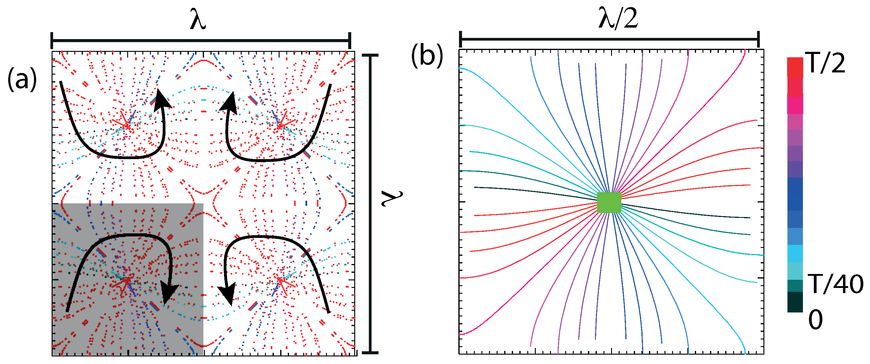
Figure 3a shows the isolines of the wave elevation in the $\lambda \times \lambda$ box. From the $z=0$ isoline shown in (a), it can be seen that the isoline rotates inside the $\lambda /2$ cell. To make it clear, we zoomed into a unit cell of size $L_c=\lambda /2$. The time-varying $z=0$ surface elevation is shown for half a period $T/2$ in Figure 3b. The green square in the middle marks the position of the nodal point where the local amplitude of the standing wave is zero at every instant in time. It can be seen that the isoline rotates continuously at the frequency $\omega$ around the nodal point within the unit cell. During the same time-period, the positions of the peak/trough of the wave traces a square pattern along the edge of the unit cell. This motion of the wave peak defines the edge of the unit cell, seen from the particle trajectories in Figure 1.

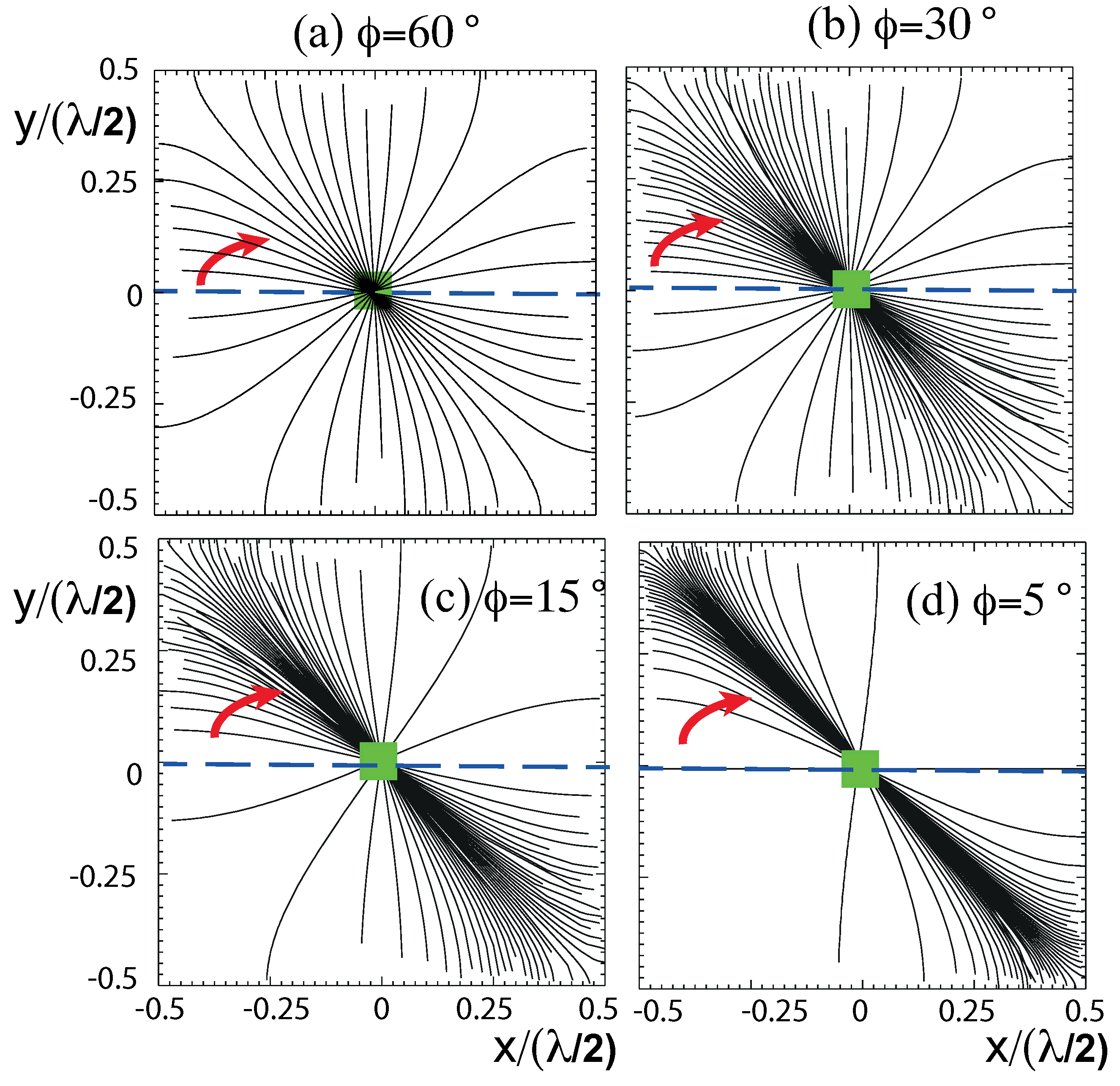
The rotation of the wave peak/trough inside a unit cell can be controlled by changing the phase shift between the two standing waves. This is shown in Figure 4 for four values of the phase shift $\varphi$. The blue dashed line indicates the position of the $z=0$ isoline at $t=0$. The rotation rate of the standing wave decreases with the decreasing phase shift, Figure 4b–d, until it is null when $\varphi =0$. The experimental measurements of the surface elevation are consistent with the model results of Equation (1).

4. Motion of Surface Fluid Particles

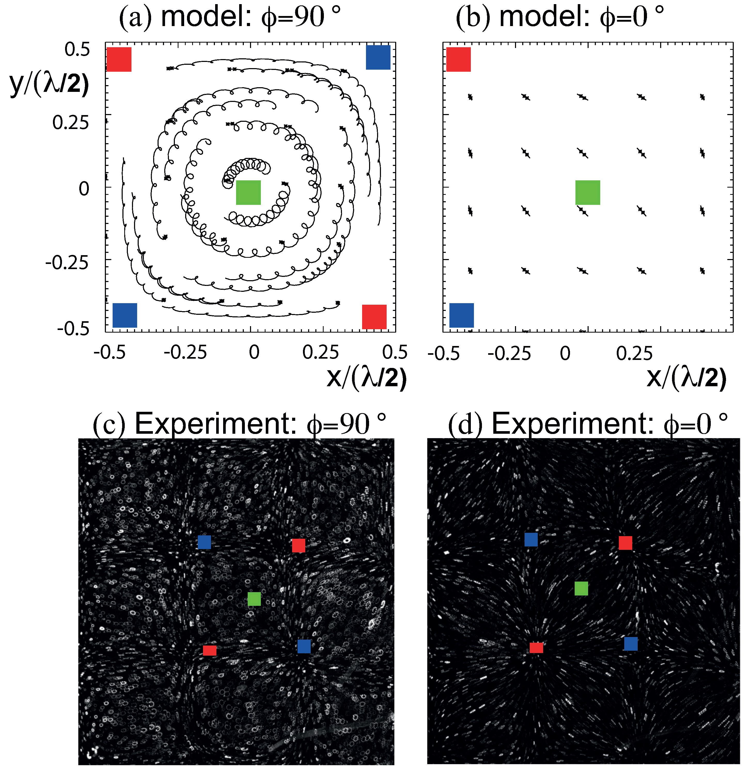
In this section, we analyze particle motion on the water surface perturbed by two orthogonal standing surface waves described above. First, we look at the particle trajectories derived from the numerical integration of the model velocities in the unit cell, Figure 4. The second-order velocities derived from the velocity potential [20,21] were numerically integrated using the fourth-order Runge-Kutta algorithm. The resulting particle trajectories, followed for 10 wave periods, are shown in Figure 5a,b for $\varphi =90°$ and $\varphi =0°$, respectively.

For $\varphi =90°$, trajectories formed nested circles centred around the nodal point of the unit cell, while they also drifted around a nodal point showing trochoidal motion away from the nodes. The particles at the edge of the unit cell traced almost a square, following the motion of the wave peaks and troughs. The drift velocity of the particles $V_D$ decreased toward the centre of the unit cell. For each period of the wave, the particles traced a small circle close to the nodal point. The radius of the gyration $R_g$ decreased from the centre of the unit cell to almost zero at the edge. The particle motion is very different for $\varphi =0°$. Since the wave peaks/troughs trace a straight line at $\varphi =0°$, the particle trajectories are also straight lines forming muscle-shape structures. In the experiments shown in Figure 5c,d, the observed particle trajectories were followed for a short time (one period of the wave). They are very similar to the trajectories generated by the numerical model. Circular trajectories at $\varphi =90°$ and muscle-shaped structures at $\varphi =0°$ could be observed within the unit cells.

However, for long observation times, there were noticeable differences between the experiment and numerical model for the $\varphi =0°$ case. For $\varphi =90°$, Figure 1a, the observed particle trajectories are the same as in the model. In the adjacent unit cells, particles drift in the opposite directions, forming a stable pattern of counter-rotating unit cells. For $\varphi =0°$, at long tracking times, no symmetric stationary patterns are observed. The flow becomes unstable and large-scale structures are formed, partially guided by the container walls. The particle trajectories span over five unit cells as shown in Figure 6a. It is likely that the motion of fluid particles to and away from the peak/trough of the wave (the red isolines shown in Figure 4d becomes unstable, destroying the pattern of oscillating trajectories seen in Figure 5b,d.

5. 3D Reconstruction of the Particle Trajectories

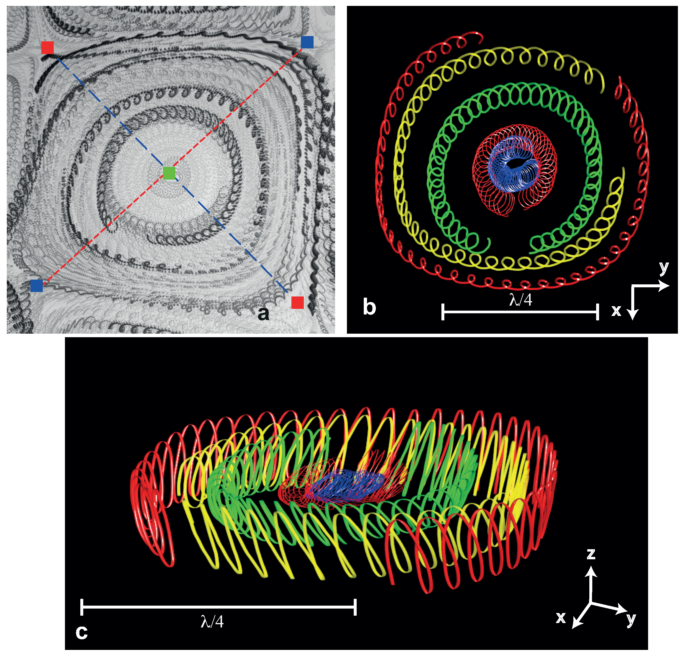
3D Lagrangian trajectories of the surface fluid particles were reconstructed using a combination of a 2D PTV and a diffusive light-imaging technique. The local brightness of the diffused light allows for the detection of the local surface elevation along the trajectory [17]. First, the horizontal motion ($x-y$ coordinates) of a particle was tracked using threshold filters and a nearest-neighbour algorithm. The wave field evolution was then obtained by removing particles from the movies with local filter techniques. Then, the particle elevation (z coordinate) was measured as the wave elevation over a local window (300 μm radius), which was centred on the $x-y$ particle coordinates at a given time. Finally, the 3D trajectories of the particle and the wave field were visualised using the Houdini 3D animation tool (by Side Effects Software).

Rendered 3D trajectories of particles within the unit cell are shown in Figure 7b,c for both the side and the top views. The particles trace a small circle over one wave period; however, the distance traveled during positive half-period is slightly larger than that during the negative half-period. This results in a drift of the orbit in the direction of the wave rotation. This drift occurs along closed loops with a characteristic size $L_c$, much larger than the orbital “circle”. The time-scale of this drift is about 50 wave periods, as seen in Figure 7c. The direction of the orbital drift is opposite in adjacent unit cells and in phase with the rotation of the local wave field.

A model based on the 2D Stokes drift for planar progressive waves [22] was developed to account for the drift observed in a 3D rotating wave field [6]. The incompressible Euler equations were used to model the flow when the surface of an ideal fluid was perturbed by two orthogonal standing waves. For the phase shift between the two waves $\varphi =90°$ the model reproduces trochoid-like trajectories circulating along closed nested orbits within the unit cells in the direction of the rotating wave, which was in agreement with the experiment.

6. Transition to Ordered Vortex Lattice

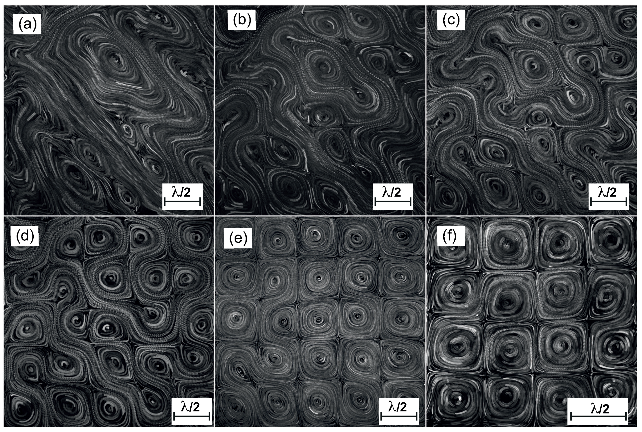
The emergence of the highly ordered pattern was studied by analysing the large-scale particle orbits. In Figure 6a–d, the particle trajectories tracked for 24 wave periods are shown for different phase shifts. For $\varphi =0°$, the flow is disordered. As $\varphi$ increases, the lattice of vortices gradually emerges. The development of the ordered lattice is better observed at lower wave amplitudes, for paddle accelerations of about 0.02g, as shown in Figure 6e.

A similar result can also be observed in liquids with higher viscosity. Experiments were also performed in the glycerol–water solutions with up to 10 times the viscosity of water. Trajectories for waves generated in the glycerol–water solution ($\eta =10$ mPa·s⁻¹) at f = 3.8 Hz, a = 0.03g and $\varphi =90°$ formed a very stable ordered pattern of counter rotating vortices, as seen in Figure 6f.

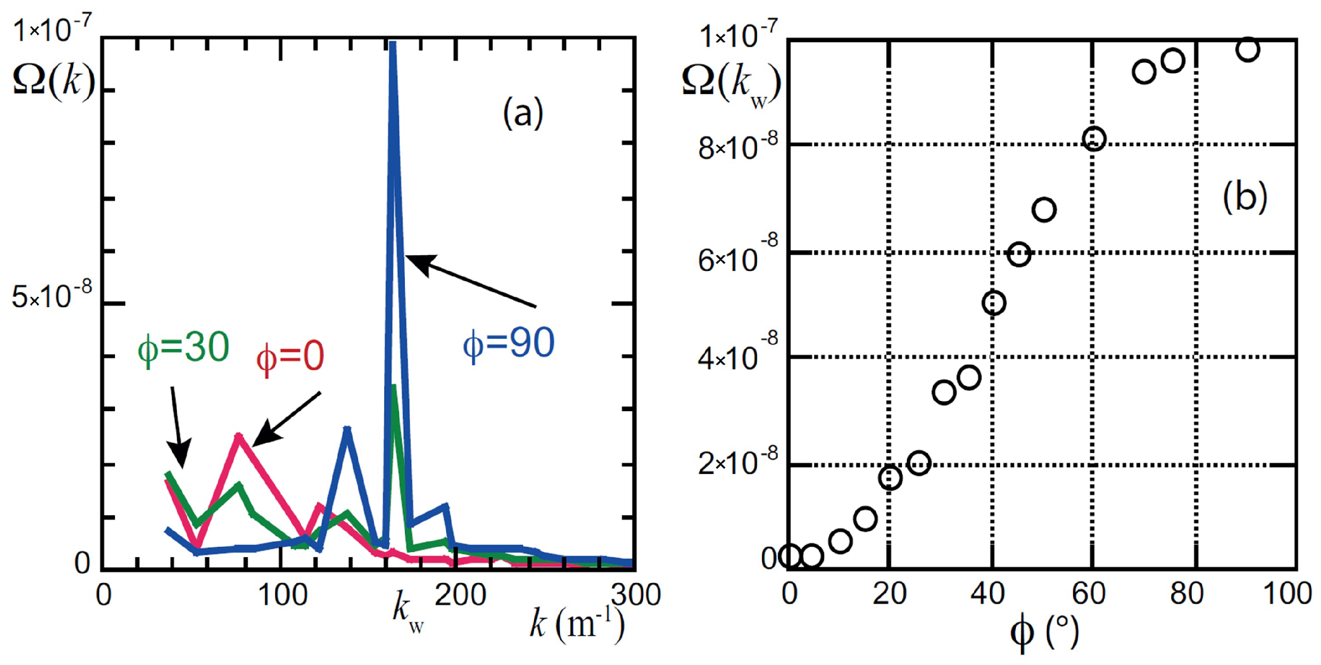
To characterise the development of the vortex lattice quantitatively, we computed the spectrum of the enstrophy $\mathsf{\Omega }={\omega }^2$, or the squared vorticity. Here, the vorticity was $\omega =\frac{\partial v_y}{\partial x}-\frac{\partial v_x}{\partial y}$. Figure 8a shows the Fourier spectra of the enstrophy $\mathsf{\Omega }$ for different relative phases $\varphi$. At $\varphi =0$, the wave-number spectrum spreads over low wave numbers ($k<100$ m⁻¹) corresponding to the large-scale disordered streams seen in Figure 6a. As the phase $\varphi$ increased, the broad distribution at a low wave number was replaced with a strong peak at $k_w=2\pi /L_C\sim 160$ m⁻¹. This peak marks the emerging vortex lattice, with the characteristic spatial scale corresponding to the size of the unit cell. While the phase $\varphi$ is akin to a control parameter of the rotating wave momentum, the magnitude of the peak $\mathsf{\Omega }\left(k\right)$ can be viewed as a structure factor of the vortex lattice. Figure 8b shows that $\mathsf{\Omega }\left(k_w\right)$ grows exponentially in the range $\varphi =[0°,70°]$ by a factor of about 20, and then saturates.

7. Discussion and Conclusions

One of the main advantages of the vortex lattice generation by the rotating waves shown here is its scaleability. Within the parameter range reported here, the unit cell size can be varied by an order of magnitude, while the properties of the periodic patterns remain similar. The generation of the vortex lattices is scalable for surface wave frequencies in the range of 3 Hz up 20 Hz, corresponding to the unit cell sizes from 4 mm to 40 mm.

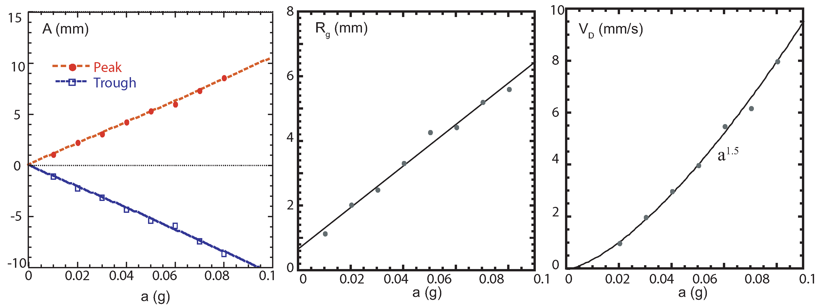
To understand the mechanism of the generation of the vortex lattice, we investigated the relations between the wave height, the radius of the gyro-orbit at the centre of the unit cell (as shown in Figure 5c), and the drift velocity of the fluid particles at the $\varphi =90°$ phase shift, at different accelerations of the paddles. As shown in Figure 9a, the wave amplitude is a linear function of the acceleration. The gyro motion in the centre of the unit cell was most likely due to the gradient of the surface wave elevation. The radius of the gyro-circle changed linearly with the acceleration (wave amplitude), Figure 9b. This is consistent with a linear relation between the gradient of the wave at the node and the wave amplitude. The RMS (root mean square) velocity of the fluid particles changed faster with the wave amplitude, $V_D\sim a^{1.5}$, as seen in Figure 9c. This is indicative of additional nonlinear effects.

It needs to be stressed that the phenomena reported here are different from the vertical circulation (streaming) produced by the standing wave, due to wave attenuation at the boundary or by dissipation, such as those demonstrated in water waves of uniform depth [23] and in acoustic waves [24,25]. In those cases, vertical circulation in cells of $1/4\lambda$ were obtained. In the experiments reported here, a two-dimensional standing wave was generated on a liquid-air interface far away from the boundary ($h/\lambda$ in the range of 0.6 to 2). The unit cells of $1/2\lambda$ were generated on the flow surface.

In summary, we have shown that the drift of fluid particles driven by rotating waves provides a mechanism for the generation of periodic closed particle orbits on the liquid surface. The waves rotated within half-wavelength unit cells. The waves possessed a local angular momentum, which was transferred to the fluid particles. This mechanism produced particle trajectories in the form of a spatially periodic lattice of vortices. At low wave amplitudes, the lattice of vortices interacted only weakly, thus sustaining a stable vortex crystal. In contrast to Faraday waves, whose amplitude and steepness are substantially higher, vortex interactions became strong enough to “melt” the crystal and to generate a developed 2D turbulence. In that case, the vortex lattice can only be observed transiently, as has been previously reported [17]. The presented results prove that the deformation of a liquid–gas interface is a versatile tool for the creation of vertical vorticity in a 2D flow [26,27,28].

An important feature of the flow generated by two orthogonal standing waves is the establishment of unit cells confining nested drift orbits. Such a flow could be used to remotely control diffusion and mixing on the water surface by changing the phase shift between the two standing waves as the control parameter.

References

- Riedel, I.H.; Kruse, K.; Howard, J. A self-organized vortex array of hydrodynamically entrained sperm cells. Science 2005, 309, 300–303. [Google Scholar] [CrossRef] [PubMed]
- Sumino, Y. Large-scale vortex lattice emerging from collectively moving microtubule. Nature 2012, 483, 448–452. [Google Scholar] [CrossRef] [PubMed]
- Wioland, H.; Woodhouse, F.G.; Dunkel, J.; Goldstein, R.E. Ferromagnetic and antiferromagnetic order in bacterial vortex lattices. Nat. Phys. 2016, 12, 341–346. [Google Scholar] [CrossRef] [PubMed]
- Nishiguchi, D.; Aranson, I.S.; Snezhko, A.; Sokolov, A. Engineering bacterial vortex lattice via direct laser lithography. Nat. Commun. 2018, 9, 4486. [Google Scholar] [CrossRef]
- Vicsek, T. Swarming microtubules. Nature 2012, 483, 411–412. [Google Scholar] [CrossRef] [PubMed]
- Francois, N.; Xia, H.; Punzmann, H.; Fontana, F.W.; Shats, M. Wave-based liquid-interface metamaterials. Nat. Commun. 2017, 7, 14325. [Google Scholar] [CrossRef]
- Constantin, A. Nonlinear water waves. Philos. Trans. R. Soc. A 2012, 370, 1501–1504. [Google Scholar] [CrossRef] [PubMed] [Green Version]
- Punzmann, H.; Francois, N.; Xia, H.; Falkovich, G.; Shats, M. Generation and reversal of surface flows by propagating waves. Nat. Phys. 2014, 10, 658–663. [Google Scholar] [CrossRef] [Green Version]
- von Kameke, A.; Huhn, F.; Fernández-García, G.; Muñuzuri, A.P.; Pérez-Muñuzuri, V. Double Cascade Turbulence and Richardson Dispersion in a Horizontal Fluid Flow Induced by Faraday Waves. Phys. Rev. Lett. 2011, 107, 074502. [Google Scholar] [CrossRef] [PubMed]
- Francois, N.; Xia, H.; Punzmann, H.; Shats, M. Inverse energy cascade and emergence of large coherent vortices in turbulence driven by Faraday waves. Phys. Rev. Lett. 2013, 110, 194501. [Google Scholar] [CrossRef] [PubMed]
- Francois, N.; Xia, H.; Punzmann, H.; Shats, M. Wave-particle interaction in the Faraday waves. Eur. Phys. J. E 2015, 38, 106. [Google Scholar] [CrossRef]
- Francois, N.; Xia, H.; Punzmann, H.; Shats, M. Rectification of chaotic fluid motion in two-dimensional turbulence. Phys. Rev. Fluids 2018, 3, 124602. [Google Scholar] [CrossRef]
- Xia, H.; Francois, N.; Punzmann, H.; Shats, M. Tunable diffusion in wave-driven two-dimensional turbulence. J. Fluid Mech. 2019, 865, 811–830. [Google Scholar] [CrossRef]
- Xia, H.; Francois, N.; Faber, B.; Punzmann, H.; Shats, M. Local anisotropy of laboratory two-dimensional turbulence affects pair dispersion. Phys. Fluids 2019, 31, 025111. [Google Scholar] [CrossRef]
- Xia, H.; Francois, N.; Punzmann, H.; Shats, M. Lagrangian scale of particle dispersion in turbulence. Nat. Commun. 2013, 4, 2013. [Google Scholar] [CrossRef] [Green Version]
- Xia, H.; Francois, N.; Punzmann, H.; Shats, M. Taylor particle dispersion during transition to fully developed two-dimensional turbulence. Phys. Rev. Lett. 2014, 112, 104501. [Google Scholar] [CrossRef]
- Francois, N.; Xia, H.; Punzmann, H.; Ramsden, S.; Shats, M. Three-Dimensional Fluid Motion in Faraday Waves: Creation of Vorticity and Generation of Two-Dimensional Turbulence. Phys. Rev. X 2014, 4, 021021. [Google Scholar] [CrossRef]
- Michel, G.; Petrelis, F.; Fauve, S. Acoustic measurement of surface wave damping by a meniscus. Phys. Rev. Lett. 2016, 116, 174301. [Google Scholar] [CrossRef]
- Longuet-Higgins, M.S.; Stewart, R.W. Radiation stresses in water waves; a physical discussion, with applications. Deep-Sea Res. Oceanogr. Abstr. 1964, 11, 529–562. [Google Scholar] [CrossRef]
- Umeki, M. Particle transport by angular momentum on three-dimensional standing surface waves. Phys. Rev. Lett. 1991, 67, 2650–2653. [Google Scholar] [CrossRef]
- Umeki, M. Lagrangian motion of fluid particles induced by three-dimensional standing waves. Phys. Fluids A 1992, 4, 1968–1978. [Google Scholar] [CrossRef]
- Stokes, G.G. On the theory of oscillatory waves. Trans. Cambridge Phil. Soc. 1847, 8, 441–455, Reprinted in: G.G. Stokes (2009). Mathematical and Physical Papers, Volume 1, Cambridge University Press. pp. 197–229. [Google Scholar]
- Longuet-Higgins, M.S. Mass transport in water waves. Philos. Trans. R. Soc. A 1953, 245, 535–581. [Google Scholar] [CrossRef]
- Lord Rayleigh. On the circulation of air observed in Kundt’s tubes and on some allied acoustical problems. Philos. Trans. R. Soc. A 1883, 175, 1–21. [Google Scholar]
- Lighthill, S.J. Acoustic streaming. J. Sound Vib. 1978, 61, 391. [Google Scholar] [CrossRef]
- Saffman, P.G. Vortex Dynamics; Cambridge University Press: Cambridge, UK, 1992. [Google Scholar]
- Feng, Z.C.; Wiggins, S. Fluid particle dynamics and Stokes drift in gravity and capillary waves generated by the Faraday instability. Nonlinear Dyn. 1995, 8, 141–160. [Google Scholar]
- Longuet-Higgins, M.S. Vorticity and curvature at a free surface. J. Fluid Mech. 1998, 356, 149–153. [Google Scholar] [CrossRef]
Figure 1.
Particle trajectories tracked on the water surface at the relative phase shift between two orthogonal standing waves of . (a) 300 mm container, f = 4.58 Hz, water depth h = 80 mm. In the 50 mm container, lattices are generated at (b) f = 9.4 Hz, (c) f = 16.4Hz, and (d) f = 26 Hz. The water depth in the 50 mm container is h=15 mm. The corresponding wavelengths of the standing waves are = 80, 25, 12.5, and 8 mm.
Figure 2.
Experimentally measured temporal evolution of the wave field for two orthogonal standing surface waves, phase-shifted by within a box. Experimental parameters: 300 mm cavity, Hz, mm, mm, video acquisition rate is 55 fps.
Figure 3.
Isolines of the surface elevation at with a phase shift of . (a) within one cell of size . (b) Within a unit cell. The isolines are shown for half a period of the wave . Different colors denote different times.
Figure 4.
Rotation of the isoline of the surface elevation followed over half a wave period . The blue line marks . The red arrow points in the direction of the rotation. (a) , (b) , (c) , and (d) .
Figure 5.
Numerically integrated particle trajectories for (a) , and (b) . The particles were tracked for 10 periods. Experimental particle trajectories for (c) , and (d) . The particles were tracked for one period. Experimental parameters: 300 mm cavity, 3.8 Hz, 0.1.
Figure 6.
Particle trajectories tracked for 24 periods for waves generated at f = 4.58 Hz, = 0.1 at (a) , (b) , (c) , and (d) . (e) Trajectories measured at f = 4.58 Hz, = 0.05 and . Trajectories shown in (a–e) were measured on the surface of water. (f) Trajectories for waves generated in the glycerol–water solution ( mPa·s−1) at f = 3.8 Hz, = 0.08 and .
Figure 7.
(a) Experimentally measured trajectories of particles tracked for ∼40 periods, within a unit cell. The green square in the middle shows the position of the nodal point. The wave peak and trough are shown as red squares, and the blue squares show the position of the saddle points. Reconstructed 3D trajectories shown in the (b) top view (orthogonal projection), and (c) side view (perspective view). Experimental parameters: Hz, = 104 mm, , video acquisition rate is 55 fps.
Figure 8.
(a)Wave number spectrum of the enstrophy for different phase shifts . (b) The onset of the spatially ordered flow is seen as an exponential growth of the peak of the spectrum with an increase in the phase shift in the range of = (0–70)°. Experimental parameters: 30 cm container, 4.58 Hz, 80 mm, 0.1.
Figure 9.
Experimental measurements of (a) the wave peak and trough; (b) the radius of the gyro-circle at the centre of the unit cell; and (c) the drift velocity of the fluid particles at the phase shift of , as a function of the paddle acceleration. Experimental parameters: 300 mm cavity, 3.8 Hz, 0.01g to 0.08g.
© 2019 by the authors. Licensee MDPI, Basel, Switzerland. This article is an open access article distributed under the terms and conditions of the Creative Commons Attribution (CC BY) license (http://creativecommons.org/licenses/by/4.0/).
Share and Cite
MDPI and ACS Style
Xia, H.; Francois, N.; Gorce, J.-B.; Punzmann, H.; Shats, M. Generation of Vortex Lattices at the Liquid–Gas Interface Using Rotating Surface Waves. Fluids 2019, 4, 74. https://doi.org/10.3390/fluids4020074
AMA Style
Xia H, Francois N, Gorce J-B, Punzmann H, Shats M. Generation of Vortex Lattices at the Liquid–Gas Interface Using Rotating Surface Waves. Fluids. 2019; 4(2):74. https://doi.org/10.3390/fluids4020074
Chicago/Turabian StyleXia, Hua, Nicolas Francois, Jean-Baptiste Gorce, Horst Punzmann, and Michael Shats. 2019. "Generation of Vortex Lattices at the Liquid–Gas Interface Using Rotating Surface Waves" Fluids 4, no. 2: 74. https://doi.org/10.3390/fluids4020074