Interaction between a Quasi-Geostrophic Buoyancy Filament and a Heton


1
School of Mathematics and Statistics, University of St Andrews, St Andrews KY16 9AJ, UK
2
Laboratoire d’Océanographie Physique et Spatiale, IUEM, UBO/UBL, 29280 Plouzané, France
*
Author to whom correspondence should be addressed.
Fluids 2017, 2(3), 37; https://doi.org/10.3390/fluids2030037
Submission received: 15 June 2017
/
Revised: 27 June 2017
/
Accepted: 28 June 2017
/
Published: 3 July 2017
(This article belongs to the Collection Geophysical Fluid Dynamics)
Abstract
:We investigate the interaction between a heton and a current generated by a filament of buoyancy anomaly at the surface. Hetons are baroclinic dipoles consisting of a pair of vortices of opposite signs lying at different depths. Such structures have self-induced motion whenever the pair of vortices are offset horizontally. A surface buoyancy filament generates a shear flow since the density perturbation locally modifies the pressure field. The vertical shear induced by the filament offsets the vortices of the heton if vertically aligned initially. Moreover, if the vortex nearer the surface is in adverse horizontal shear with the buoyancy filament, the heton tends to move towards the filament. Conversely, if the upper vortex is in cooperative horizontal shear with the buoyancy filament, the heton moves away from it. The filament is also naturally unstable and eventually breaks into a series of billows as it is perturbed by the heton. Moderate to large intensity surface buoyancy distributions separate the vortices of the heton, limiting its advection as a baroclinic dipole. Instead, the vortices of the heton start to interact strongly with surface billows. Additionally, the vortices of the heton can be partially destroyed by the filament if the shear it induces is sufficiently large.
1. Introduction
Modern satellite imagery and measurements of sea surface temperature and height have provided detailed maps of the complex fluid dynamics occurring at the surface of the oceans. These measurements have also allowed one to infer a limited part of the dynamics in the ocean interior, through the analysis of surface signatures imprinted by subsurface eddies or “vortices” (see e.g., [1,2]). These vortices however do not always provide a discernible, unambiguous surface signature. In general, the role of such vortices is not well understood due difficulties in their detection, yet they may contribute strongly to the flow field as a whole. To make progress, theoretical modelling is needed to study the fundamental interactions occurring between dynamical features at the ocean surface and those at depth, in particular the impact of subsurface vortices.
Vortices are ubiquitous in the oceans (see [3,4,5] for a sample of the vast and ever extending literature). It is also well-established that vortices are key dynamical features in the oceans, contributing a large part of the overall transport of momentum, heat and other tracers such as salinity [6]. Although an isolated vortex does not move, a population of vortices moves as a consequence of their mutual interactions and of their interaction with other dynamical features such as jets and currents. The present paper considers the evolution of a “heton”, or baroclinic dipole, interacting with a surface filament of anomalous buoyancy. Hetons consist of two vortices lying at different depths and were proposed in [7,8,9,10] as an elementary mechanism for heat transport in the oceans. Hetons may form as a result of the baroclinic destabilisation of coastal currents [11] or of deep oceanic jets [12,13]. Other possible formation mechanisms are summarized in [14]. Hetons have been extensively studied in idealized layer models with a small number of layers, and a comprehensive review of the relevant literature can be found in [14]. In this paper we consider continuously stratified, three-dimensional hetons. Such hetons were first studied in detail in [15,16]. These studies confirmed that compact hetons tend to be stable while wide hetons, whose vortices have large radius-to-height aspect ratios, are prone to baroclinic instability. However, this instability can been suppressed for sufficiently large horizontal or vertical offsets between the vortices [16].
Buoyancy filaments are also commonly observed at the sea surface [17,18,19]. The linear stability of such filaments and their nonlinear evolution has been the focus of several studies, see [20,21,22]. Recently, Reinaud et al. (2016) [23] considered the interaction between a surface buoyancy filament and a monopolar vortex located below the filament, in the ocean interior. Typically, the vortex triggers the most unstable mode of deformation of the filament, but intense filaments may shear out the vortex, especially when the vortex is in an adverse (counter-rotating) horizontal shear induced by the filament.
The interaction between vortices and shear flows has been considered in many previous studies. For example, a vortex pair moving within a large-scale two-dimensional deformation flow may in general induce chaotic mixing of passive tracers [24]. A more closely related study is that of Bell (1990) [25] who considered the interaction between a single vortex and a potential vorticity front in a single layer quasi-geostrophic flow. The vortex induces a perturbation to the front which radiates away as Rossby waves, and these waves in turn cause the vortex to move toward or away from the front to conserve linear impulse. The destabilization of a unstable jet by a single vortex has also been studied in [26], for both a two-dimensional barotropic and a single layer shallow water fluid. The flow induced by the vortex destabilizes the jet which subsequently breaks into dipoles. The dipoles may then interact with the vortex. In the present paper, by contrast, we consider a self-propagating vortex, a tilted heton, whose tilt and subsequent propagation are caused by the vertical shear induced by a surface buoyancy filament. The mechanism of vortex motion and the vortex–filament interaction differ substantially from those discussed in previous studies.
We explain below how the vertical shear induced by a surface filament tilts a heton that is initially vertically aligned. This causes the heton to start moving either towards or away from the filament. If the upper vortex of the heton is in adverse shear with the filament, the heton initially moves towards the filament. Conversely, if the upper vortex is in cooperative shear, the heton moves away from the filament. The filament destabilizes and breaks up into billows. Subsequently, the vortices of the heton may interact strongly with the surface billows, especially for moderate to intense filaments. This affects the motion of the heton by further separating the vortices. In extreme cases, the shear induced by the filament can tear the vortices apart.
2. Mathematical Model and Geometry
2.1. Governing Equations
We consider a three-dimensional, rapidly-rotating and strongly-stratified flow. We denote as the Coriolis frequency associated with the background rotation, where is the Earth’s rotation rate and is the latitude. We denote N as the buoyancy frequency associated with the stable stratification, , where g is the gravitational acceleration, is the mean, background density, and is the physical vertical coordinate. For simplicity, we assume both f and N are constant. It is then convenient to define as a stretched vertical coordinate since typically –100 over wide areas of the ocean [27]. In the limit of small Rossby number , where U is a characteristic horizontal velocity, and L is a characteristic horizontal length, and in the limit of small Froude number , where H is a characteristic vertical length, the primitive (non-hydrostatic) equations can be reduced asymptotically to the much simpler quasi-geostrophic (QG) equations, (see e.g., [28]). Typically, these equations are derived assuming that the Burger number , but in fact they are valid over the wider range when .
The QG equations have just one prognostic variable, the potential vorticity , or surface buoyancy at the upper surface. Both are anomalies relative to a uniform background state. Both are advected materially, i.e., transported conservatively, in the absence of diabatic and frictional effects. The advecting flow field is itself determined by linear “inversion” relations (Poisson problems) involving q and b (see below). Moreover, this flow field is layerwise two-dimensional (vertical velocity is negligible) and incompressible. This means that the area enclosed between any two isolevels of q or b cannot change in time.
The equations read as follows. Using the linearity of the inversion relations relating the streamfunction to q and b, the streamfunction is split into two parts,
The part is the streamfunction induced by the potential vorticity q, hereafter “PV”, in the ocean interior, while the part is the streamfunction induced by the surface buoyancy b. The inversion relations are:
where is the Laplacian in the stretched coordinates. Additionally, boundary conditions are required. Here, we take the flow to be horizontally periodic, with period , without loss of generality. In the vertical, we assume the flow is bounded below by an impermeable, flat surface at and above by the ocean surface at . Under the QG approximation, deformations of the free upper surface are negligible, and it is consistent to impose boundary conditions at a flat surface. As the vertical velocity is negligible, the boundary conditions instead come from the hydrostatic approximation, and thus relate the vertical derivative of the streamfunction to the buoyancy. At the bottom, we assume the buoyancy (anomaly) is zero. Hence, the boundary conditions, using hydrostatic balance, are:
Notably, the total streamfunction then satisfies the appropriate boundary conditions. Given , the advecting (geostrophic) horizontal velocity may be calculated from:
The dynamical equations are complete once we add the conservative evolution equations satisfied by the PV and the (scaled) surface buoyancy:
where is the material derivative.
The equations are solved numerically using the contour-advective semi-Lagrangian (CASL) algorithm, developed originally for three-dimensional QG flow simulations by [29], and extended to include variable surface buoyancy by the authors of [30]. The inversion equations are solved on a grid in the interior, and on a grid of resolution at the surface. The resolution is increased at the surface as the surface dynamics are expected to generate fine scales [20,21,22]. The “surgery” scale , introduced in [31], used for regularising the contours (or jumps) representing the Lagrangian PV and buoyancy fields, is set to of the inversion grid length, i.e., . Finally the equations are integrated in time using a fourth-order Runge-Kutta integration scheme, with a time step adapted to resolve the local stretching of the buoyancy contours. Specifically, , where is the contour stretching rate between two adjacent nodes i and on a contour.
2.2. Geometry and Problem Setting
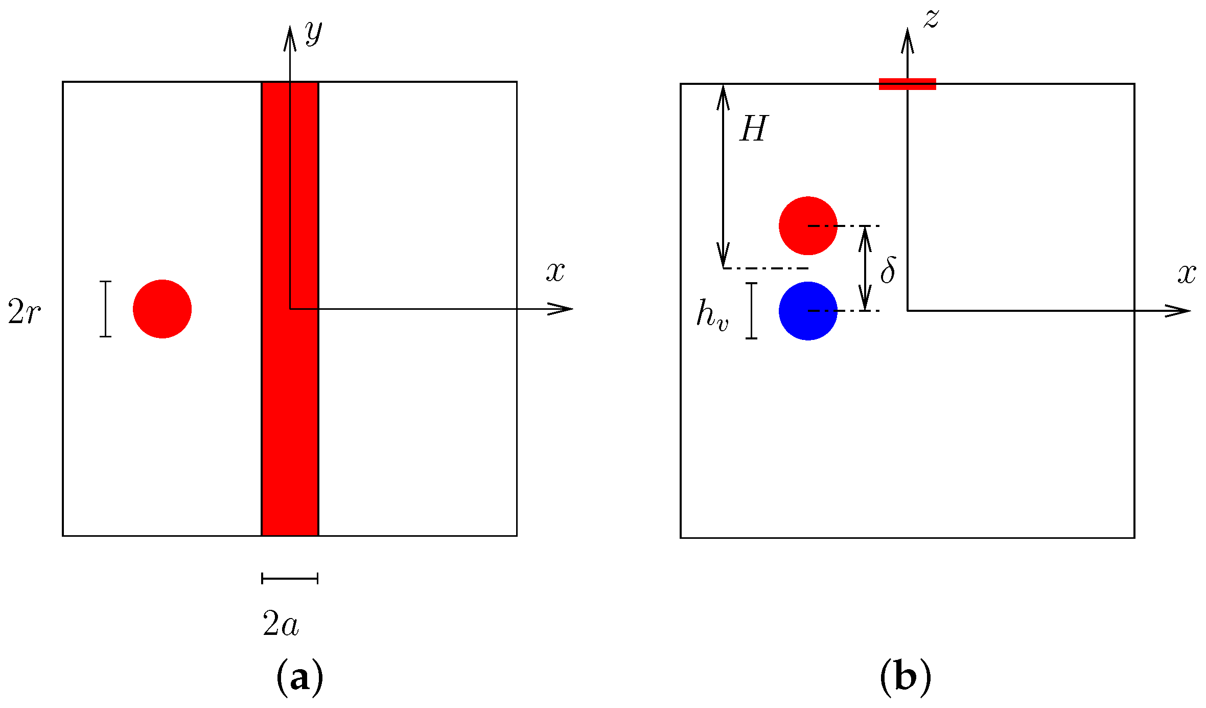
The geometry of the flow is depicted in Figure 1. The computational domain is periodic in x and y, and of depth (in the stretched z coordinate). Initially, a straight buoyancy filament is placed on the surface parallel to the y-axis, between and a. The buoyancy distribution is prescribed by:
This distribution induces a uniform horizontal shear, , at the surface for , (see [23]). Next, a heton is placed in the interior of the computation domain. The heton consists of two equal spheroidal vortices of uniform PV but opposite signs, . Each vortex has a height and a horizontal radius r. Initially, their centres are horizontally aligned and offset in the vertical by a distance . The midpoint between the centres is located at a depth H below the surface. We define as the ratio of the uniform horizontal shear in the buoyancy filament to the PV in the upper vortex—referred to as vortex 1. This dimensionless parameter measures the relative strength of the filament compared to the intensity of the heton. A large value of characterizes the interaction between an intense surface filament with a relatively weak heton, while a small value of characterizes the interaction of a weak filament with a relatively intense heton.
3. Results
3.1. Model of a Steady Filament and a Singular Heton
We first present results obtained from a simplified model of the flow. In this model, the ocean is assumed to have an infinite depth () and the heton is idealized by two singularities—QG point vortices—of strength (the volume-integrated PV divided by ). The surface filament is fixed and thus the induced flow is time-independent. This flow is obtained semi-analytically by performing the inversion exactly in spectral space. Since the surface buoyancy distribution is a function of x only, the streamfunction is a function of x and z only. By taking a Fourier transform of both and in x, we obtain the following inversion problem for each horizontal wavenumber k (denoted by a superscript):
The solution is:
where,
by virtue of the boundary condition at . From this, the velocity field in spectral space is given by:
Finally, the flow field in physical space, , is recovered by an inverse Fourier transform (summing the real part of over all k).
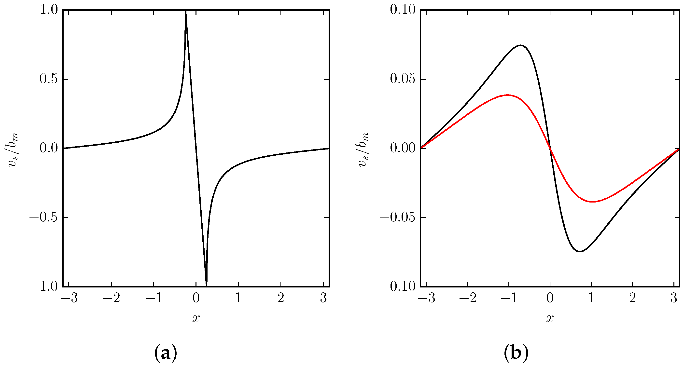
A few cross sections of at constant z are illustrated in Figure 2 for a filament with half-width . The flow at the surface , denoted , is shown in Figure 2a, while the flow at the depths of the upper and lower vortices comprising the heton, denoted and respectively, is shown in Figure 2b (as the black and red curves). We now examine how the heton moves in such a flow field. For purposes of illustration, we assign a strength to vortex 1 and to vortex 2. We place the vortices initially at and . In this aligned configuration at , the self-induced velocity of the heton is zero. Subsequently, the vortices separate in y since the filament induces a velocity in the y direction only, and is greater in magnitude than . The offset of the vortices in y subsequently generates a self-induced motion of the heton in the x direction. By symmetry, the x velocity component is the same for both vortices, so for all time. No self-induced motion is ever generated in the y direction. We conclude that the vortices move in y only due to the presence of the filament, and in x only due to their mutual interaction. This is in contrast with the drift.
Consider a filament with maximum buoyancy . Referring to Figure 2, when , the velocity and decreases with depth, i.e., . The positive vortex 1 is therefore offset to a location . This leads to a self-induced velocity of:
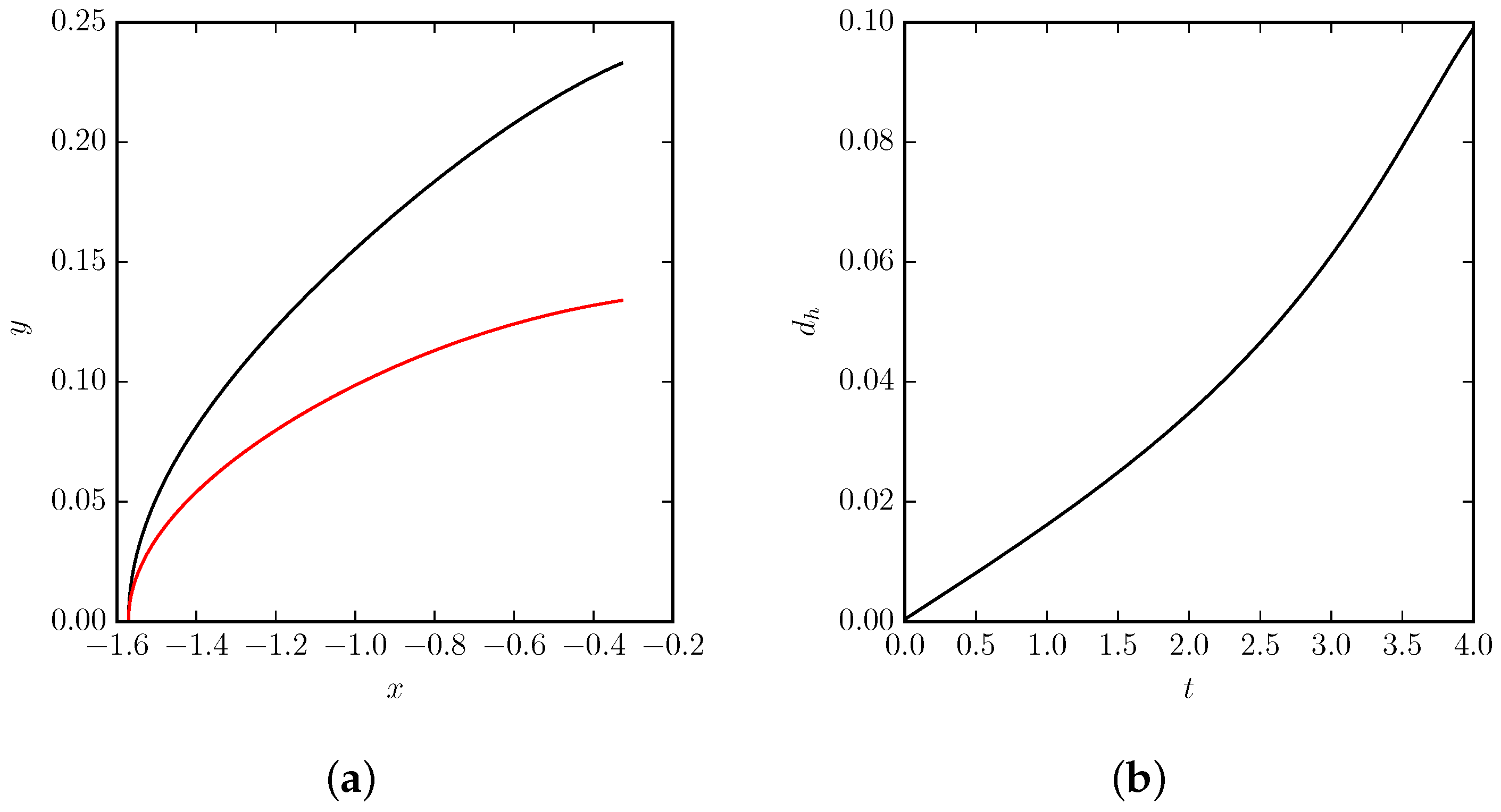
causing the heton to move towards the filament (underneath it). The computed trajectories of the vortices and their horizontal separation versus time t are shown in Figure 3. They confirm that the vortices separate so long as where , and that they continue to move toward increasing x. Once the vortices pass , the vertical shear reverses and the vortex separation decreases. Ultimately, the vortices come to rest at an x position opposite their initial x position, only to separate again and move toward the filament. This continues periodically thereafter. In the opposite situation where vortex 1 has negative strength, i.e., changing to and to 1, the two vortices separate but move away from the filament, ultimately at a constant speed.
A major deficiency of this idealised model is its neglect of the filament dynamics. The vortices will induce perturbations on the filament, and these will generally destabilise the filament. Thus, it is unlikely that the heton will pass under the filament repeatedly. Moreover, finite volume vortices may be expected to behave differently than point vortices. Finite volume vortices are sensitive to both horizontal and vertical shear, and the induced vortex deformations affect their motion. These two effects influence the overall evolution of the flow, as discussed in the following subsections.
3.2. Full Nonlinear Dynamics
We next consider the full nonlinear evolution of a surface buoyancy filament and a finite core heton. Besides the vortex separation effect studied above, now the external velocity field of the heton deforms the surface filament. The buoyancy filament is known to be unstable, see [20,21,22,23,32]. In particular, Reinaud et al. (2016) have shown that the fastest growing mode for a filament having a basic-state buoyancy profile occurs at the dimensionless longitudinal wavenumber with growth rate .
Another new effect is the deformation of the vortices themselves. For a heton moving towards the filament, the vortex nearer the surface must be in adverse horizontal shear with the filament (a shear which slows the rotation of the vortex [33]). Conversely, for a heton moving away from the filament, the vortex nearer the surface must be in cooperative horizontal shear. Previous studies have shown that adverse horizontal shear is significantly more disruptive than cooperative shear [23,34,35]. Hence, a heton which moves towards a surface filament is likely to undergo significant deformation and, in some cases, even partial destruction.
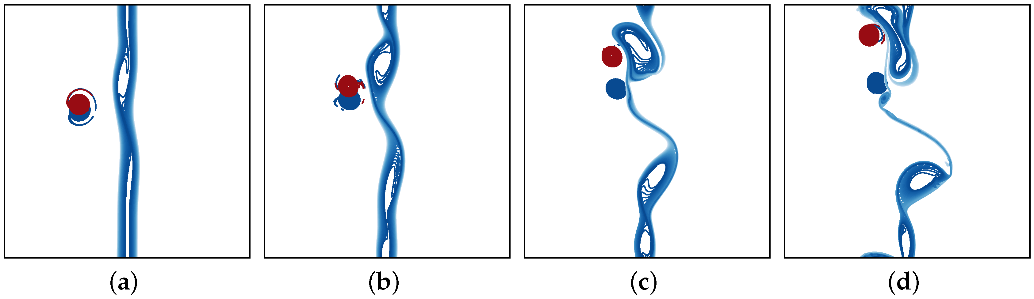
The parameters used for the simulations described below are summarised in Table 1. We start with the reference case 1 which exhibits features common to many cases investigated. Here, the half-width of the filament is set to , and each vortex of the heton is taken to be a sphere (in the stretched coordinates). We take so that , and choose the mean depth of the heton to be . The PV of the vortices is set to . The vortices are initially aligned horizontally with and , while they are displaced vertically by so that and . Vortex 1 is therefore closest to the surface. We choose the vertical offset to be , which means that the two vortices are touching at their mean depth. We set to give a dimensionless shear of . Vortex 1 rotates in the counter-clockwise direction () while vortex 2 rotates in the clockwise direction (). Vortex 1 is therefore in adverse horizontal shear with the surface filament.
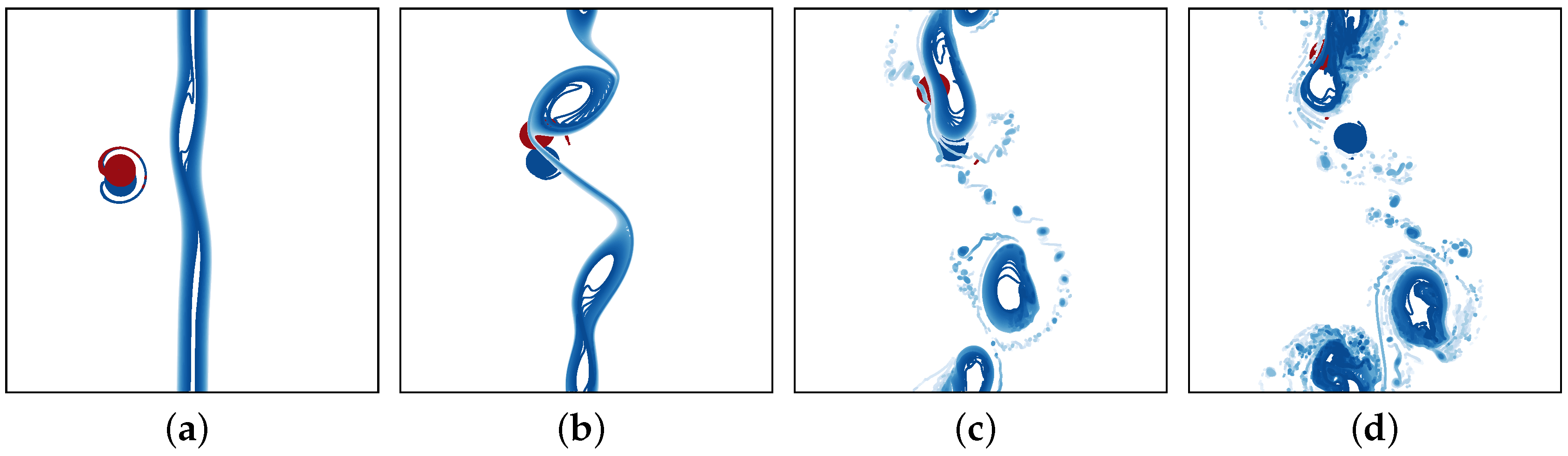
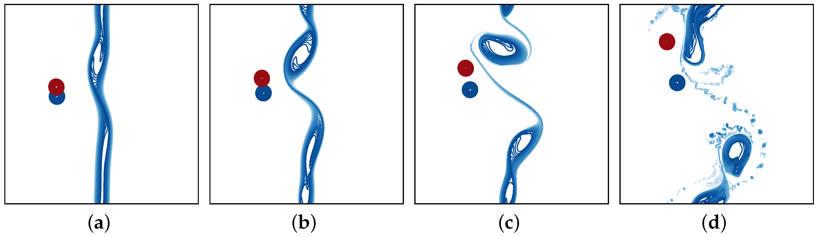
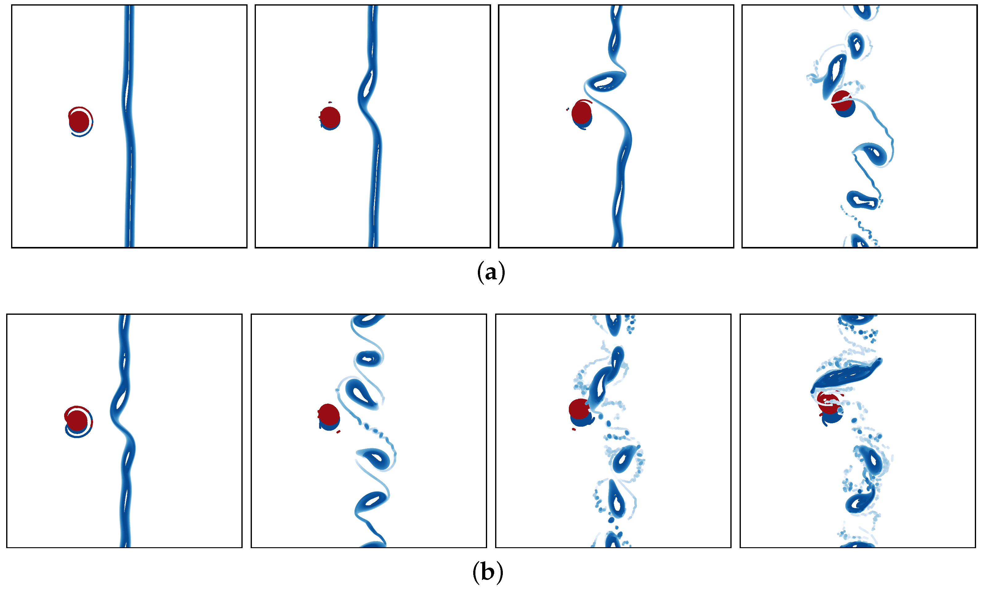
A few times from the flow evolution are presented in Figure 4. As expected, the flow induced by the filament separates the vortices of the heton. The upper, positive vortex moves further towards increasing y, causing the heton to move towards increasing x as found in the idealised model of the previous subsection. The motion of the vortex centres is described in Figure 5. The trajectories show how the upper vortex (vortex 1) separates from the lower vortex (vortex 2). While vortex 2 keeps moving toward and below the filament, vortex 1 eventually pairs up with a counter-rotating surface billow and moves with it toward increasing y. As a result the distance between the vortices increases constantly with time, weakening their interaction. The interaction between the surface billows and the heton also changes the direction of the axis joining the horizontal coordinates of the vortex centres (from the predicted by the idealised model). This increases the deflection of the vortex pair, since the self-induced velocity (albeit weakening) of the vortex pair is perpendicular to this axis. This effect is due to both the destabilisation of the filament and the deformation of the vortex cores.
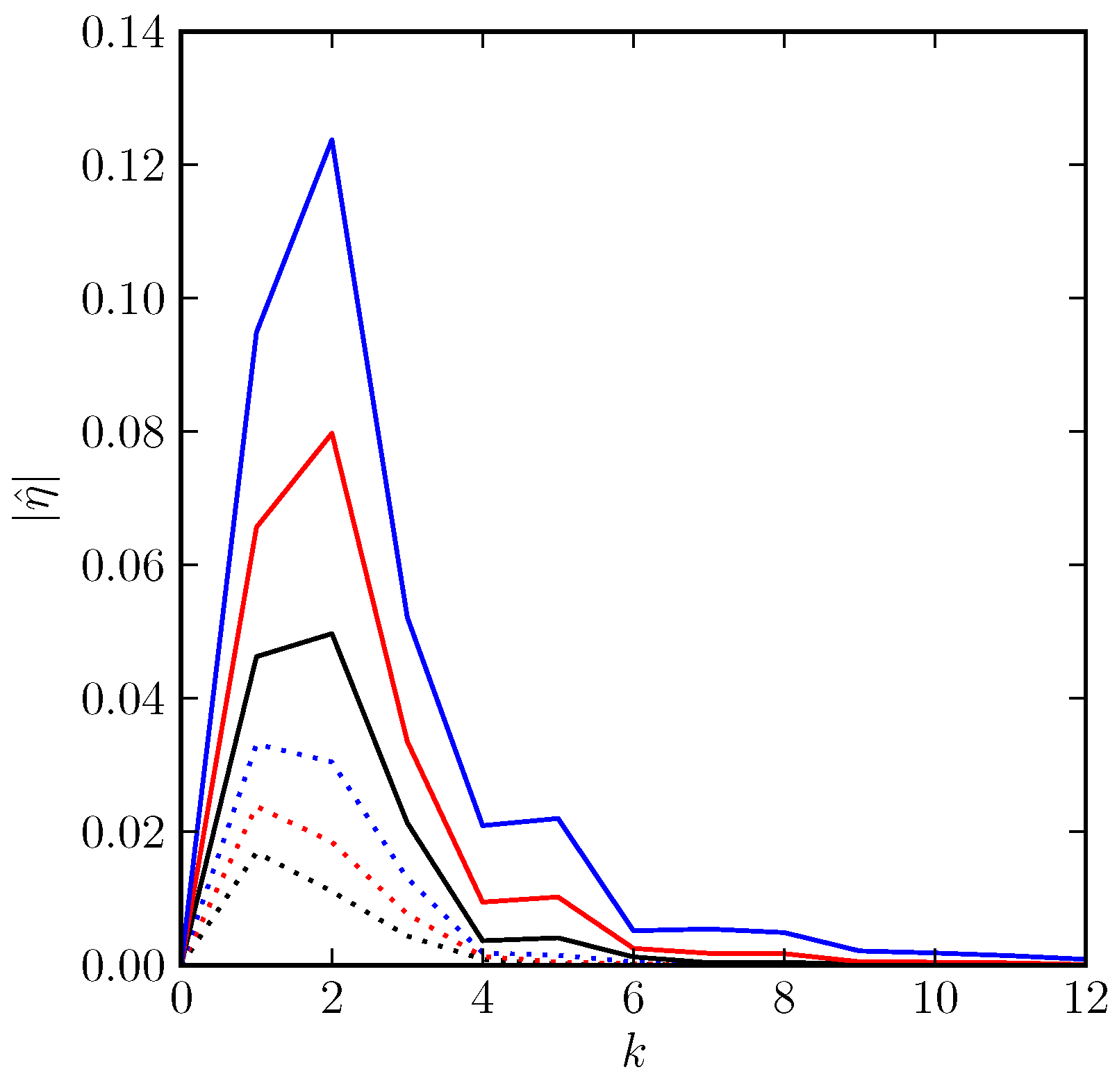
The heton velocity field perturbs the filament, destabilises it, and causes it to break up into a series of billows. As the heton moves towards and along the filament, the induced flow field constantly changes, and this has an impact on the development of the filament instability. The billows are not equally spaced, nor are they similar in shape and size. However, we see that two to three billows form. Notably, a monochromatic mode with wavenumber corresponds to a dimensionless wavenumber , which is close to the value associated with the fastest growing mode on an isolated filament. The heton however does not predominantly excite , but rather , as shown by the spectral analysis presented in Figure 6. After a short period of time, becomes dominant, which may be due to the faster linear growth rate of compared to , but also may in part be due to the constantly changing perturbation induced by the heton and nonlinear interactions. The mode never catches up, despite it being most unstable for an isolated filament. The validity of linear theory breaks down before has a chance to grow appreciably.
At later times, the surface buoyancy field becomes more turbulent though the main billows persist, and continue interacting with the vortices below. Many fine-scale features appear on the surface, characteristic of surface QG turbulence [21]. Note that the earlier evolution is only weakly affected by the periodic boundary conditions imposed on the flow, as shown in the Appendix A. Periodic images of the heton have little impact on the way in which the heton approaches and destabilises the filament.
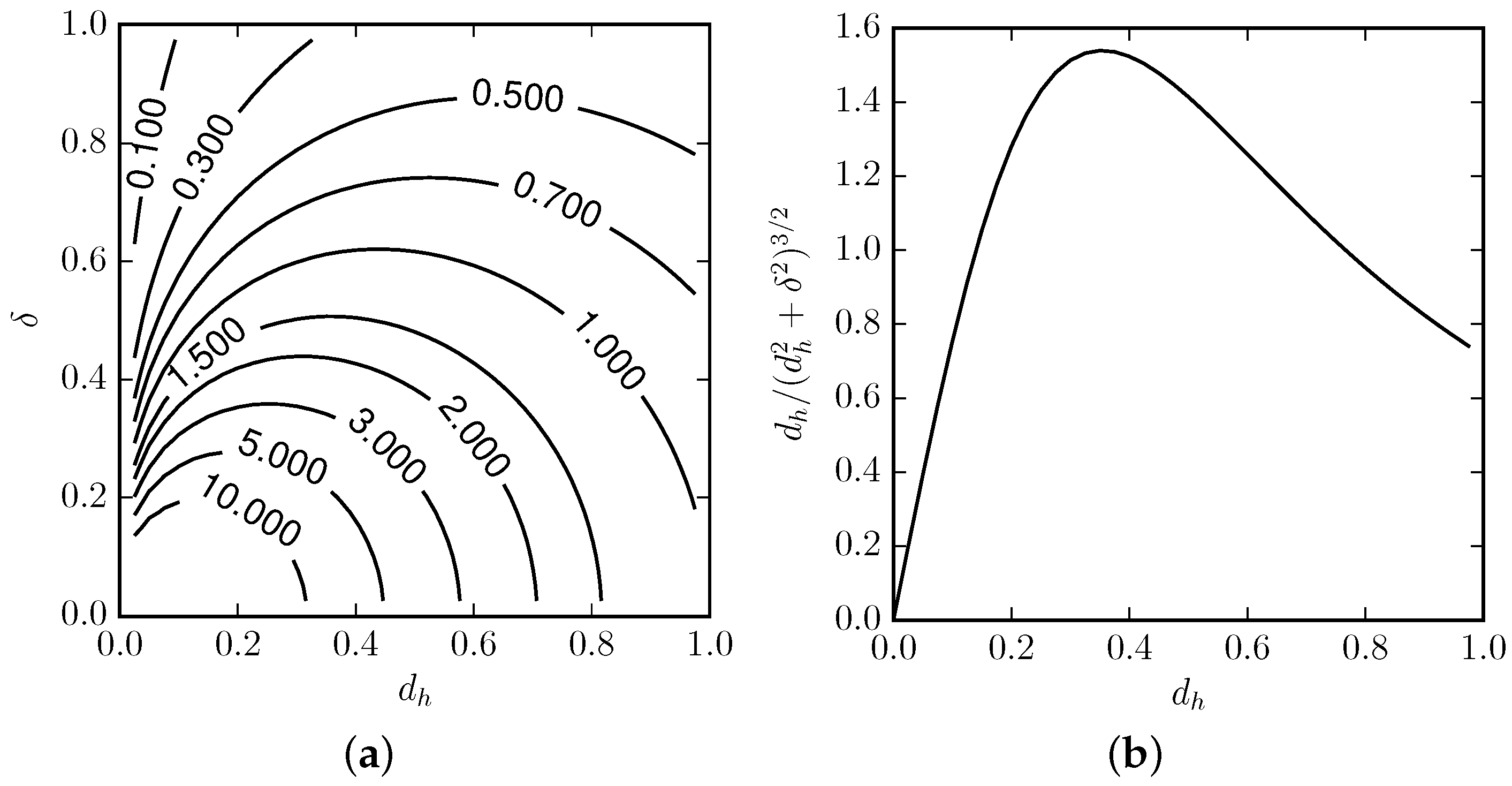
We next examine more widely the influence of the initial flow geometry on the development of the flow. We first focus on the effect of increasing , the vertical separation between the two vortices of the heton. Recall that the translation velocity of a pair of point vortices of opposite strengths is given by:
where is the horizontal distance between the point vortices and is the full three-dimensional distance between them. This means that for a given , increasing d decreases the interaction between the vortices, and therefore decreases their translation velocity. However, in the presence of a surface filament, increasing the vertical offset also increases the difference in velocity induced by the filament on the vortices, and consequently increases the horizontal offset . This in turn increases the translation velocity, at least for . The dependence of on and is summarised in Figure 7.
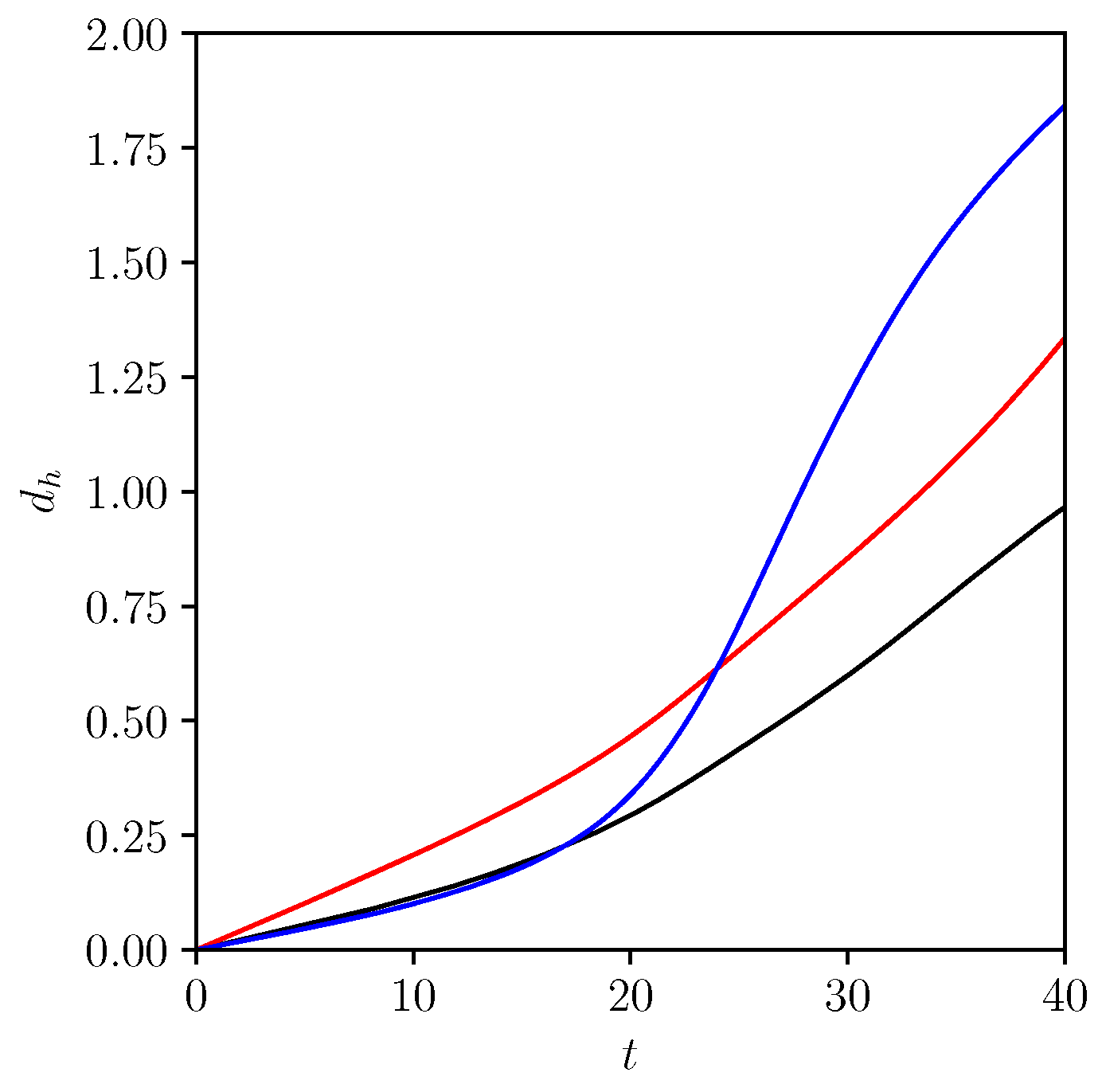
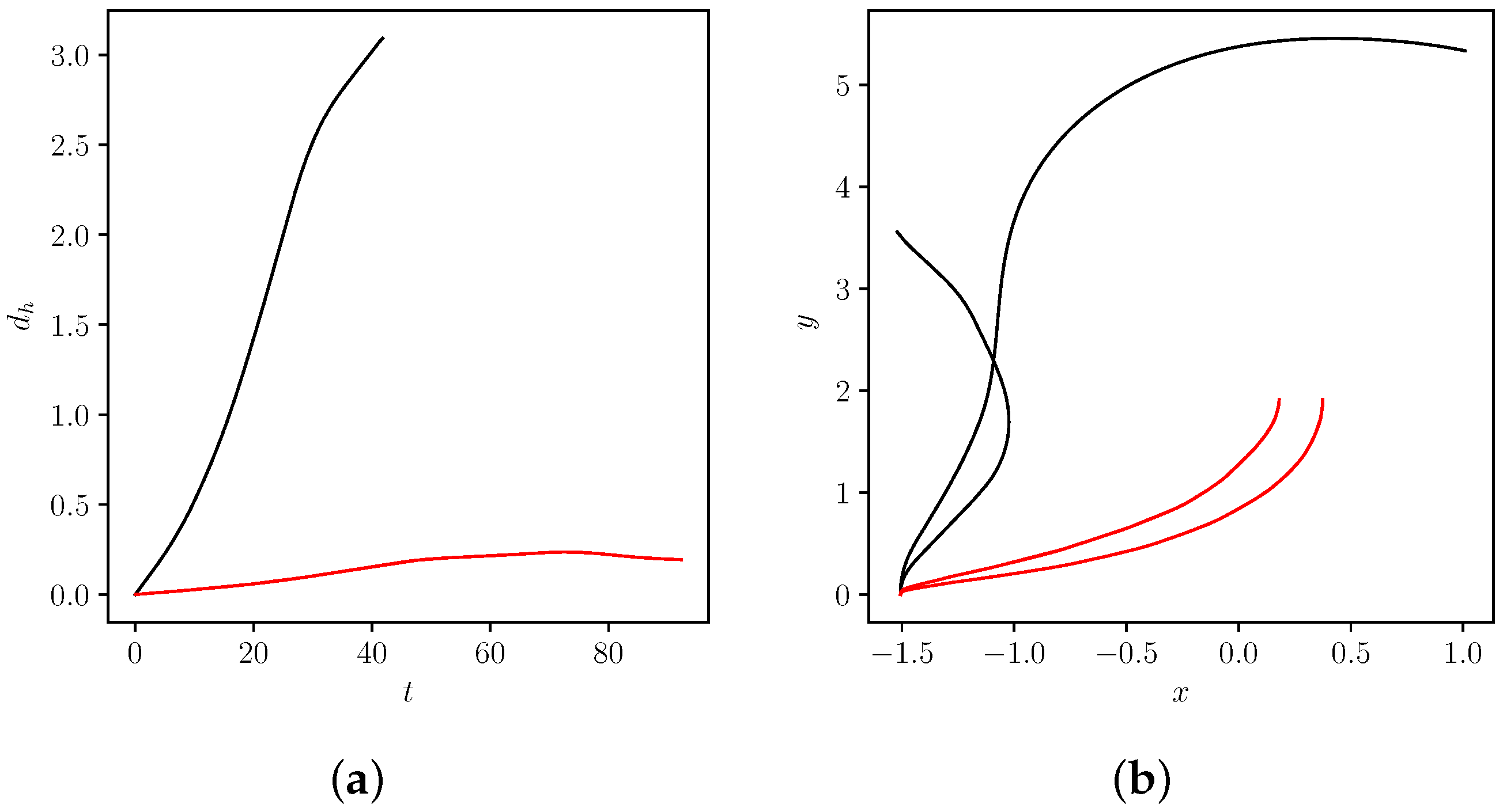
Results for the case , where is doubled relative to case 1 while keeping all other parameters the same, are presented in Figure 8. The main difference is that here the vortices of the heton separate more rapidly, as anticipated. The time evolution of is presented in Figure 9 and compared to case 1 (red and black curves). The wider separation initially speeds up the vortices until this is compensated by the growth in three dimensional distance d. The net effect is that the dipole approaches the filament more slowly in this case.
On the other hand, the early development of the filament instability is very similar. This indicates that, in these cases, the evolution of the filament is mostly driven by its internal dynamics, while the heton mainly acts as a source of perturbations. More pronounced differences between the two cases become apparent at later stages due to nonlinear effects, and in particular when the vortices have become close enough to the filament billows to interact individually with them. At later stages, the interior vortices interact with the surface billows, accelerating the turbulent cascade occurring at the surface.
We next investigate the effect of the mean depth H of the heton by placing the heton closer to the surface. Case is identical to case 1 except the mean depth is decreased from to . Then, the upper vortex almost touches the surface. The flow is illustrated in Figure 10. In this situation, the heton experiences weaker vertical shear coming from the filament, though the magnitude of the velocity is larger. This results in a slower horizontal separation of the two vortices at early times, as seen in Figure 9. Moreover, the heton moves more slowly toward the filament at early times. However, once the filament instability begins to produce billows, the coupling of the upper vortex with one of the billows is enhanced, and the upper vortex separates more rapidly from the lower vortex and pairs instead with a surface billow.
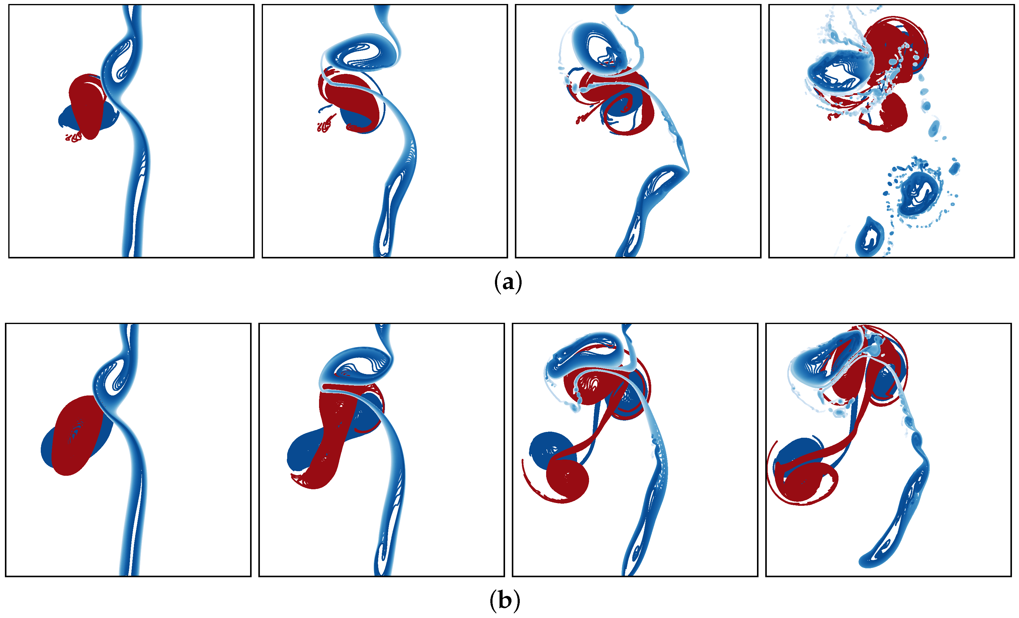
The heton used in the previous experiments is stable in isolation. Wider hetons, with vortices having a larger width-to-height aspect ratio , may be subject to baroclinic instability [15]. The effect of wider hetons is explored in the next two numerical experiments, case where is doubled to 1, and case where is tripled to , keeping all other parameters the same as in case 1. In both of these new cases, the heton is baroclinically unstable to an azimuthal mode 2 deformation. However, when , the instability simply leads to a quasi-periodic oscillation of the vortex between a near circular form and a crossed dumbbell state [15]. Introducing a surface filament adds an extra source of horizontal and vertical shear, and as shown in Figure 11a, this is enough to split the upper vortex of the heton. This upper vortex is wedged between the lower vortex and an upper surface billow, both of which act to increase the deformation on the upper vortex, causing it to split asymmetrically into two main pieces. The lower vortex remains largely intact. In a second case with (Figure 11b), the heton splits into two smaller hetons, one of which pairs with a surface billow while the other moves away. In this case, the heton in isolation would break into two symmetrical hetons [15]. The filament only accelerates the process.
In all cases described thus far, the heton fails to cross below the filament. Once the heton gets close enough to the filament, the upper vortex pairs with a billow formed from the destabilised filament. This new counter-rotating vortex pair moves away, approximately along the y direction, leaving the lower vortex behind and disassociated from other surface structures. The lower vortex hardly moves at late times.
In the next example, case 4, the strength of the filament is weakened compared to that of the vortices, here by reducing ten-fold, from to . Results are presented in Figure 12. In this case, the much weaker vertical shear induced by the filament leads to only a small horizontal offset of the vortices. This slows their mutual propagation speed and keeps them tightly coupled, as shown by the diagnostics in Figure 13. Compared to previous cases, is an order of magnitude smaller. This is expected since the velocity difference is proportional to the strength of the filament. The small offset is nonetheless sufficient to enable to heton to propagate toward the filament, albeit on a much longer timescale. Along the way, the heton is deflected by the large billow formation occurring on the filament, induced by the arriving heton. This rotates the direction of propagation of the heton by more than , and causes it to reverse direction but not before it has crossed below the original location of the filament. Notably, as the heton passes below the filament, it traps part of it and extends the trailing filament, which then is even more unstable [23,32]. This results in the formation of a string of small but intense billows trailing behind the heton.
We now discuss the opposite case of a more intense surface filament, case 5, here with which is 5 times larger than the default case 1. The flow evolution is shown in Figure 14. As expected, the filament destabilises much more rapidly, and billows fully form before the heton reaches the position of the original filament. Because the filament instability occurs on a much shorter time scale than that associated with the heton, the instability is less influenced by heton. This results in a more regular series of billows, here three nearly equal-sized ones, as would be expected for a filament in isolation. Irregularities are primarily due to the time-dependence of the heton-induced perturbations. At late times, the vortices of the heton only weakly interact, and are swept along by the flow field of the surface billows while slowly moving away from each other.
We next examine the joint influence of the width and intensity of the filament. Recall that the buoyancy filament induces a maximum velocity at the surface equal to , while the horizontal shear inside the filament is uniform and equals . Hence, it is possible to increase and a proportionally while leaving the dimensionless horizontal shear unchanged. However, increasing increases the vertical shear experienced by the heton.
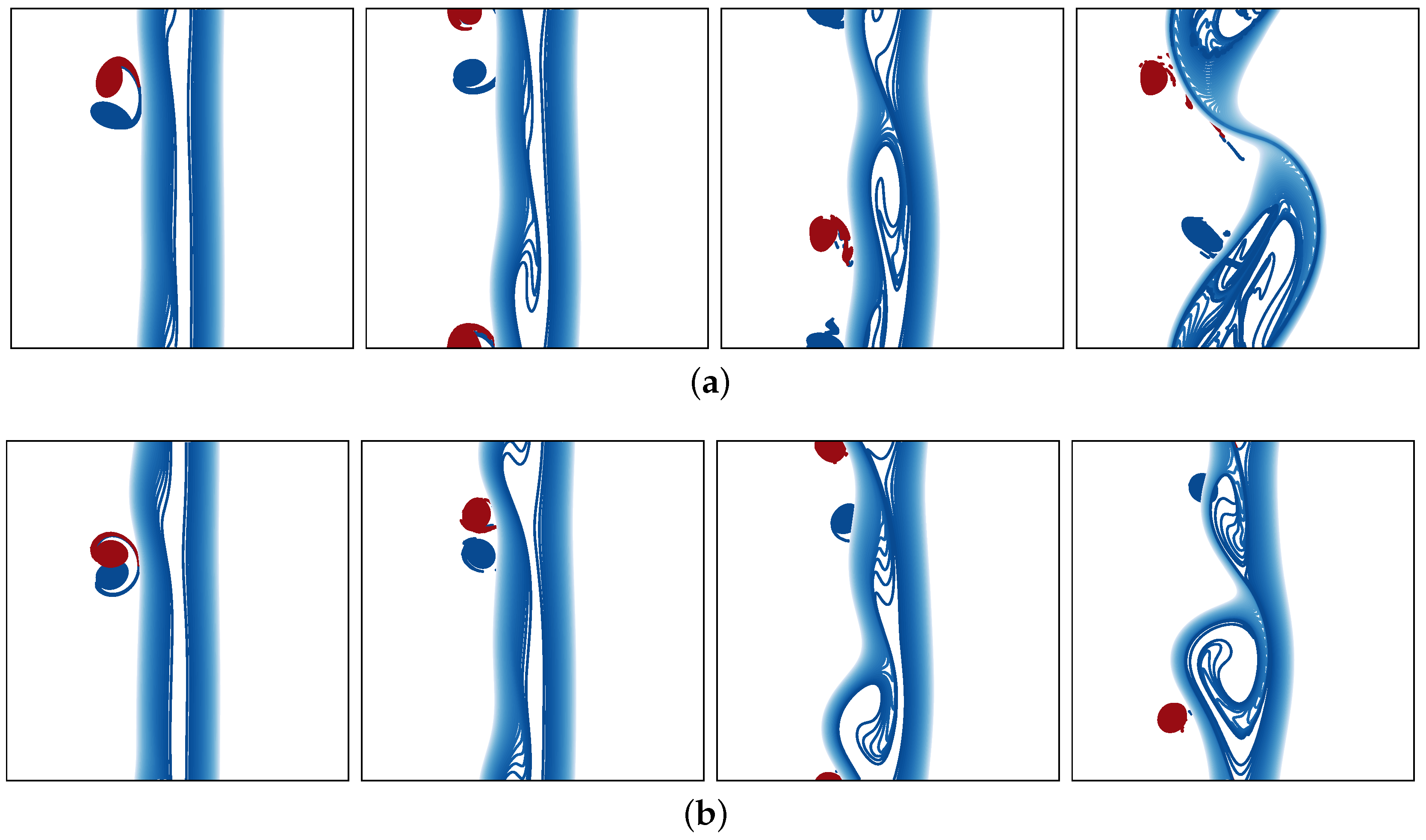
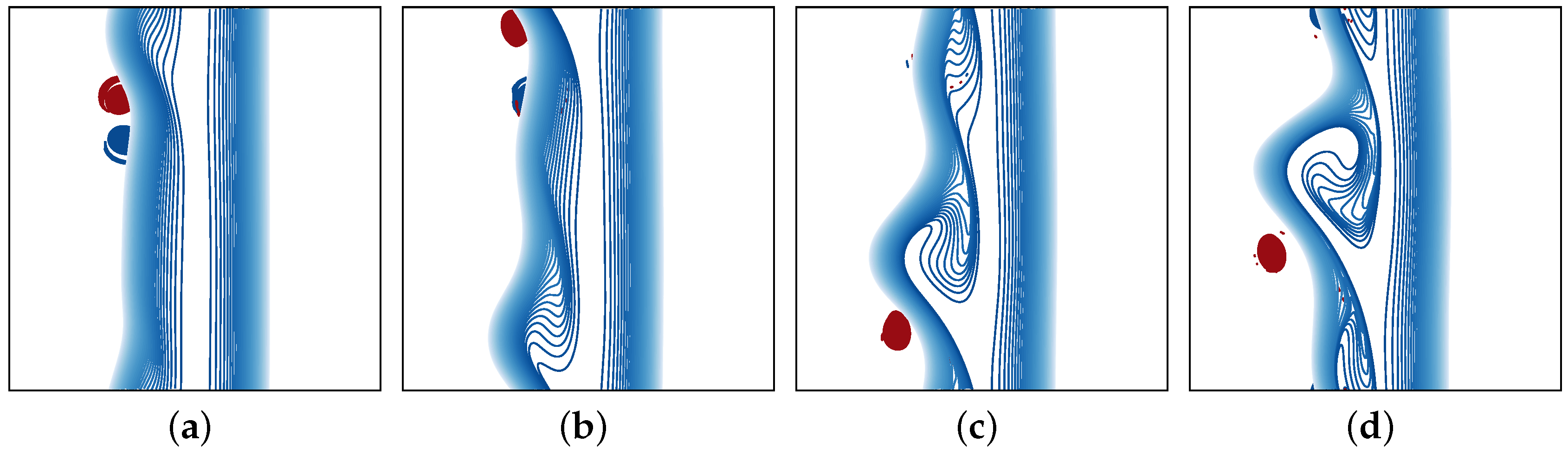
Consider then a filament 3 times wider than the default case, i.e. with . The filament is still unstable in isolation, but only to the wavenumber . Consider further two subcases: with three times larger than in the default case so that is unchanged but the vertical shear is increased; and with the same as in the default case so that is 3 times smaller but the vertical shear is unchanged. These two subcases are contrasted in Figure 15. In both cases, the heton propagates toward the filament and destabilises it, but the nonlinear evolution of the filament is strikingly different. When the horizontal shear is unchanged from the default case (see Figure 15a), the filament develops a mixed and wave disturbance before rolling up into predominantly one large billow. The vertical shear associated with the filament pulls apart the heton, which remains on the outskirts of the developing billow. By contrast, when the vertical shear is weakened by a factor of 3 (Figure 15b), the vortices of the heton separate less rapidly and the filament appears to destabilise mainly on one side. This is partly due to the vortices rolling up the filament in a quasi-passive manner (as discussed further below). The vertical shear associated with the filament still manages to separate the vortices of the heton.
We next contrast these two subcases for wide filaments with two others for thin filaments. Consider then reducing a by a factor of 2 to . In case , we keep the horizontal shear the same as in the default case by reducing (hence reducing the velocity at the filament edges) by a factor of 2, thereby weakening the vertical shear. In case , we increase the horizontal shear by a factor of 2 by leaving unchanged, thereby also leaving the vertical shear unchanged.
These results are shown in Figure 16. Due to the relatively large size of the heton compared to the width of the filament, the heton induces a relatively long wave perturbation on the filament, triggering first a single billow followed by a series of secondary billows. The billows are more regular in case since the filament here is twice as intense. The appearance of approximately five billows is one less than expected from the linear stability analysis of a strip in isolation [23]. A monochromatic wave with wavenumber (corresponding to ) has a growth rate , while wavenumber (corresponding to ) has a slightly large growth rate, . The fact that five billows are formed instead of six can be attributed to scale-selective and time-dependent perturbations induced by the heton.
Notably, the heton remains compact with little separation over the entire period of evolution. The filament flow field is more localised than in the default case, and thus has less overall influence on the heton movement. The heton is still deflected by the billows rolling up on the filament but manages to pass underneath without disruption. The horizontal distance between vortex centres along with their trajectories are shown in Figure 17 for the cases and , contrasting the filament width for fixed horizontal shear. In case for (black curves), the vortices rapidly separate and travel to different parts of the domain. In case for (red curves), the vortices remain close together and gradually turn after passing under the filament. At later times in a lower resolution simulation, the vortices continue to move approximately parallel to the original filament (not shown).
An isolated filament is stable for short waves having [23]. We can therefore stabilise the filament in the doubly-periodic domain considered by taking . While this appears artificial, it may help understand the interaction of a very small heton with a relatively wide filament. To this end, consider a case with , and with increased by a factor of 5 relative to the default case 1 in order to keep the horizontal shear the same. This is referred to as case . Results are shown in Figure 18. One half of the filament remains largely undisturbed while the other half buckles and rolls up mainly in response to the heton velocity field. This case is remarkably similar to case shown in Figure 15b. The filament is not passive and separates the heton, but otherwise the vortices remain intact. The buoyancy field at late times becomes progressively more complex, but without the characteristic billow formation seen in all other cases.
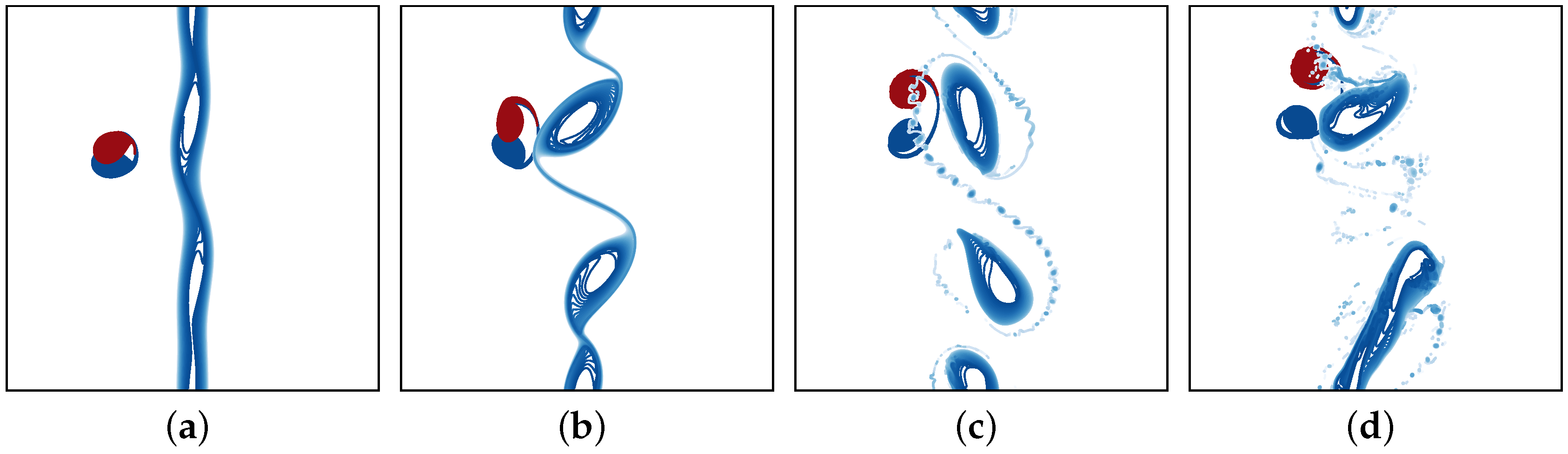
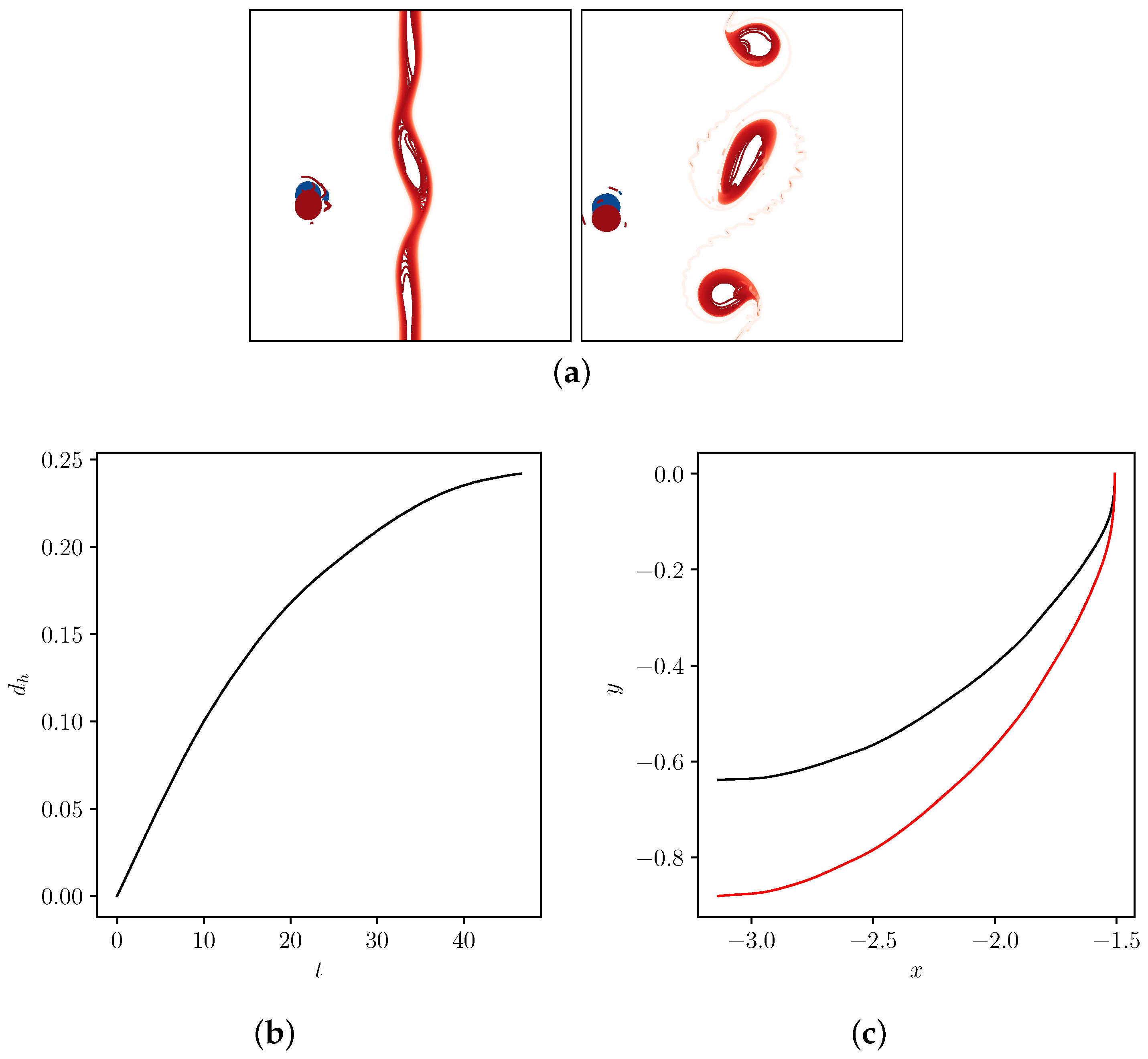
Finally, we examine the interaction of a surface buoyancy filament with a heton whose upper vortex is in cooperative shear with the filament. This case is referred to as case 7 in Table 1, and is shown in Figure 19. The parameters of this case are the same as in the default case 1, apart from the change of sign of the vortex PV. In this case, the vertical shear of the filament separates the vortices and causes them to move away from the filament. The horizontal separation between the vortices tends to a constant, as predicted by the idealised steady filament–point vortex model. The destabilisation of the filament has little influence on the heton behaviour. In contrast with case 1, here the heton’s influence weakens in time and the filament instability is less effected by the heton after receiving its initial perturbation. The filament rolls up into three similar billows, as expected from the linear analysis [23].
4. Conclusions
In this paper, we have presented a detailed analysis of the interaction between a surface buoyancy filament and a heton in the ocean interior. An important factor is the vertical shear induced by the filament. This offsets the two vortices comprising the heton, allowing the heton to move either toward or away from the filament. The heton moves toward the filament if the upper vortex is in adverse shear with the filament; otherwise it moves away. The heton in turn perturbs the filament, which is generally unstable, causing it to roll up into a series of billows. Only when the heton is relatively weak does the filament form regular, evenly-spaced and comparably-sized billows. Otherwise, the heton has a significant impact on the development of the instability. In some cases, the upper half of the heton can pair with a surface billow and move as a vortex pair. In these cases, the heton is separated, and the lower vortex is relatively inactive. In other cases in which the heton is wide enough to be baroclinically unstable, the filament may accelerate the break up of the heton into either smaller hetons or isolated vortices. In general, a heton cannot cross below the filament without being turned around or made to propagate with the surface buoyancy billows.
In summary, this research brings together two important dynamical features of the ocean circulation, namely heat-transporting structures, “hetons”, and variable surface buoyancy. Both features have been analysed extensively in isolation; in combination, they lead to new insights into the motion of hetons and the influence, and dynamics, of surface buoyancy. A key finding here is that subsurface vortices can both induce significant surface flows and alter the evolution of surface buoyancy, indirectly changing the surface flow field.
Author Contributions
Jean Reinaud designed the research, performed the simulations, analysed the results and principally wrote the paper. David Dritschel and Xavier Carton contributed to the design of the research, helped analyse the results and contributed to the writing.
Conflicts of Interest
The authors declare no conflict of interest.
Appendix A. Effect of Periodicity
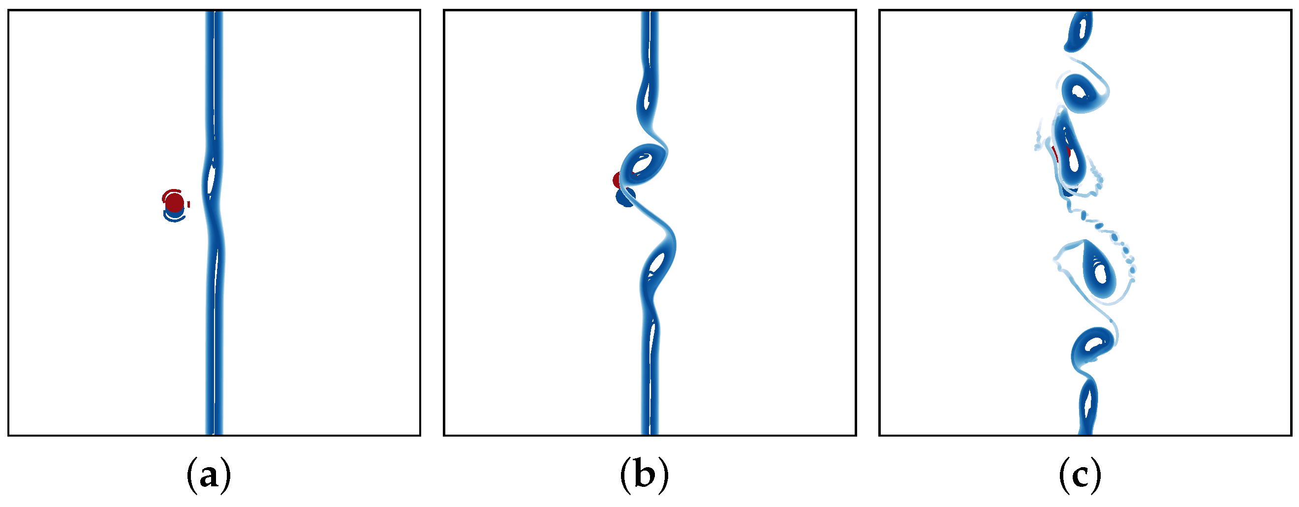
To assess the effect of the horizontally doubly-periodic images of the heton on the flow evolution, we reconsider the geometry of case 1, but in a computational domain effectively twice as large in all three spatial dimensions. We preserve the time scale of evolution by keeping the vortex PV and the filament shear unchanged while reducing all lengths (, etc) by a factor of 2 in the computational box. The distance between the heton and its nearest periodic images is then twice as large, relative to the size of the heton. Notably, as the integral of PV over the heton is zero, the velocity far from the heton decays as the inverse cube of distance. As a consequence, a priori one expects the influence of the periodic images to be small.
This is confirmed by the results presented in Figure A1, which should be compared with the reference case 1 in Figure 4. Up until the time when the heton reaches the filament, the flow evolution in the two cases remains closely similar. The main difference is in the deformation of the portions of the filament furthest from the heton. This is expected, as the far field in the wider computational domain is only periodic on a larger length scale. At late times this affects the flow evolution everywhere, but this is unimportant for understanding the basic characteristics of the interaction of a heton with a buoyancy filament.
Figure A1.
Case similar to case 1 but in a computional domain effectively twice as large. Top view of the flow showing contours of buoyancy and PV at and 40 from (a) to (c).
Figure A1.
Case similar to case 1 but in a computional domain effectively twice as large. Top view of the flow showing contours of buoyancy and PV at and 40 from (a) to (c).

References
- Isern-Fontanet, J.; Lapeyre, G.; Klein, P.; Chapron, B.; Hecht, M. Three-dimensional reconstruction of oceanic mesoscale currents from surface information. J. Geophys. Res. 2008, 113, C09005. [Google Scholar] [CrossRef]
- Wang, J.; Flierl, G.; LaCasce, J.; McLean, J.; Mahadevan, M. Reconstructing the ocean’s interior from surface data. J. Phys. Oceanogr. 2013, 43, 1611–1626. [Google Scholar] [CrossRef]
- Ebbesmeyer, C.C.; Taft, B.A.; McWilliams, J.C.; Shen, C.Y.; Riser, S.C.; Rossby, H.T.; Biscaye, P.E.; Östlund, H.G. Detection, structure and origin of extreme anomalies in a Western Atlantic oceanographic section. J. Phys. Oceanogr. 1986, 16, 591–612. [Google Scholar] [CrossRef]
- Chelton, D.B.; Schlax, M.G.; Samelson, R.M.; de Szoeke, R.A. Global observations of large oceanic eddies. Geophys. Res. Lett. 2007, 34, L15606. [Google Scholar] [CrossRef]
- Chelton, D.B.; Schlax, M.G.; Samelson, R.M. Global observations of nonlinear mesocale eddies. Prog. Oceanogr. 2011, 91, 167–216. [Google Scholar] [CrossRef]
- Zhang, Z.; Wang, W.; Qiu, B. Oceanic mass transport by mesoscale eddies. Science 2014, 345, 322–324. [Google Scholar] [CrossRef] [PubMed]
- Gryanik, V. Dynamics of singular geostrophic vortices in a two-level model of atmosphere (ocean). Izv. Atmos. Ocean. Phys. 1983, 19, 171–179. [Google Scholar]
- Gryanik, V. Dynamics of localized vortex perturbations “vortex charges” in a baroclinic fluid. Izv. Atmos. Ocean. Phys. 1983, 19, 347–352. [Google Scholar]
- Young, W. Some interactions between small numbers of baroclinic, geostrophic vortices. Geophys. Astrophys. Fluid Dyn. 1985, 33, 35–61. [Google Scholar] [CrossRef]
- Hogg, N.; Stommel, H. The heton, an elementary interaction between discrete baroclinic geostrophic vortices and its implications concerning eddy heat flow. Proc. R. Soc. Lond. Ser. A 1985, 397, 1–20. [Google Scholar] [CrossRef]
- Morel, Y.; McWilliams, J. Effect of isopycnal and diapycnal mixing on the stability of oceanic currents. J. Phys. Oceanogr. 2001, 31, 2280–2296. [Google Scholar] [CrossRef]
- Flierl, G.; Xavier, C.; Messager, C. Vortex formation by unstable oceanic jets. Eur. Ser. Appl. Ind. Math. 1999, 7, 137–150. [Google Scholar] [CrossRef]
- Meacham, S. Meander evolution on piecewise-uniform, quasi-geostrophic jets. J. Phys. Oceanogr. 1991, 21, 1139–1170. [Google Scholar] [CrossRef]
- Sokolvskiy, M.; Verron, J. Dynamics of Vortex Structures in a Stratified Rotating Fluid; Springer: Berlin/Heidelberg, Germany, 2014. [Google Scholar]
- Reinaud, J.; Carton, X. The stability and the nonlinear evolution of quasi-geostrophic hetons. J. Fluid Mech. 2009, 636, 109–135. [Google Scholar] [CrossRef]
- Reinaud, J.N. On the stability of continuously stratified quasi-geostrophic hetons. Fluid Dyn. Res. 2015, 47, 035510. [Google Scholar] [CrossRef]
- Gula, J.; Molemaker, M.; McWilliams, J. Submesoscale cold filaments in the Gulf Stream. J. Phys. Oceanogr. 2014, 44, 2617–2643. [Google Scholar] [CrossRef]
- Iermano, I.; Liguori, G.; Iudione, D.; Buongiorno Nardelli, B.; Collela, S.; Zingone, A.; Saggioma, V.; Ribera d’Alcalà, M. Filament formation and evolution in buoyant coastal waters: Observation and modelling. Prog. Oceanogr. 2012, 106, 118–137. [Google Scholar] [CrossRef]
- McWilliams, J.; Gula, J.; Molemaker, M.; Renault, L.; Schchepetkin, A. Filament frontogenesis by boundary layer turbulence. J. Phys. Oceanogr. 2014, 45, 1988–2005. [Google Scholar] [CrossRef]
- Juckes, M. Instability of surface and upper-tropospheric shear lines. J. Atmos. Sci. 1995, 52, 3247–3262. [Google Scholar] [CrossRef]
- Scott, R. A scenario for finite-time singularity in the quasigeostrophc model. J. Fluid Mech. 2011, 687, 492–502. [Google Scholar] [CrossRef]
- Scott, R.; Dritschel, D. Numerical simulation of a self-similar cascade of filament instabilities in the surface quasigeostrophic system. Phys. Rev. Lett. 2014, 112, 144505. [Google Scholar] [CrossRef] [PubMed]
- Reinaud, J.; Dritschel, D.; Carton, X. Interaction between a surface quasi-geostrophic buoyancy filament and an internal vortex. Geophys. Astrophys. Fluid Dyn. 2016, 110, 464–490. [Google Scholar] [CrossRef]
- Ryzhov, E.; Koshel, K.; Carton, X. Passice scalar advection in the vicinity of two point vortices in a deformation flow. Eur. J. Mech. 2012, 34, 121–130. [Google Scholar] [CrossRef]
- Bell, G. Interaction between vortices and waves in a simple model of geophysical flow. Phys. Fluids A Fluids Dyn. 1990, 2, 575–586. [Google Scholar] [CrossRef]
- Bell, G.; Pratt, L. The interaction of an eddy with an unstable jet. J. Phys. Oceanogr. 1992, 22, 1229–1244. [Google Scholar] [CrossRef]
- Dijkstra, H. Dynamical Oceanography; Springer-Verlag: Berlin/Heidelberg, Germany, 2008. [Google Scholar]
- Vallis, G. Atmospheric and Oceanic Fluid Dynamics: Fundamentals And Large-Scale Circulation; Cambridge University Press: Cambridge, UK, 2006. [Google Scholar]
- Dritschel, D.; Ambaum, M. A contour-advective semi-Lagrangian numerical algorithm for simulating fine-scale conservative dynamical fields. Q. J. R. Meteorol. Soc. 1997, 123, 1097–1130. [Google Scholar] [CrossRef]
- Perrot, X.; Reinaud, J.; Carton, X.; Dritschel, D. Homostrophic vortex interaction under external strain in a coupled QG-SQG model. Regul. Chaotic Dyn. 2010, 15, 66–83. [Google Scholar] [CrossRef]
- Dritschel, D. Contour surgery: A topological reconnection scheme for extended integrations using contour dynamics. J. Comput. Phys. 1988, 77, 240–266. [Google Scholar] [CrossRef]
- Harvey, B.; Ambaum, M. Instability of surface-temperature filaments in strain and shear. Q. J. R. Meteorol. Soc. Part B 2010, 136, 1506–1513. [Google Scholar] [CrossRef]
- Dritschel, D. On the stabilization of a two-dimensional vortex strip by adverse shear. J. Fluid Mech. 1989, 206, 193–211. [Google Scholar] [CrossRef]
- Legras, B.; Dritschel, D. Vortex stripping and the generation of high vorticity gradients in two-dimensional flows. Appl. Sci. Res. 1993, 51, 445–455. [Google Scholar] [CrossRef]
- Trieling, R.; Dam, C.; van Heijst, G. Dynamics of two identical vortices in linear shear. Phys. Fluids 2010, 22, 117104. [Google Scholar] [CrossRef]
Figure 1.
Geometry of the initial flow configuration and definition of the parameters. (a) top () view; (b) side () view.
Figure 1.
Geometry of the initial flow configuration and definition of the parameters. (a) top () view; (b) side () view.

Figure 2.
Dimensionless velocity profiles associated with an undisturbed surface buoyancy filament of half-width . (a) surface flow at ; (b) flows at the depths of the upper vortex (, black curve) and the lower vortex (, red curve).
Figure 2.
Dimensionless velocity profiles associated with an undisturbed surface buoyancy filament of half-width . (a) surface flow at ; (b) flows at the depths of the upper vortex (, black curve) and the lower vortex (, red curve).

Figure 3.
(a) trajectories of two point vortices with , and predicted by the simplified model for a fixed filament with and . Vortex 1 is shown by the black curve while vortex 2 is shown by the red curve; (b) horizontal distance between the vortices versus time t.
Figure 3.
(a) trajectories of two point vortices with , and predicted by the simplified model for a fixed filament with and . Vortex 1 is shown by the black curve while vortex 2 is shown by the red curve; (b) horizontal distance between the vortices versus time t.

Figure 4.
Case 1: top view of the flow showing contours of buoyancy and potential vorticity (PV) at , 57 from (a) to (d).
Figure 4.
Case 1: top view of the flow showing contours of buoyancy and potential vorticity (PV) at , 57 from (a) to (d).

Figure 5.
Case 1: trajectories of the vortex centres (vortex 1 in black, vortex 2 in red); horizontal distance between the vortex centres versus time t; and angle between the axis joining the vortices centres and the x axis.
Figure 5.
Case 1: trajectories of the vortex centres (vortex 1 in black, vortex 2 in red); horizontal distance between the vortex centres versus time t; and angle between the axis joining the vortices centres and the x axis.

Figure 6.
Case 1: magnitude of the Fourier modes of deformation of the buoyancy filament at (dotted black), (dotted red), 15 (dotted blue), (solid black), 20 (solid red), (solid blue). The modes are obtained by expressing the displacement of each buoyancy contour from its initial position as a Fourier series in y. The magnitude for each k is defined as the r.m.s. value of over all contours.

Figure 7.
Contours of in the () parameter space; vs for .

Figure 8.
Case : effect of doubling the vertical offset between the two vortices of the heton. Top view of the flow showing contours of buoyancy and PV at and 40 from (a) to (d).
Figure 8.
Case : effect of doubling the vertical offset between the two vortices of the heton. Top view of the flow showing contours of buoyancy and PV at and 40 from (a) to (d).

Figure 9.
Time evolution of the horizontal distance between vortex centres, , for the reference case 1 (black), the case with doubled vertical offset or case (red), and a third case (blue) in which the mean depth of the two vortices is approximately halved, , while keeping all other parameters the same as in case 1.

Figure 10.
Case : effect of decreasing the mean depth H of the heton from to . Top view of the flow showing contours of buoyancy and PV at and 40 from (a) to (d).
Figure 10.
Case : effect of decreasing the mean depth H of the heton from to . Top view of the flow showing contours of buoyancy and PV at and 40 from (a) to (d).

Figure 11.
Cases (a) and (b): effect of increasing the width-to-height aspect ratio of the heton. In case , and , while in case , and , representing a doubling and a tripling relative to the default case 1. Top view of the flow showing contours of buoyancy and PV. In (a), the times shown are and 40, while in (b), the times shown are and 24.

Figure 12.
Case 4: effect of weakening the strength of the filament. Here , ten times smaller than in the default case 1, keeping all other parameters the same. Top view of the flow showing contours of buoyancy and PV at and 160 from (a) to (d).
Figure 12.
Case 4: effect of weakening the strength of the filament. Here , ten times smaller than in the default case 1, keeping all other parameters the same. Top view of the flow showing contours of buoyancy and PV at and 160 from (a) to (d).

Figure 13.
Case 4: trajectories of the vortex centres (vortex 1 in black, vortex 2 in red); horizontal distance between the vortex centres versus time t; and angle between the axis joining the vortices centres and the x axis.
Figure 13.
Case 4: trajectories of the vortex centres (vortex 1 in black, vortex 2 in red); horizontal distance between the vortex centres versus time t; and angle between the axis joining the vortices centres and the x axis.

Figure 14.
Case 5: effect of increasing the strength of the filament. Here , which is 5 times larger than in the default case 1, keeping all other parameters the same. Top view of the flow showing contours of buoyancy and PV at and 11 from (a) to (d).
Figure 14.
Case 5: effect of increasing the strength of the filament. Here , which is 5 times larger than in the default case 1, keeping all other parameters the same. Top view of the flow showing contours of buoyancy and PV at and 11 from (a) to (d).

Figure 15.
Cases (a) and (b): effect of tripling the filament half-width a from to . The dimensionless horizontal shear remains in case while it is reduced by a factor of 3 in case , with all other parameters the same as in case 1. Top view of the flow showing contours of buoyancy and PV. In (a), the times shown are and 32, while in (b), the times shown are and 36.

Figure 16.
Cases (a) and (b): effect of halving the filament half-width a from to . The dimensionless horizontal shear remains in case while it is increased by a factor of 2 in case , with all other parameters the same as in case 1. Top view of the flow showing contours of buoyancy and PV. In (a), the times shown are and 50, while in (b), the times shown are and 33.

Figure 17.
(a) horizontal distance between the vortex centres versus time t for case (wide filament, black) and case (thin filament, red); (b) trajectories of the vortex centres (same colour coding).
Figure 17.
(a) horizontal distance between the vortex centres versus time t for case (wide filament, black) and case (thin filament, red); (b) trajectories of the vortex centres (same colour coding).

Figure 18.
Case : effect of a very wide filament, , which is linearly stable in isolation. Here is increased in proportion to a to keep the same as in the default case 1. Top view of the flow showing contours of buoyancy and PV at and from (a) to (d).
Figure 18.
Case : effect of a very wide filament, , which is linearly stable in isolation. Here is increased in proportion to a to keep the same as in the default case 1. Top view of the flow showing contours of buoyancy and PV at and from (a) to (d).

Figure 19.
Case 7: effect of reversing the vortex PV. All parameters are otherwise the same as in the default case 1. (a) top view of the flow showing contours of buoyancy and PV at and 36 from left to right; (b) horizontal distance between the vortices versus time; (c) trajectories of the vortex centres.


Table 1.
Summary of the high resolution nonlinear simulations performed.
| Case | |||||
|---|---|---|---|---|---|
| 1 (ref) | 4 | 1 | 1 | ||
| 4 | 2 | 1 | |||
| 1 | 1 | ||||
| 4 | 1 | 1 | 2 | ||
| 4 | 1 | 3 | |||
| 4 | 4 | 1 | 1 | ||
| 5 | 4 | 2 | 1 | 1 | |
| 1 | |||||
| 1 | |||||
| 8 | 1 | 2 | |||
| 8 | 1 | 2 | |||
| 1 | |||||
| 7 | 4 | 1 | 1 |
© 2017 by the authors. Licensee MDPI, Basel, Switzerland. This article is an open access article distributed under the terms and conditions of the Creative Commons Attribution (CC BY) license (http://creativecommons.org/licenses/by/4.0/).
Share and Cite
MDPI and ACS Style
Reinaud, J.N.; Carton, X.; Dritschel, D.G. Interaction between a Quasi-Geostrophic Buoyancy Filament and a Heton. Fluids 2017, 2, 37. https://doi.org/10.3390/fluids2030037
AMA Style
Reinaud JN, Carton X, Dritschel DG. Interaction between a Quasi-Geostrophic Buoyancy Filament and a Heton. Fluids. 2017; 2(3):37. https://doi.org/10.3390/fluids2030037
Chicago/Turabian StyleReinaud, Jean N., Xavier Carton, and David G. Dritschel. 2017. "Interaction between a Quasi-Geostrophic Buoyancy Filament and a Heton" Fluids 2, no. 3: 37. https://doi.org/10.3390/fluids2030037