Particulate Levels Underneath Landscape Fire Smoke Plumes in the Sydney Region of Australia


1
Bushfire Risk Management Research Hub, University of Wollongong, Wollongong, NSW 2522, Australia
2
Hawkesbury Institute, Western Sydney University, Penrith, NSW 2751, Australia
*
Author to whom correspondence should be addressed.
Fire 2023, 6(3), 86; https://doi.org/10.3390/fire6030086
Submission received: 24 December 2022
/
Revised: 14 February 2023
/
Accepted: 21 February 2023
/
Published: 24 February 2023
Abstract
:Smoke pollution from landscape fires is a major health problem, but it is difficult to predict the impact of any particular fire. For example, smoke plumes can be mapped using remote sensing, but we do not know how the smoke is distributed in the air-column. Prescribed burning involves the deliberate introduction of smoke to human communities but the amount, composition, and distribution of the pollution may be different to wildfires. We examined whether mapped plumes produced high levels of particulate pollution (PM2.5) at permanent air quality monitors and factors that influenced those levels. We mapped 1237 plumes, all those observed in 17 years of MODIS imagery over New South Wales, Australia, but this was only ~20% of known fires. Prescribed burn plumes tended to occur over more populated areas than wildfires. Only 18% of wildfire plumes and 4% of prescribed burn plumes passed over a monitor (n = 115). A minority of plumes caused a detectable increase in PM2.5: prescribed burn plumes caused an air quality exceedance for 33% of observations in the daytime and 11% at night, wildfire plumes caused exceedances for 48% and 22% of observations in the day and night-time, respectively. Thus, most plumes remained aloft (did not reach the surface). Statistical modelling revealed that wind speed, temperature, and mixing height influenced whether a plume caused an exceedance, and there was a difference between prescribed and wild fires. In particular, in wind speeds below 1 kmhr−1, exceedance was almost certain in prescribed burns. This information will be useful for planning prescribed burning, preparing warnings, and improving our ability to predict smoke impacts.
1. Introduction
Wildfires cause a range of direct and indirect impacts on human values. It is becoming increasingly clear that the impact of smoke from wildfires can be at least equal to the direct costs of the fires themselves [1]. For example, it has been estimated that 340,000 people die every year from the effects of wildland [2]. Moreover, wildfire area has been increasing in recent years in California and Australia [3,4], and this has been associated with enormous poor air quality events [1] which will become worse [5].
In all fire-prone areas around the world, fire managers implement strategies to reduce the direct impact of fires, but there has been little attention to the consequences in terms of impacts on smoke exposure [2]. The most important issue in this regard is the widespread use of prescribed burning to hinder the spread of wildfire [6]. Prescribed burning is the deliberate application of the landscape to achieve some goal, most commonly reducing the fuel available for wildfires [7]. Prescribed burning has caused poor air-quality events in many instances around the world [8,9,10], and indeed it is the biggest source of particulate matter in the southern USA [11]. It has also been linked to elevated health problems in areas with high levels of prescribed burning [12]. Prescribed burning reduces the area of wildfire, and this “Leverage” has been quantified for many regions around the world. In almost all of these regions, prescribed burning causes an increase in the overall area burnt [13], though the total amount of fuel consumed and hence the emissions produced may not increase [14]. Another potential problem with prescribed burns is that they generally occur closer to populated centres than do wildfires [15], precisely because their primary purpose is to protect those centres. On the other hand, prescribed fires usually burn at a lower intensity, consume less fuel, and, hence, produce less smoke per ha burnt than wildfires. Moreover, managers can choose to implement prescribed burns when the atmospheric conditions are suitable to carry the smoke away from populated areas. These many and sometimes countervailing factors raise the important question of whether prescribed burning causes a net increase or decrease in population exposure to smoke pollutants [6].
Answering this question is difficult. There is a general lack of understanding about the fate of smoke from landscape fires (wildfire or prescribed) [10]. This is partly because smoke is a dynamic and spatiotemporal phenomenon whereas our systems for monitoring air quality are small in number and are static. It is also partly because it is hard to identify landscape fires as the source of air pollution, especially in an urban setting, though there have been attempts to identify wood smoke [16]. Empirical studies that measure spatial patterns of pollution from individual fires are rare, and those focussing on prescribed burns are even rarer [9,17]. Physically-based smoke dispersion models are continually improving and are routinely used to forecast air quality at regional scales and for specific events, including individually prescribed burns [18]. However, these models operate on grid cells ranging from 1 to 10 km depending on the application, which is too large to capture local effects from smoke plumes. Validation studies suggest that the correlation between regional-scale forecast models and actual pollution levels is about 0.4 [19], while event-scale models may fail to capture important events such as temperature inversions responsible for high levels of smoke pollution [20].
There is a need to gather empirical data on the dispersion of smoke from individual landscape fires in order to understand the contribution of fire to air quality, and to validate existing models and contribute to their improvement so that vulnerable people can be better forewarned of likely smoke impacts. There are a variety of methods that could be used. One is to deploy pollution monitors around fires (as in [9]), while another is to attempt to identify the signature of individual fires on the permanent air quality network. The approach we take in this study was to match remotely sensed observations of smoke plumes to data from a permanent air quality monitoring network. Plumes can be observed via a range of remote sensing methods and can be mapped. This is done by hand digitization of plumes, routinely for the entire USA by the HMS program [21] and for specific research projects elsewhere [22]. However, it is not known how the observed plume affects air quality on the ground where people are exposed. In particular, remotely sensed plumes may be lofted well above the ground and so have little impact on people.
Improving knowledge and the modelling of landscape fire smoke can serve many purposes:
Real-time measurement and monitoring of air quality (AQ) to estimate regional exposure, which is primarily through an extensive network of monitors, but also via methods to interpolate AQ between them [23,24].
Forecasting to provide timely warnings, which involves either empirical or physical models to predict AQ as a function of fire and atmospheric conditions [19,25,26]. This involves continual model development, improvement, and validation via reference to actual observations.
Improving management decisions to reduce impacts from prescribed burning, essentially asking: what is the risk of a poor AQ event if I light a prescribed burn there now or tomorrow?
Our study is primarily directed at the latter, though it also helps to inform other endeavours. We mapped all of the plumes observable from remote sensing for a 17-year period and investigated their temporal and spatial patterns, impact on air quality, and meteorological conditions that could predict poor air quality beneath them. Specifically, the aims were to:
- Determine the proportion of fires that create observable plumes.
- Describe the spatial and temporal patterns in plumes (spatial and monthly hotspots for plumes).
- Determine the population densities of the places that plumes pass over (the human dimension of the problem).
- Determine what proportion of plumes pass over an air quality monitor (adequacy of the network).
- Determine what proportion of plumes cause a poor air quality incident.
- Investigate meteorological conditions associated with those incidents to improve forecast ability.
In each of these aims, we also investigated differences between wildfires and prescribed fires.
2. Materials and Methods
2.1. Datasets
The fire history for NSW was downloaded from the NSW Government spatial data portal (DPE unpublished data, https://www.seed.nsw.gov.au (accessed on 23 December 2022)). This contains the perimeter and dates for all fires (though some dates are missing). A 1 km resolution human population grid was obtained from the Australian Bureau of Statistics based on the 2011 census (https://www.abs.gov.au/ausstats/[email protected]/mf/1270.0.55.007 (accessed on 23 December 2022)). The NSW Government (Department of Planning and Environment) maintains a network of compliance standard air quality monitors, that has gradually expanded over the years from seven monitors recording PM2.5 in 2003 to 36 by 2020 [27]. They provided us with data for hourly particulate matter of <2.5 microns (PM2.5) from 26 of these monitors (those with the longest duration). We used data starting in 2002 to coincide with the plumes data (see below). We obtained hourly weather data from the Bureau of Meteorology (BOM) to extract the weather from the closest monitoring station to the air quality monitor. Lastly, we obtained six am upper atmospheric radiosonde data from the Sydney Airport BOM station from which we extracted or calculated surface pressure (in Hectopascals), mixing height, and inversion height. Inversion height is the height above the surface (in m) at which the atmosphere begins to cool with altitude and mixing height is the height below which air is turbulently mixed [28]. Inversion height and mixing height are related concepts, but are not closely correlated in our data (r = 0.21).
Plumes were hand digitized in a GIS platform for an area within 250 km of Sydney, in which all of the air quality monitors occur. For the period from mid 2013 to January 2020, we used the fire history data to identify days and locations where plumes could potentially have occurred. We then examined true colour satellite images from the MODIS Terra (approx. 10:30 overpass time) and Aqua satellite (approx. 14:30 overpass time) in the NASA Worldview website (www.worldview.earthdata.nasa.gov (accessed on 23 December 2022)), cross-referencing them to the fire history. Where an obvious plume or smoke haze was visible, the image was downloaded and overlaid on the fire history in ArcMap 10 GIS. The plume boundary was digitized onto the image, the area of the plume was calculated and the plume was tagged to the fire that caused it. Some fires caused plumes on multiple days and these were all digitized. The method was similar to the ongoing MODIS-based program applied to the USA in the national smoke plume mapping system HMS [21]. We also made use of data from two previous studies. Williamson, Price, Henderson, and Bowman [22] digitized 133 plumes using a similar method to ours from December 2003 to mid-2009. Price et al. [29] digitized 103 plumes from Bureau of Meteorology radar data for the period mid-2009 to December 2013.
2.2. Analysis
We compared the number of fires in the fire history database to the number of plumes mapped to estimate the proportion of fires of different types that produced detectable plumes. We also explored the distribution of plumes of each fire type according to plume area, year, and calendar month. In a GIS, we overlaid and combined the plumes to produce a raster of plume frequency for prescribed and wildfires separately. We intersected each plume frequency grid with the 1 km census population grid, and then examined the distribution of population number for cells exposed to 1–3 plumes and more than three plumes, considering prescribed and wildfires separately.
We used the GIS to intersect the plumes with the air quality monitors to create a sample of observations where a plume passed over a monitor. Each plume had as many observations as monitors it covered, with the maximum being five. For each of these observations, we calculated the mean PM2.5 value at the monitor for a three-hour-period centered at 2 pm (the approximate time of the daily Aqua satellite overpass which detected most of the plumes). Empirical evidence suggests that prescribed burn plumes sometimes collapse at night, causing an increase in ground-level particulates [9], so we also calculated the mean PM2.5 for the three hours centered on 4 am during the following night. Due to the fact that not all poor air quality events are due to fires, we attempted to eliminate these by examining the air quality on the previous day. The PM2.5 measurements were complimented by calculating the PM2.5 for the same three hours from the previous day, and the previous night. For daytime, we defined a poor air quality exceedance event as where the three-hour mean was >25 μgm−3 and higher than the previous day. For night-time, there were only three exceedances for prescribed burns, so for the statistical model, we used a lower threshold of 18 μgm−3 for night-time: using this definition there were eight exceedances.
Then, we applied binomial regression modeling to associate poor air quality events with atmospheric conditions (see Table 1 for a description of the variables). We modelled day and night times separately, for the reasons mentioned above. For the nighttime, the predictors were the same as for daytime except the weather variables were calculated for the night period, though for the following morning in the case of surface pressure, mixing height, and inversion height, because since night-time values are not recorded for those variables. All combinations of the predictor variables were fitted and the best model was determined using model selection techniques, selecting the model with the lowest Akaike’s Information Criteria (AIC) value (Burnham et al., 2002). Then, we tested whether any of the selected predictors had an interaction with fire type and retained those that reduced AIC. These observations were dominated by plumes from the 2019-20 Black Summer bushfire seasons, both because there were many plumes and because they tended to cover many air quality monitors. To test whether the effects in the main model were consistent across seasons, we repeated the model fitting for both day and nighttime observations excluding the 2019-20 wildfires. There were only 74 valid observations for these models so it was not expected that they would contain as many variables as the complete models.
3. Results
We identified and digitized 972 plumes altogether, comprising 484 from prescribed and 488 from wildfires. Seventy-seven plumes were duplicates (more than one day for the same fire): two prescribed and seventy-five wildfires. In this 250 km zone around Sydney, the fire history contained 1901 prescribed and 2835 wildfires, so 25.4% and 14.6% produced detectable plumes, respectively.
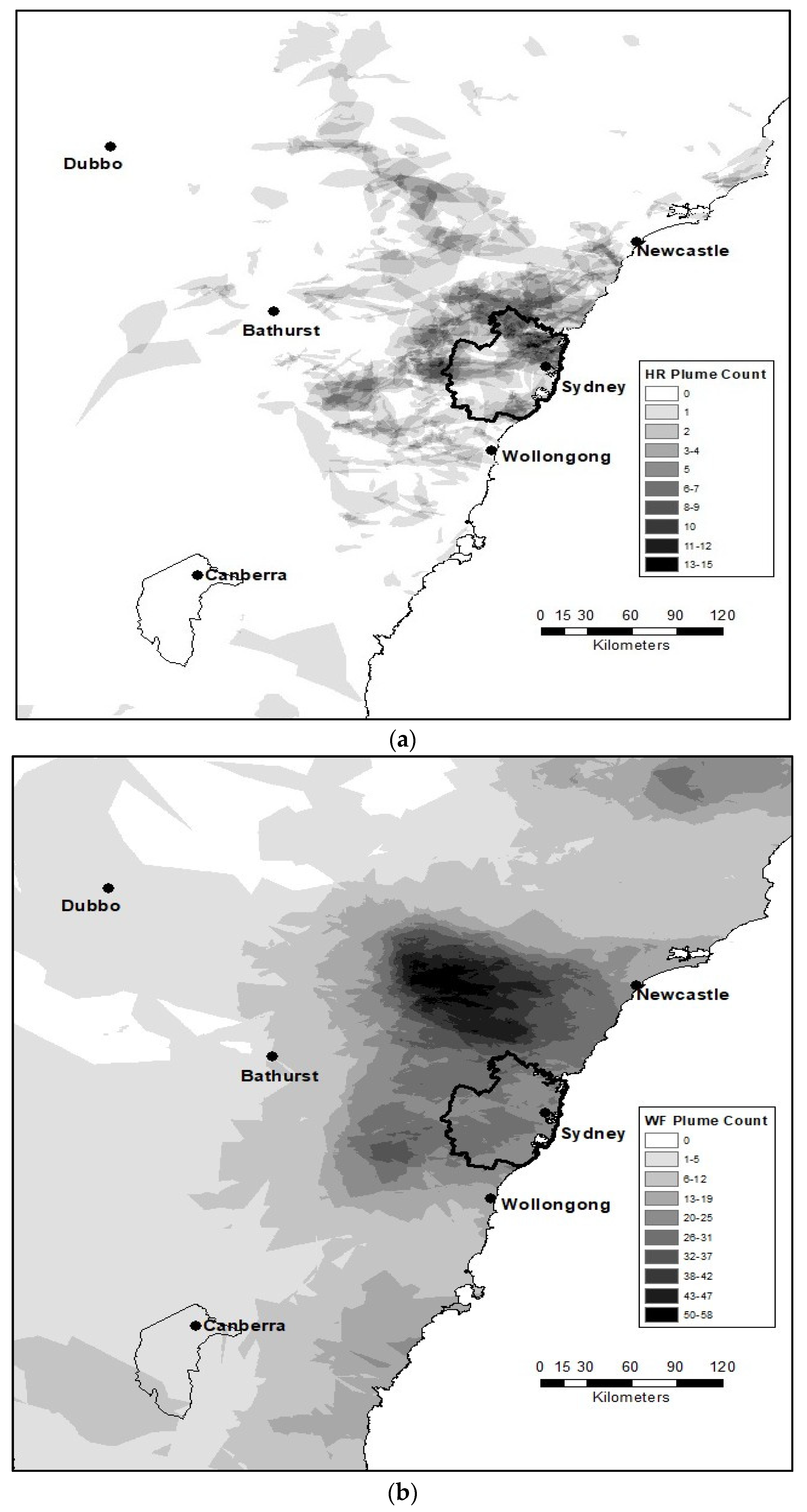
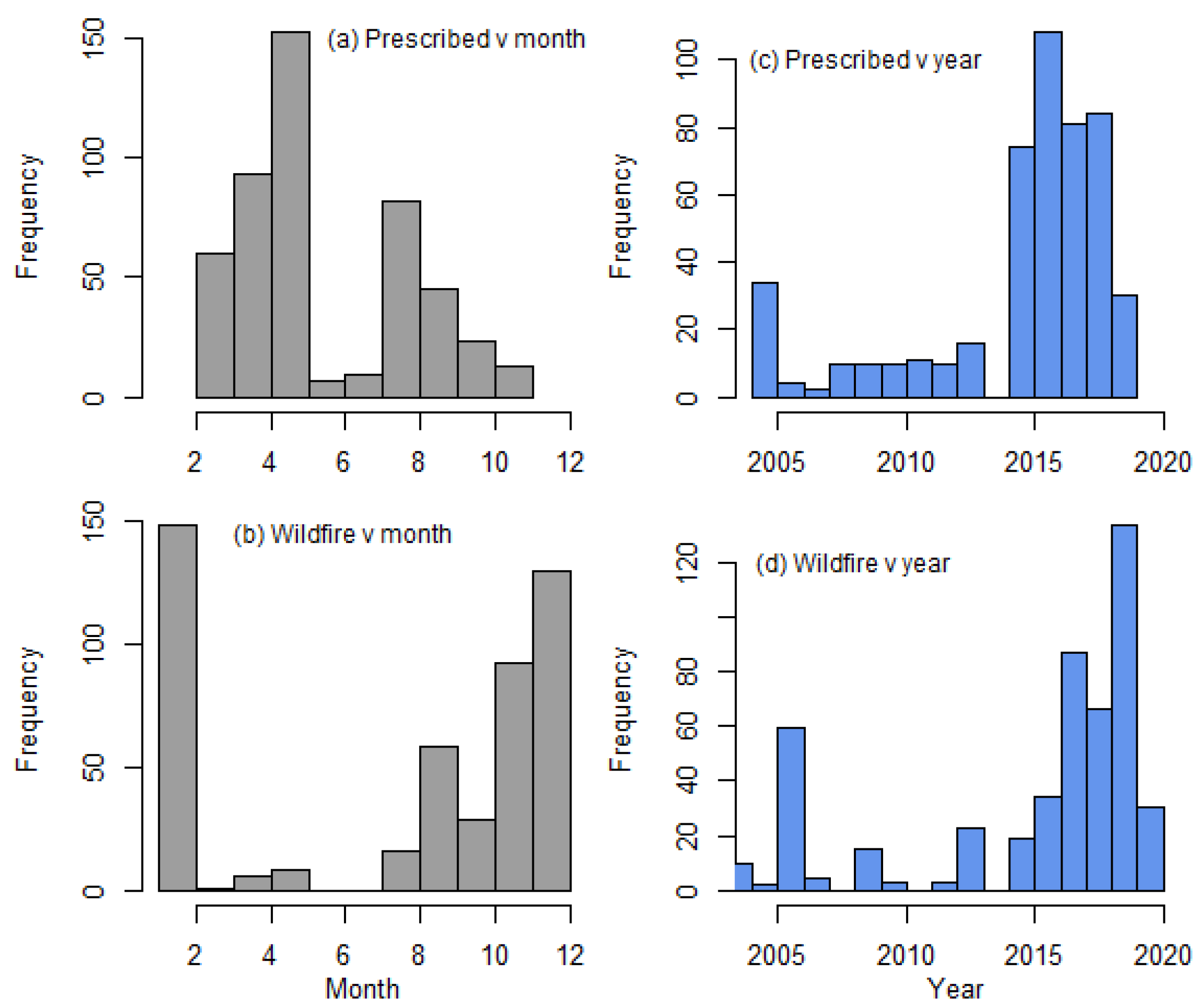
The median size of prescribed burn plumes was 6998 ha and that of wildfires was 10 times larger (69,540 ha). The map of plume frequencies shows that prescribed burn plumes tend to be concentrated on the northern and western edges of Greater Sydney (areas such as Berowra and the Nepean river), while the maximum number of plumes experienced was 15 (Figure 1a). In contrast, wildfire plume frequency was higher, with a maximum of 58 plumes, and concentrated further from Sydney (~100 km northwest in the Wollemi National Park, Figure 1b). When the 2019/20 wildfires were excluded, the wildfire map was similar, with the main hotspot still over the Wollemi National Park, and a maximum of 26 plumes. Prescribed fire plumes were most common in May but also occurred from March until November (Figure 2a). In contrast, wildfire plumes were most common in December and January and were rare in Autumn and winter months (March to August, Figure 2b). When 2019-20 bushfires were excluded from the wildfire plumes, January was the most common month. The spread across years was concentrated on recent years for both prescribed (median 2016, Figure 2c) and wildfires (median 2017, Figure 2d). A total of 34% of wildfire plumes were in the 2019/20 Black Summer season.
Wildfire plumes tended to occur over areas with low populations. Those with 1–3 wildfire plumes had a mean population density of 4.9 people per km2 though 79% of affected cells had zero population, while those with more than three plumes has a mean of 36 people and 71% had zero population. In contrast, cells with 1–3 prescribed burns had a mean population of 100 people and 71% had zero population, while those with more than three plumes has a mean of 189 people, and 62% with zero population.
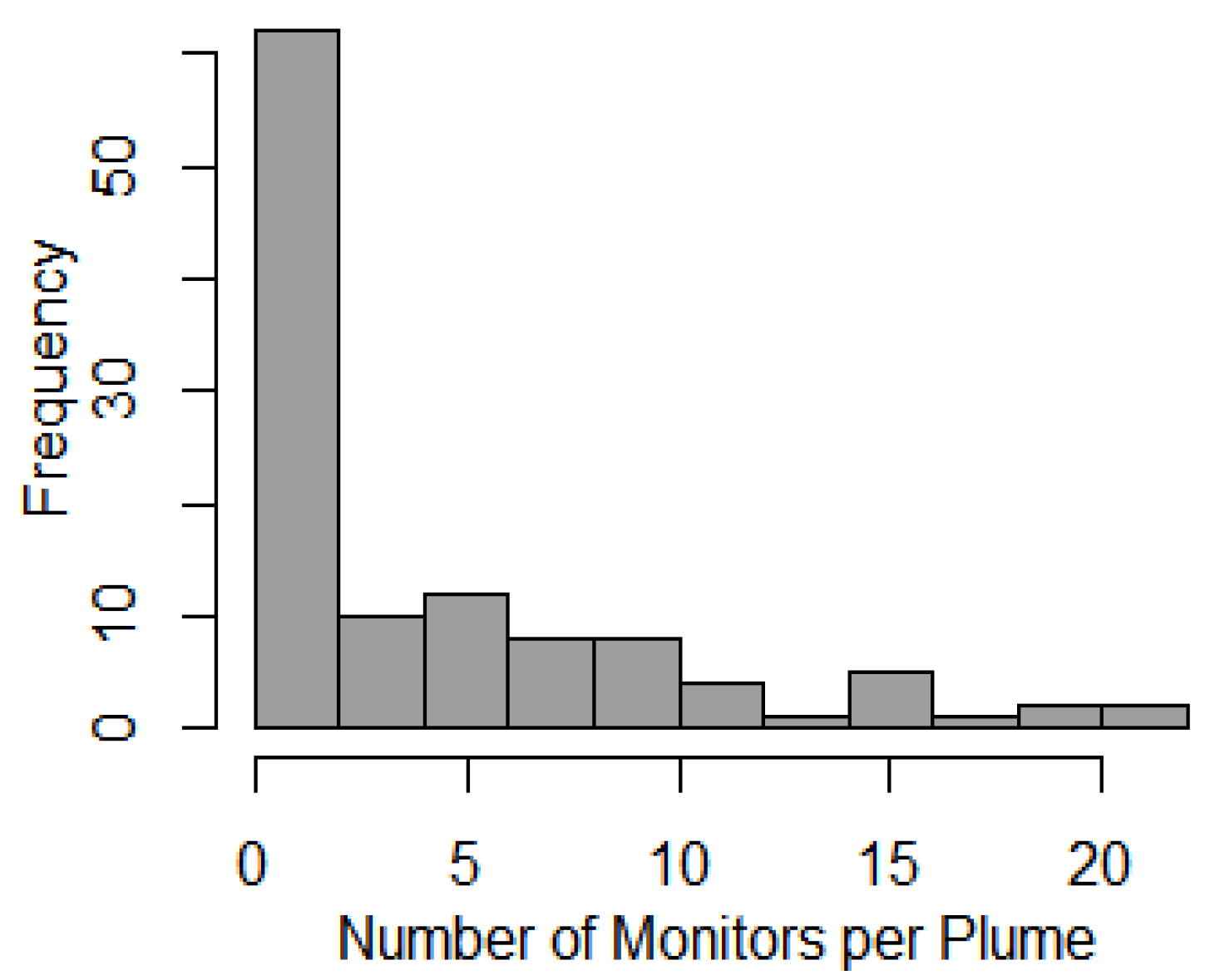
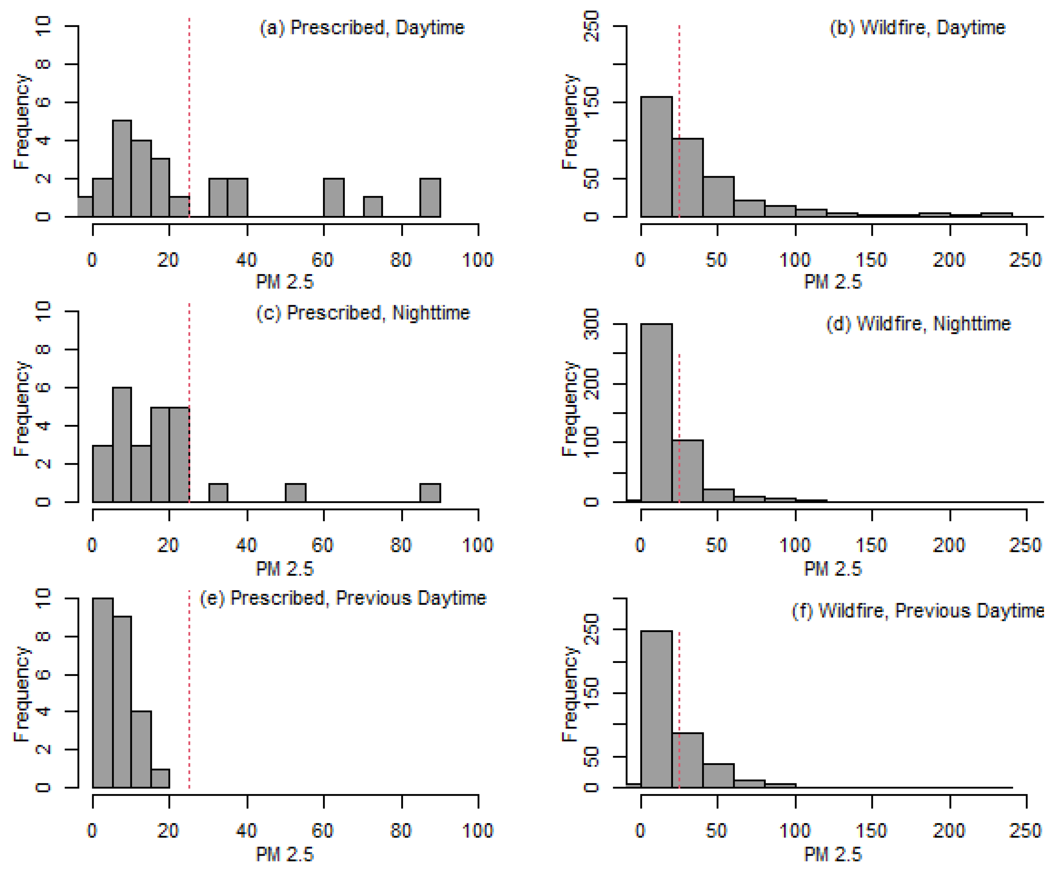
Only 115 of the plumes passed over an air quality monitor, comprising 22 prescribed and 93 wildfires (meaning 4.1% of mapped prescribed and 18.2% of wildfires passed over a monitor). Most of these plumes passed over only one or two monitors, but 15% of them passed over 10 or more (Figure 3). In total, there were 542 observations in the air quality sample (combinations of plumes and monitors), though due to interruptions in the PM2.5 record, there were only 395 valid daytime observations and 474 valid nighttime observations. Almost 71% of the observations were from the 2019-20 Black Summer bushfire season and only 5% (27) were from prescribed burns. For prescribed burns, the PM2.5 values for prescribed burns in the daytime period had a median value of 15.6 μgm−3 and a maximum of 89.9 μgm−3 with 33% of cases causing an exceedance (Figure 4a). For the night period, the distribution was similar (median 15.2 μgm−3, maximum 87.4 μgm−3), but only 11% caused an exceedance (Figure 4c). None of the previous daytime values were exceedances and the median value was lower at 5.8 μgm−3 (Figure 4e). For wildfires, there was a much larger range of PM2.5 values. In the daytime, the median value was 24.4 μgm−3 and the maximum of 370 μgm−3, with 48% exceedance (Figure 4b). For nighttime, the median and maximum were lower at 15.2 μgm−3 and 291 μgm−3, respectively, and 22% exceedance (Figure 4e). The previous daytime was lower, but much higher than the days previous to prescribed burns, with a median of 14.8 μgm−3 and a maximum of 238 μgm−3, with 27% exceedances (Figure 4f).
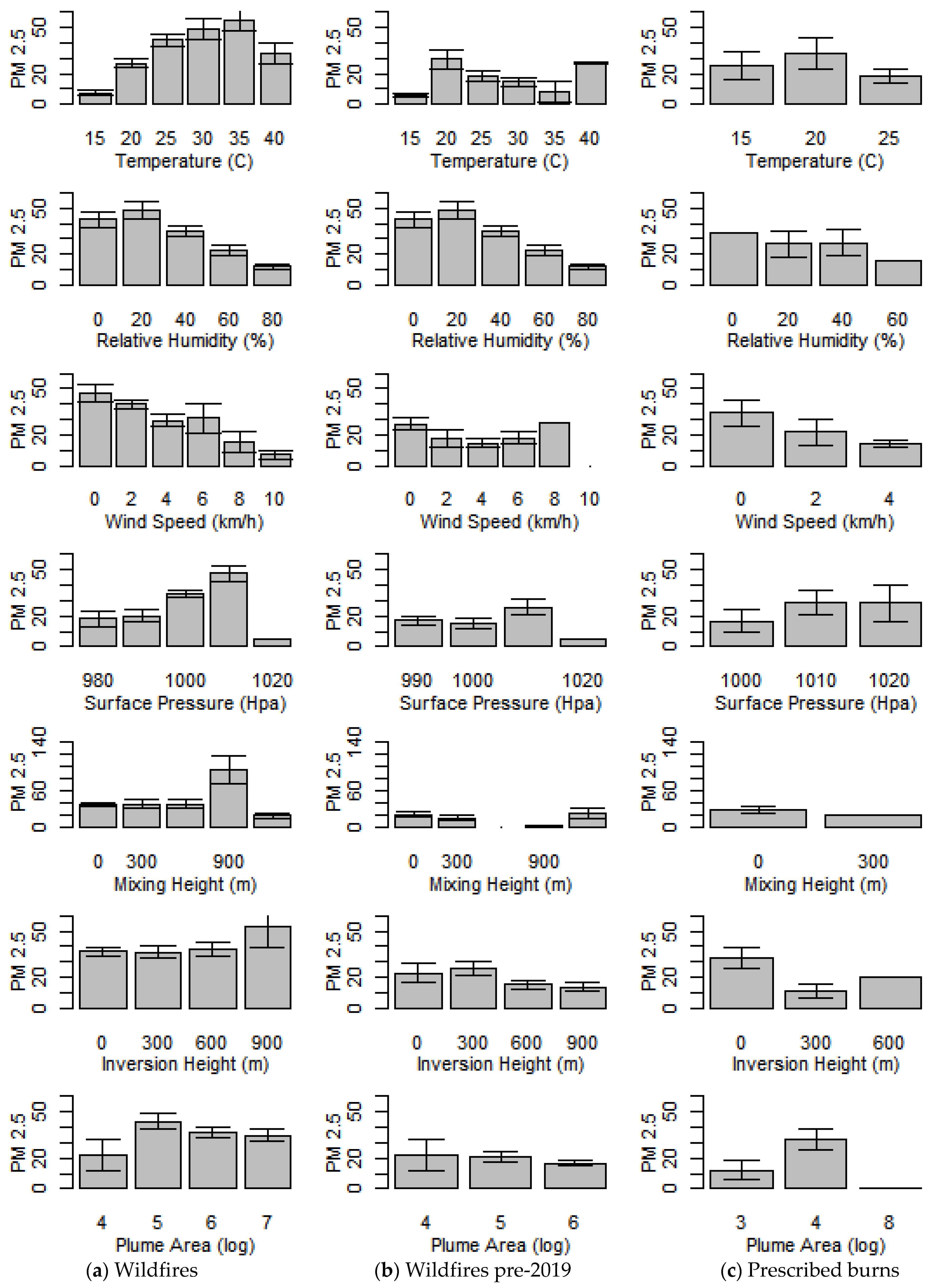
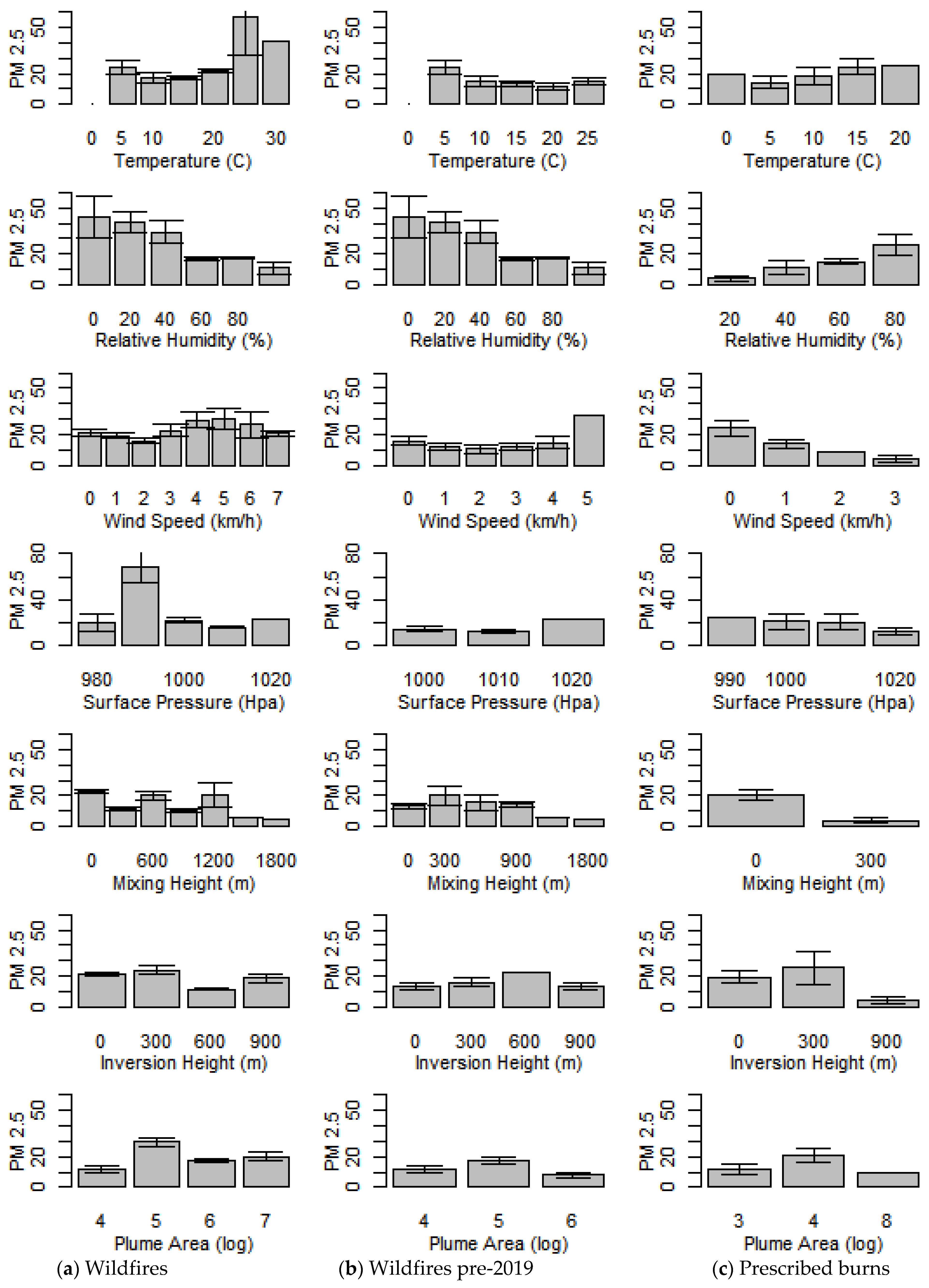
PM2.5 values underneath the plumes appeared to show relationships with several of the atmospheric predictors (Figure 5 and Figure 6). For daytime observations under wildfires, there was a positive relationship with temperature and surface pressure, a negative relationship with wind speed, relative humidity, and no relationship with mixing height, inversion height, or plume area (Figure 5a). When the 2019-20 fire season was excluded, the relationships were similar but not so obvious, with some indication of an opposite relationship with temperature (negative, Figure 5b). Prescribed burns showed the same relationships as wildfires with wind speed, relative humidity, and surface pressure, but no obvious relationship to the other predictors (Figure 5c). For nighttime observations, wildfires showed fewer relationships than they did for daytime observations, the only obvious ones being a negative relationship with relative humidity and mixing height (Figure 6a). Excluding the 2019-20 fire season did not reveal any different relationships (Figure 6b). Prescribed burns showed a positive relationship with relative humidity (opposite of wildfires and of prescribed burns in the daytime), a negative relationship with wind speed, mixing height, and inversion height (Figure 6c).
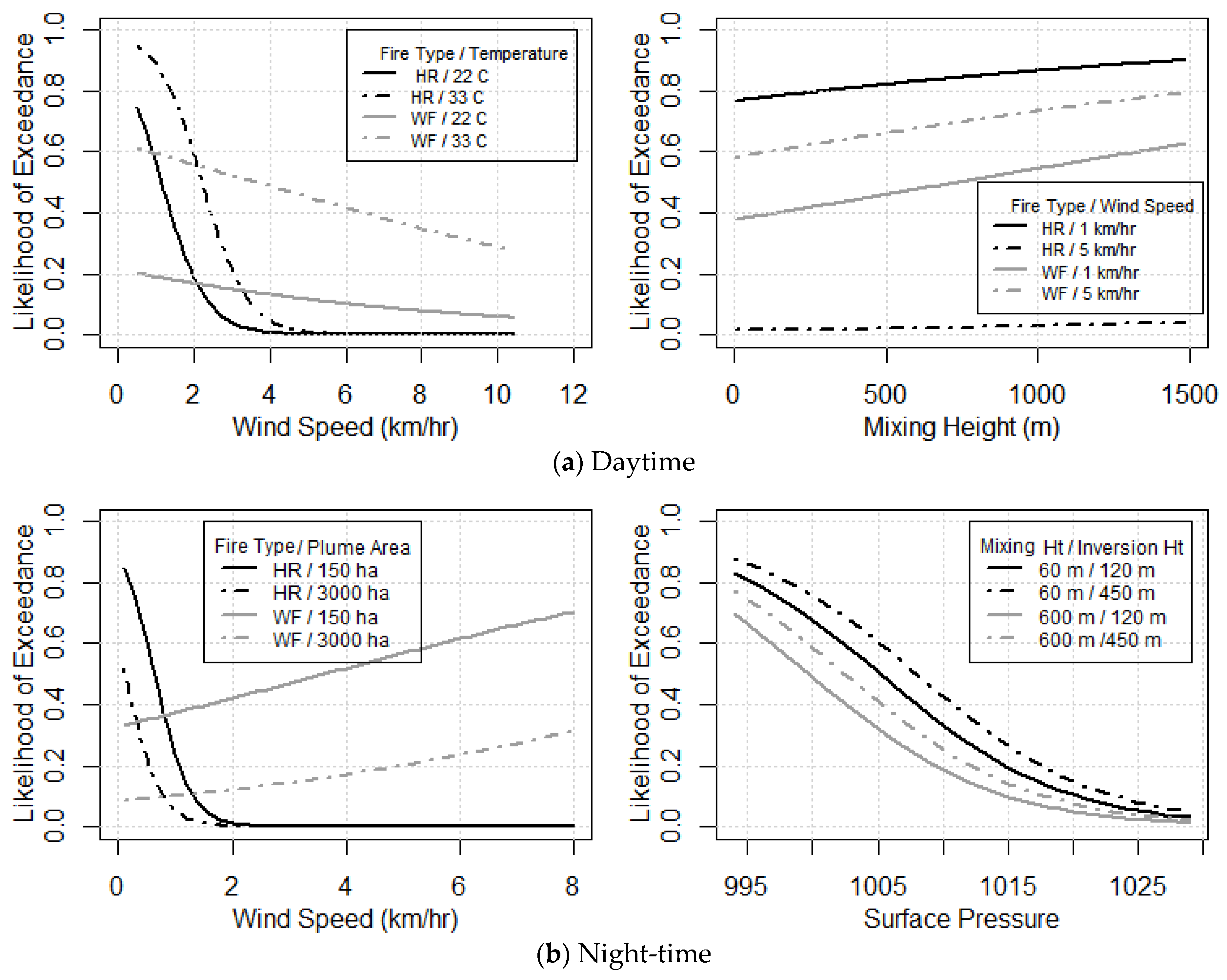
The binomial regression model for daytime poor air quality exceedances identified a negative effect of wind speed, positive effects of temperature and mixing height, and an interaction between wind speed and fire type, such that the wind speed effect was strong for prescribed burns and negligible for wildfires (Table 2, Figure 7a). For a prescribed burn, if the air is still (wind speed < 1 km/h), then an exceedance is almost certain, but the likelihood falls to near zero once wind speed exceeds 4 km/h. For wildfires, the likelihood of exceedance is lower and decreases more gradually with increasing wind speed. For both prescribed and wild fires, warmer temperatures increase the likelihood of exceedance (by about 0.04 per degree C). The mixing height effect was small for both prescribed and wildfires (likelihood increases by <0.1 per 1000 m increase in mixing height). The model captured only 10.8% of null deviance. The model without the 2019-20 wildfires was somewhat different and contained fewer terms. It identified a similar temperature effect as the full model, but also a positive effect of air pressure and negative effects of relative humidity.
The binomial model for nighttime poor air quality exceedances identified negative effects of air pressure, wind speed, mixing height, and plume area, and a positive effect of inversion height (Table 2, Figure 7b). As with daytime exceedances, there was a fire- type interaction with wind speed such that the negative relationship was much weaker in wildfires. The nighttime model captured 14.0% of null deviance. The model excluding 2019-20 wildfires was simpler but identified similar wind speed, mixing height, plume area, and fire type effects. However, air pressure was not present in the model.
4. Discussion
Smoke plumes are a common phenomenon in NSW: we observed an average of 100 per year in the zone 250 km around Sydney. The number of plumes per year increased over the study period. In both cases, the cause is probably the deepening drought from 2015 which culminated in the Black Summer season of 2019-20, but which also allowed more opportunities for prescribed burning We only detected plumes for 20% of known fires. Most of this under-reporting is probably due to the size of the fires. A total of 65% of prescribed burns and 70% of wildfires in the fire history data were smaller than 25 ha (one MODIS pixel), which means their plumes are probably also small and hard to detect on the imagery. It is likely that these have only localized smoke plumes and so do not affect the major towns, so the consequences of failing to detect them may be minor. There is also a problem of clouds obscuring the plumes. We could not obtain a robust estimate of how many plumes were missed for this reason. In general, cloud cover was usually low on days with high fire activity, but we did encounter several cases where clouds occurred on days we expected to see a plume (due to large fires burning on those days).
The seasonal patterns of plumes (wildfires in summer and prescribed fires in spring and autumn) confirm to well-known patterns. Wildfire plumes occur when the weather is hot and dry, and prescribed burns avoid those times and also avoid Winter when fires usually do not spread. Wildfire plumes tended to occur in the forested National Parks away from Sydney while prescribed fire plumes were closer to Sydney. This pattern is reflected in the population density figures under the plumes. Even though the majority of the areas under plumes had zero population, the mean population density under prescribed burn plumes was more than 10 times that for wildfire plumes. This difference is almost certainly because many of the prescribed burns are placed in the wildland urban interface, close to houses [15].
Only 4.1% of prescribed burns and 18.2% of wildfires plumes passed over an air quality monitor. The discrepancy between fire types is, in part, because wildfire plumes are, on average, 10 times larger than prescribed burn plumes. The low rate of overlap with monitors is also because most plumes occurred over forested areas (especially wildfire plumes), whereas air quality monitors are mostly situated in urban centres. Monitors are situated in population centres as their primary role is to detect anthropogenic pollution sources. Currently, the NSW Department of Planning and Environment maintains 36 compliance standard monitors, 27 of which are in the greater Sydney region, though there are 58 monitors spread more broadly around the state that are not compliant with the National Environmental (Ambient Air Quality) Measure (NEPM) [27]. The low rate of overlap suggests that air quality monitors are not well placed for detecting fire smoke. This is a problem for studies such as ours that try to understand the relationship between fires and human exposure because the samples are small. However, in terms of optimizing the network, there Is a balance between monitoring places with high levels of smoke (forests) and the bulk of the people who may be affected by smoke and other pollutants (cities). This is not an easy problem to solve.
Most wildfire plumes remain aloft: only 38% of wildfire and 33% of prescribed fire plumes caused an exceedance. This is encouraging from the point of view that fires and their plumes do not necessarily impact people. However, it does complicate the task of predicting smoke impact. An evaluation of the US NOAA smoke forecasting system that partially relies on the HMS plume mapping method we applied, found an average of only 10% congruence between forecast and actual particulate concentrations [21]. Plumes remaining aloft are probably a contributor to this poor performance, a point conceded by [30]. There have been more than 100 studies relating air quality to satellite-derived metrics (particularly Aerosol Optical Depth, AOD), and most of these report explanatory power (r2) above 0.7 [24]. AOD measures the extinction of light as it passes through the atmosphere but provides no information about where in the column the opaque air is. Clearly, our results suggest that in many cases of smoke, AOD cannot easily be equated to surface air quality. Nor are physically derived atmospheric dispersal models good at predicting ground-level smoke concentrations, with r2 typically around 0.4 [19,20,31]. It is not clear the extent to which these physical models are able to resolve the question of whether plumes remain aloft, but it is likely that it remains a challenge.
Our study revealed several important meteorological controls on smoke impact. Probably the most important is that prescribed burn plumes were much more likely to cause an exceedance if the wind speed was less than 4 kmhr−1. Wind speed is the only factor that showed a strong difference between prescribed burns and wildfires. The effect is in agreement with many other studies that find still air to be a particular risk factor for prescribed burn smoke impact [9,32,33] and for poor air quality generally [34,35,36]. In theory, it would be possible for burn practitioners to avoid low wind speeds, but this is difficult in practice because these are ideal for reducing the risk of fire escape, and burn prescriptions discourage burning in strong winds for this reason [37]. Low wind speed was much less of a risk factor for wildfires. This is probably because, under those conditions, the smoke plume is less likely to reach an air quality monitor (predominantly in the city of Sydney) than from a prescribed fire, because wildfires tend to occur further from the wildland-urban interface [15]. For wildfires, wind speed itself is not the only risk factor related to wind. Conditions that trap air in the Sydney basin are important, which principally occurs when there are westerly winds, countered by an easterly sea breeze that prevents air escaping to the ocean [38,39].
The temperature has a complex relationship with smoke. In our models, there was a positive effect on the risk of exceedance during the day, but not at night. Other studies find higher risk either in low temperatures [9,32] or at both low and high temperatures (u-shaped relationship) [38]. It is likely that low temperatures are a feature of still, stable air in the winter (prescribed burning season), which contributes to smoke descending to the ground, but high temperatures increase fire activity and hence overall smoke production.
Our study gave conflicting evidence about atmospheric stability. The daytime model suggested the risk of exceedance increases with mixing height, while the night-time model had a negative effect of mixing height combined with a negative effect of air pressure and a positive effect of inversion height, though all of them were weak effects. Of these, the negative daytime mixing height and the night-time inversion height effects correspond with the expectation that a low inversion and low mixing height should prevent smoke from rising or moving away. The air pressure effect is hard to explain because it is generally considered that high pressure which brings stable, still air is bad for air quality [34,39]. As with the effects of temperature, there might be a tension between the atmospheric controls on smoke settling and those on fire activity that produces the smoke. For example, the C-Haines [40] measure of mid-level atmospheric instability has been found to be positively related to particulate concentrations in Sydney considering all days with fire activity [36], but negatively related to concentrations in the vicinity of prescribed burns in the same region [9]. In other words, it is possible that stable air dampens the production of smoke, but concentrates it near the ground.
5. Conclusions
Our study has found an increase in the number of plumes from both prescribed and wildfires since 2015, probably associated with drought conditions. Prescribed burn plumes tended to occur over more populated areas than wildfires. A small minority of plumes passed over a monitor so the current network is not optimized for detecting smoke. A minority of plumes caused a detectable increase in PM2.5, whether prescribed or wildfire plumes in day or night-time, so most plumes remained aloft (did not reach the surface). Various aspects of weather influenced whether a plume caused an exceedance, and, in wind speeds below 1 kmhr−1, exceedance was almost certain in prescribed burn plumes that passed over an AQ monitor.
The phenomena identified in this study will be useful for planning prescribed burning, preparing warnings, and improving our ability to predict smoke impacts. However, in terms of improving the prediction of smoke impacts from specific fires, our model’s performance is similar to that reported for physical models of PM2.5 [19,20,31], and other empirical models, such as predicting PM2.5 concentrations at air quality monitors as a consequence of individual fires or on days when fires occurred [26,36,38]. Accurate prediction of PM2.5 concentrations remains a complex and elusive goal. There is a need to build multiple lines of evidence, including further empirical research on patterns of smoke production, transport, and exposure, in conjunction with refinements in physical models (which the empirical research can help to validate).
Author Contributions
Conceptualization, O.F.P.; methodology, O.F.P.; formal analysis, O.F.P. and S.R.; data creation, S.R. and S.S.; writing—original draft preparation, S.R. and O.F.P.; writing—review and editing, O.F.P., S.R. and S.S. All authors have read and agreed to the published version of the manuscript.
Funding
This research was funded by the NSW Department of Planning and Environment through the Bushfire Risk Management Research Hub.
Institutional Review Board Statement
Not applicable.
Informed Consent Statement
Not applicable.
Data Availability Statement
The data forming the analysis in this paper are available from Figshare (https://figshare.com/articles/dataset/Price_2023_Fire_data/22151804).
Acknowledgments
We would like to thank Grant J. Williamson for providing MODIS plumes and staff from the Department of Planning and Environment who supplied the air quality data. Simin Rahmani undertook this study as part of her MSc program at the University of Wollongong.
Conflicts of Interest
The authors declare no conflict of interest.
References
- Borchers Arriagada, N.; Palmer, A.J.; Bowman, D.M.J.S.; Morgan, G.G.; Jalaludin, B.B.; Johnston, F.H. Unprecedented smoke-related health burden associated with the 2019–20 bushfires in eastern Australia. Med. J. Aust. 2020, 213, 282. [Google Scholar] [CrossRef] [PubMed]
- Johnston, F.H.; Henderson, S.B.; Chen, Y.; Randerson, J.T.; Marlier, M.; DeFries, R.S.; Kinney, P.; Bowman, D.; Brauer, M. Estimated global mortality attributable to smoke from landscape fires. Environ. Health Perspect. 2012, 120, 695–701. [Google Scholar] [CrossRef] [PubMed] [Green Version]
- Williams, A.P.; Abatzoglou, J.T.; Gershunov, A.; Guzman-Morales, J.; Bishop, D.A.; Balch, J.K.; Lettenmaier, D.P. Observed impacts of anthropogenic climate change on wildfire in California. Earths Future 2019, 7, 892–910. [Google Scholar] [CrossRef] [Green Version]
- Canadell, J.G.; Meyer, C.P.; Cook, G.D.; Dowdy, A.; Briggs, P.R.; Knauer, J.; Pepler, A.; Haverd, V. Multi-decadal increase of forest burned area in Australia is linked to climate change. Nat. Commun. 2021, 12, 6921. [Google Scholar] [CrossRef] [PubMed]
- Liu, Y.Q.; Liu, Y.; Fu, O.S.; Yang, C.E.; Dong, X.Y.; Tian, H.Q.; Tao, B.; Yang, J.; Wang, Y.H.; Zou, Y.F.; et al. Projection of future wildfire emissions in western USA under climate change: Contributions from changes in wildfire, fuel loading and fuel moisture. Int. J. Wildland Fire 2022, 31, 1–13. [Google Scholar] [CrossRef]
- Williamson, G.; Bowman, D.; Price, O.; Henderson, S.; Johnston, F. A transdisciplinary approach to understanding the health effects of wildfire and prescribed smoke. Environ. Res. Lett. 2016, 11, 125009. [Google Scholar] [CrossRef]
- Fernandes, P.M.; Botelho, H.S. A review of prescribed burning effectiveness in fire hazard reduction. Int. J. Wildland Fire 2003, 12, 117–128. [Google Scholar] [CrossRef] [Green Version]
- Broome, R.A.; Johnstone, F.H.; Horsley, J.; Morgan, G.G. A rapid assessment of the impact of hazard reduction burning around Sydney, May 2016. Med. J. Aust. 2016, 205, 407–408. [Google Scholar] [CrossRef]
- Price, O.F.; Forehead, H. Smoke patterns around prescribed fires in Australian eucalypt forests, as measured by low-cost particulate monitors. Atmosphere 2021, 12, 1389. [Google Scholar] [CrossRef]
- Navarro, K.M.; Schweizer, D.; Balmes, J.R.; Cisneros, R. A Review of Community Smoke Exposure from Wildfire Compared to Prescribed Fire in the United States. Atmosphere 2018, 9, 185. [Google Scholar] [CrossRef] [Green Version]
- Afrin, S.; Garcia-Menendez, F. The Influence of Prescribed Fire on Fine Particulate Matter Pollution in the Southeastern United States. Geophys. Res. Lett. 2020, 47, e2020GL088988. [Google Scholar] [CrossRef]
- Afrin, S.; Garcia-Menendez, F. Potential impacts of prescribed fire smoke on public health and socially vulnerable populations in a Southeastern US state. Sci. Total Environ. 2021, 794, 148712. [Google Scholar] [CrossRef]
- Price, O.F.; Pausas, J.C.; Govender, N.; Flannigan, M.; Fernandes, P.M.; Brooks, M.L.; Bird, R.B. Global patterns in fire leverage: The response of annual area burnt to previous fire. Int. J. Wildland Fire 2015, 24, 297–306. [Google Scholar] [CrossRef] [Green Version]
- Bradstock, R.A.; Boer, M.M.; Cary, G.J.; Price, O.F.; Williams, R.J.; Barrett, D.; Cook, G.; Gill, A.M.; Hutley, L.B.; Keith, H.; et al. Modelling the potential for prescribed burning to mitigate emissions from fire-prone, Australian ecosystems. Int. J. Wildland Fire 2012, 21, 629–639. [Google Scholar] [CrossRef]
- Price, O.F.; Bradstock, R.A. The spatial domain of wildfire risk and response in the Wildland Urban Interface in Sydney, Australia. Nat. Hazards Earth Syst. Sci. 2013, 13, 3385–3393. [Google Scholar] [CrossRef] [Green Version]
- Crawford, J.; Chambers, S.; Cohen, D.D.; Williams, A.; Griffiths, A.; Stelcer, E.; Dyer, L. Impact of meteorology on fine aerosols at Lucas Heights, Australia. Atmos. Environ. 2016, 145, 135–146. [Google Scholar] [CrossRef]
- Pearce, J.L.; Rathbun, S.; Achtemeier, G.; Naeher, L.P. Effect of distance, meteorology, and burn attributes on ground-level particulate matter emissions from prescribed fires. Atmos. Environ. 2012, 56, 203–211. [Google Scholar] [CrossRef]
- Riebau, A.R.; Fox, D. The new smoke management. Int. J. Wildland Fire 2001, 10, 415–427. [Google Scholar] [CrossRef]
- Yao, J.; Brauer, M.; Henderson, S.B. Evaluation of a Wildfire Smoke Forecasting System as a Tool for Public Health Protection. Environ. Health Perspect. 2013, 121, 1142–1147. [Google Scholar] [CrossRef]
- Price, O.F.; Horsey, B.; Jiang, N. Local and regional smoke impacts from prescribed fires. Nat. Hazards Earth Syst. Sci. 2016, 16, 2247–2257. [Google Scholar] [CrossRef] [Green Version]
- Rolph, G.D.; Draxler, R.R.; Stein, A.F.; Taylor, A.; Ruminski, M.G.; Kondragunta, S.; Zeng, J.; Huang, H.-C.; Manikin, G.; McQueen, J.T.; et al. Description and verification of the NOAA smoke forecasting system: The 2007 fire season. Weather Forecast. 2009, 24, 361–378. [Google Scholar] [CrossRef]
- Williamson, G.J.; Price, O.F.; Henderson, S.B.; Bowman, D.M.J.S. Satellite-based comparison of fire intensity and smoke emissions from prescribed and wildfires in south-eastern Australia. Int. J. Wildland Fire 2013, 22, 121–129. [Google Scholar] [CrossRef]
- Paul, N.; Yao, J.Y.; McLean, K.E.; Stieb, D.M.; Henderson, S.B. The Canadian optimized statistical smoke exposure model (CanOSSEM): A machine learning approach to estimate national daily fine particulate matter (PM2.5) exposure. Sci. Total Environ. 2022, 850, 157956. [Google Scholar] [CrossRef] [PubMed]
- Chu, Y.Y.; Liu, Y.S.; Li, X.Y.; Liu, Z.Y.; Lu, H.S.; Lu, Y.A.; Mao, Z.F.; Chen, X.; Li, N.; Ren, M.; et al. A review on predicting ground pm2.5 concentration using satellite aerosol optical depth. Atmosphere 2016, 7, 129. [Google Scholar] [CrossRef] [Green Version]
- Williamson, G.J.; Lucani, C. AQVx-an interactive visual display system for air pollution and public health. Front. Public Health 2020, 8, 85. [Google Scholar] [CrossRef]
- Yao, J.Y.; Henderson, S.B. An empirical model to estimate daily forest fire smoke exposure over a large geographic area using air quality, meteorological, and remote sensing data. J. Expo. Sci. Environ. Epidemiol. 2014, 24, 328–335. [Google Scholar] [CrossRef] [Green Version]
- Anon. New South Wales Annual Compliance Report 2020, National Environment Protection (Ambient Air Quality) Measure; Office of Environment and Heritage: Sydney, NSW, Australia, 2021; p. 108. [Google Scholar]
- Seidel, D.J.; Ao, C.O.; Li, K. Estimating climatological planetary boundary layer heights from radiosonde observations: Comparison of methods and uncertainty analysis. J. Geophys. Res.-Atmos. 2010, 115, D16113. [Google Scholar] [CrossRef] [Green Version]
- Price, O.F.; Purdam, P.J.; Bowman, D.M.J.S.; Williamson, G. Comparing the height and area of wild and prescribed fire smoke particle plumes in southeast Australia using weather radar. Int. J. Wildland Fire 2018, 27, 525–537. [Google Scholar] [CrossRef]
- Kaulfus, A.S.; Nair, U.; Jaffe, D.; Christopher, S.A.; Goodrick, S. Biomass burning smoke climatology of the United States: Implications for particulate matter air quality. Environ. Sci. Technol. 2017, 51, 11731–11741. [Google Scholar] [CrossRef]
- Guerette, E.A.; Chang, L.T.C.; Cope, M.E.; Duc, H.N.; Emmerson, K.M.; Monk, K.; Rayner, P.J.; Scorgie, Y.; Silver, J.D.; Simmons, J.; et al. Evaluation of regional air quality models over Sydney, Australia: Part 2, comparison of PM2.5 and ozone. Atmosphere 2020, 11, 233. [Google Scholar] [CrossRef]
- Di Virgilio, D.; Hart, M.A.; Jiang, N. Meteorological controls on atmospheric particulate pollution during hazard reduction burns. Atmos. Chem. Phys. 2018, 18, 6585–6599. [Google Scholar] [CrossRef] [Green Version]
- Miller, C.; O’Neill, S.; Rorig, M.; Alvarado, E. Air-quality challenges of prescribed fire in the complex terrain and wildland urban interface surrounding bend, Oregon. Atmosphere 2019, 10, 515. [Google Scholar] [CrossRef] [Green Version]
- Hart, M.; De Dear, R.; Hyde, R. A synoptic climatology of tropospheric ozone episodes in Sydney, Australia. Int. J. Climatol. 2006, 26, 1635–1649. [Google Scholar] [CrossRef]
- Crawford, J.; Chambers, S.; Cohen, D.; Williams, A.; Griffiths, A.; Stelcer, E. Assessing the impact of atmospheric stability on locally and remotely sourced aerosols at Richmond, Australia, using Radon-222. Atmos. Environ. 2016, 127, 107–117. [Google Scholar] [CrossRef]
- Price, O.F.; Williamson, G.J.; Henderson, S.B.; Johnston, F.; Bowman, D.J.M.S. The relationship between landscape fire activity from Modis Hotspots and particulate pollution levels in Australian cities. PLoS ONE 2012, 7, e47327. [Google Scholar] [CrossRef] [PubMed] [Green Version]
- Clarke, H.; Tran, B.; Boer, M.; Price, O.; Kenny, B.; Bradstock, R. Climate change effects on the frequency, seasonality and interannual variability of suitable prescribed burning weather conditions in south-eastern Australia. Agric. For. Meteorol. 2019, 271, 148–157. [Google Scholar] [CrossRef]
- Storey, M.A.; Price, O.F. Prediction of air quality in Sydney, Australia as a function of forest fire load and weather using Bayesian statistics. PLoS ONE 2022, 17, e0272774. [Google Scholar] [CrossRef]
- Jiang, N.B.; Scorgie, Y.; Hart, M.; Riley, M.L.; Crawford, J.; Beggs, P.J.; Edwards, G.C.; Chang, L.S.; Salter, D.; Virgilio, G.D. Visualising the relationships between synoptic circulation type and air quality in Sydney, a subtropical coastal-basin environment. Int. J. Climatol. 2017, 37, 1211–1228. [Google Scholar] [CrossRef]
- Mills, G.; McCaw, L. Atmospheric Stability Environments and Fire Weather in Australia—Extending the Haines Index; Centre for Australian Weather and Climate Research: Melbourne, VIC, Australia, 2010; p. 151. [Google Scholar]
Figure 1.
Map of smoke plume frequency for 2002–2020 for (a) prescribed burns and (b) wildfires. The Greater Sydney area is outlined in black. High density in b is centered on Wollemi National Park. Notice the different scales for the shading.
Figure 1.
Map of smoke plume frequency for 2002–2020 for (a) prescribed burns and (b) wildfires. The Greater Sydney area is outlined in black. High density in b is centered on Wollemi National Park. Notice the different scales for the shading.

Figure 2.
Frequency distribution of plumes for prescribed and wildfires by month (a,b) and year (c,d).
Figure 2.
Frequency distribution of plumes for prescribed and wildfires by month (a,b) and year (c,d).

Figure 3.
Histogram of the number of monitors each plume passed over (excluding those over no monitor).
Figure 3.
Histogram of the number of monitors each plume passed over (excluding those over no monitor).

Figure 4.
Distribution of PM2.5 values for the plumes that passed over an air-quality monitor: For prescribed burns (a) during the day of the overpass, (c) the following night, and (e) the previous daytime for comparison. (b,d,f) are the same for wildfires. The vertical dotted line is the exceedance level (25 μgm−3).

Figure 5.
Relationship between daytime PM2.5 values and predictor variables for (a) Wildfire plumes, (b) Wildfire plumes excluding the 2019-20 season, and (c) Prescribed burn plumes.
Figure 5.
Relationship between daytime PM2.5 values and predictor variables for (a) Wildfire plumes, (b) Wildfire plumes excluding the 2019-20 season, and (c) Prescribed burn plumes.

Figure 6.
Relationship between night-time PM2.5 values and predictor variables for (a) Wildfire plumes, (b) Wildfire plumes excluding the 2019-20 season, and (c) Prescribed burn plumes.
Figure 6.
Relationship between night-time PM2.5 values and predictor variables for (a) Wildfire plumes, (b) Wildfire plumes excluding the 2019-20 season, and (c) Prescribed burn plumes.

Figure 7.
Binomial model relationships for (a) daytime and (b) night-time poor air quality exceedances.
Figure 7.
Binomial model relationships for (a) daytime and (b) night-time poor air quality exceedances.


Table 1.
Variables used in the statistical analysis.
| Variable Name | Description | Missing Values |
|---|---|---|
| Dependent Variables | ||
| Day exceedance | Mean PM2.5 for 12:30–3:30 p.m. is >25 μgm−3 and PM2.5 > same period on previous day. | 173 |
| Night exceedance | Mean PM2.5 for 1:30–4:30 a.m. is >18 μgm−3 and PM2.5 > same period on previous night. | 83 |
| Predictor Variables | ||
| Log (Plume Area) | Natural Log of the size of the mapped plume (in ha) | 0 |
| Fire type | Whether a wildfire (WF) or prescribed fire (PB) | 0 |
| Wind Speed | At the closest BOM automatic weather station at the time of maximum plume (Km/h) | 25 |
| Temperature | Temperature at the weather station (C) | 25 |
| Relative Humidity | Relative Humidity at the weather station (%) | 26 |
| Surface Pressure | Pressure at Sydney airport at 06:00 from upper atmospheric data (Hpa) | 19 |
| Mixing Height | Height above the ground at which the potential temperature is equal to the surface potential temperature. | 19 |
| Inversion Height | Height above ground at which temperature stops increasing with height, calculated from upper atmospheric data (m). | 19 |
Table 2.
Binomial regression models for daytime and nighttime observations of poor air quality exceedance. Each model was derived by fitting all predictors and testing the interaction with Fire Type for each selected variable. The table also shows the model for the subset of the data excluding the 2019-20 wildfires. An asterisk (*) indicates an interaction term.
| Variable | Estimate | Std. Error | z Value | Pr (>|z|) |
|---|---|---|---|---|
| Daytime Model (n = 350) | 10.8% of D | |||
| (Intercept) | −0.924 | 1.424 | −0.649 | 0.516 |
| Wind Speed | −1.687 | 0.845 | −1.997 | 0.046 |
| Temperature | 0.141 | 0.025 | 5.698 | 0.000 |
| Mixing Height | 0.00068 | 0.0003 | 2.064 | 0.039 |
| FireType Wildfire | −3.23 | 1.386 | −2.331 | 0.020 |
| Wind Speed * Fire Type: Wildfire | 1.543 | 0.849 | 1.818 | 0.069 |
| Day Excluding 2019 (n = 73) | 17.1% of D | |||
| (Intercept) | −185.70 | 68.42 | −2.714 | 0.007 |
| Air pressure | 0.179 | 0.066 | 2.722 | 0.006 |
| Temperature | 0.132 | 0.078 | 1.695 | 0.090 |
| Relative Humidity | −0.035 | 0.027 | −1.275 | 0.202 |
| Nighttime Model (n = 429) | 14.0% of D | |||
| (Intercept) | 150.60 | 28.05 | 5.370 | 0.000 |
| Wind Speed | −3.194 | 1.397 | −2.286 | 0.022 |
| FireType Wildfire | −2.755 | 1.185 | −2.326 | 0.020 |
| Air Pressure | −0.144 | 0.028 | −5.233 | 0.000 |
| Mixing Height | −0.001 | 0.000 | −3.088 | 0.002 |
| Inversion Height | 0.001 | 0.000 | 2.454 | 0.014 |
| Log (plume area) | −0.550 | 0.191 | −2.880 | 0.004 |
| Wind Speed:FireType Wildfire | 3.393 | 1.403 | 2.419 | 0.016 |
| Night Excluding 2019 (n = 76) | 15.0% of D | |||
| (Intercept) | 7.705 | 3.188 | 2.417 | 0.016 |
| Wind Speed | −2.881 | 1.445 | −1.993 | 0.046 |
| FireType Wildfire | −1.872 | 1.219 | −1.536 | 0.125 |
| Mixing Height | −0.002 | 0.001 | −1.721 | 0.085 |
| Log (plume area) | −1.335 | 0.584 | −2.285 | 0.022 |
| Wind Speed:FireType Wildfire | 3.344 | 1.513 | 2.210 | 0.027 |
Disclaimer/Publisher’s Note: The statements, opinions and data contained in all publications are solely those of the individual author(s) and contributor(s) and not of MDPI and/or the editor(s). MDPI and/or the editor(s) disclaim responsibility for any injury to people or property resulting from any ideas, methods, instructions or products referred to in the content. |
© 2023 by the authors. Licensee MDPI, Basel, Switzerland. This article is an open access article distributed under the terms and conditions of the Creative Commons Attribution (CC BY) license (https://creativecommons.org/licenses/by/4.0/).
Share and Cite
MDPI and ACS Style
Price, O.F.; Rahmani, S.; Samson, S. Particulate Levels Underneath Landscape Fire Smoke Plumes in the Sydney Region of Australia. Fire 2023, 6, 86. https://doi.org/10.3390/fire6030086
AMA Style
Price OF, Rahmani S, Samson S. Particulate Levels Underneath Landscape Fire Smoke Plumes in the Sydney Region of Australia. Fire. 2023; 6(3):86. https://doi.org/10.3390/fire6030086
Chicago/Turabian StylePrice, Owen F., Simin Rahmani, and Stephanie Samson. 2023. "Particulate Levels Underneath Landscape Fire Smoke Plumes in the Sydney Region of Australia" Fire 6, no. 3: 86. https://doi.org/10.3390/fire6030086