Quality of Experience (QoE)-Aware Fast Coding Unit Size Selection for HEVC Intra-Prediction


1
Centre for Vision Speech and Signal Processing, University of Surrey, Guildford GU2 7XH, UK
2
Cardiff School of Technologies, Cardiff Metropolitan University, Cardiff CF5 2YB, UK
*
Author to whom correspondence should be addressed.
Future Internet 2019, 11(8), 175; https://doi.org/10.3390/fi11080175
Submission received: 27 June 2019
/
Revised: 1 August 2019
/
Accepted: 7 August 2019
/
Published: 11 August 2019
(This article belongs to the Special Issue Multimedia Quality of Experience (QoE): Current Status and Future Direction)
Abstract
:The exorbitant increase in the computational complexity of modern video coding standards, such as High Efficiency Video Coding (HEVC), is a compelling challenge for resource-constrained consumer electronic devices. For instance, the brute force evaluation of all possible combinations of available coding modes and quadtree-based coding structure in HEVC to determine the optimum set of coding parameters for a given content demand a substantial amount of computational and energy resources. Thus, the resource requirements for real time operation of HEVC has become a contributing factor towards the Quality of Experience (QoE) of the end users of emerging multimedia and future internet applications. In this context, this paper proposes a content-adaptive Coding Unit (CU) size selection algorithm for HEVC intra-prediction. The proposed algorithm builds content-specific weighted Support Vector Machine (SVM) models in real time during the encoding process, to provide an early estimate of CU size for a given content, avoiding the brute force evaluation of all possible coding mode combinations in HEVC. The experimental results demonstrate an average encoding time reduction of 52.38%, with an average Bjøntegaard Delta Bit Rate (BDBR) increase of 1.19% compared to the HM16.1 reference encoder. Furthermore, the perceptual visual quality assessments conducted through Video Quality Metric (VQM) show minimal visual quality impact on the reconstructed videos of the proposed algorithm compared to state-of-the-art approaches.
1. Introduction
The recent advancements in multimedia technologies that span across content capturing, transmission, and display have made video applications ubiquitous in daily life, leading to explosive growth in demand for communication bandwidth and storage. The proliferation of mobile consumption of High Definition (HD) and Ultra High Definition (UHD) video content has made multimedia the most frequently exchanged type of content over the modern communication networks and is forecast to reach over 82% of the overall internet data traffic by 2021 [1]. However, the estimated 1.9-fold growth in network bandwidth from 2017–2022 is deemed insufficient to cater to the upcoming user demands. In addition, the requirements of video content for emerging future internet applications such as Augmented Reality (AR), Virtual Reality (VR), autonomous navigation systems, and over-the-top (OTT) multimedia consumption demand continuous improvements in video coding technologies to make these applications successful [2].
In this context, the High Efficiency Video Coding (HEVC) standard [3] introduced in 2013 provides greater compression efficiency compared to its predecessor, H.264/AVC. Experimental results of HEVC that incorporate subjective quality assessment, demonstrate ~50% improvement in its compression efficiency [4] compared to H.264/AVC due to its vastly superior coding tools and modes. For instance, HEVC follows a hybrid block-based encoding architecture similar to that of its predecessor. However, HEVC constitutes of an assortment of novel coding features and modes including prediction modes, filtering modes, parallelisation tools, and flexible coding structures [3]. In this case, a picture is partitioned into Coding Tree Units (CTU) of size . Each CTU is further partitioned into Coding Units (CU) that can possess sizes ranging from to . This hierarchical quadtree partitioning structure is one of the significant contributors to HEVC’s improved coding efficiency performance. However, at the same time, it is also one of the major sources of encoding complexity in the HEVC coding architecture [5,6]. The brute-force Rate-Distortion (RD) optimisation followed by the encoder to determine the best coding configuration (that includes coding structure, prediction modes, filtering options, etc.) for a given content dramatically increases the encoding complexity of HEVC. For instance, a mere increase of maximum CU size from to results in an average encoding time increase of 43% [4,7]. In addition, the increased complexity of prediction modes (i.e., 35 intra-prediction modes, Advanced Motion Vector Prediction based inter-prediction) and use of 16-bit data formats in HEVC Test Model (HM) [5] result in utilising more memory bandwidth leading to high computational demand.
Therefore, it is often identified that the complexity of the coding tools introduced in HEVC requires significant improvements to make the algorithms operate in real time. This is further highlighted in the recent efforts in Motion Pictures Expert Group (MPEG) to standardise approaches for low-complexity video coding [8]. In addition, recent literature has predominantly proposed algorithms to reduce the complexity of the RD optimisation that selects the optimum coding modes and structure to reduce the overall encoding complexity of HEVC. The state-of-the-art fast encoding methods for both intra- and inter-prediction can be broadly categorised into three main approaches—statistical rule-based approaches, texture properties-based approaches, and machine learning-based approaches. Having said that, focusing on the encoding complexity reduction in HEVC intra-prediction frames (predicted with minimal available information) with minimal impact on the user’s perceived quality is important due to the significance of intra-predicted frames for high-quality random access encoding requirements. Furthermore, maintaining a minimal complexity overhead of any proposed fast CU size prediction is a compelling challenge for HEVC intra-prediction, due to its lower overall encoding complexity compared to HEVC inter-prediction.
In this context, the recent literature is composed of numerous statistical inference-based methods [6,9], texture properties [10,11], and machine learning-based algorithms [12,13,14] that focus on reducing the encoding complexity of HEVC intra-predicted frames. However, rigid decision trees and pre-trained static prediction models make these algorithms less adaptable to the dynamic changes of the video content characteristics. Therefore, it is highly beneficial to investigate implementation of friendly and flexible encoding algorithms that can effectively trade-off the encoding efficiency to the computational complexity while maintaining the user’s Quality of Experience (QoE) on the visual quality of the video content intact.
To this end, this paper proposes a content-adaptive CU size selection algorithm for HEVC intra-prediction utilising weighted Support Vector Machine (SVM) models. The proposed algorithm performs an online model formation and training during the encoding process to determine the CU sizes for a given content early on. The experimental results reveal that the proposed algorithm achieves a significant encoding time reduction compared to HM16.1 [15] implementation and state-of-the-art algorithms, with minimal impact on coding efficiency and perceived visual quality of the video content.
The remainder of this paper is organised as follows. Section 2 provides an overview of the HEVC block partitioning, CU size selection process, and the existing work in the literature on computational complexity reduction for HEVC intra-prediction. The CU split likelihood modelling using Weighted SVMs and the proposed fast CU size selection algorithm are presented in Section 3 and Section 4, respectively. Next, the experimental results are discussed in Section 5 and, finally, Section 6 concludes with potential for future improvements.
2. Background and Related Work
This section first describes the hierarchical quadtree partitioning structure employed in the HEVC encoding architecture followed by an elaboration of the state-of-the-art methods available in the literature that focus on reducing the encoding complexity.
2.1. Background
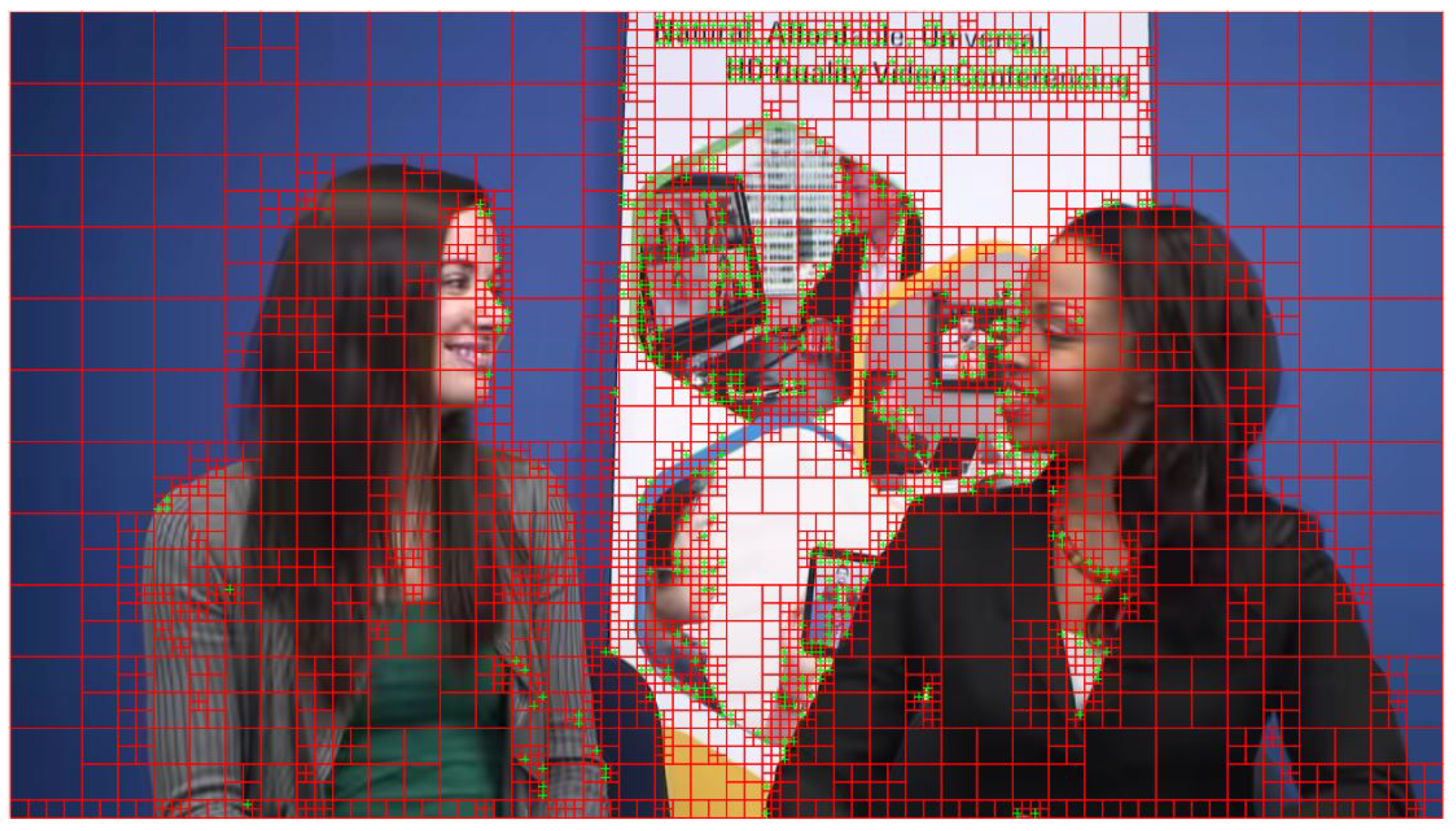
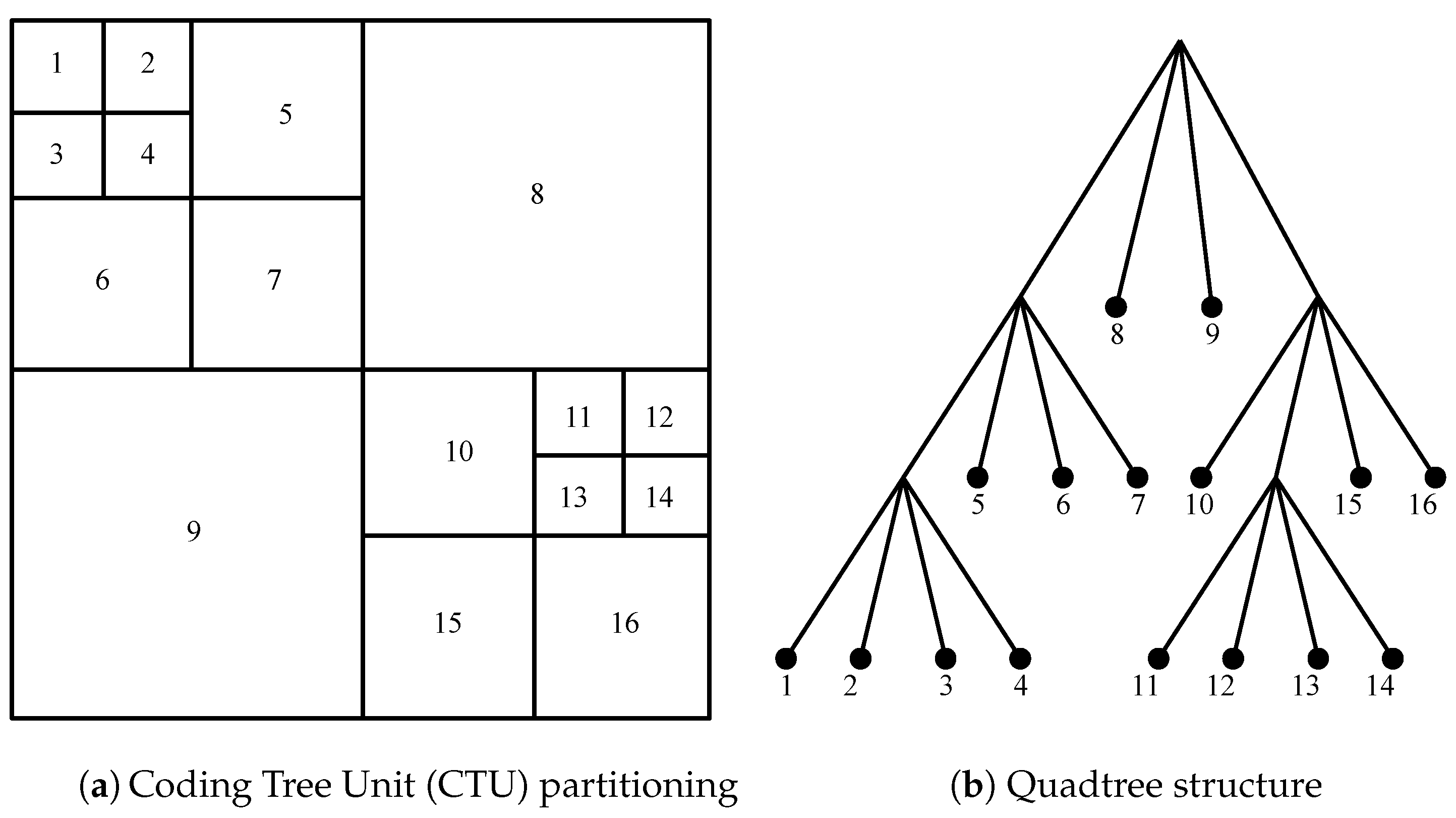
The block-based structure employed in HEVC initially partitions a given frame into CTUs, which have the size . Each CTU can then be recursively subdivided into CUs, ranging from to . For example, Figure 1 illustrates a typical partitioning structure for an encoded frame. Figure 2a shows a CTU which is recursively partitioned into multiple CUs, while Figure 2b depicts the corresponding hierarchical quadtree structure. In addition, a CU can be further partitioned into multiple Prediction Units (PU) and Transform Units (TU) to hold prediction and transform information, respectively [6]. The increased number of partitioning combinations available for a CTU in the HEVC standard requires the HEVC compatible encoders to determine the optimal partitioning structures for a given content. A typical encoder in this case follows a brute-force approach of evaluating all possible coding parameter combinations using RD optimisation to determine the optimum set of coding parameter combination for a given content.
RD optimisation utilises a Lagrangian cost function to evaluate the RD cost of each coding mode; and a partitioning structure to select the coding parameter combination that results in the minimum cost. This cost function can be expressed as
where is the Lagrange multiplier, p is a coding parameter combination from the set of all the possible coding options P, and , are the distortion and rate associated with the selected set of coding parameters, respectively [4]. Although this process enables identifying the highest attainable coding efficiency, it is one of the main sources of encoding complexity in the encoder. Thus, recent literature has focused on algorithms to minimise the computational complexity involved in the brute-force RD computation cost while keeping the coding performance intact. As part of this, more attention is given to the fast selection of CU structure since a large portion of the encoding time is devoted to the computations that take place at CU level [5].
2.2. Related Work
The state-of-the-art encoding algorithms that focus on fast CU size selection can be broadly categorised into three main categories—statistical rule-based approaches, texture properties-based algorithms, and machine learning-based approaches. The fast encoding algorithms proposed in the literature for intra-prediction typically focus on fast CU size selection or early estimation of optimal prediction mode (out of 35 intra-prediction modes [16]). The following subsections provide a summary of the existing work in each of these categories, primarily focusing on fast CU size selection algorithms available in the literature.
2.2.1. Statistical Rule-Based Methods
Rule-based models typically make use of statistical models generated from the content and data collected during the encoding loop. For example, Cho et al. and Kim et al. [9] applied a Bayesian decision rule to early prune the recursive CU evaluation process. Data accumulated during the encoding process such as RD costs, prediction residuals, distribution of RD cost in neighbouring blocks, and CU structures in neighbouring blocks are often treated as important features when determining the early termination of the current CU evaluation. For example, RD cost of the current CU is compared with a predetermined threshold to early terminate the encoding process of a CU in [17]. However, fixed thresholds and less flexible decision trees of these algorithms make the encoding decisions less content-adaptive. Most probable CU depth is determined using the spatial correlation among neighbouring CUs in [18,19]. A similar correlation analysis is carried out between Base and Enhancement Layers of Scalable HEVC (SHVC) to achieve fast intra-coding in [20]. Statistical properties of neighbouring PUs are considered to avoid evaluation of all 35 intra-prediction modes in [21]. In the meantime, Zhang et al. [22] introduce a combined use of statistical properties and Hadamard cost in Rough Mode Decision (RMD) to select both CU size and prediction mode for the PU. In addition, RMD costs are also utilised in [23] to make subsequent CU split decisions. Following a similar approach by Kim et al. [17], the CU is split to the next depth level straight away without processing the current level if the RMD cost exceeds a predefined threshold. However, diversity of content and large numbers of prediction modes and CU size combinations make the estimation of accurate CU sizes a compelling challenge with a small number of features and rigid thresholds. Further to that, unnecessary evaluation of the current CU depth level, rigid less flexible decision trees, and limited encoding time reduction achieved are identified as common drawbacks in these approaches. The use of CU information from the parent CU is often seen in methods that focus on improving the complexity reduction of inter-prediction. For example, Pan et al. [24] propose a complexity reduction algorithm for Versatile Video Coding (VVC), by adaptively determining the search range for CUs and the reference frame directions, based on the parent CU information. Furthermore, a complexity reduction algorithm is proposed in [25], where fractional pixel motion estimation of sub-PUs are skipped based on the motion estimation result of the parent CU. However, these methods utilise the features extracted from the inter-picture prediction process. Therefore, these methods cannot be applied in the context of intra-picture prediction complexity reduction.
2.2.2. Texture Properties-Based Methods
There is a clear correlation between the CU size selected and the texture complexity of the video frame. For example, there is a tendency to use larger CUs in homogeneous regions of a video frame; whereas less homogeneous regions tend to use smaller CUs (e.g., Figure 1). Following a similar principle, Lokkoju et al. [26] propose to use gradient information computed using horizontal and vertical Sobel kernels to compute the CU split decision. Further to that, texture complexity computed from directional gradients is compared with a QP dependent adaptive threshold to determine the partitioning structure for a given content in [27]. A similar content-adaptive threshold determination is followed in [28] when determining the early termination of the recursive CU partitioning process. Shen et al. in [29] and Min et al. in [30] follow similar approaches that consider texture homogeneity and directional edge complexities, respectively, to determine the CU size. Texture features of the spatial CUs and co-located CU are used in [31] for fast CU size decisions in 3D-HEVC. Furthermore, texture edges identified using Sobel kernels are utilised to early predict the angular prediction direction in HEVC intra-prediction in [32]. However, in general, kernel-based gradient computation used in these algorithms is seen as a time-consuming operation resulting in a limited encoding time reduction. Therefore, Mallikarachchi et al. in [33] propose to use local range as a texture complexity measurement when determining the CU size for given video content. However, the predetermined threshold and rigid decision trees make this algorithm less content-adaptive leading to inefficient CU size decisions for arbitrary sequences.
2.2.3. Machine Learning-Based Methods
Machine learning-based methods, on the other hand, utilise supervised learning algorithms to learn the model parameters using the data collected from encoded video sequences to provide optimal discriminative solutions to the CU size selection problem. For instance, Convolutional Neural Network (CNN) has been proposed in [34] to assist in the early CU size selection in HEVC intra-coding. The algorithm proposed by Liu et al. does not rely on the spatial information, thereby facilitating parallel execution of the algorithm. However, use of a CNN as an inference engine adds up the complexity overhead of the decision-making process, which demands additional hardware acceleration elements. Following a different approach, Hu et al. [35] and Chen et al. [36] formulated CU size selection as a Bayesian classification problem. In this case, the former utilises Discrete Cosine Transform (DCT) coefficients; while the latter extends the classification to two-stage cascading classifiers. The three-class classifier used in the first stage in [36] groups the CUs into “split”, “non-split”, and “undecided” categories based on the dynamics of the feature space. In addition, the machine learning algorithms such as random forests and data mining techniques have been used in [37,38], respectively, to address the complexity reduction problem in HEVC intra-prediction. SVM classification is often considered as a popular machine learning algorithm for binary classification problems that can also mediate the resulting overhead complexity on the encoding loop. In this regard, [39] utilises two linear SVM models that employ the depth difference and HAD and RD cost ratio as features to perform the decisions of early CU split and early CU termination. Following a similar approach, Shen and Yu [14] propose an early termination algorithm for recursive CU evaluation using Support Vector Machines (SVMs). In addition, Zhang et al. [10] propose an early termination/early split mechanism where multiple SVMs are utilised. The two-stage approach proposed in [10] utilises offline trained models and weight parameters for the decision making process. However, the offline computation of SVM weights and hyperplane and support vectors make the CU split decisions obtained through the models less content-adaptive.
3. CU Split Likelihood Modelling Using SVMs
This section first introduces the concept of CU split decision in the HEVC quadtree partitioning structure. Next, the usage of SVMs to model the CU split likelihood as a binary classification problem is discussed, followed by an overview of SVMs and Weighted SVMs.
3.1. CU Split Likelihood Modelling
HEVC block-based encoding utilises a quadtree partitioning structure within a CTU. This enables the encoder to capture the local characteristics of the content when determining the optimum coding modes for a given content [3,6]. During this process, each CU is recursively partitioned into four equally-sized sub-CUs. The size of a CU can range from to , each layer of CU size representing a CU depth level (0, 1, 2, and 3). During the RD optimisation process, each CU depth level is evaluated for all corresponding PU modes and the best resultant RD cost is compared with the overall RD cost of the next available CU depth level. In this case, if the RD cost of the current CU becomes greater than the RD cost of the next CU depth level, a decision is made to split the current CU into four sub-CUs. On the other hand, the current CU is considered to remain non-split if the RD cost evaluates to be less than overall RD cost of its sub-CUs. This can be formulated as a binary classification problem to classify each CU into two classes (i.e., split and non-split), during the encoding phase as
Here, is the CU split decision, is the RD cost of the parent CU, is the RD cost of the a sub-CU where represents the CU size, and represents the CU depth level.
The split likelihood of a CU can be modelled using probabilistic models [7,35,36] as well as machine learning methods. In the case of the latter, recent literature typically uses supervised learning algorithms such as decision trees [17,38], neural networks [34], logistic regression, and SVMs [10,14,39]. However, integrating an inference engine of machine learning models into the encoding loop such that the time taken for decision making is minimal, is crucial a for fast CU size selection algorithms (such as proposed in this work). Therefore, this work utilises SVMs to model the CU split likelihood due to its ability to handle binary classification problems with significant computational advantages [40].
3.1.1. Support Vector Machines (SVMs)
SVM is a supervised machine learning method that is used in classification and regression problems [41,42]. It is often used as a non-probabilistic binary classifier that predicts the class for a given input vector. For example, let D be a training dataset of size n, where
Here, is a p-dimensional input vector and is the corresponding class to which each belongs. During the training phase, SVM constructs a hyperplane that represents the largest separation of the dataset D (known as the margin) in a higher-dimensional space, solving the primal optimisation function defined as
where w, , and are the normal vector to the hyperplane, slack variable, and regularisation parameter, respectively. Here, acts as the Kernel function that maps into a higher-dimensional space in the case of nonlinear classification. Once the hyperplane is determined, the classifications for the new samples are obtained using the decision function given by,
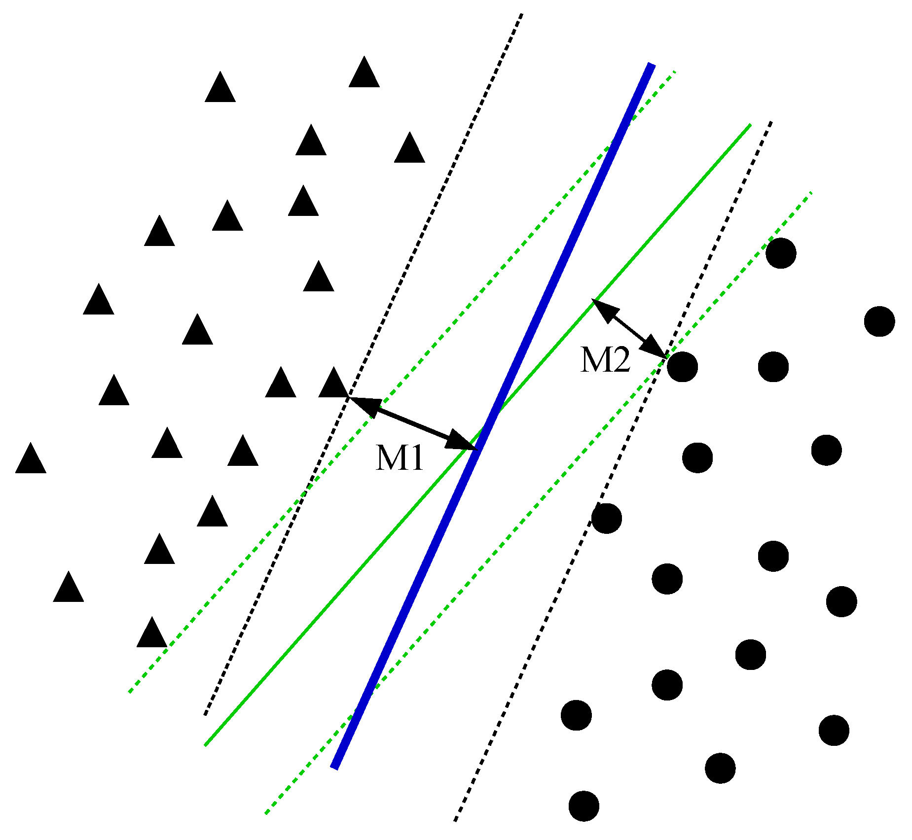
A typical separation of a dataset and a hyperplane (line in blue colour) that achieves the maximum possible hyperplane margin , where , is illustrated in the Figure 3.
3.1.2. Weighted Support Vector Machines (W-SVMs)
The empirical observations on the training data collected during the data collection phases in the proposed algorithm (Section 4.1.1 and Section 4.2.1) reveal that the dataset is often contaminated by noise. The dynamic nature of the video contents, diversity of texture, and motion complexities of typical video sequences result in certain data points being positioned on the wrong side in the feature space, generating a significant number of outliers. In the standard SVM [43], the classification gets affected when the outliers become support vectors in the decision boundary during the training phase (i.e., outlier sensitivity problem [44,45]).
In this context, Weighted Support Vector Machines (W-SVM) is seen as a potential solution which assigns weights to the training samples based on their relative importance [45]. Thus, the effect of less important points is reduced during the training phase. Following a similar approach, the training dataset utilised in the proposed method is trained with W-SVM using a modified constrained optimisation function given by
where —where , . Here, is the feature vector of the training set, with ith sample being represented as —where is the class label. Furthermore, w, , C, and are the hyperplane margin, slack variable, and trade-off parameter for hyperplane margin width and misclassification, and weight parameters for CU non-split and split classes, respectively.
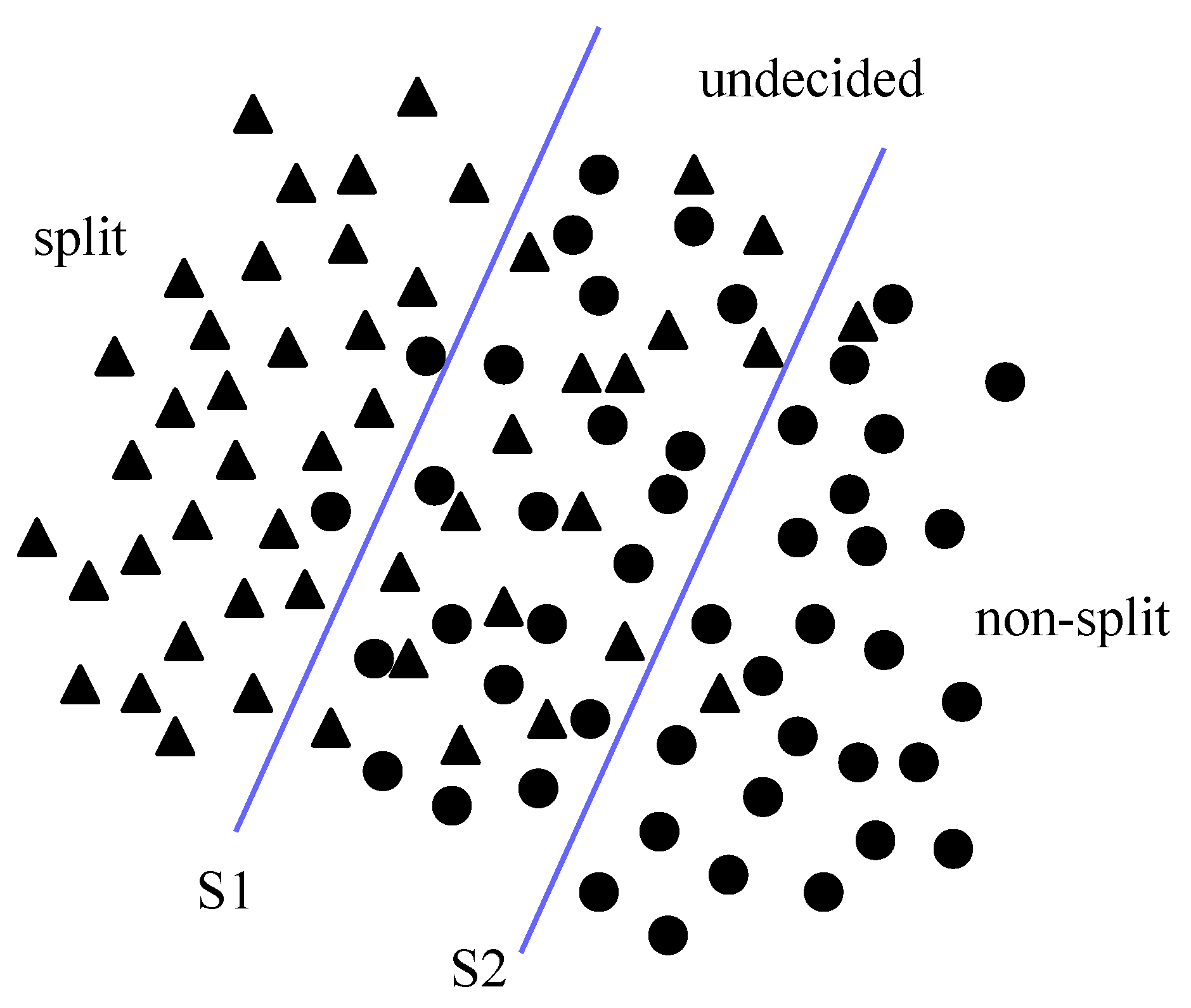
The use of different weights for samples (i.e., and , respectively) reduce the effect of less important data points (such as outliers and noise) when building the hyperplanes during the training phase. Figure 4 depicts an illustration of two hyperplanes generated for two SVM models by applying different weights for split and non-split samples in the training dataset (refer Section 4).
4. Proposed Fast CU Size Selection Algorithm
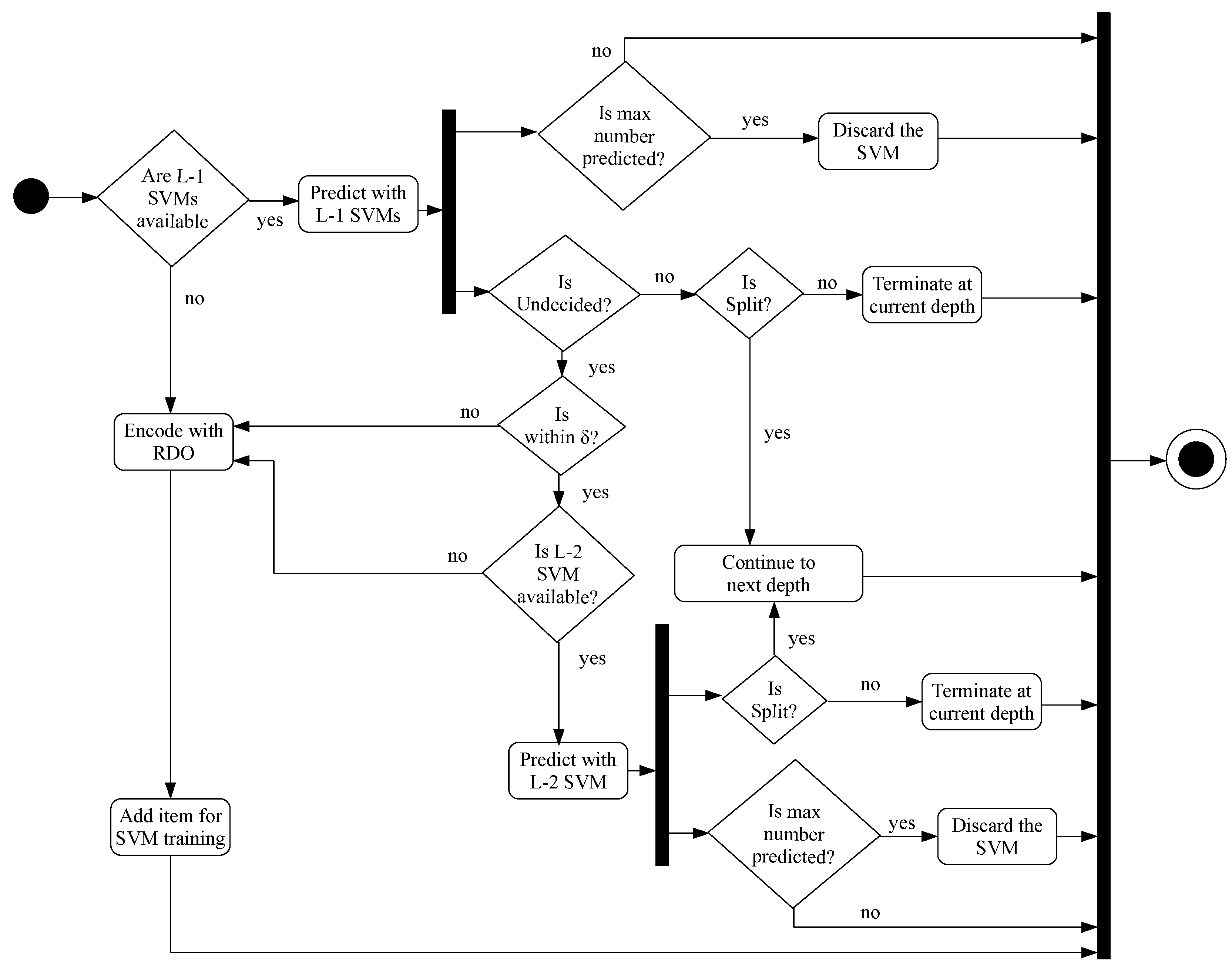
The proposed method utilises SVM models at two levels in the HEVC coding architecture. The SVM models at level 1(L-1) are generated and utilised before the encoding of the current CU depth level (See Figure 5). The SVM model at level 2 (L-2) is generated and used after the evaluation of the CU for the PU modes at the current CU depth level. The following section describes the data collection, feature selection, and model parameter computations carried out in the proposed algorithm on both these levels.
4.1. Level 1(L-1) SVM Models: Features and Optimal Weight Calculation
As illustrated in Section 2, the typical machine learning approaches rely on large data sets of coding information and CU split decisions for a selected number of training video sequences to build and train generic offline models. However, the dynamic nature of the video contents and diversity of required quality levels make these generic models less flexible and less effective when applying them to estimate encoding decisions. Hence, the proposed method relies on coding, texture, and statistical information accumulated online during the encoding process and dynamically generate SVM models which are unique for a given content. The following subsections illustrate the feature selection and SVM weight calculation utilised with the L-1 SVM models in the proposed method.
4.1.1. Data Collection
L-1 constitutes two weighted SVM models (Section 3.1.2) for each CU depth level using the data collected during an initial training phase for each video sequence. During the initial training phase, N data points are accumulated for each CU depth level (i.e., 0, 1, 2, 3). In this phase, CU/PU size decisions are obtained through traditional RD optimisation.
Here, N is set at , which gives the best trade-off between the encoding time reduction and model accuracy based on the empirical observation.
The SVM models for a particular CU depth level are generated once the required N number of data points are collected during the encoding process. This enables the models to be generated at different times depending on the content, resolution, and Quantisation Parameter (QP). For example, SVM models for lower CU depths (i.e., 0, 1) for certain sequences with low resolution (e.g., 416 × 240) are typically generated after encoding several frames, whereas SVM models for higher CU depths (i.e., 2, 3) typically become available much sooner.
The ratio between the training and predicted samples is kept at 1:. Once the number of predictions per model () is exceeded, the model is expired and recreated following a similar data collection approach. This process ensures the SVM models are kept relevant to the content being encoded and are hence, content-adaptive. In this case, is maintained as , which results in a minimal BDBR increase for a set of test video sequences evaluated at for a range of ratios where . Experimental results reveal that the models for smaller CU sizes are retained for a longer period of time before they are discarded when encoding less complex, high-resolution sequences using large QPs. This is due to the lower presence of smaller CUs in such scenarios. Similar behaviour is observed for the SVM models corresponding to large CU sizes when encoding complex sequences using smaller QPs. Retaining models for a longer period impacts the content adaptiveness of the SVM models and results in coding efficiency losses. However, the lower number of decisions made by such models facilitates the algorithm to maintain any adverse impacts on the coding efficiency at a lower level. In this context, remains a design parameter that can trade-off the encoding time reduction to the coding efficiency, depending on the requirement.
4.1.2. Feature Selection
Let be the set of features extracted for CU depth i in the j-th level. Therefore, at L-1, is defined as
where, , , and correspond to the texture complexity, RD cost pre-analysis of current CU, and context information, respectively, for the ith CU depth level [10]. In this case, the texture complexity () is calculated using the mean absolute difference () of the current CU and the texture difference between the current CU and its four sub CUs (). RD cost pre-analysis includes division between the RD cost and QP () and division between RD cost and distortion (). In this case, RD cost is calculated by encoding the CU with planar intra mode. The RD cost (), CU depth (), and PU depths () of the spatially neighbouring above and left CTUs are extracted as context information features for the [10]. Different combinations of these features are utilised at different depth levels, as depicted in Table 1.
4.1.3. Weight Calculation
The weight parameters for L-1 SVM models (that utilise the objective function in (6)) are defined such that highest attainable precision is achieved for a particular decision. In this case, the precision for the two SVMs () for the ith CU depth level is defined as
and
Here, , are the “True Positive”, and “True Negative” samples, whereas and are the “False Positive” and “False Negative” samples, respectively. In addition, and identify the SVM decision models that carry more weight into CU “split” and “non-split” decisions, respectively, with maximum confidence using the optimisation function defined in (6). Maximising the precision for model results in minimising the categorisation of “non-split” samples as “split”. At the same time, maximising the precision for minimises the categorisation of “split” samples as “non-split”. The logical separation of the samples, SVM models, and corresponding hyperplanes for a particular CU depth level are illustrated in Figure 4.
The optimal weight parameters ( and in (6)) for each of the SVM models ( and ) are determined at run time after the data collection (described in Section 4.1.1) is complete for a particular depth level. Here, weight value pairs ranging from 5:1 (:) and 1:5 (:) with a step size of 0.5 are evaluated for and SVM models, respectively. Then, the weight pair that achieves the highest precision in (8) and (9) for and , respectively, is selected for the corresponding optimisation function in (6). Here, the data points collected are equally divided to form training and cross-validation sets. For optimal weight calculation for the SVMs, cross-validation is done over predetermined weight value pairs to ensure that time consumed for the process is minimised. The kernel function selected for the SVMs is Radial Basis Function (RBF), given its ability to work efficiently with small numbers of features while performing well with nonlinear decision boundaries [46]. In order to minimise the impact of model tuning time during the encoding process, other hyper-parameters with RBF kernel, i.e., cost parameter, gamma parameter, and the number of training samples, are predetermined and are not tuned during the model building process. The cost parameter is set at 100, giving a large penalty for misclassification, when compared with the default value of 1. The value for gamma is set at the default value, i.e., for each model.
4.2. Level 2 SVMs (L-2): Features and Optimal Weight Calculation
The SVM model at L-2 is built and utilised after PU modes are evaluated for the current CU depth level. In terms of the overall encoding algorithm (Figure 5), the CU split decisions that are not classified by the L-1 SVMs are subjected to the L-2 SVM model. In this case, a single SVM is used at each CU depth level.
4.2.1. Data Collection
The number of training samples collected for the L-2 is maintained at for each CU depth level. In this case, the number of training samples to be used are determined empirically, which achieves the best trade-off between the encoding time reduction and model accuracy. Similar to L-1 models, L-2 models at each CU depth level are discarded once a certain number of predictions are made. In this case, existing L-2 models are discarded and recreated with a new data set keeping the ratio between the training and predicted samples at 1:200. This ensures that the models generated are content-adaptive and CU size predictions are content relevant. Similar to the L-1, the ratio is selected empirically, following the same process described in Section 4.1.1.
4.2.2. Feature Selection
Let be the set of features extracted for the ith CU depth level in jth level. Thus, for level 2, is defined as
where , , and refer to texture information, context-information, and coding information, respectively, for the ith CU depth level [10]. In this case, the texture complexity is calculated with the mean absolute difference of the block (). The context information for L-2 includes the sum of the CU depths () and the average of the sum of CU and PU depth levels () from the left and above neighbouring CTUs. The coding information for L-2 includes the RD cost () and the number of bits (). Since the current depth level is already considered in the first level, data that is directly related to the CU are available in the second level. Similar to L-1, different combinations of the features [10] are used at the depth levels, as shown in the Table 2.
4.2.3. Weight Calculation
The weight parameters for L-2 SVMs that utilise the objective function in (6) are obtained by following a similar approach as defined in Section 4.1.3. In this case, a range of weights varying from 1:5 (:) and 5:1 (:), with 0.5 step size difference at each iteration, are tested during run-time. Level 2 SVM models are used to classify CUs either as “non-split” or “split”. As only one SVM is used at the second level, it is not possible to address only one case—either split or non-split. Therefore, we calculate the F-score for the cross-validation set to determine the best weight parameters. Here, training and cross-validation sets are derived following the same method explained in the first level (Section 3.1). The F-score calculation is given by
where and are precision and recall, respectively. Here, recall is calculated using
The pair of weights that gives the highest possible F-score is chosen for the SVM at the corresponding depth level. The kernel function used in the SVMs is RBF and similar to the hyper-parameters in L-1, although the weights are fine-tuned to minimise the adverse impact on the time gains by the model training during the encoding process. The cost and gamma parameters are the same as those in L-1.
4.3. Overall Encoding Algorithm
The overall fast encoding algorithm proposed in this manuscript is illustrated in Figure 5. As illustrated, the proposed method first builds the SVMs using RDO and operates in two levels—before encoding the current depth; and after encoding the current depth.
The SVM models generated at L-1 predict the CU’s “split” () and “non-split” () decisions for a given CU depth level . As illustrated in Figure 5, the CU size decisions that cannot be predicted by the L-1 SVMs are subjected to the L-2 SVMs. For example, any CU that is classified into the middle region identified in the Figure 4, is evaluated for all its PU modes and passed on to L-2 model to determine whether to further split the CU or select the current CU size as it is.
Complexity Control Parameter ()
The proposed method introduces a complexity control parameter to allow number of CUs that reach L-2 models to go through traditional RD-optimisation, to determine their CU split decisions. Controlling in the proposed algorithm facilitates the flexibility to trade-off coding complexity to the coding efficiency.
5. Experimental Results and Discussion
The following section presents the experimental results of the proposed fast CU size selection and encoding algorithm for HEVC video encoding. The proposed algorithm is implemented in HM16.1 [15], and the optimised SVM library libSVM [46] is used to implement the SVM models described in Section 4. The RD and encoding time performance of the proposed algorithm are compared with several state-of-the-art algorithms in the literature. These include HM16.1 [15], SVM-based CU size selection algorithm proposed by Zhang et al. [10], and fast CU selection algorithms proposed by Liu et al. [34].
5.1. Experimental Setup and Encoding Configurations
The algorithms are evaluated for a range of HD and UHD video sequences composed of content ranging from simple to highly complex motion with diverse spatial and temporal characteristics. The video sequences, encoding configurations, and QP values are selected as defined in the HEVC common test configurations [47]. For instance, test sequences are encoded using All intra main configuration for . All experiments are carried out in an AMD 64-Core CPU @ 2.5 GHz system with 64 GB RAM and Ubuntu 14.04 64-bit operating system.
The average percentage encoding time reduction, , is evaluated for the proposed and state-of-the-art algorithms by
where is the encoding time of HM reference software and is the encoding time required for each fast encoding approach. For the proposed method, includes the time taken for the data collection, feature extraction, computing weights, and online-SVM training.
The coding efficiency performance of the proposed and state-of-the-art algorithms is measured against the HM reference encoder using Bjøntegaard Delta Bit Rate (BDBR) [48]. In this case, BDBR is computed using two different quality metrics. First, Peak Signal to Noise Ratio (PSNR)—a widely used objective quality metric—is used as the quality metric in the RD curve. Then, Video Quality Metric (VQM) tools that estimate the perceived video quality of the users is utilised as the quality metric when computing the BDBR [49]. The perception of visual media is influenced by the Human Visual System, the brain, and the eye [50]. Typically, a human observer gives higher importance to certain parts of a picture, as opposed to giving equal importance to every part. Objective quality metrics such as PSNR fail to capture the perceived subjective quality in such scenarios. On the contrary, VQM is widely considered as a calibrated model of subjective video quality measurement that closely correlates to the user’s QoE when consuming video content [51].
5.2. Results and Performance Analysis
The experimental results presented in Table 3 and Table 4 demonstrate coding performance and encoding time reduction of the proposed and state-of-the-art methods against HEVC HM16.1 implementation when using PSNR and VQM as the quality metrics, respectively. The following section discusses the overall performance and implications of using the proposed fast coding framework.
5.2.1. Impact of Complexity Control Parameter
The ability of the proposed algorithm to trade-off the coding efficiency to the encoding complexity by adjusting the complexity control parameter is a crucial advantage compared to the state-of-the-art methods, which use fixed thresholds and rigid decision trees to derive the CU size decision. Increasing allows the encoder to increase the coding efficiency, at the expense of increased encoding time and vice-versa. Thus, becomes an engineering design parameter which is tuned depending on the user requirement. In this case, the experimental results presented in this paper correspond to values maintained at and .
5.2.2. Overall Performance Analysis
It can be observed from the Table 3 and Table 4, that the proposed method at demonstrates a significant encoding time complexity reduction with a lower impact on the measured objective and subjective quality, compared to the implementation presented in [10]. The algorithm proposed by Liu et al. [34] shows a slightly higher encoding time gain at a higher visual quality impact. The proposed method with records the highest encoding complexity reduction, with an average of .
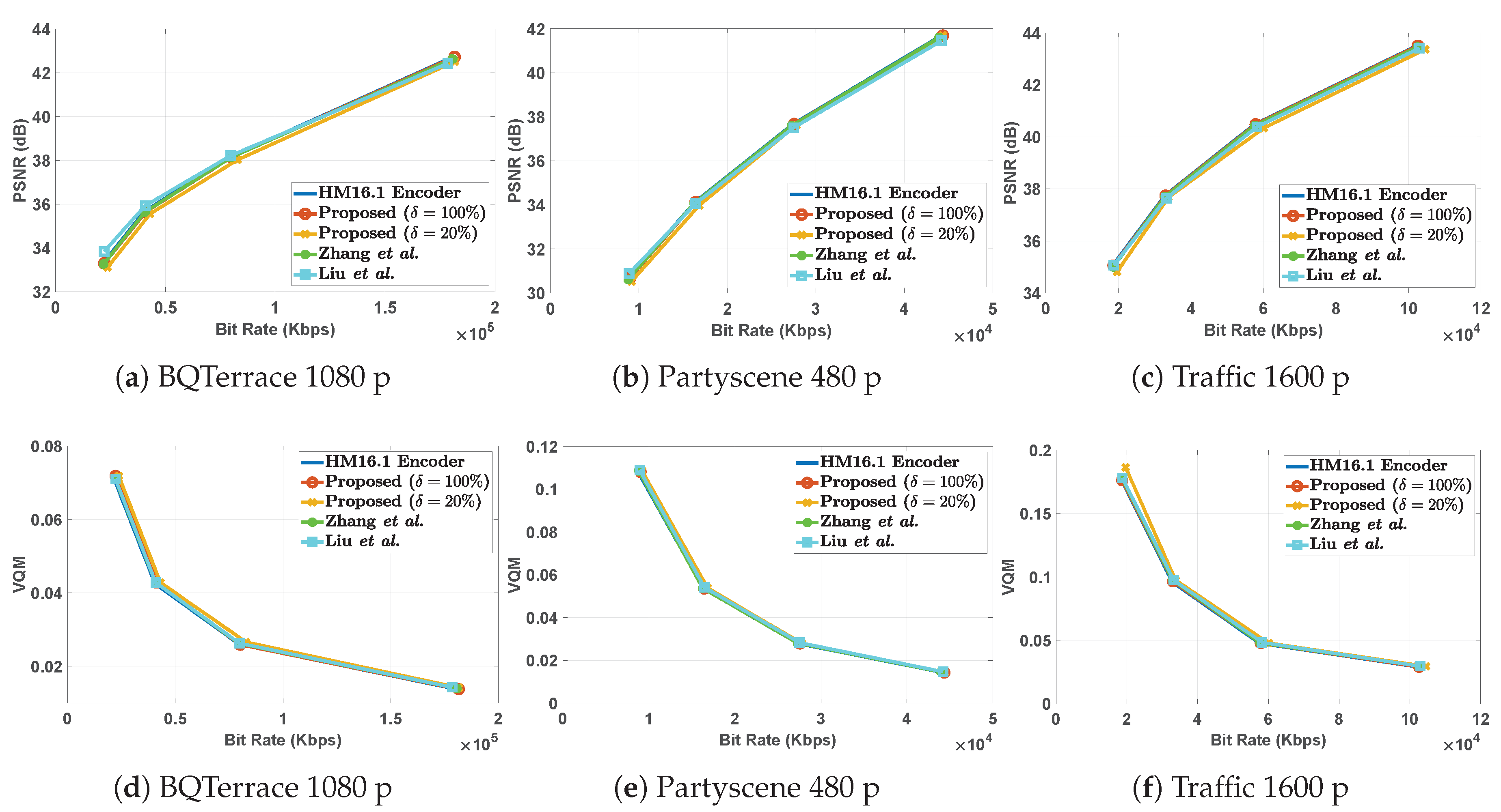
The high visual quality degradation and fixed time gains of [34] can be attributed to the rigid models used in the approach. Similarly, the fixed time complexity reductions in [10] are a result of the offline and fixed-threshold models, that do not continuously adapt to the changing nature of the video content. The proposed method, on the contrary, makes use of content-adaptive models with the complexity control parameter that can be tuned by the user. This allows higher time complexity reductions, while also keeping the encoding quality intact. Furthermore, it gives the flexibility to the user to trade-off the computational complexity with the encoding efficiency according to individual application requirements. In addition, the RD performance graphs for the bit streams generated by the proposed algorithm depicted in Figure 6 demonstrate similar coding efficiency performance to that of the bit streams generated by the HM16.1 reference encoder implementation.
6. Conclusions
In this paper, we propose a fast content-adaptive CU size selection mechanism using weighted SVMs. The proposed SVM models are utilised at two different levels in the HEVC encoding chain. First, level-1 SVM models are used before the encoding of the current CU to determine whether to skip the current level or to encode the current CU level. This early CU size decision eliminates the evaluation of unnecessary CU sizes, thus, enabling the proposed algorithm to achieve significant encoding time reductions. The CU size decisions that cannot be classified as “split” or “non-split” with the level-1 SVM models are passed on to level-2 SVM model which operates once the current CU level is evaluated for all the possible PU modes. The level 2 SVM model then decides whether to continue the recursive splitting of the CU or move on to the next coding block.
The proposed method collects data and builds models in run-time during the encoding process, which makes the CU split decisions derived using the proposed algorithm dynamic and content-adaptive—a crucial advantage compared to the state-of-the-art methods that rely on large amounts of past data. The complexity control parameter introduced in this work allows the proposed algorithm to control the amount of decisions taken by the SVM models and traditional RD optimisation, thereby effectively trading-off the computational complexity to the coding efficiency. The experimental results reveal an average encoding time saving of up to 52.38%, with only 1.19% average BDBR increase (i.e., increase in bitrate to a similar video quality by the proposed algorithm) compared to the HM16.1 encoded bit streams, when using PSNR as the quality measurement for the reconstructed videos. Similarly, the proposed algorithm demonstrates 1.52% average BDBR increase compared to HM encoded streams when measuring the users’ perceived video quality using VQM. Therefore, the proposed algorithm provides an effective alternative compared to the state-of-the-art algorithms to reduce the encoding time complexity of HEVC intra-coding in emerging multimedia applications.
The future works will focus on extending the framework for HEVC inter-prediction to facilitate fast content-adaptive HEVC video coding.
Author Contributions
Conceptualization, B.E. and T.M.; methodology, B.E; software, B.E.; validation, B.E. and T.M.; formal analysis, B.E. and T.M.; investigation, B.E.; resources, A.F. and C.H.; data curation, B.E.; writing—original draft preparation, T.M.; writing—review and editing, T.M., B.E., and C.H.; visualization, T.M.; supervision, T.M., A.F.; project administration, A.F.; funding acquisition, A.F. and C.H.
Funding
This research was funded by the CONTENT4ALL project, which is funded under European Commission’s H2020 Framework Program (Grant number: 762021) and European Social Fund (ESF) grant under KESSII WEST – Collaborative project between Cardiff Metropolitan University and Ultranyx Ltd.
Conflicts of Interest
The authors declare no conflict of interest.
References
- Cisco. Cisco Visual Networking Index: Global Mobile Data Traffic Forecast Update 2014–2019; White Paper; Cisco: San Jose, CA, USA, 2017. [Google Scholar]
- Segall, A.; Wien, M.; Baroncini, V.; Boyce, J.; Suzuki, T. Draft Joint Call for Proposals on Video Compression with Capability beyond HEVC. In Proceedings of the Joint Video Exploration Team (on Future Video Coding) of ITU-T VCEG and ISO/IEC MPEG, 7th Meeting, Torino, IT, USA, 13–21 July 2017. [Google Scholar]
- Sullivan, G.J.; Ohm, J.; Han, W.J.; Wiegand, T. Overview of the High Efficiency Video Coding (HEVC) Standard. IEEE Trans. Circuits Syst. Video Technol. 2012, 22, 1649–1668. [Google Scholar] [CrossRef]
- Ohm, J.R.; Sullivan, G.J.; Schwarz, H.; Tan, T.K.; Wiegand, T. Comparison of the coding efficiency of video coding standards—Including high efficiency video coding (HEVC). IEEE Trans. Circuits Syst. Video Technol. 2012, 22, 1669–1684. [Google Scholar] [CrossRef]
- Bossen, F.; Bross, B.; Karsten, S.; Flynn, D. HEVC complexity and implementation analysis. IEEE Trans. Circuits Syst. Video Technol. 2012, 22, 1685–1696. [Google Scholar] [CrossRef]
- Kim, I.K.; Min, J.; Lee, T.; Han, W.J.; Park, J. Block Partitioning Structure in the HEVC Standard. IEEE Trans. Circuits Syst. Video Technol. 2012, 22, 1697–1706. [Google Scholar] [CrossRef]
- Mallikarachchi, T.; Talagala, D.S.; Arachchi, H.K.; Fernando, A. Content-Adaptive Feature-Based CU Size Prediction for Fast Low-Delay Video Encoding in HEVC. IEEE Trans. Circuits Syst. Video Technol. 2016, 28, 693–705. [Google Scholar] [CrossRef] [Green Version]
- Baroncini, V.; Ferrara, S.; Ye, Y. Call for Proposals for Low Complexity Video Coding Enhancements; International Organization for Standardization, Coding of Moving Pictures and Audio, ISO/IEC JTC1/SC29/WG11/ N17944; International Organization for Standardization: Geneva, Switzerland, 2018. [Google Scholar]
- Cho, S.; Kim, M. Fast CU splitting and pruning for suboptimal CU partitioning in HEVC intra coding. IEEE Trans. Circuits Syst. Video Technol. 2013, 23, 1555–1564. [Google Scholar] [CrossRef]
- Zhang, Y.; Pan, Z.; Li, N.; Wang, X.; Jiang, G.; Kwong, S. Effective Data Driven Coding Unit Size Decision Approaches for HEVC INTRA Coding. IEEE Trans. Circuits Syst. Video Technol. 2017, 28, 3208–3222. [Google Scholar] [CrossRef]
- Khan, M.U.K.; Shafique, M.; Henkel, J. An adaptive complexity reduction scheme with fast prediction unit decision for HEVC intra encoding. In Proceedings of the IEEE International Conference on Image Processing (ICIP), Melbourne, VIC, Australia, 15–18 September 2013; pp. 1578–1582. [Google Scholar]
- Zhang, Y.; Kwong, S.; Wang, X.; Yuan, H.; Pan, Z.; Xu, L. Machine learning-based coding unit depth decisions for flexible complexity allocation in high efficiency video coding. IEEE Trans. Image Process. 2015, 24, 2225–2238. [Google Scholar] [CrossRef]
- Correa, G.; Assuncao, P.; Agostini, L.V.; Silva, L.A.C. Fast HEVC encoding decisions using data mining. IEEE Trans. Circuits Syst. Video Technol. 2015, 25, 660–673. [Google Scholar] [CrossRef]
- Shen, X.; Yu, L. CU splitting early termination based on weighted SVM. EURASIP J. Image Video Process. 2013, 2013, 4. [Google Scholar] [CrossRef]
- HM 16.1. Available online: https://hevc.hhi.fraunhofer.de/trac/hevc/browser/tags/HM-16.1 (accessed on 15 January 2019).
- Lainema, J.; Bossen, F.; Han, W.J.; Min, J.; Ugur, K. Intra coding of the HEVC standard. IEEE Trans. Circuits Syst. Video Technol. 2012, 22, 1792–1801. [Google Scholar] [CrossRef]
- Kim, J.; Choe, Y.; Kim, Y.G. Fast coding unit size decision algorithm for intra coding in HEVC. In Proceedings of the IEEE International Conference on Consumer Electronics (ICCE), Las Vegas, NV, USA, 11–14 January 2013; pp. 637–638. [Google Scholar]
- Shen, L.; Zhang, Z.; An, P. Fast CU Size Decision and Mode Decision Algorithm for HEVC Intra Prediction. IEEE Trans. Consum. Electron. 2013, 59, 207–213. [Google Scholar] [CrossRef]
- Zhang, Y.; Kwong, S.; Zhang, G.; Pan, Z.; Hui, Y.; Jiang, G. Low complexity HEVC INTRA coding for high-quality mobile video communication. IEEE Trans. Ind. Inf. 2015, 11, 1492–1504. [Google Scholar] [CrossRef]
- Zuo, X.; Yu, L. Fast mode decision method for all intra spatial scalability in SHVC. In Proceedings of the 2014 IEEE Visual Communications and Image Processing Conference, Valletta, Malta, 7–10 December 2014; pp. 394–397. [Google Scholar]
- Wang, L.L.; Siu, W.C. Novel adaptive algorithm for intra prediction with compromised modes skipping and signaling processes in HEVC. IEEE Trans. Circuits Syst. Video Technol. 2013, 23, 1686–1694. [Google Scholar] [CrossRef]
- Zhang, H.; Ma, Z. Fast intra mode decision for High Efficiency Video Coding (HEVC). IEEE Trans. Circuits Syst. Video Technol. 2014, 24, 660–668. [Google Scholar] [CrossRef]
- Zhang, H.; Ma, Z. Early Termination Schemes for Fast Intra Mode Decision in High Efficiency Video Coding. In Proceedings of the IEEE International Symposium on Circuits and Systems (ISCAS), Beijing, China, 19–23 May 2013; pp. 45–48. [Google Scholar]
- Pan, Z.; Qin, H.; Yi, X.; Zheng, Y.; Khan, A. Low complexity versatile video coding for traffic surveillance system. Int. J. Sens. Netw. 2019, 30, 116–125. [Google Scholar] [CrossRef]
- Pan, Z.; Lei, J.; Zhang, Y.; Wang, F.L. Adaptive fractional-pixel motion estimation skipped algorithm for efficient HEVC motion estimation. ACM Trans. Multimed. Comput. Commun. Appl. (TOMM) 2018, 14, 12. [Google Scholar] [CrossRef]
- Lokkoju, S.; Reddy, D. Fast coding unit partition search. In Proceedings of the IEEE International Symposium on Signal Processing and Information Technology (ISSPIT), Ho Chi Minh City, Vietnam, 12–15 December 2012; pp. 315–319. [Google Scholar]
- Zhang, Y.; Li, Z.; Li, B. Gradient based fast decision for intra prediction. In Proceedings of the IEEE Visual Communications and Image Processing (VCIP), San Diego, CA, USA, 27–30 November 2012; pp. 1–6. [Google Scholar]
- Tian, G.; Goto, S. Content Adaptive Prediction Unit Size Decision Algorithm for HEVC Intra Coding. In Proceedings of the Picture Coding Symposium (PCS), Krakow, Poland, 7–9 May 2012; pp. 405–408. [Google Scholar]
- Shen, L.; Zhang, Z.; Liu, Z. Effective CU size decision for HEVC intra coding. IEEE Trans. Image Process. 2014, 23, 4232–4241. [Google Scholar] [CrossRef]
- Min, B.; Cheung, R.C.C. A fast CU size decision algorithm for the HEVC intra encoder. IEEE Trans. Circuits Syst. Video Technol. 2015, 25, 892–896. [Google Scholar]
- Park, C.S. Efficient intra-mode decision algorithm skipping unnecessary depth-modelling modes in 3D-HEVC. Electron. Lett. 2015, 51, 756–758. [Google Scholar] [CrossRef]
- Zhang, Q.; Huang, X.; Wang, X.; Zhang, W. A fast intra mode decision algorithm for HEVC using sobel operator in edge detection. Int. J. Multimed. Ubiquitous Eng. 2015, 10, 81–90. [Google Scholar] [CrossRef]
- Mallikarachchi, T.; Fernando, A.; Arachchi, H.K. Efficient coding unit size selection based on texture analysis for HEVC intra prediction. In Proceedings of the IEEE International Conference on Multimedia and Expo (ICME), Chengdu, China, 14–18 July 2014; pp. 1–6. [Google Scholar]
- Liu, Z.; Yu, X.; Gao, Y.; Chen, S.; Ji, X.; Wang, D. CU Partition Mode Decision for HEVC Hardwired Intra Encoder Using Convolution Neural Network. IEEE Trans. Image Process. 2016, 25, 5088–5103. [Google Scholar] [CrossRef] [PubMed]
- Hu, N.; Yang, E.H. Fast mode selection for HEVC intra-frame coding with entropy coding refinement based on a transparent composite model. IEEE IEEE Trans. Circuits Syst. Video Technol. 2015, 25, 1521–1532. [Google Scholar] [CrossRef]
- Chen, J.; Yu, L. Effective HEVC intra coding unit size decision based on online progressive Bayesian classification. In Proceedings of the IEEE International Conference on Multimedia and Expo (ICME), Seattle, WA, USA, 11–15 July 2016; pp. 1–6. [Google Scholar]
- Du, B.; Siu, W.C.; Yang, X. Fast CU partition strategy for HEVC intra-frame coding using learning approach via random forests. In Proceedings of the 2015 Asia-Pacific Signal and Information Processing Association Annual Summit and Conference (APSIPA), Hong Kong, China, 16–19 December 2015; pp. 1085–1090. [Google Scholar]
- Coll, D.R.; Adzic, V.; Escribano, G.F.; Kalva, H.; Martínez, J.L.; Cuenca, P. Fast partitioning algorithm for HEVC intra frame coding using machine learning. In Proceedings of the 2014 IEEE International Conference on Image Processing (ICIP), Paris, France, 27–30 October 2014; pp. 4112–4116. [Google Scholar]
- Zhang, T.; Sun, M.T.; Zhao, D.; Gao, W. Fast intra-mode and CU size decision for HEVC. IEEE Trans. Circuits Syst. Video Technol. 2016, 27, 1714–1726. [Google Scholar] [CrossRef]
- Shawe-Taylor, J.; Cristianini, N. An Introduction to Support Vector Machines and Other Kernel-Based Learning Methods; Cambridge University Press: Cambridge, UK, 2000; Volume 204. [Google Scholar]
- Kecman, V. Learning and Soft Computing: Support Vector Machines, Neural Networks, and Fuzzy Logic Models; The MIT Press: Cambridge, MA, USA; London, UK, 2001. [Google Scholar]
- Schölkopf, B.; Smola, A.J. Learning with Kernels: Support Vector Machines, Regularization, Optimization, and Beyond; The MIT Press: Cambridge, MA, USA; London, UK, 2002. [Google Scholar]
- Cortes, C.; Vapnik, V. Support-Vector Networks. Mach. Learn. 1995, 20, 273–297. [Google Scholar] [CrossRef]
- Zhang, X.G. Using class-center vectors to build support vector machines. In Proceedings of the Neural Networks for Signal Processing IX: Proceedings in IEEE Signal Processing Society Workshop, Madison, WI, USA, 25 August 1999; pp. 3–11. [Google Scholar]
- Yang, X.; Song, Q.; Wang, Y. A weighted Support Vector Machines for data classification. Int. J. Pattern Recognit. Artif. Intell. 2007, 2007, 961–976. [Google Scholar] [CrossRef]
- Chang, C.C.; Lin, C.J. LIBSVM: A library for support vector machines. ACM Trans. Intell. Syst. Technol. (TIST) 2011, 2, 27. [Google Scholar] [CrossRef]
- Bossen, F. Common Test Conditions and Software Reference Configurations. In Proceedings of the Joint Collaborative Team on Video Coding, 10th Meeting, Stockholm, Sweden, 14–23 January 2013. [Google Scholar]
- Bjontegarrd, G. Calculation of Average PSNR Differences Between RD-Curves. In Proceedings of the ITU–Telecommunications Standardization Sector STUDY GROUP 16 Video Coding Experts Group (VCEG), 13th Meeting, Austin, TX, USA, 2–4 April 2001. [Google Scholar]
- Pinson, M.; Wolf, S. A New Standardized Method for Objectively Measuring Video Quality. Electron. Lett. 2004, 50, 322. [Google Scholar] [CrossRef]
- Richardson, I.E. H. 264 and MPEG-4 Video Compression: Video Coding For Next-Generation Multimedia; John Wiley & Sons: Hoboken, NJ, USA, 2004. [Google Scholar]
- Okarma, K. Adaptation of the Combined Image Similarity Index for Video Sequences; Springer: Berlin/Heidelberg, Germany, 2014. [Google Scholar]
Figure 1.
Coding Unit (CU) partitioning structure for a typical intra-predicted frame in “Kristen and Sara” sequence.
Figure 1.
Coding Unit (CU) partitioning structure for a typical intra-predicted frame in “Kristen and Sara” sequence.

Figure 2.
(a) Sample Partitioning structure of a typical CTU and (b) the corresponding quadtree structure.
Figure 2.
(a) Sample Partitioning structure of a typical CTU and (b) the corresponding quadtree structure.

Figure 3.
An illustration of a hyperplane that is created using a standard Support Vector Machine (SVM) for a sample dataset. Here, the green coloured hyperplane margin is smaller than margin , which corresponds to the hyperplane in colour blue.
Figure 3.
An illustration of a hyperplane that is created using a standard Support Vector Machine (SVM) for a sample dataset. Here, the green coloured hyperplane margin is smaller than margin , which corresponds to the hyperplane in colour blue.

Figure 4.
An illustration of two SVM hyperplanes that are created using Weighted SVMs using noisy sample data. The hyperplane S1 corresponds to a case where a larger weight is applied to “split” samples. Similar, hyperplane S2 represent a case where larger weights are applied to “non-split” samples of the training set.

Figure 5.
An activity diagram illustrating the proposed overall encoding algorithm (RDO: Rate-Distortion optimisation).
Figure 5.
An activity diagram illustrating the proposed overall encoding algorithm (RDO: Rate-Distortion optimisation).

Figure 6.
RD performance of three sample video sequences. Top row corresponds to RD graphs drawn with PSNR as the quality metric. Bottom row corresponds to the VQM as the quality metric. RD: Rate-Distortion.
Figure 6.
RD performance of three sample video sequences. Top row corresponds to RD graphs drawn with PSNR as the quality metric. Bottom row corresponds to the VQM as the quality metric. RD: Rate-Distortion.


Table 1.
Features used for different CU depth levels [10].
Table 1.
Features used for different CU depth levels [10].
| Feature Category | Feature | Depth(s) |
|---|---|---|
| Texture Information | 0, 1, 2, 3 | |
| 0, 1 | ||
| Pre-analysis of current CU | 0, 1, 2, 3 | |
| 0, 1 | ||
| Context Information | 0, 1 | |
| 0, 1 | ||
| 2, 3 |
Table 2.
Features used for different CU depth levels in Stage 2.
| Feature Category | Feature | Depth(s) |
|---|---|---|
| Texture Information | 0, 1, 2, 3 | |
| Context Information | 0, 1 | |
| 2, 3 | ||
| Coding Information of Current CU | 0, 1, 2, 3 | |
| 0, 1, 2, 3 |
Table 3.
Coding efficiency and complexity reduction performance (All Intra main).
| Sequence | Proposed ( = 100) vs. HM | Proposed ( = 20) vs. HM | Zhang et al. [10] vs. HM | Liu et al. [34] vs. HM | ||||
|---|---|---|---|---|---|---|---|---|
| T (%) | BD-Rate ★ (%) | T (%) | BD-Rate ★ (%) | T (%) | BD-Rate ★ (%) | T (%) | BD-Rate ★ (%) | |
| Kimono | 72.60 | 2.32 | 81.06 | 5.92 | 80.74 | 4.13 | 70.50 | 2.54 |
| Basketball Pass | 52.68 | 0.56 | 72.15 | 5.99 | 51.84 | 1.21 | 54.55 | 2.80 |
| BQTerrace | 56.17 | 0.91 | 72.94 | 7.52 | 52.03 | 0.80 | 56.78 | 1.95 |
| Traffic | 61.71 | 0.56 | 78.59 | 6.45 | 49.48 | 0.98 | 59.02 | 2.35 |
| RaceHorses | 40.92 | 0.47 | 62.75 | 4.82 | 49.07 | 1.04 | 53.98 | 2.36 |
| BlowingBubbles | 31.78 | 0.28 | 40.21 | 2.81 | 31.33 | 0.41 | 31.59 | 1.93 |
| Johnny | 56.61 | 2.22 | 70.46 | 6.02 | 71.99 | 2.94 | 71.35 | 4.28 |
| KristenAndSara | 59.41 | 1.68 | 66.74 | 4.89 | 62.14 | 2.21 | 68.78 | 3.18 |
| PeopleOnStreet | 49.59 | 2.36 | 75.61 | 13.65 | 44.42 | 1.17 | 56.49 | 2.25 |
| PartyScene | 42.37 | 0.58 | 52.91 | 3.40 | 29.68 | 0.30 | 44.72 | 2.23 |
| Average | 52.38 | 1.19 | 67.34 | 6.15 | 52.27 | 1.52 | 56.78 | 2.59 |
★ BD-Rate computation is carried out using Peak Signal to Noise Ratio (PSNR) as the quality metric in the RD curve.
Table 4.
Coding efficiency and complexity reduction performance (All Intra main).
| Sequence | Proposed ( = 100) vs. HM | Proposed ( = 20) vs. HM | Zhang et al. [10] vs. HM | Liu et al. [34] vs. HM | ||||
|---|---|---|---|---|---|---|---|---|
| T (%) | BD-Rate † (%) | T (%) | BD-Rate † (%) | T (%) | BD-Rate † (%) | T (%) | BD-Rate † (%) | |
| Kimono | 72.60 | 1.53 | 81.06 | 4.27 | 80.74 | 4.24 | 70.50 | 2.60 |
| Basketball Pass | 52.68 | 0.45 | 72.15 | 4.01 | 51.84 | -0.73 | 54.55 | 0.03 |
| BQTerrace | 56.17 | 2.58 | 72.94 | 7.28 | 52.03 | 1.68 | 56.78 | 2.03 |
| Traffic | 61.71 | 0.72 | 78.59 | 7.08 | 49.48 | 1.91 | 59.02 | 2.39 |
| RaceHorses | 40.92 | 0.76 | 62.75 | 5.34 | 49.07 | 0.78 | 53.98 | 1.75 |
| BlowingBubbles | 31.78 | 2.20 | 40.21 | 3.79 | 31.33 | 3.83 | 31.59 | 1.68 |
| Johnny | 56.61 | 2.09 | 70.46 | 3.71 | 71.99 | 3.08 | 71.35 | 4.57 |
| KristenAndSara | 59.41 | 1.94 | 66.74 | 6.87 | 62.14 | 2.33 | 68.78 | 3.40 |
| PeopleOnStreet | 49.59 | 2.13 | 75.61 | 10.46 | 44.42 | 1.29 | 56.49 | 1.25 |
| PartyScene | 42.37 | 0.89 | 52.91 | 3.61 | 29.68 | 0.08 | 44.72 | 1.65 |
| Average | 52.38 | 1.52 | 67.34 | 5.64 | 52.27 | 1.84 | 56.78 | 2.13 |
† BD-Rate computation is carried out using VQM as the quality metric in the RD curve.
© 2019 by the authors. Licensee MDPI, Basel, Switzerland. This article is an open access article distributed under the terms and conditions of the Creative Commons Attribution (CC BY) license (http://creativecommons.org/licenses/by/4.0/).
Share and Cite
MDPI and ACS Style
Erabadda, B.; Mallikarachchi, T.; Hewage, C.; Fernando, A. Quality of Experience (QoE)-Aware Fast Coding Unit Size Selection for HEVC Intra-Prediction. Future Internet 2019, 11, 175. https://doi.org/10.3390/fi11080175
AMA Style
Erabadda B, Mallikarachchi T, Hewage C, Fernando A. Quality of Experience (QoE)-Aware Fast Coding Unit Size Selection for HEVC Intra-Prediction. Future Internet. 2019; 11(8):175. https://doi.org/10.3390/fi11080175
Chicago/Turabian StyleErabadda, Buddhiprabha, Thanuja Mallikarachchi, Chaminda Hewage, and Anil Fernando. 2019. "Quality of Experience (QoE)-Aware Fast Coding Unit Size Selection for HEVC Intra-Prediction" Future Internet 11, no. 8: 175. https://doi.org/10.3390/fi11080175
Note that from the first issue of 2016, this journal uses article numbers instead of page numbers. See further details here.