Article

Even-Aged vs. Uneven-Aged Silviculture: Implications for Multifunctional Management of Southern Pine Ecosystems

1
Department of Agriculture and Environmental Science, Lincoln University, Jefferson City, MO 65101, USA
2
West Florida Research and Education Center, University of Florida, Milton, FL 32583, USA
3
Center for Agroforestry, University of Missouri, 203 Anheuser-Busch Natural Resources Building, Columbia, MO 65211, USA
4
Warnell School of Forestry and Natural Resources, University of Georgia, Athens, GA 306023, USA
*
Author to whom correspondence should be addressed.
Forests 2016, 7(4), 86; https://doi.org/10.3390/f7040086
Submission received: 5 February 2016 / Revised: 26 March 2016 / Accepted: 12 April 2016 / Published: 19 April 2016

Abstract

:
We evaluated even- and uneven-aged silvicultural options for slash pine (Pinus elliottii Engelm.) using empirical data and the Forest Vegetation Simulator (FVS) model. Data were collected from a mature unthinned slash pine plantation in a flatwoods site in Florida, and used to simulate six scenarios of even- and uneven-aged silvicultural regimes applied to slash pine stands, including a no-action option. These alternative silvicultural regimes were evaluated for multiple benefits including timber production, carbon storage and stand structural diversity over a period of 100 years. None of the silvicultural regimes maximized all the benefits. While even-aged management options were more efficient in total merchantable timber production (9.78 to 11.02 m3·ha−1·year−1) and overall carbon stocks (3.05 to 3.47 metric tons·ha−1·year−1), uneven-aged management options created overall more complex stand structure (Stand Structural Diversity (computed from Shannon’s Indices values) = 1.92) and maintained a steady flow of yields, particularly sawtimber (34.29 to 58.46 m3·ha−1 every 10 year) and aboveground carbon stocks (56.9 to 77.2 metric tons·ha−1). Optimal achievement of multiple benefits across the landscape, therefore, may require maintaining an assortment of management strategies. Both even- and uneven-aged management options have the potential to improve production and carbon storage of pine forests and are a substantial improvement over no action.

1. Introduction

Silvicultural options to manage forest stands broadly fall into one of two contrasting approaches, namely even-aged or uneven-aged management [1,2,3]. Even-aged management, as its name infers, involves managing forest stands with trees of a single age-class, which is typically regenerated either naturally or artificially following a clearcut or seed cut. Uneven-aged management, on the other hand, is implemented by maintaining multiple (three or more) age-classes through different kinds of selection cuttings, creating continuous tree cover in a stand at all times. Both even-aged and uneven-aged methods may employ different intensities and frequencies of harvests over time depending on rotation lengths or cutting cycles set in their management plans [1,2]. Both types of forest management have numerous economic, ecological, social, and cultural implications [4,5].
Beginning in the mid 1900s, the southern United States saw a dramatic shift in acreage of pine forest ecosystems managed using even-aged approaches. The simplicity of operations and logistics and means to efficiently plant pure stands of desirable species led to huge popularity of even-aged management among industrial and non-industrial landowners, especially for economically important timber species such as loblolly and slash pine [6]. Many naturally regenerating structurally complex uneven-aged forest stands in the southern United States were clearcut and managed using even-aged silviculture [6], resulting in the southern United States having the most intensively managed forests in the country [7]. In fact, over the last 50 years, the area of planted pine in the southern United States grew from virtually nonexistent to 15 million hectares or about 19% of forests, and timber production more than doubled [8]. Over the same period, the area under uneven-aged forest stands reduced from an estimated 1.3 million hectares to less than 80,000 hectares [6]. Forecasts suggest that the area of planted pine could further increase from the current 19% to between 24% and 36% by 2060 [7].
This trend of management, with a single focus on timber production has led to large-scale stand conversion, and raised concerns about its adverse ecological effects on biodiversity and wildlife habitat, among other ecosystem properties [5,6,9,10]. In addition, it is also projected that the population in the southern United States will increase by 40%–60% by 2060, leading to increased demand for forest products, ecosystem services, and recreational forests in the region [7]. These considerations have led many public agencies and some private landowners to reconsider their management options [10,11,12]. However, forest managers and practitioners find themselves in an uninformed situation, and their difficulty is compounded by lack of studies that comprehensively evaluate the tradeoffs between production and ecosystem services in choosing either even- or uneven-aged management systems in southern pines.
In fact, there are a number of questions to consider when choosing between management options. What are the implications of practicing intensive even-aged forestry versus maintaining structurally diverse uneven-aged stands for long-term timber production, ecosystem services such as carbon sequestration and provision of wildlife habitat, and other social benefits such as aesthetics and recreation? Is even-aged management really more productive in the long-term? Is even-aged management better at producing both small- and large-sized timber? How do these two management options compare for carbon storage? How will wildlife habitat, aesthetics and other ecosystem services associated with forest structural attributes be affected? We try to answer and discuss these questions by evaluating these alternative management options using empirical data and simulation modeling. Simulation modeling is especially helpful in such cases in lieu of evidence that generally takes several decades to develop with experimental field trials [13,14].
Since most of the pine forestlands in the southern United States currently exist under intensively managed plantations, we evaluated what the fate of a slash pine (Pinus elliottii Engelm.) plantation stand would be if (1) it continued to be managed as an even-aged plantation following the currently common management regimes; (2) if it were converted to and managed as an uneven-aged stand; or (3) if no action was taken. We used stand inventory data from a mature even-aged plantation and the United States Department of Agriculture (USDA) Forest Service’s Forest Vegetation Simulator (FVS) model [15] to assess these alternatives for their long-term benefits in terms of structural diversity, carbon stocks, and merchantable timber production over a 100-year period. We chose slash pine as an example species for the study as it is one of the commercially most important species in southeastern United States with total acreage including mixed stands with longleaf pine (Pinus palustris Mill.) of 5.3 million hectares in 2007 [16] as well as being a significant component of natural wet and hydric pine flatwoods of the Gulf Coastal Plain area.

2. Materials and Methods

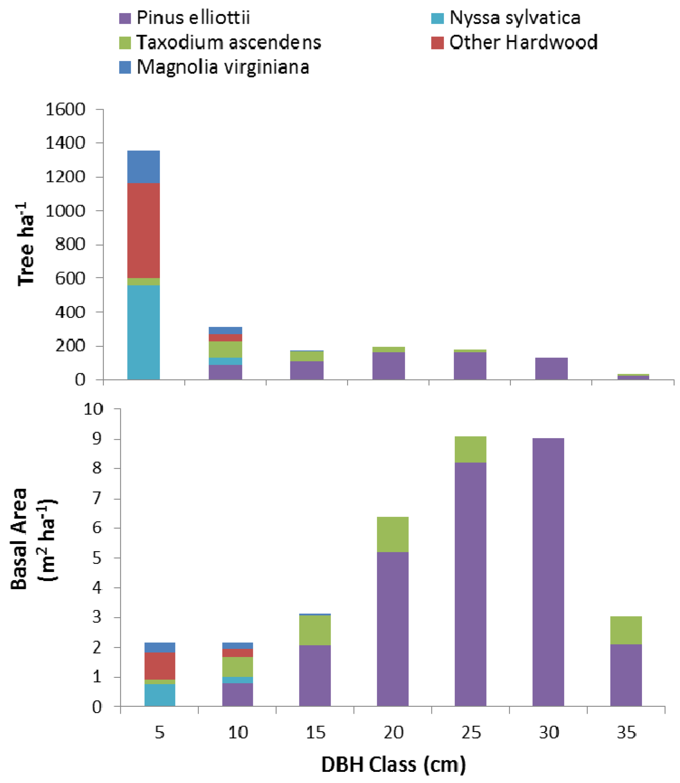
2.1. Simulation Input Data

We collected diameter at breast height (dbh) and species data for all the trees greater than 10 cm dbh from a 32-year-old unthinned slash pine plantation on a flatwoods site at Tate’s Hell State Forest, FL (29.83, −84.79) from five randomly established sample plots of 25 m × 25 m. Within the 25 m × 25 m plot, we measured all trees smaller than 10 cm dbh in two 5 m × 5 m plots at diagonally opposite corners. These data were input to FVS to initiate the growth simulation (Figure 1).

2.2. Model Description

We used FVS Model Version 1108—Southern U.S. PROGNOSIS RV: 11/20/13, developed by the USDA Forest Service (Fort Collins, CO, USA). FVS is a distance-independent, individual-tree forest growth model that uses individual stands as the basic units of projection. The required input key variables of each tree are its species and diameter, but information on height, crown ratio, diameter growth, and height growth may also be entered. The key variables for each sample point, or plot, include slope, elevation, aspect, density, and a measure of site potential. The self-calibration feature of FVS allows its internal growth models to adjust and match the measured growth rates of a particular location consistent with the source of the input data, thereby enabling the model to adapt to the local conditions [15,17].
FVS has the ability to simulate many types of harvest and other silvicultural activities, and can be applied to a variety of forest types and stand structures ranging from even-aged to uneven-aged and single to mixed species [15,17,18,19]. The user has the option to specify how many trees or the basal area from which size-classes should be retained at the end of any simulation cycle, along with other activities such as shrub removal or artificial planting. Typical growth and mortality rates are predicted as functions of postharvest conditions (residual densities/basal area, etc.). Broadly, the FVS model has four primary components: diameter growth, height growth, mortality, and crown change. Diameter growth, height growth, and crown change models are further divided into submodels that pertain to “small” trees (≤7.6 cm dbh) and those that pertain to “large” trees (≥7.6 cm dbh). The small tree growth relationships are driven by tree height from which diameter growth is then estimated. On the other hand, the large tree growth relationships are driven by diameter first, and then height growth is estimated from diameter growth and other tree and stand variables. The growth cycles in the simulator are set to 5- or 10-year time steps with up to 40 cycles allowed per simulation [15,17].
The southern variant of FVS, however, does not have a full regeneration model. The user must schedule regeneration (natural or planting) events by specifying input values for density and age and/or size of seedlings. The FVS model is widely used [10,20,21,22,23,24] and more details about its contents, description, structure, and applications can be found in Crookston and Dixon [15], Dixon [17], Donnelly et al. [18], Keyser [19], McGaughey [25], and van Dyck and Smith [26].
The inventory data collected from the slash pine plantation were used to initialize the simulations in FVS model using specific control variables (Table 1). Parameter inputs (e.g., location, ecological codes etc.) were selected which best represented the site conditions at our study area [19].
The outputs generated from FVS were used to calculate structural diversity, carbon stocks, and merchantable timber production as described in Section 2.4.

2.3. Description of Management Regimes

We simulated multiple even- and uneven-aged management scenarios representing alternative management regimes for pine flatwoods in Florida, as well as a no-action option.

2.3.1. Even-Aged Management Scenarios

A range of even-aged silvicultural regimes are currently practiced to manage pine stands in the southern United States that vary depending on species, management objectives, site conditions, planting densities, and desired rotation length among other factors [27]. For our study, we chose four different regimes of intensive plantation forestry practiced in the southern United States. In three of these even-aged scenarios, stands were established at initial planting densities of 1236 (Low Density, LD), 1780 (Moderate Density, MD) or 2224 (High Density, HD) seedlings per hectare. These three scenarios were then thinned at stand age of 20 years to residual basal areas of 16.1 m2·ha−1, clearcut at rotation of 35 years, and again planted the following year to repeat the rotation for the rest of the simulation period. These scenarios represented common regimes for multiple products (sawtimber and pulpwood) in southern pines. The fourth even-aged scenario represented an intensively managed pulpwood plantation (PP) regime. In this scenario, a stand was established at initial density of 2224 seedlings·ha−1 and clearcut at 25 years without any thinning, and again planted the next year to repeat the rotation for the duration of simulation period. We named these four scenarios EAM-LD (Even-Aged Management-Low Density), EAM-MD (Even-Aged Management-Medium Density), EAM-HD (Even-Aged Management-High Density), and EAM-PP (Even-Aged Management-Pulpwood Plantation), respectively (Table 2). All the scenarios were implemented following clearcutting of the existing mature stand.
We consider scenario EAM-MD to represent the most common even-aged management prescription followed by the state and other agencies and private landowners on slash pine flatwood sites where the input data were collected.

2.3.2. Uneven-Aged Management

There are numerous suggested methods to convert a plantation and manage it using uneven-aged silviculture [10,11,28,29]. We chose a strategy that involved implementing a “thinning from below” during the first cutting cycle, followed by thinning across diameter classes at the second cutting cycle, and then following with selection cuts (based on the BDq approach) from the third cutting cycle onwards [10] (Table 2). The uneven-aged stand under this scenario developed and maintained a typical reverse J-shaped diameter distribution [1,2] with residual basal area (B) of 11.5 m2·ha−1, a maximum dbh (D) of 61 cm, and q-factor of 1.4 for diameter class width of 5 cm. Cutting cycle harvests were scheduled every 10 years, with the first cut at the beginning of the simulation. For regeneration purposes, we assumed that 1250 slash pine seedlings of the average age of 3 years per hectare were regenerated 4 years following the harvest in each cutting cycle. In a previous study [10], we found that the slash pine stand structure and growth was not very sensitive to higher or lower regeneration levels compared to 1250 slash pine seedlings per hectare. In practice, pine regeneration, in both uneven-aged and even-aged stands, is often concurrent with considerable amounts of hardwoods and other competing vegetation that could limit regeneration survival without adequate site preparation. For modeling purposes, we assumed that the competing vegetation in the stands was kept under control using mechanical means, fire and/or herbicides.

2.3.3. No-Action

This scenario represented a case when the existing stand was allowed to grow without any silvicultural intervention during the simulation period. That is, no harvest or regeneration events were scheduled.
In all scenarios, simulation outputs included a tree list, a carbon report, a stand summary, and a cut list [17]. Individual trees in the tree list were then classified into diameter classes and height classes. We used a total of 14 diameter classes with class widths of 5.1 cm, ranging from size 0 (less than 2.54 cm) to 71.1+ cm (equal to or greater than 68.6 cm). For height, we used a total of 13 height classes with class widths of 3 m, ranging from 0 (less than 1.5 m) to 39.6+ m (equal to or greater than 38.1 m). In both the cases, the classes represented the mid points of the class widths.

2.4. Evaluation of Management Regimes

Each scenario was evaluated based on the resulting stand structural diversity, carbon stocks and merchantable timber.

2.4.1. Stand Structural Diversity

At every cycle of the simulation period, we calculated Shannon’s diversity index for both the diameter class and height class distributions with respect to the basal area constituted by them. Shannon’s index was calculated as equal to −∑pi ln pi, where “p” is the proportion of basal area constituted by a diameter class “i” [30]. Stand structural diversity was then obtained as the average of Shannon’s diversity index values for both diameter and height classes [10]. Values were plotted over time and the average of stand structural diversity values at all cycles during a simulation was calculated as average stand structural diversity under a given scenario. To estimate variability around the average stand structural diversity, we determined the coefficient of variation (CV) for each scenario.

2.4.2. Carbon Stock

The outputs of the carbon reports obtained from the model were grouped into aboveground stored carbon (consisting of aboveground live tree, standing dead trees, down dead wood, forest floor, and understory), belowground stored carbon (consisting of belowground live tree, and belowground dead tree), and total carbon removed in harvest at each year during the simulation period [31]. The total stand carbon at a given time was the sum of above and belowground stored carbon at that time. The following additional variables were calculated:
(a)
Total stand carbon at the beginning of the simulation (year 0) = Total aboveground stored carbon in year 0 + Total belowground stored carbon in year 0,
(b)
Total stand carbon at the end of the simulation (year 100) = Total aboveground stored carbon in year 100 + Total belowground stored carbon in year 100, and
(c)
Total additional carbon stored during the simulation period = (Total stand carbon at the end of simulation (year 100) + sum of carbon harvested during different cycles in simulation period) − Total stand carbon in the beginning of simulation (year 0).
Average annual carbon stock for each scenario was obtained by dividing the total additional carbon stored by 100.

2.4.3. Timber Production

From the FVS summary output generated in the simulations, we calculated values of the following variables:
(a)
Total merchantable timber produced during the simulation period = Total merchantable timber removed during simulation + Total merchantable timber left standing after year 100 − Total merchantable timber in year 0, and
(b)
Total sawtimber produced during the simulation period = Total sawtimber removed during simulation + Total sawtimber left standing after year 100 − Total sawtimber in year 0.
Average annual production of these variables was then obtained by dividing the totals by 100.

2.5. Statistical Analyses

As recommended by Hamilton [32] for the application of FVS, we ran 3 simulations for each scenario reseeding the random number generator. Means were then calculated for average annual values of stand structural diversity, carbon stocks, merchantable timber, and sawtimber for each scenario. Analyses of variance (ANOVA) were carried out and Tukey’s HSD (Honestly Significant Difference) test was performed at α = 0.05 to test for significant differences in the means for all the scenarios.

3. Results

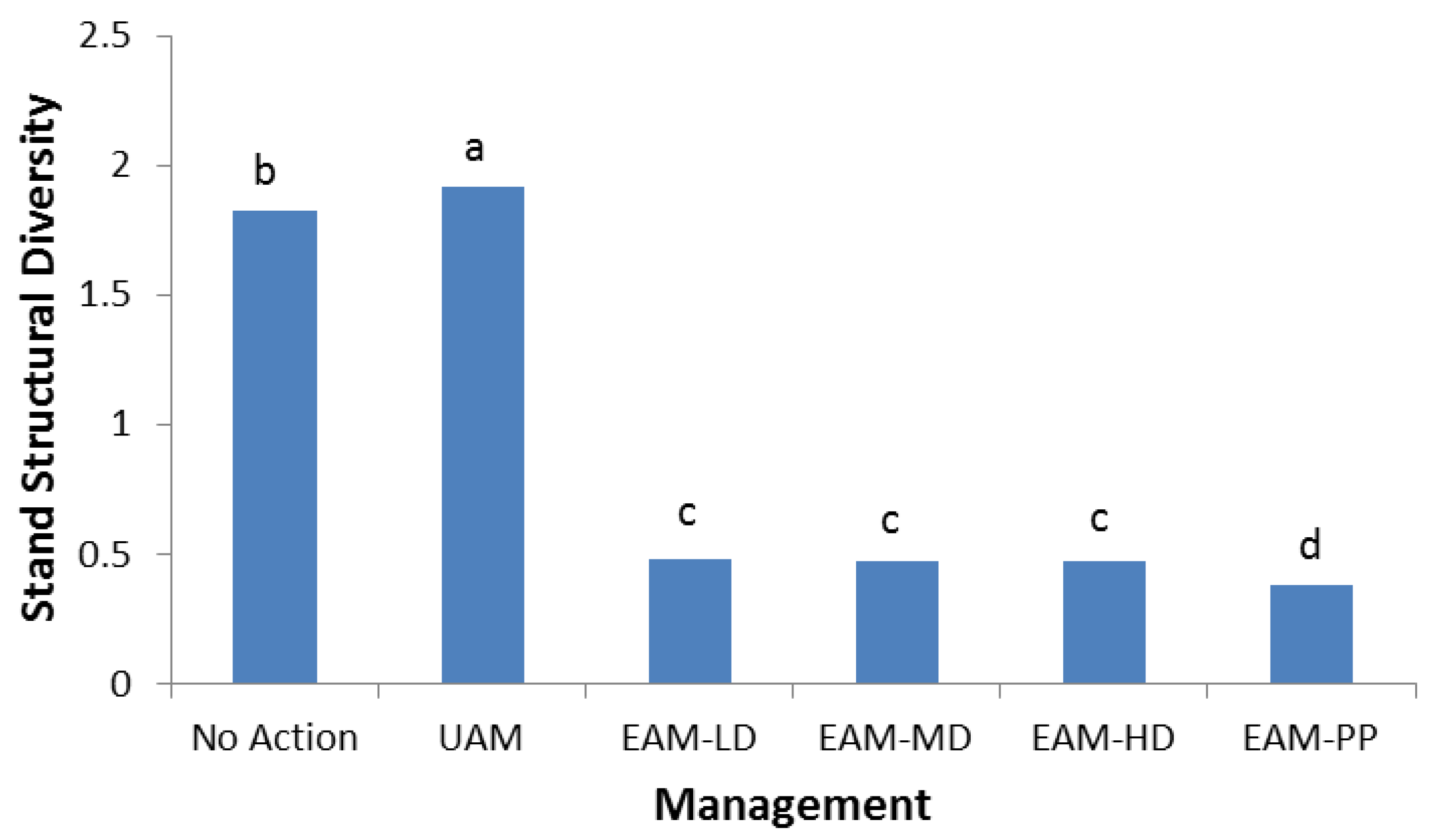
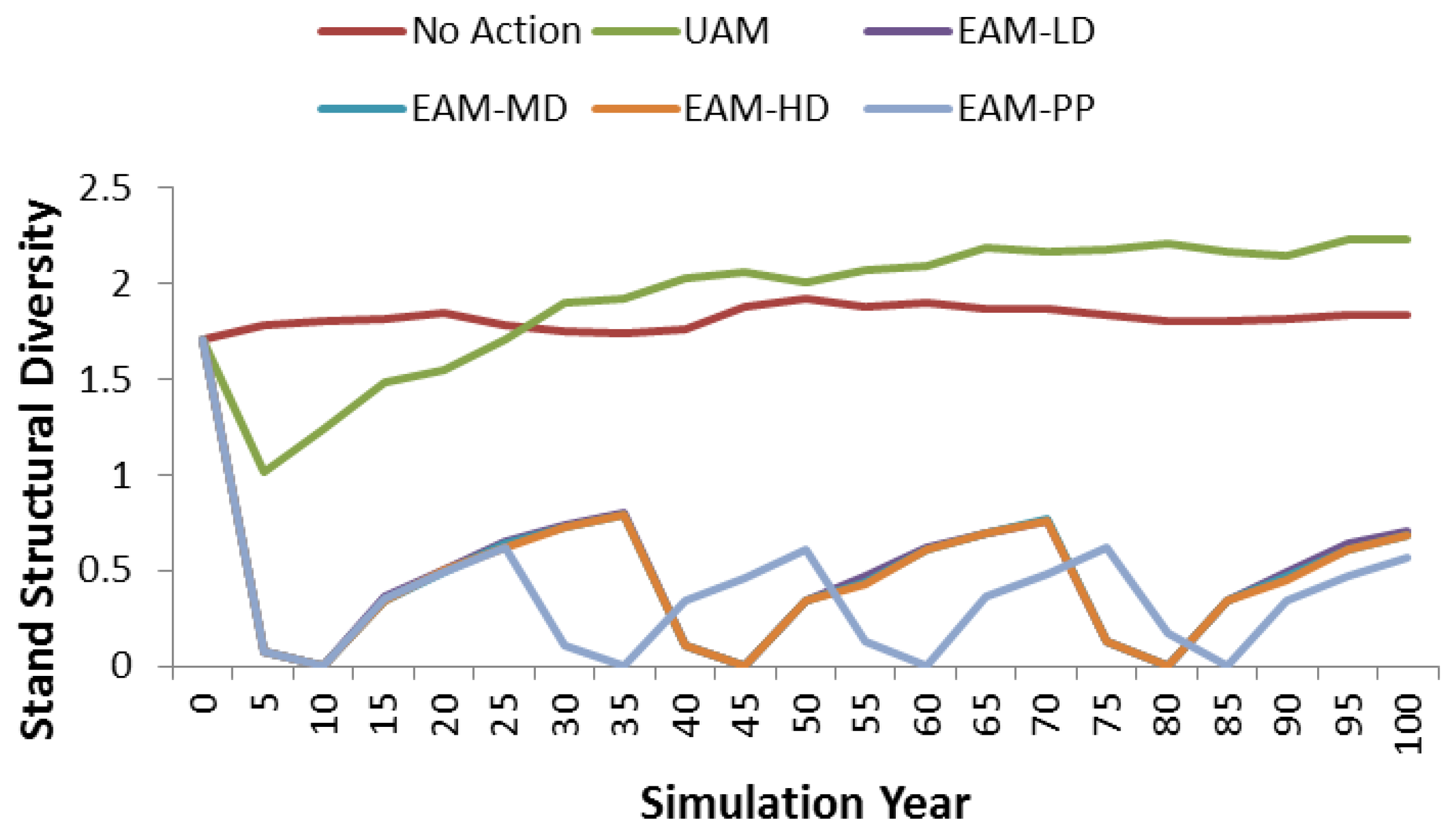
3.1. Stand Structural Diversity

Clear differences were found in the patterns of stand structural diversity among the scenarios. Uneven-aged management resulted in significantly higher stand structural diversity (1.92) than no-action (1.82) and even more so over all the even-aged scenarios averaged over the simulation period. Average stand structural diversity for even-aged management scenarios ranged from just 0.48 for EAM-LD and EAM-MD to 0.38 for EAM-PP. EAM-PP resulted in the least average stand structural diversity, significantly lower than other even-aged scenarios managed for multiple sawtimber-pulpwood products (Figure 2). The even-aged scenarios also resulted in substantially higher variability in stand structural diversity than those of uneven-aged or no-action scenarios over the simulation period. The pulpwood plantation regime (EAM-PP) resulted in the highest coefficient of variation (CV) of 100%, while uneven-aged and no-action scenarios had the lowest CVs of 17.9% and 3.0%, respectively. Other even-aged management scenarios EAM-LD, EAM-MD, and EAM-HD had CVs of 82.5%, 81.4%, and 82.7%, respectively.
Over the simulation period in the uneven-aged management scenario, stand structural diversity decreased from an initial value of 1.71 to 1.02 during the initial conversion period (thinning from below) that resulted in fewer size-classes in the residual stand. Later in the simulation, stand structural diversity increased gradually with minor fluctuations to surpass the initial level and reach a maximum of 2.27 at the end of 100 years (Figure 3). The no-action scenario more or less maintained, or slightly increased stand structural diversity. In the even-aged stands, dramatic fluctuations were evident in the patterns of structural diversity, which corresponded to the rotations (Figure 3). In EAM-MD, for example, the stand structural diversity dropped from the initial value of 1.71 to 0 as a clearcut was implemented and planting was done in the beginning years of the simulation. The stand then grew and differentiated into an increasing number of size classes resulting in a gradual increase in structural diversity from 0 to as much as 0.79 during a rotation before falling to 0 again at the beginning of next rotation. Even at its highest level, structural diversity in any even-aged management scenario at any time during the simulation period was never at the same level as that of the uneven-aged or no-action scenarios.

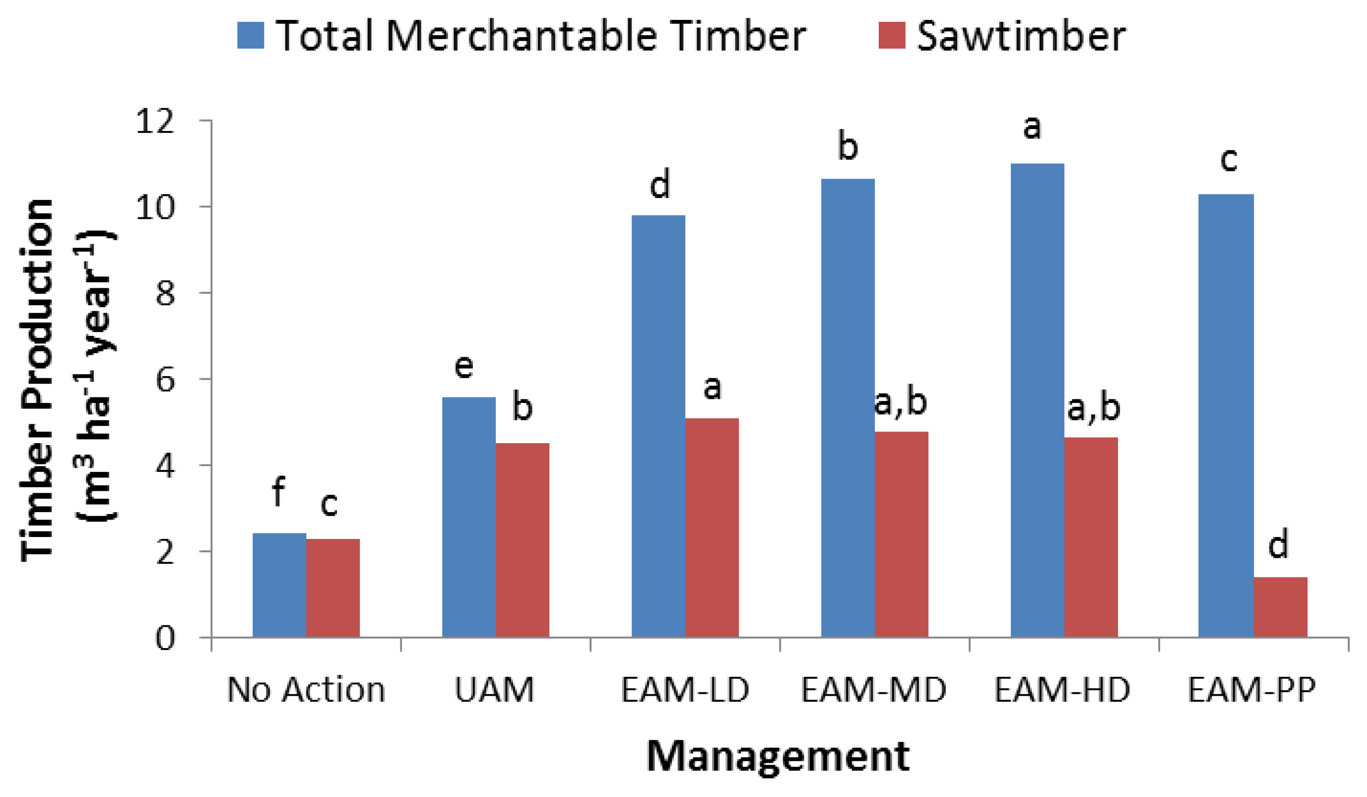
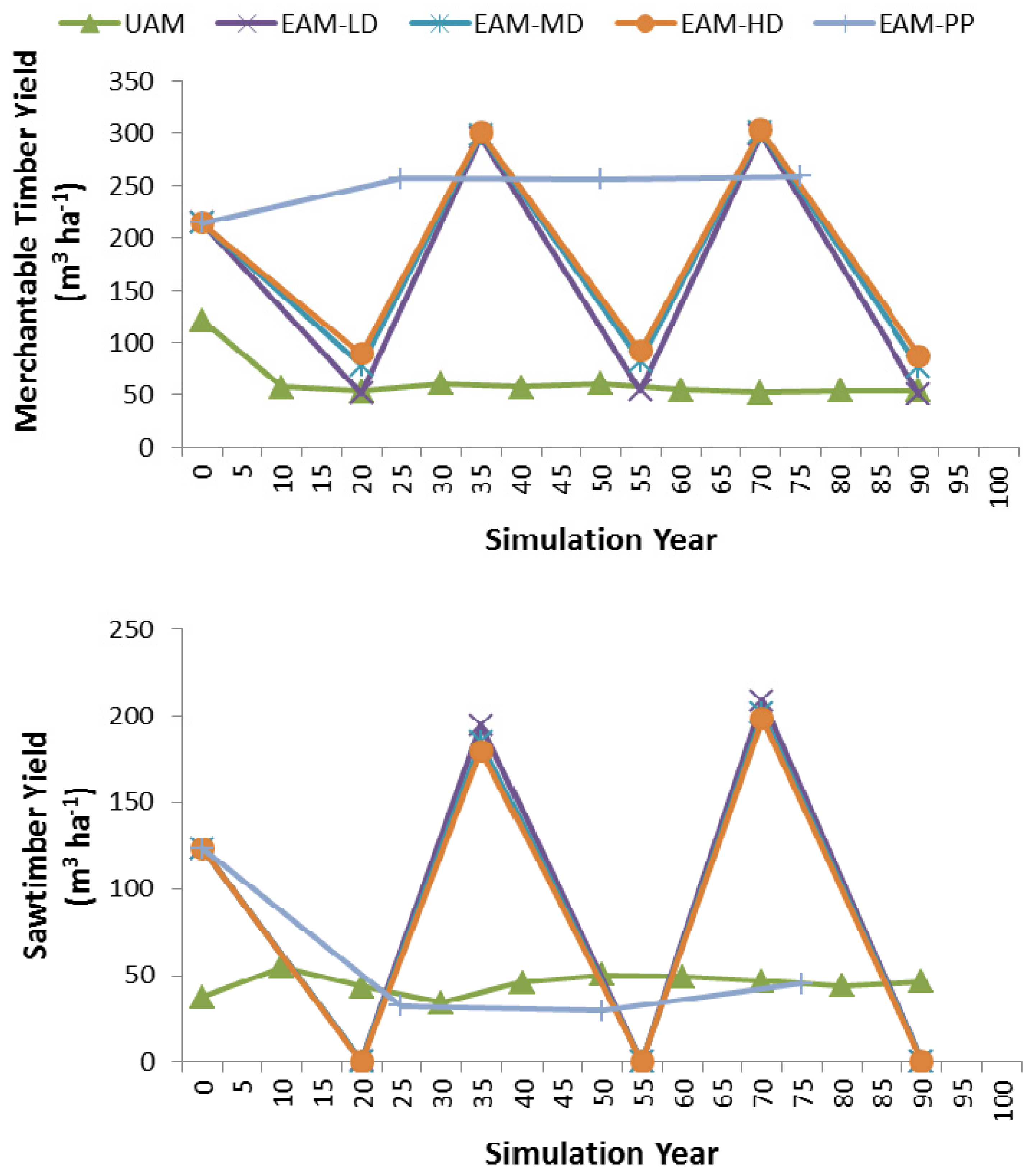
3.2. Timber Production
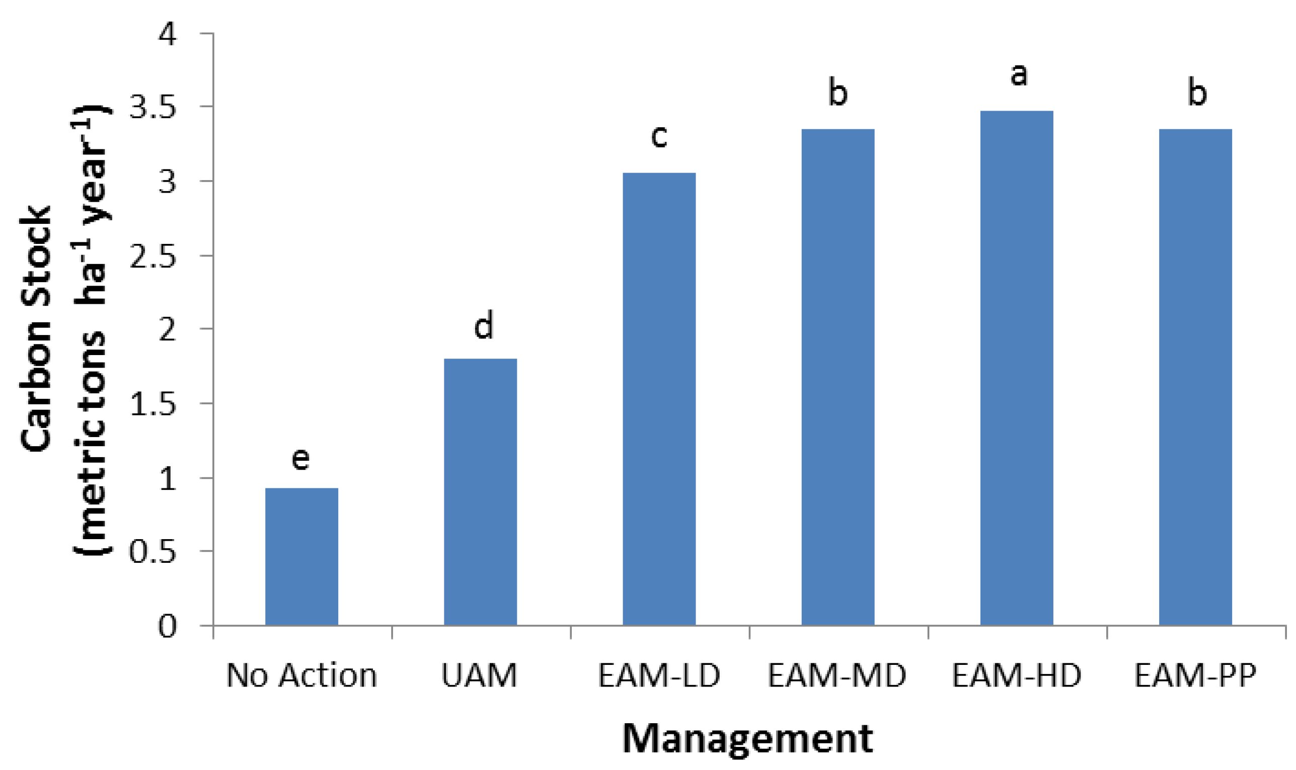
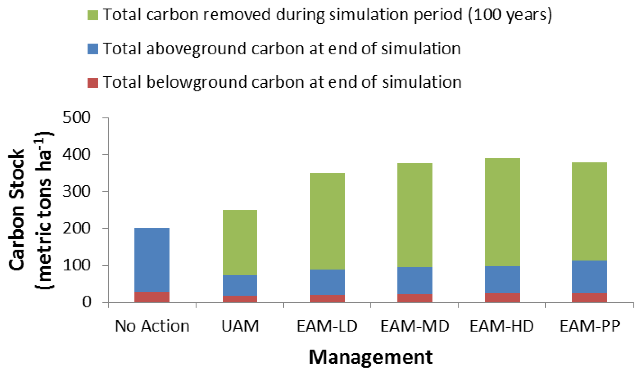
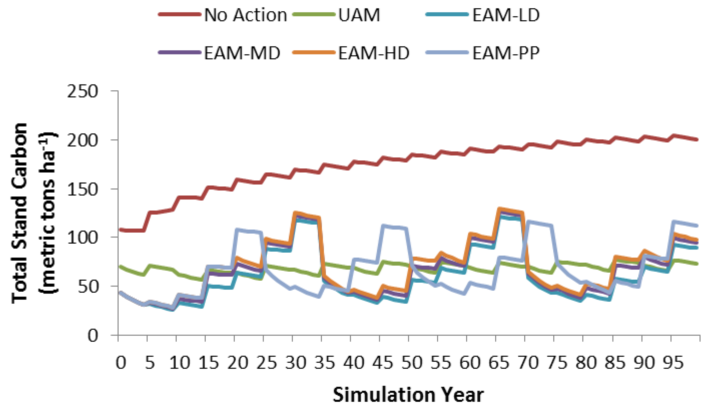
While all the scenarios significantly differed from one another in total merchantable timber production, all the even-aged management scenarios resulted in similar and significantly higher total merchantable timber production (9.78 to 11.02 m3·ha−1·year−1) than the uneven-aged management scenario (5.58 m3·ha−1·year−1), which, in turn, produced higher value than the no-action scenario (2.43 m3·ha−1·year−1) (Figure 4).
However, the pattern of sawtimber production across the scenarios differed from that of total merchantable production. Not surprisingly, in the EAM-PP scenario that represented a pulpwood plantation regime, the least amount of sawtimber (1.38 m3·ha−1·year−1) was produced. Uneven-aged management produced a similar amount of sawtimber as two of the even-aged scenarios (EAM-MD and EAM-HD), though just slightly lower than the even-aged scenario with the lower initial planting density (EAM-LD).
Yields obtained from thinning across the even-aged management scenarios (excluding EAM-PP) at 20 years into each rotation were between 50.03 and 91.99 m3·ha−1 and consisted of almost entirely (>98%) pulpwood, and yields obtained from clearcutting at the ends of rotations (35 years) over the simulation period consisted of approximately 30% to 40% pulpwood (88.70 to 119.77 m3·ha−1) and 60% to 70% sawtimber (179.92 to 209.03 m3·ha−1) (Figure 5). Pulpwood production regime (EAM-PP) resulted in 83% to 89% pulpwood (213.1 to 224.1 m3·ha−1) out of the total production (255.80 to 258.37 m3·ha−1) for each 25-year rotation.
Uneven-aged management, though not as productive overall in total merchantable production as even-aged management options, produced a steady and nearly similar output of sawtimber (34.29 to 54.86 m3·ha−1) compared to even-aged options. Sawtimber production during most cutting cycles constituted more than 80% of total merchantable timber (51.97 to 60.53 m3·ha−1) every 10 years. In the no-action scenario, growth added during the simulation period primarily led to increases in available sawtimber volume, although no yields were obtained as no harvests were carried out.

3.3. Carbon Stocks

Carbon stocks broadly followed the patterns of total merchantable timber in all scenarios, with all of the even-aged scenarios again resulting in significantly and substantially higher average annual carbon stocks (3.05 to 3.47 metric tons·ha−1·year−1) and the no-action scenario leading to the lowest quantity (0.93 metric tons·ha−1·year−1). Uneven-aged management resulted in moderate amounts of annual carbon stocks (1.80 metric tons·ha−1·year−1) (Figure 6).
About 70% of total carbon stocks consisted of the harvested timber in uneven-aged management and pulpwood production regime; this value increased to 75% in the rest of the even-aged scenarios (Figure 7). Not surprisingly, the no-action scenario in which no harvests were made consistently maintained the highest amounts of aboveground as well as belowground carbon stocks during the simulation period. Belowground carbon was the smallest constituent of total carbon stocks in all of the scenarios.
With regard to total standing carbon (aboveground plus belowground carbon in the stand at a given time excluding the harvested carbon), not surprisingly, the no-action scenario maintained gradually increasing amounts of total stand carbon that increased from 107.8 metric tons·ha−1 to 200.7 metric tons·ha−1 over 100 years (Figure 8). Uneven-aged management maintained steady carbon stocks ranging between 56.9 and 77.2 metric tons·ha−1. Even-aged management scenarios maintained carbon stocks that fluctuated widely between 25.9 and 129.9 metric tons·ha−1 over the simulation period. However, unlike timber production, carbon stocks in even-aged management scenarios never dropped to zero because of consistent belowground carbon stocks (Figure 8).

4. Discussion

4.1. Implications for Forest Management

Our study showed that even-aged management options were more efficient at total merchantable timber production while uneven-aged management created complex stand structure and maintained steady flow of yields, particularly sawtimber, and aboveground carbon stocks. Both even- and uneven-aged managements have the potential to improve production and carbon storage of pine forests and are substantial improvements over the no-action option.
Uneven-aged management resulted in higher average stand structural diversity and more consistent values over the simulation period than even-aged management. The structural diversity associated with uneven-aged stands is generally associated with enhancing species diversity and niche availability for both plant and animal species [33,34,35,36]. Maintaining consistent cover of large trees is also particularly important for some species, such as the threatened red-cockaded woodpecker (Picoides borealis Vieillot), which primarily utilizes longleaf pine species but will also nest in slash pine in hydric flatwoods [37]. Slash pine when managed using group selection system may also provide additional niche diversity by adding horizontally distributed, small even-aged gaps across the uneven-aged stand. On the other hand, in even-aged stands, greater variability in structure over time may provide for habitats to different species at different stages of stand development, particularly for those requiring early successional habitats [38,39].
As in our study, several studies on southern pines have also reported higher total timber production in even-aged stands [40,41,42]. Bragg and Guldin [43] simulated carbon sequestration in even- and uneven-aged loblolly and shortleaf pine dominated stands in the southern United States by accounting for live standing carbon as well as product pools with varying half-lives and reported that over a 100-year period the even-aged stands (naturally originated seed tree stand and short-rotation loblolly plantation) sequestered approximately 120 metric tons·ha−1 of carbon in live tree and product pools, or about 50% more than the uneven-aged stands. They also reported similar patterns of fluctuating aboveground biomass in even-aged stands and maintenance of steady aboveground carbon in uneven-aged stands as arose in our simulations. Averaged over the period, annual carbon sequestration in Bragg and Guldin [43] ranged from 0.38 to 1.11 to 1.16 metric tons·ha−1 for the uneven-aged, seed tree, and plantation, respectively. If Bragg and Guldin [43] considered only carbon accumulation via growth, and did not account for simultaneous losses (thus making their methods more similar to our methods), average annual carbon accumulation values of 0.81, 3.36, and 4.82 metric tons·ha−1·year−1 approximately were calculated for the uneven-aged stand, the seed tree stand, and the plantation in this study, respectively, which are comparable to the values generated in our simulation.
Carbon stocks and total timber production, although significantly higher under even-aged management scenarios, consisted of disproportionately higher amount of pulpwood as compared to those in uneven-aged management. This may be an important consideration because higher productivity or stored carbon does not necessarily infer higher long-term carbon benefits as carbon sequestration may depend on the end products (such as sawtimber or pulpwood derived products), which have varying half-lives [43]. Understandably, pulpwood will have a shorter half-life as compared to sawtimber [44]. Therefore, carbon benefits may not be proportional to the total timber production in each management scenario [45]. As such, it is possible that management of southern pines geared toward quality sawlog production may sequester more carbon over the long-term than short-rotation pulpwood plantations [43]. In our study, sawtimber production was just slightly higher in the even-aged scenario with low initial planting density than the uneven-aged scenario but was similar when initial planting density in even-aged scenarios increased to moderate and high levels on a 35 year rotation. When the rotation length was reduced and the planting density increased as in the pulpwood plantation scenario, sawtimber production was significantly reduced to the lowest level among all the scenarios, including the uneven-aged and the no action scenarios. The relative amount of sawtimber and pulpwood produced in a management system, therefore, can also have significant impact on the long-term carbon sequestration. Additionally, managing uneven-aged stands on a more irregular basis with longer cutting cycles, as we found in Sharma et al. [10] and other studies [43,46], may also result in carbon accumulation similar or higher to those in even-aged stands.
Although we did not do any economic analysis, several other studies have compared these two management alternatives, albeit primarily focused on timber. While Cafferata and Kemperer [47] and Axelsson and Angelstam [48] reported even-aged management to be financially superior, some other comprehensive studies [3,9,33,49,50,51,52,53] have found uneven-aged stands to be equally or more financially attractive. Uneven-aged management, unlike even-aged management, also offers the opportunity of regular, continuous income from the southern pine forests [9]. However, even-aged plantation forestry offers the potential to significantly increase productivity over time through the use of improved genetic material, seedling production technology, site preparation, and other intensive operations such as fertilization and vegetation control, which would lead to increased financial returns over time [54]. While some suggest that these advantages will result in increased timber productivity on a smaller land-base, others still have concern about the potential ecological impacts of intensive plantation management if used solely for financial objectives, particularly since wide-scale land-use change from natural forests to forest plantations has resulted in significant loss of biodiversity and habitat in the past [55].
Our study has shown the tradeoffs of forest structure and productivity for alternative management systems for southern pine forests. None of the management scenarios will maximize production, carbon storage and structural complexity simultaneously. The projected increase in population and demand for diverse forest products and services in the southern United States may not be met with any single management system dominating over vast expanses of regional landscapes. Therefore, optimal achievement of multiple benefits may require maintaining an assortment of alternative management strategies over the landscape [4]. Other management options may include a compromise between the two alternatives in which the land managers may devise strategies that maintain uneven-aged stands with a little longer cutting cycle to balance the objectives of production and carbon storage along with services associated with complex forest structure.

4.2. Limitations of the Study

This study used a simple set of the alternative even- and uneven-aged management options to evaluate outcomes for a southern pine species. In practice, management regimes would be complex and highly variable involving different combinations of cutting cycles or rotations and residual basal areas along with many confounding factors or additional intensive operations like fertilization, herb and shrub control, etc. Fire, which is an important ecological disturbance as well as management tool in these ecosystems, was also not modeled. A number of other factors related to management such as continuously improving genetic stock of artificially regenerated slash pine, or changing climatic conditions, which could lead to stochastic events such as hurricane-induced mortality, etc., have the potential to drastically affect the performances of the management options. FVS carbon reporting also did not include carbon fluxes such as management related emissions (e.g., carbon emitted from equipment use when harvesting and transporting timber, transporting nursery stock for planting, etc.). A complete carbon footprint analysis would include life-cycle assessment of all aspects of forest management, such as the emissions associated with the production, transportation, and application of fertilizers [31]. Economic analyses in terms of costs and benefits of activities and products in different management scenarios will have a huge impact in management decision-making.

5. Conclusions

The challenge to forest management on many lands is to optimize the provision of both commodity and non-commodity services. No single management alternative will lead to maximization of all products and services. There are always tradeoffs involved. While even-aged systems will tend to maximize total merchantable timber production, uneven-aged systems will maximize structural diversity and related ecosystem services requiring such diversity. Uneven-aged management also produces sawtimber and carbon stocks comparable to even-aged management, on a shorter and more regular interval. Thus, uneven-aged management of forest may represent a good balance of meeting multiple objectives for environmental services and habitats as well as sawtimber on a stand level, while even-aged management may be preferred by land managers when a high amount of timber and primarily pulpwood production is of paramount importance. On a landscape scale, optimal achievement of multiple benefits may require maintaining an assortment of management strategies.

Acknowledgments

This work was supported by the cooperative for Conserved Forest Ecosystems—Outreach and Research (CFEOR) and the USDA National Institute of Food and Agriculture, Evans–Allen project #1006138. The authors gratefully acknowledge the efforts of Michael Morgan, Melissa Kreye, Justin McKeithen, Pritika Sharma, Dhiraj Vyas, and others, for helping with the fieldwork, and David Morse and the Florida Forest Service for the opportunity to use the state forestlands.

Author Contributions

All the authors (A.S., K.B., S.J. and P.D.) conceived the idea of study and designed the methodology; A.S. and K.B. performed the simulations; A.S. K.B. and P.D. analyzed the data; K.B. and S.J. contributed materials and analysis tools; A.S., K.B., S.J. and P.D. all contributed to writing the paper.

Conflicts of Interest

The authors declare no conflict of interest. The founding sponsors had no role in the design of the study, in the collection, analyses, or interpretation of data, in the writing of the manuscript, and in the decision to publish the results.

References

  1. Smith, D.M.; Larson, B.C.; Kelty, M.J.; Ashton, P.M.S. The Practice of Silviculture: Applied Forest Ecology; John Wiley and Sons: New York, NY, USA, 1997; p. 537. [Google Scholar]
  2. Nyland, R.D. Silviculture: Concepts and Applications, 2nd ed.; McGraw-Hill: New York, NY, USA, 2002; p. 682. [Google Scholar]
  3. O’Hara, K.L.; Nagel, L.M. A functional comparison of productivity in even-aged and multi-aged stands: A synthesis for Pinus ponderosa. For. Sci. 2006, 52, 290–303. [Google Scholar]
  4. O’Hara, K.L. Multiaged Silviculture: Managing for Complex Stand Structures; Oxford University Press: Oxford, UK, 2014; p. 213. [Google Scholar]
  5. Puettmann, K.J.; Wilson, S.M.; Baker, S.C.; Donoso, P.J.; Drössler, L.; Amente, G.; Harvey, B.D.; Knoke, T.; Lu, Y.; Nocentini, S.; et al. Silvicultural alternatives to conventional even-aged forest management—What limits global adoption. For. Ecosyst. 2015, 2, 1–16. [Google Scholar] [CrossRef]
  6. Guldin, J.M. Experience with the selection method in pine stands in the southern United States, with implications for future application. Forestry 2011, 84, 539–546. [Google Scholar] [CrossRef]
  7. Wear, D.N.; Greis, J.G. The Southern Forest Futures Project: Summary Report; General Technical Report SRS-168; U.S. Department of Agriculture Forest Service, Southern Research Station: Asheville, NC, USA, 2012. [Google Scholar]
  8. Huggett, R.; Wear, D.N.; Li, R.; Coulston, J.; Liu, S. Forecasts of Forest Conditions. In The Southern Forest Futures Project: Technical Report; General Technical Report SRS-GTR-178; Wear, D.N., Greis, J.G., Eds.; USDA-Forest Service, Southern Research Station: Asheville, NC, USA, 2013; pp. 73–102. [Google Scholar]
  9. Handley, D.M.; Dickinson, J.C. A better way—Uneven-aged management of southern yellow pine. In Proceedings of the 15th Biennial Southern Silvicultural Research Conference, General Technical Report SRS-GTR-175, Hot Springs, AR, USA, 17–20 November 2008; Guldin, J.M., Ed.; U.S. Department of Agriculture, Forest Service, Southern Research Station: Asheville, NC, USA, 2013; pp. 39–43. [Google Scholar]
  10. Sharma, A.; Bohn, K.K.; Jose, S.; Cropper, W.P., Jr. Converting even-aged plantations to uneven-aged stand conditions: A simulation analysis of silvicultural regimes with slash pine (Pinus elliottii Engelm.). For. Sci. 2014, 60, 893–906. [Google Scholar] [CrossRef]
  11. Loewenstein, E.F. Conversion of uniform broadleaved stands to an uneven-aged structure. For. Ecol. Manag. 2005, 215, 103–112. [Google Scholar] [CrossRef]
  12. Florida Division of Forestry. Ten-Year Resource Management Plan for the Tate’s Hell State Forest, Franklin and Liberty Counties; Florida Division of Agriculture and Consumer Services, Division of Forestry: Carrabelle, FL, USA, 2007; p. 73. [Google Scholar]
  13. Vanclay, J.K. Modelling Forest Growth and Yield: Applications to Mixed Tropical Forests; CAB International: Wallingford, UK, 1994; p. 312. [Google Scholar]
  14. Haefner, J.W. Modeling Biological Systems. Principles and Applications, 2nd ed.; Springer: New York, NY, USA, 2005; p. 473. [Google Scholar]
  15. Crookston, N.L.; Dixon, G.E. The forest vegetation simulator: A review of its structure, content, and applications. Comput. Electron. Agric. 2005, 49, 60–80. [Google Scholar] [CrossRef]
  16. Smith, W.; Miles, P.; Perry, C.; Pugh, S. Forest Resources of the United States, 2007: A Technical Document Supporting the Forest Service 2010 RPA Assessment. Available online: http://www.fs.fed.us/nrs/pubs/gtr/gtr_wo78.pdf (accessed on 5 February 2016).
  17. Dixon, G.E. Essential FVS: A User’s Guide to the Forest Vegetation Simulator; Internal Report; USDA Forest Service, Forest Management Service Center: Fort Collins, CO, USA, 2002; p. 226. [Google Scholar]
  18. Donnelly, D.; Lilly, B.; Smith, E. The Southern Variant of the Forest Vegetation Simulator; USDA Forest Service, Forest Management Service Center: Fort Collins, CO, USA, 2001; p. 61. [Google Scholar]
  19. Keyser, C.E. Southern (SN) Variant Overview—Forest Vegetation Simulator; Internal Report; USDA Forest Service, Forest Management Service Center: Fort Collins, CO, USA, 2008; p. 80. [Google Scholar]
  20. Teck, R.; Moeur, M.; Eav, B. Forecasting ecosystems with the Forest Vegetation Simulator. J. For. 1996, 94, 7–10. [Google Scholar]
  21. Gilmore, D.W. To thin or not to thin: Using the Forest Vegetation Simulator to evaluate thinning of aspen. North. J. App. For. 2003, 20, 14–18. [Google Scholar]
  22. Johnson, M.C.; Peterson, D.L.; Raymond, C.L. Guide to Fuel Treatments in Dry Forests of the Western United States: Assessing Forest Structure and Fire Hazard; U.S. Department of Agriculture, Forest Service, Pacific Northwest Research Station: Portland, OR, USA, 2007; p. 322. [Google Scholar]
  23. Sorensen, D.C.; Finkral, J.A.; Kolb, E.T.; Huang, H.C. Short and long term effects of thinning and prescribed fire on carbon stocks in ponderosa pine stands in northern Arizona. For. Ecol. Manag. 2011, 261, 460–472. [Google Scholar] [CrossRef]
  24. Saunders, M.R.; Arseneault, J.E. Potential yields and economic returns of natural disturbance-based silviculture: A case study from the Acadian Forest Ecosystem Research Program. J. For. 2013, 111, 175–185. [Google Scholar] [CrossRef]
  25. McGaughey, R.J. Visualizing forest stand dynamics using the stand visualization system. In Proceedings of the 1997 ACSM-ASPRS Annual Convention and Exposition, Seattle, WA, USA, 7–10 April 1997; American Society of Photogrammetry and Remote Sensing: Bethesda, MD, USA, 1997; Volume 4, pp. 248–257. [Google Scholar]
  26. Van Dyck, M.G.; Smith, E.E. Keyword Reference Guide for the Forest Vegetation Simulator; Internal Report; U.S. Department of Agriculture, Forest Service, Forest Management Service Center: Fort Collins, CO, USA, 2000; p. 122. [Google Scholar]
  27. Dickens, E.D.; Will, R.E. Planting density impacts on slash pine stand growth, yield, product class distribution, and economics. In Slash Pine: Still Growing and Growing, Proceedings of the Slash Pine Symposium, General Technical Report SRS-76, Jekyll Island, GA, USA, 23–25 April 2002; Dickens, E.D., Barnett, J.P., Hubbard, W.G., Jokela, E.J., Eds.; USDA Forest Service Southern Research Station: Asheville, NC., USA, 2004; pp. 36–44. [Google Scholar]
  28. Nyland, R.D. Even- to uneven-aged: The challenges of conversion. For. Ecol. Manag. 2003, 172, 291–300. [Google Scholar] [CrossRef]
  29. Loewenstein, E.F.; Guldin, J.M. Conversion of Successionally Stable Even-Aged Oak Stands to an Uneven-Aged Structure. 2004. Available online: http://www.srs.fs.usda.gov/pubs/gtr/gtr_srs073/gtr_srs073-loewenstein001.pdf (accessed on 5 February 2016). [Google Scholar]
  30. Magurran, A.E. Ecological Diversity and Its Measurement; Princeton University Press: Princeton, NJ, USA, 1988; p. 192. [Google Scholar]
  31. Hoover, C.M.; Rebain, S.A. Forest Carbon Estimation Using the Forest Vegetation Simulator: Seven Things You Need to Know. 2011. Available online: http://www.nrs.fs.fed.us/pubs/gtr/gtr_nrs77.pdf (accessed on 5 February 2016).
  32. Hamilton, D.A. Implications of Random Variation in the Stand Prognosis Model. 1991. Available online: http://www.treesearch.fs.fed.us/pubs/8963 (accessed on 5 February 2016).
  33. Pukkala, T.; Lahde, E.; Laiho, O.; Salo, K.; Hotanen, J. A multifunctional comparison of even-aged and uneven-aged forest management in a boreal region. Can. J. For. Res. 2011, 41, 851–862. [Google Scholar] [CrossRef]
  34. MacArthur, R.H.; MacArthur, J.W. On bird species diversity. Ecology 1961, 42, 594–598. [Google Scholar] [CrossRef]
  35. Jalonen, J.; Vanha-Majamaa, I. Immediate effects of four different felling methods on mature boreal spruce forest understorey vegetation in southern Finland. For. Ecol. Manag. 2001, 146, 25–34. [Google Scholar] [CrossRef]
  36. Matveinen-Huju, K.; Koivula, M. Effects of alternative harvesting methods on boreal forest spider assemblages. Can. J. For. Res. 2008, 38, 782–794. [Google Scholar] [CrossRef]
  37. Porter, M.L.; Labisky, R.L. Home range and foraging habitat of red-cockaded woodpeckers in northern Florida. J. Wildl. Manag. 1986, 50, 239–247. [Google Scholar] [CrossRef]
  38. Owens, F.L.; Stouffer, P.C.; Chamberlain, M.J.; Miller, D.A. Early-successional breeding bird communities in intensively managed pine plantations: Influence of vegetation succession but not site preparations. Southeast. Nat. 2014, 13, 423–443. [Google Scholar] [CrossRef]
  39. Johnson, A.S.; Landers, J.L. Habitat relationships of summer resident birds in slash pine flatwoods. J. Wildl. Manag. 1982, 46, 416–428. [Google Scholar] [CrossRef]
  40. Williston, H.L. Uneven-aged management in the loblolly-shortleaf pine forest type. South. J. Appl. For. 1978, 2, 78–82. [Google Scholar]
  41. Guldin, J.M.; Baker, J.B. Yield comparisons from even-aged and uneven-aged loblolly-shortleaf pine stands. South. J. Appl. For. 1988, 12, 107–114. [Google Scholar]
  42. Cain, M.D.; Shelton, M.G. Natural loblolly and shortleaf pine productivity through 53 years of management under four reproduction cutting methods. South. J. Appl. For. 2001, 25, 7–16. [Google Scholar]
  43. Bragg, D.C.; Guldin, J.M. Estimating long-term carbon sequestration patterns in even- and uneven-aged southern pine stands. In Integrated Management of Carbon Sequestration And Biomass Utilization Opportunities in a Changing Climate, Proceedings of the 2009 National Silviculture Workshop, Boise, ID, USA, 15–18 June 2009; Jain, T.B., Graham, R.T., Sandquist, J., Eds.; Department of Agriculture, Forest Service, Rocky Mountain Research Station: Fort Collins, CO, USA, 2010. [Google Scholar]
  44. Birdsey, R.A. Carbon storage for major forest types and regions in the conterminous United States. In Forests and Global Change, Volume Two—Forest Management Opportunities for Mitigating Carbon Emissions; Sampson, R.N., Hair, D., Eds.; American Forests: Washington, DC, USA, 1996; pp. 1–25. [Google Scholar]
  45. Dwivedi, P.; Khanna, M.; Sharma, A.; Susaeta, A. Efficacy of carbon and bioenergy markets in mitigating carbon emissions on reforested lands: A case study from Southern United States. For. Pol. Econ. 2016, 67, 1–9. [Google Scholar] [CrossRef]
  46. Dwivedi, P.; Bailis, R.; Khanna, M. Is use of both pulpwood and logging residues instead of only logging residues for bioenergy development a viable carbon mitigation strategy? Bioenergy Res. 2014, 7, 217–231. [Google Scholar] [CrossRef]
  47. Cafferata, M.J.S.; Kemperer, W.D. Economic Comparisons between Even-Aged and Uneven-Aged Loblolly Pine Silvicultural Systems; Technical Bulletin No. 801; National Council for Air and Stream Improvement, Inc. Research: Triangle Park, NC., USA, 2000. [Google Scholar]
  48. Axelsson, R.; Angelstam, P. Uneven-aged forest management in boreal Sweden: Local forestry stakeholders’ perceptions of different sustainability dimensions. Forestry 2011, 84, 567–579. [Google Scholar] [CrossRef]
  49. Haight, R.G. Evaluating the efficiency of even-aged and uneven-aged stand management. For. Sci. 1987, 33, 116–134. [Google Scholar]
  50. Tarp, P.; Buongiorno, J.; Helles, F.; Larsen, J.B.; Meilby, H.; Strange, N. Economics of converting an even-aged Fagus sylvatica stand to an uneven-aged stand using target diameter harvesting. Scand. J. For. Res. 2005, 20, 63–74. [Google Scholar] [CrossRef]
  51. Tahvonen, O.; Pukkala, T.; Laiho, O.; Lahde, E.; Niinimaki, S. Optimal management of uneven-aged Norway spruce stands. For. Ecol. Manag. 2010, 260, 106–115. [Google Scholar] [CrossRef]
  52. Kuuluvainen, T.; Tahvonen, O.; Aakala, T. Even-aged and uneven-aged forest management in boreal Fennoscandia: A review. Ambio 2012, 41, 720–737. [Google Scholar] [CrossRef] [PubMed]
  53. Laiho, O.; Lahde, E.; Pukkala, T. Uneven- vs. even-aged management in Finnish boreal forests. Forestry 2011, 84, 547–556. [Google Scholar] [CrossRef]
  54. Fox, T.R.; Jokela, E.J.; Allen, H.L. The development of pine plantation silviculture in the southern United States. J. For. 2007, 105, 337–347. [Google Scholar]
  55. Wear, D.; Abt, R.; Alavalapati, J.; Comatas, G.; Countess, M.; McDow, W. The South’s Outlook for Sustainable Forest Bioenergy and Biofuels Production. The Pinchot Institute Report. 2010. Available online: http://www.srs.fs.fed.us/pubs/ja/2010/ja_2010_wear_001.pdf (accessed on 5 February 2016).
Figure 1. Inventory stand data input to Forest Vegetation Simulator to simulate alternative management regimes in managing slash pine (Pinus elliottii Engelm.). Dense stand conditions and absence of any hardwood control measures in the past few years had resulted in dense shrubby undergrowth. A few large overstory hardwood trees left uncut at the end of last rotation also existed. Stand basal area was approximately 35 ± 3.7 m2·ha−1.
Forests 07 00086 g001
Figure 2. Stand structural diversity (average Shannon’s index value) under alternative management scenarios for slash pine, averaged over a 100-year simulation period. The values of stand structural diversity with the same letter did not differ significantly.
Forests 07 00086 g002
Figure 3. Temporal dynamics of stand structural diversity during the 100-year simulation period under alternative management scenarios for slash pine.
Forests 07 00086 g003
Figure 4. Timber production under alternative management scenarios for slash pine. Values with different letters within each of the two variables differed significantly from each other.
Forests 07 00086 g004
Figure 5. Timber yields at multiple cutting cycles during the 100-year simulation period under alternative management scenarios for slash pine. The “No Action” scenario in which no harvest was carried out did not yield (remove) any timber during the simulation period.
Forests 07 00086 g005
Figure 6. Total carbon stock added annually in alternative management scenarios for slash pine. The values of carbon stock with the same letter did not differ significantly.
Forests 07 00086 g006
Figure 7. Total carbon (standing + harvested during the simulation period) under alternative management regimes for slash pine.
Forests 07 00086 g007
Figure 8. Temporal dynamics of total stand carbon (aboveground and belowground) during the 100-year simulation period under alternative management scenarios for slash pine.
Forests 07 00086 g008
Table 1. Control variables inputs specified to FVS-southern variant to control the simulation for the study.
Parameter or AttributeInput Setting
Location Code80501 (Apalachicola National Forest in Florida, Latitude: 30.44 N, Longitude: 84.28 W)
Ecological Unit codes232Dd (Gulf coastal lowlands)
Slope (%)0
Aspect0
Elevation(m)9.15
Site Species Codes (Alpha code)SA, PC, MV,OH, WT
Site Index(m) for slash pine25.91
Number of projection cycles20
Projection cycle length5
Volume equationsNational Volume Estimator Library
Volume Specifications:
Minimum Diameter at Breast Height/Top Diameter InsidePulpwoodSawtimber
Bark (cm)
Stump Height (cm)
10.2/10.2
30.5
25.4/17.8
30.5
Sampling Design
Large trees (fixed area plot)−6.5
Small trees (fixed area plot)81
Breakpoint Diameter at Breast Height (cm) 110.2
1 Trees equal to or larger than the breakpoint diameter were measured in large fixed area plots (25 m × 25 m), and trees with diameters below the breakpoint were measured in two small fixed area plots (5 m × 5 m each) within the large plots.
Table 2. Scenarios representing common even- and uneven-aged silvicultural regimes for slash pine in flatwood sites as simulated in the study.
Scenarios 1
No ActionUAMEAM-LDEAM-MDEAM-HDEAM-PP
DescriptionNo silvicultural interventionUneven-aged management Even-aged management with low initial planting densityEven-aged management with moderate initial planting densityEven-aged management—high initial planting densityEven-aged management forpulpwood production with high initial planting density and no thinning.
Residual Basal Área (B) (m2·ha−1)NA 2Low thinning (seed cut) at first cutting cycle reducing basal area to 11.5 m2·ha−1; Second cutting cycle (thinning across the diameter classes) and successive cutting cycles implementing BDq cut reducing basal area to 11.5 m2·ha−116.1 m2·ha−116.1 m2·ha−116.1 m2·ha−1NA
Maximum Diameter (D) (cm)NA>61NANANANA
Diminution Quotient (q)NA1.4NANANANA
Cutting Cycle (years)NA10NANANANA
Rotation (years)NANA35353525
ThinningsNANAThird row thin at 20 year, reducing basal area to 16.1 m2·ha−1Same as EAM-LDSame as EAM-LDNone
Regeneration 3 (seedlings/ha)NA12501236178022242224
1 UAM, Uneven-Aged Management; EAM-LD, Even-Aged Management-Low Density; EAM-MD, Even-Aged Management-Medium Density; EAM-HD, Even-Aged Management-High Density; and EAM-PP, Even-Aged Management-Pulpwood Plantation; 2 Not Applicable; 3 Regeneration was input in Forest Vegetation Simulator’s partial regeneration establishment extension as number of seedlings of (a) average age of four years observed four years after clearcuts in even aged scenario; and (b) average age of three years observed after four years of regeneration cuttings in each cutting cycle for uneven-aged scenario.

