Time-Lag Effect of Climate Conditions on Vegetation Productivity in a Temperate Forest–Grassland Ecotone

Abstract

Climate conditions can significantly alter the vegetation net primary productivity (NPP) in many of Earth’s ecosystems, although specifics of NPP–climate condition interactions, especially time-lag responses on seasonal scales, remain unclear in ecologically sensitive forest–grassland ecotones. Based on the Moderate-Resolution Imaging Spectroradiometer (MODIS) and meteorological datasets, we analyzed the relationship between NPP and precipitation, temperature, and drought during the growing season (April–August), considering the time-lag effect (0–5 months) at the seasonal scale in Hulunbuir, Inner Mongolia, China from 2000 to 2018. The results revealed a delayed NPP response to precipitation and drought throughout the growing season. In April, the precipitation in the 4 months before (i.e., the winter of the previous year) explained the variation in NPP. In August, the NPP in some areas was influenced by the preceding 1~2 months of drought. The time-lag effect varied with vegetation type and soil texture at different spatial patterns. Compared to grass and crop, broadleaf forest and meadow exhibited a longer legacy of precipitation during the growing season. The length of the time-lag effects of drought on NPP increased with increasing soil clay content during the growing season. The interaction of vegetation types and soil textures can explain 37% of the change in the time-lag effect of the NPP response to PPT on spatial pattern. Our findings suggested that preceding precipitation influences vegetation growth at the early stages of growth, while preceding drought influences vegetation growth in the later stages of growth. The spatial pattern of the time lag was significantly influenced by interaction between vegetation type and soil texture factors. This study highlights the importance of considering the time-lag effects of climate conditions and underlying drivers in further improving the prediction accuracy of NPP and carbon sinks in temperate semiarid forest–grassland ecotones.

1. Introduction

Climate change increases the severity and frequency of extreme events, which are expected to further affect ecosystem structure and functioning profoundly [1,2,3] and alter hydrothermal conditions in many regions worldwide, consequently influencing vegetation productivity [4,5]. Net primary productivity (NPP) has become an indispensable index used for ecosystem response measurement and quantitative analysis carbon budgets under climate change [5,6,7,8].

Many researchers have analyzed the relationship between NPP and climate conditions and have found that NPP responses to climate conditions exhibit a certain time lag [2,9,10,11]. Other researchers have found that, regarding time-lag effects, climatic factors can explain 64% of the variation in global plant growth and vegetation dynamics, which is 11% higher than model results ignoring time-lag effects [12]. However, most current studies consider only the time-lag effect on an annual scale or throughout the entire growing season [13], but the occurrence and length of the time-lag effect at different vegetation growth stages remain unclear. Compared to the entire growing season, the vegetation growth response to climate conditions can vary between different growth stages, as the various vegetation growth stages differ in water, energy, and nutrient requirements [14]. For example, the previous year’s autumn and winter precipitation has a negative effect on the spring leaf unfolding, and early spring precipitation has a positive effect. The main factor limiting vegetation development in August is precipitation, and, during this month, precipitation has a positive impact on defoliation [15]. These phenomena further indicate that plant demands for hydrothermal conditions vary in different vegetation growth periods. An in-depth understanding of the NPP response to preceding climate conditions on seasonal scales is, therefore, critical for the realistic representation of climate–vegetation interactions and modeling and prediction of vegetation growth and ecosystem carbon sinks under climate change.

In addition to temporal dynamics, the time lag length of the NPP response to climate conditions varies in different vegetation types and soil textures at the spatial scale [12,16,17]. Compared to forest and desert biomes, grassland and agricultural biomes exhibit time-lag correlations with precipitation and temperature, respectively [7]. These differences may be attributable to the microenvironment and climate sensitivity of different vegetation types [18,19]. Furthermore, the soil water content and soil organic matter, influenced by the soil texture, affect the timeliness of vegetation responses to climate change [20,21,22]. However, most of the above studies generally focused on the time-lag effect at the global scale or within a certain ecosystem, but few studies considered the ecotone scale. To our knowledge, the vegetation types and microenvironments in ecotones are complicated and varied. Previous studies of ecotones focused more on the landscape and plant species distribution responses to climate change, whereas the temporal relationship between climate conditions and vegetation growth on seasonal scales remains unclear [23,24]. Thus, it is necessary to consider the time-lag effect at the seasonal scale in the investigation of climate–vegetation interactions in ecotones.

The Hulunbuir grassland is located in a forest–grassland ecotone with sparse vegetation in the semiarid region of Inner Mongolia [25,26]. The forest–grassland ecotone is one of the most vulnerable ecosystems, and vegetation responses to climate change are likely the most rapid and complicated in ecotones, with semiarid ecotones among the most sensitive ecosystems [24,27,28]. Researchers have found that NPP is sensitive to climate change based on the instantaneous effects of precipitation, temperature, and drought in the Hulunbuir grassland [29,30], but time-lag effects have been considered less [31]. To further explore the relationship between NPP and specific climate conditions at the seasonal scale in forest–grassland ecotones, time-lag effects must be considered, and two hypotheses are assessed in this study: (1) the response of vegetation growth in a forest–grassland ecotone to climate conditions is time-lagged, and the length of the time lag varies with the vegetation growth period; (2) the vegetation type and soil texture are the main factors influencing the variation in the length of the time-lag effect at the spatial scale.

2. Materials and Methods

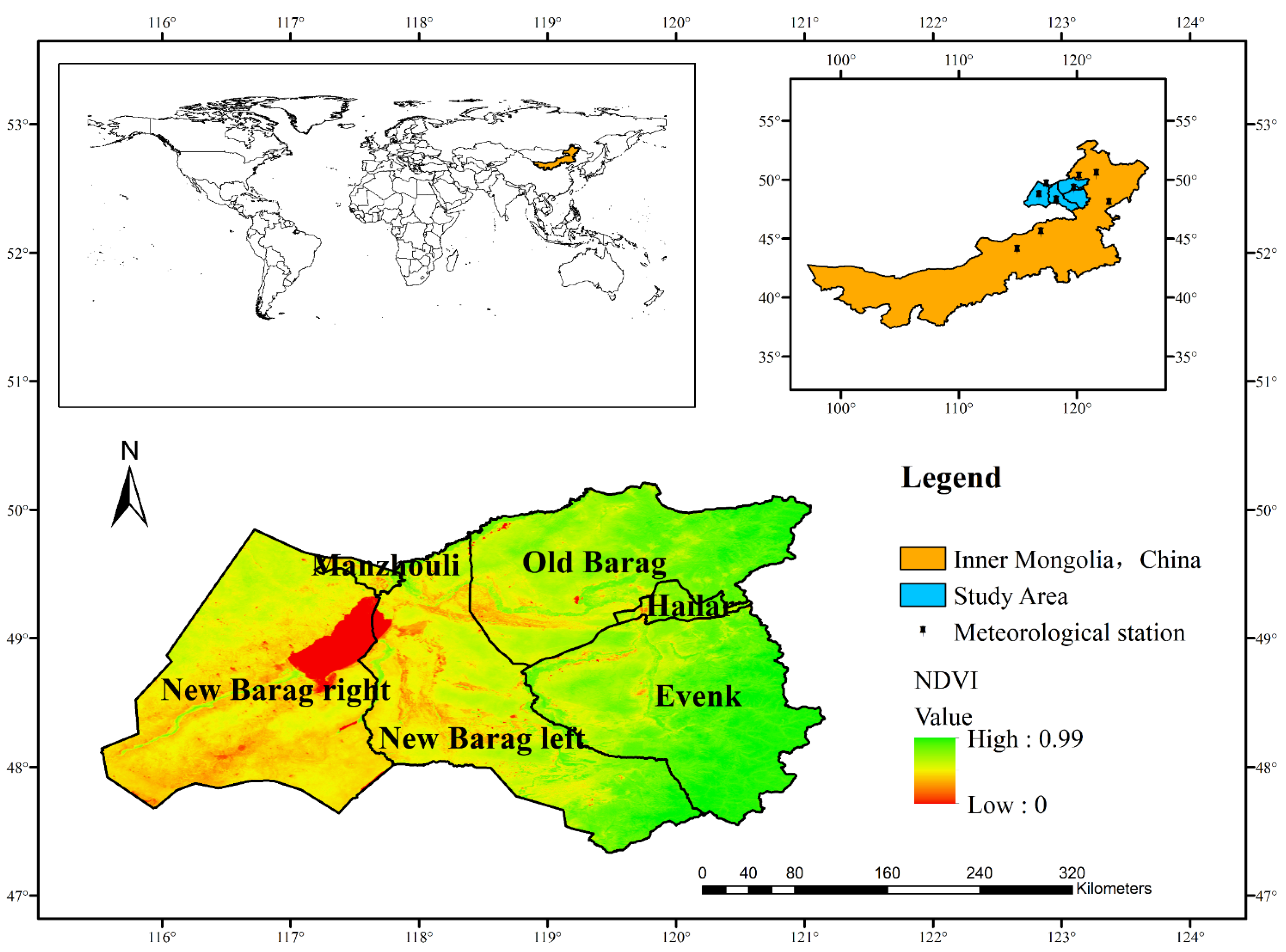
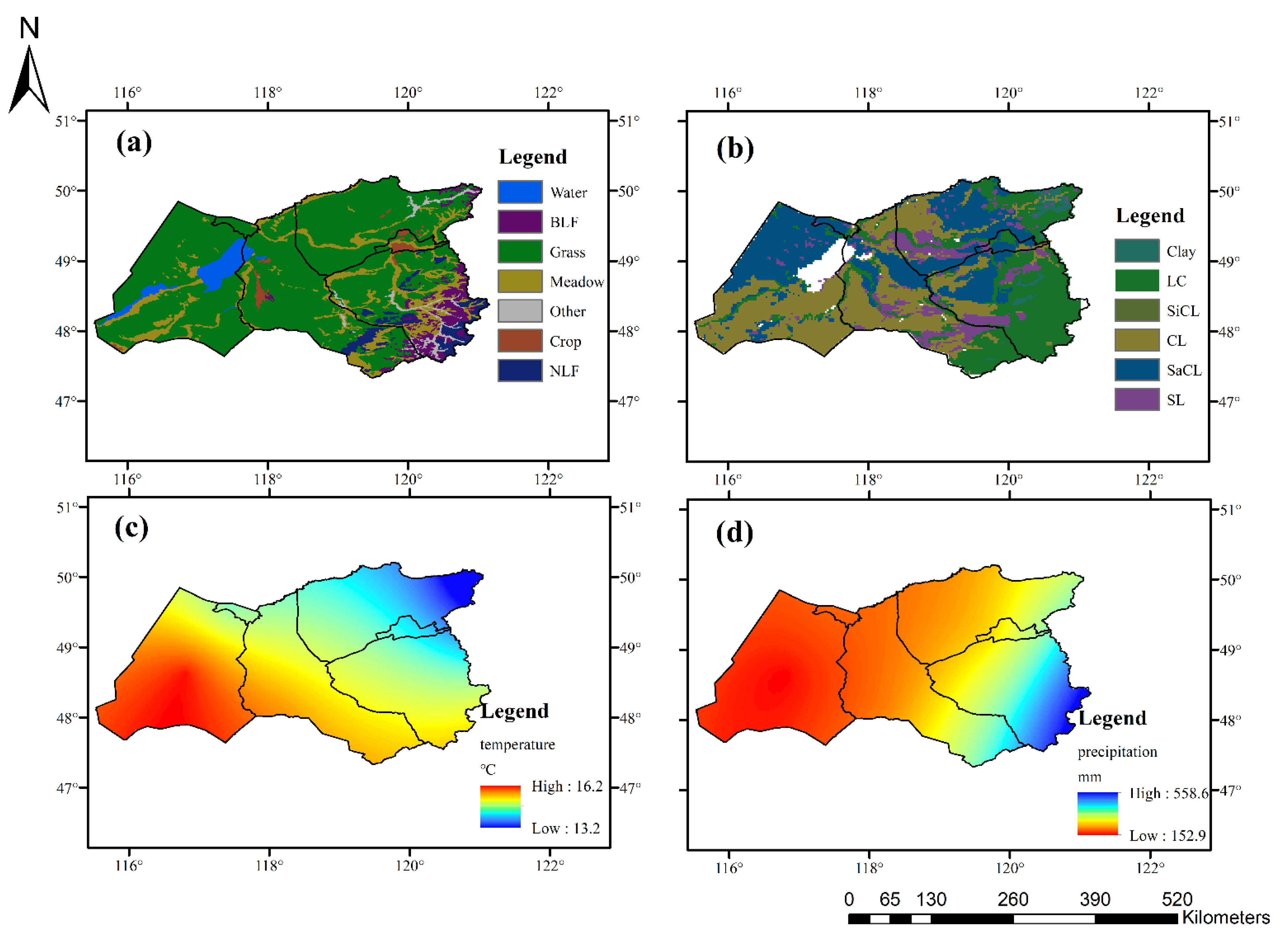
2.1. Study Area

Our study was conducted in southwestern Hulunbuir, Inner Mongolia, China (115°31′–121°12′ E, 47°20′–50°51′ N), which includes two cities (Hailar and Manzhouli) and four banners (Old Barag, New Barag Left, New Barag Right, and Evenk) (Figure 1), and the total area reached 83.6 × 10³ km². The study area exhibits a humid continental climate with long and severe dry winters and short and wet summers [32,33]. The mean annual air temperature is −1 °C. The mean annual precipitation reaches 339 mm, approximately 68% of which is distributed in summer [34,35,36]. In contrast, the annual potential evaporation is approximately 1210 mm [36]. The spatial distribution of the mean temperature is relatively correlated with that of the cumulative precipitation during the growing season (April to August). The western part of the study area exhibits the highest mean temperature and lowest cumulative rainfall during the growing season (Figure 2c,d). Gale winds of a grade higher than eight occur on more than 30 days annually. The elevation in this area ranges from 407 to 1687 m above mean sea level. The main soil types are kastanozems, meadow soil, aeolian soil, chernozems, and gray forest soil [32]. The spatial distribution of soil texture is shown in Figure 2b (including clay, loamy clay, silty clay loam, clay loam, sandy clay loam, sandy loam); the standard for soil texture classification is shown in

Table A1. International system of soil texture classification.

	Abbreviation	Particle Size Composition/%
		Clay	Silt	Sand
sandy soil and sandy loam	SSSL	0–15	0–15	85–100
sandy loam	SL	0–15	0–45	55–85
loam	Loam	0–15	30–45	40–55
silty loam	SiL	0–15	45–100	0–55
sandy clay loam	SaCL	15–25	0–30	55–85
clay loam	CL	15–25	20–45	30–55
silty clay loam	SiCL	15–25	45–85	0–40
sandy clay	SaC	25–45	0–20	55–75
loamy clay	LC	25–45	0–45	10–55
silty clay	SiC	25–45	45–75	0–30
clay	Clay	45–65	0–35	0–55
heavy clay	HC	65–100	0–35	0–35

. Our research area is dominated by perennial grasslands, with a fraction of grassland–forest transition zones, and most of the broadleaf forest and needleleaf forest is located in the east of the study area (Figure 2a). The most common species in this region include Leymus chinensis, Stipa baicalensis, Stipa grandis, Cleistogenes squarrosa, Serratula centauroides, Caragana microphylla, and Pinus sylvestris var. mongolica Litv. [37].

2.2. Data Acquisition

We quantified the NPP from 2000 to 2018 in our study area based on normalized difference vegetation index (NDVI) data extracted from the NASA Moderate-Resolution Imaging Spectroradiometer (MODIS) dataset (MOD13Q1 V006). This remote sensing dataset exhibits a spatial resolution of 250 m and a temporal resolution of 16 days. The variation in vegetation growth during any particular month primarily depends on different climate factors. Thus, we used the maximum value composite (MVC) method to calculate the maximum NDVI value in each month from 2000 to 2018. Vegetation types were identified based on the Chinese vegetation map (1:1,000,000) downloaded from the Chinese Resource and Environment Science and Data Center (http://www.resdc.cn/ (accessed on 4 March 2019)). Soil texture data were collected based on the spatial distribution in the soil texture map of China (1:1,000,000) retrieved from the Chinese National Earth System Science Data Center (http://soil.geodata.cn (accessed on 1 May 2019)). Climate data, including precipitation (PPT), air temperature (Ta), sunshine duration, wind speed, and relative humidity data over 2000–2018, were obtained from meteorological data measured at 9 meteorological stations provided by the National Meteorological Information Center (http://data.cma.cn/ (accessed on 4 March 2019)) (Figure 1). We calculated the daily solar radiation following Food and Agriculture Organization (FAO) guidelines for the computation of crop water requirements, and the formula is shown in Appendix B [38]. The above environmental factors were interpolated via kriging interpolation in ArcMap v.10.5 (ESRI, Redlands, CA, USA, https://www.esri.com/en-us/arcgis/products/index (accessed on 4 March 2019)), which is widely used for the regionalization of various variables at different scales, and subsequent NPP estimation [7,39,40]. We applied the ‘SPEI’ R package to calculate the monthly standardized precipitation evapotranspiration index (SPEI) in order to reflect the drought level [41]. The SPEI calculation process is described in Appendix C. The time spans of all of the data ranged from 2000 to 2018, except that of the vegetation type and soil texture maps. All maps were rescaled to the same spatial resolution (grid size: 0.025°) with the resampling technique in ArcMap v.10.5 (ESRI, Redlands, CA, USA, https://www.esri.com/en-us/arcgis/products/index (accessed on 4 March 2019)).

2.3. Data Analysis

2.3.1. NPP Estimation

NPP is defined as the total amount of photosynthetic gain after the subtraction of vegetation respiratory losses per unit ground area [42]. It is an important component of the terrestrial carbon cycle [7]. Compared to NPP, NDVI is only a qualitative measure of vegetation conditions [43]. Therefore, we calculated $NPP\left(x,t\right)$ based on a light-use efficiency model, namely, the Carnegie Ames Stanford Application (CASA) model [44], with the following equation:

$$NPP\left(x,t\right)=APAR\left(x,t\right)\times \epsilon \left(x,t\right)$$

(1)

where $x$ is the spatial position, $t$ is time, and $APAR\left(x,t\right)$ and $\epsilon \left(x,t\right)$ are the absorbed photosynthetically active radiation (MJ·m⁻²) and light-use efficiency (g·C·mJ⁻¹), respectively.

$APAR\left(x,t\right)$ can be determined with the following equation:

$$APAR\left(x,t\right)=SOL\left(x,t\right)\times FPAR\left(x,t\right)\times 0.5$$

(2)

where $SOL\left(x,t\right)$ is the total solar radiation (calculation method in Appendix B), 0.5 denotes the fraction of the active incoming solar radiation used by vegetation [45], and $FPAR\left(x,t\right)$ is the fraction of photosynthetically active radiation, which can be determined from MODIS NDVI data with the following equations:

$$FPAR\left(x,t\right)=min\left\{\frac{SR\left(x,t\right)-S{R}_{min}}{S{R}_{max}-S{R}_{min}},0.95\right\}$$

(3)

$$SR\left(x,t\right)=\frac{1+NDVI\left(x,t\right)}{1-NDVI\left(x,t\right)}$$

(4)

where $SR\left(x,t\right)$ is the ratio vegetation index, and $S{R}_{max}$ and $S{R}_{min}$ are the 95% and 5% lower quantiles, respectively, of the NDVI [43].

The light-use efficiency $\epsilon \left(x,t\right)$ can be calculated with the following equation [46]:

$$\epsilon \left(x,t\right)=T_{\epsilon 1}\left(x,t\right)\times T_{\epsilon 2}\left(x,t\right)\times W_{\epsilon }\left(x,t\right)\times {\epsilon }^{*}$$

(5)

$$T_{\epsilon 1}\left(x,t\right)=0.8+0.02T_{opt}-0.0005{(T_{opt})}^2$$

(6)

$$\begin{array}{cc}\hfill T_{\epsilon 2}=1.1814/& {\displaystyle \{}\left\{1+\exp (0.2\times \left(T_{opt}-10-Ta\left(t\right)\right))\right\}\hfill \\ & \times \left\{1+\exp (0.3\times \left(-T_{opt}-10+Ta\left(t\right)\right))\right\}{\displaystyle \}}\end{array}$$

(7)

$$W_{\epsilon }=0.5+0.5\times \frac{AET}{PET}$$

(8)

where $T_{\epsilon 1}\left(x,t\right)$ denotes the limitation of extremely low and high temperatures imposed on the light-use efficiency, and $T_{\epsilon 2}\left(x,t\right)$ denotes the light-use efficiency when the temperature reaches above or below $T_{opt}$ [47]. $T_{opt}$ is the average air temperature in months when the maximum NDVI value is reached throughout the year, and $Ta\left(t\right)$ is the average air temperature in month t. $W_{\epsilon }$ is a coefficient of the water stress, and $AET$ denotes the actual evapotranspiration (mm), which can be calculated with the method of Zhou and Zhang [48]. $PET$ is the potential evapotranspiration, which can be calculated with the FAO Penman–Monteith (P–M) method [38]. In addition, ε^* is the maximum light-use efficiency value and depends on the vegetation type [49].

$$AET=\frac{PPT\times R_n\left(PP{T}^2+R_n{}^2+PPT\times R_n\right)}{\left(PPT+R_n\right)\times \left(PP{T}^2+R_n{}^2\right)}$$

(9)

$$PET=\frac{0.408\Delta \left(R_n-G\right)+\gamma \frac{900}{Ta+273}{U}_2\left(e_s-e_a\right)}{\Delta +\gamma \left(1+0.34U_2\right)}$$

(10)

where $PPT$ denotes precipitation (mm); $R_n$ is the net radiation (MJm⁻²·day⁻¹), which is calculated by Formula (A10) in Appendix B; $\Delta$ is the slope of the vapor pressure curve (kPa·°C⁻¹); $G$ is the soil heat flux density (MJ·m⁻²·day⁻¹), which is small and can be neglected; $\gamma$ is a psychrometric constant (kPa·°C⁻¹); $Ta$ is the mean daily temperature (°C); $U_2$ is the wind speed at 2 m above ground level (m·s⁻¹); $e_s$ is the mean saturation vapor pressure (kPa); and $e_a$ is the actual vapor pressure (kPa). The calculations of $\Delta$, $\gamma$, $U_2$, $e_s$, and $e_a$ are shown in Appendix D.

2.3.2. Time Lag Estimation

• Partial correlation coefficient (PCC) method

The PCC was used to determine the relationship between $NPP$ and three climate conditions (i.e., $PPT$, $Ta$, and $SPEI$). For example, the PCC for $PPT$ is calculated according to:

$$R_{NPP,PPT}=\frac{{{\displaystyle \sum }}_{i=1}^n\left[\left(PP{T}_i-\overline{PPT}\right)\times \left(NP{P}_i-\overline{NPP}\right)\right]}{\sqrt{{{\displaystyle \sum }}_{i=1}^n{\left(PP{T}_i-\overline{PPT}\right)}^2-{{\displaystyle \sum }}_{i=1}^n{\left(NP{P}_i-\overline{NPP}\right)}^2}}$$

(11)

$$R_{NPP PPT,Ta}=\frac{R_{NPP PPT}-R_{NPP Ta}\times R_{PPT Ta}}{\sqrt{1-R_{NPP Ta}{}^2}\sqrt{1-R_{PPT Ta}{}^2}}$$

(12)

$$PC{C}_{NPP PPT,Ta SPEI}=\frac{R_{NPP PPT,Ta}-R_{NPP SPEI, Ta}\times R_{PPT SPEI, Ta}}{\sqrt{1-R_{NPP SPEI, Ta}{}^2}\sqrt{1-R_{PPT SPEI, Ta}{}^2}}$$

(13)

where $R_{NPP,PPT}$ is the correlation coefficient between the $NPP$ and $PPT$ variables; $PP{T}_i$ and $NP{P}_i$ denote the values of the $PPT$ and $NPP$ variables, respectively, in year$i$; and n represents the year range (n = 19, in this study). $\overline{PPT}$ and $\overline{NPP}$ represent the average $PP{T}_i$ and $NP{P}_i$ values, respectively. $R_{NPP PPT,Ta}$ is the PCC between $NPP$ and $PPT$ controlled for the $Ta$ value. $PC{C}_{NPP PPT,Ta SPEI}$ is the PCC between $NPP$ and $PPT$ when we controlled $Ta$ and $SPEI$. The significance of the results was examined via the t-test.

Previous studies suggested that the effect of climate conditions could persist into the next season, and the time lag was assumed to be limited to shorter than 6 months [50,51]. Thus, in this study, we considered a time lag ranging from 0 to 5 months. We calculated the PCC between $NPP$ and $PPT$,$Ta$, and $SPEI$ in each lagged month ($PC{C}_i$, for $i$ = 0, 1, …, 5). The maximum absolute PCC value was selected as the final correlation coefficient ($PC{C}_{best}$) between $NPP$ and each climate condition:

$$PC{C}_{best}=PC{C}_i, when PC{C}_i=maximum\left\{R_{0-5}\right\}$$

(14)

$$BTL=i, when PC{C}_i=maximum\left\{R_{0-5}\right\}$$

(15)

where$BTL$ denotes the best time lag of $NPP$ response to the specific climate conditions.

2.

Multiple linear regression model method

This method first assumes that the analyzed climatic conditions limit NPP accumulation and that the impact of climatic conditions at different times on vegetation productivity exhibits a certain continuity and accumulation effect over time [52]. In this study, we considered a time lag ranging from 0 to 5 months. First, $NPP$, $PPT$, $Ta$, and $SPEI$ were standardized at the monthly scale over the growing season. Since the data were standardized before fitting, the coefficient of the independent variables in the fitting regression Equations (16)–(18) reflects the magnitude of the influence of climate conditions on NPP.

$$NP{P}_{t,PPT}=\sum a_{m}PP{T}_m+D\left(m=t, t-1, t-2, \dots ,t-5\right)$$

(16)

$$NP{P}_{t,Ta}=\sum b_{m}T{a}_m+E\left(m=t, t-1, t-2, \dots ,t-5\right)$$

(17)

$$NP{P}_{t,SPEI}=\sum c_{m}SPE{I}_m+F\left(m=t, t-1, t-2, \dots ,t-5\right)$$

(18)

where $NP{P}_{t,PPT}$, $NP{P}_{t,Ta}$, and $NP{P}_{t,SPEI}$ are $NPP$ in month $\mathrm{t}$ determined via $PPT$, $Ta$, and $SPEI$fitting, respectively. $PP{T}_m$, $T{a}_m$, and $SPE{I}_m$ denote the monthly $PPT$, $Ta$, and $SPEI$, respectively, in month $m$. Furthermore, $a_m$, $b_m$, and $c_m$ denote the coefficients of $PPT$, $Ta$, and $SPEI$, respectively, in month $m$. $D$, $E$, and $F$ denote the intercepts of the $PPT$, $Ta$, and $SPEI$ fitting equations, respectively.

$$BT{L}_{PPT}=m, when a_m=maximum\left(a_m,m=t, t-1, t-2, \dots ,t-5\right)$$

(19)

$$BT{L}_{Ta}=m, when b_m=maximum\left(b_m,m=t, t-1, t-2, \dots ,t-5\right)$$

(20)

$$BT{L}_{SPEI}=m, when c_m=maximum\left(c_m,m=t, t-1, t-2, \dots ,t-5\right)$$

(21)

where $BT{L}_{PPT}$, $BT{L}_{Ta}$, and $BT{L}_{SPEI}$ denote the BTL values of the $NPP$ response to $PPT$, $Ta$, and $SPEI$, respectively.

The same result from the PPC method and the regression method was then extracted for further statistical analysis in Section 3.2.

2.3.3. The Geodetector Model

The Geodetector model is a new spatial statistical tool for exploring spatial heterogeneity and quantitatively evaluating the contribution of driving factors [53]. This tool comprises four modules, namely, factor detector, ecological detector, risk detector, and interaction detector. To examine the impact of various vegetation types (including broadleaf forest, needleleaf forest, grass, meadow, and crop) and soil textures (including sandy loam, sandy clay loam, clay loam, silty clay loam, loamy clay, and clay) on the spatial pattern of the best time lag of the NPP response to PPT, Ta, and SPEI, we used the factor detector and interaction detector.

Using the factor detector model to detect vegetation type or soil texture can explain the spatial differentiation of the best time lag through the q value. The larger the q value is, the higher the explanatory power of vegetation type and soil texture for the best time lag. The interaction detector can identify the interaction effect on the best time lag between vegetation type and soil texture. The definition of the various interaction types in the interaction detector is provided in

Table 1. Definition of the interaction types in the interaction detector.

Interaction Relationship	Interaction Types
q(X1∩X2) < Min [q(X1), q(X2)]	Nonlinear weakened
Min [q(X1), q(X2)] < q(X1∩X2) < Max [q(X1), q(X2)]	Univariable weakened
q(X1∩X2) = q(X1) + q(X2)	Independent
Max(q(X1), q(X2)) < q(X1∩X2) < q(X1) + q(X2)	Bivariable enhanced
q(X1∩X2) > q(X1) + q(X2)	Nonlinear enhanced

.

PCC analysis was performed in ArcMap v.10.5 software based on pixels (0.025°). The ‘GD’ R package was used to calculate the q value for the factor detector and interaction detector [54].

3. Results

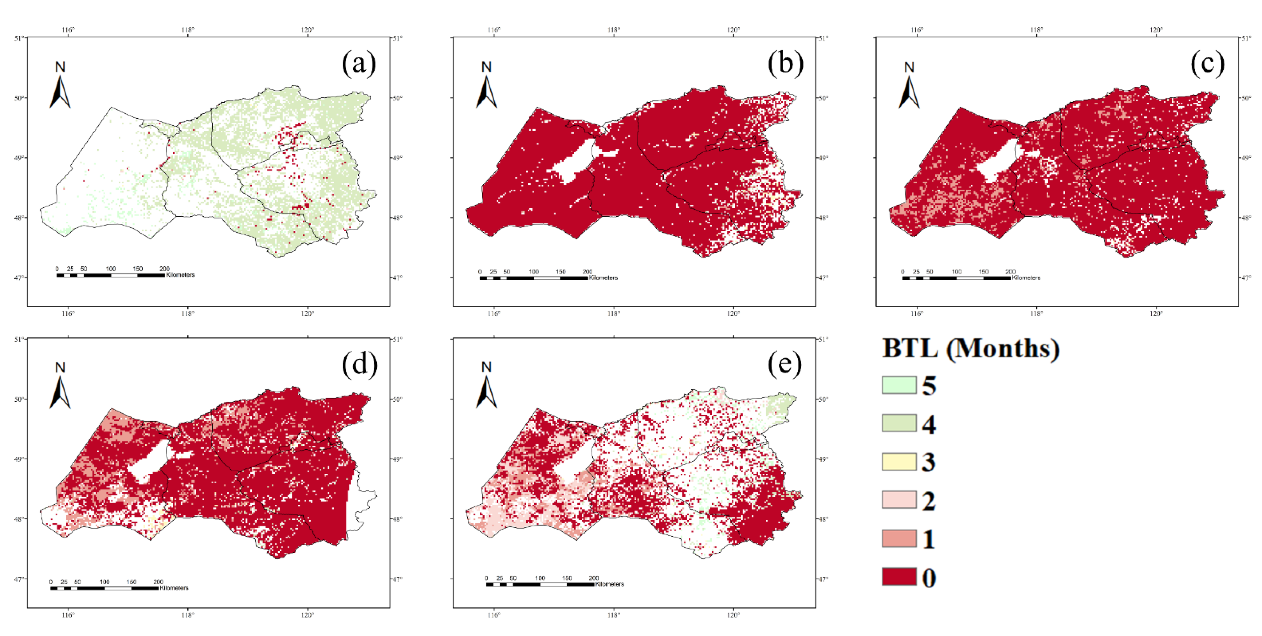
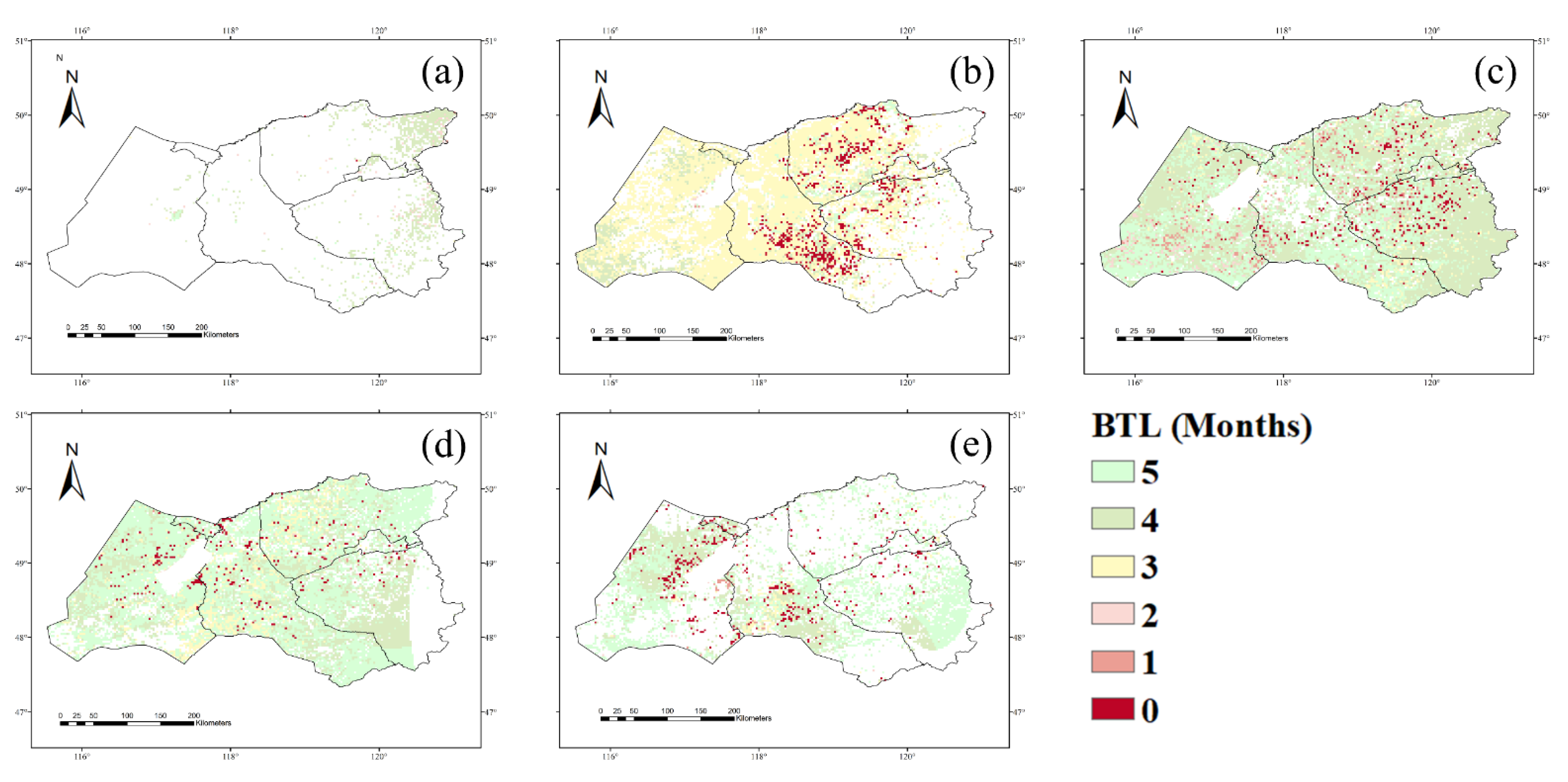
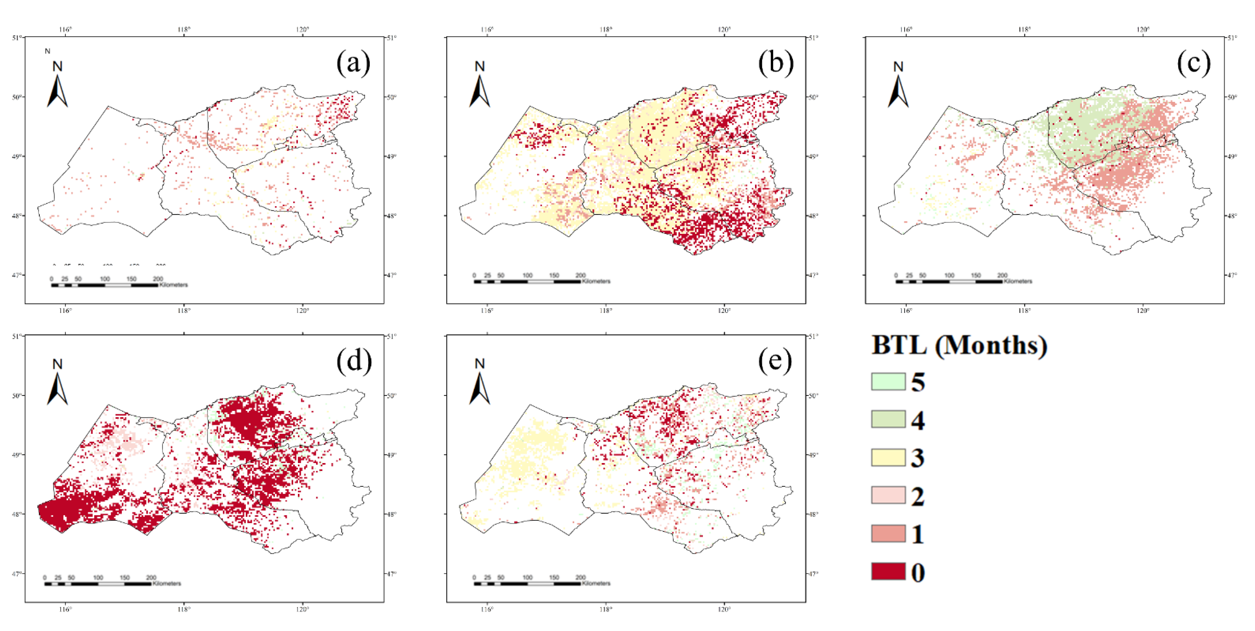
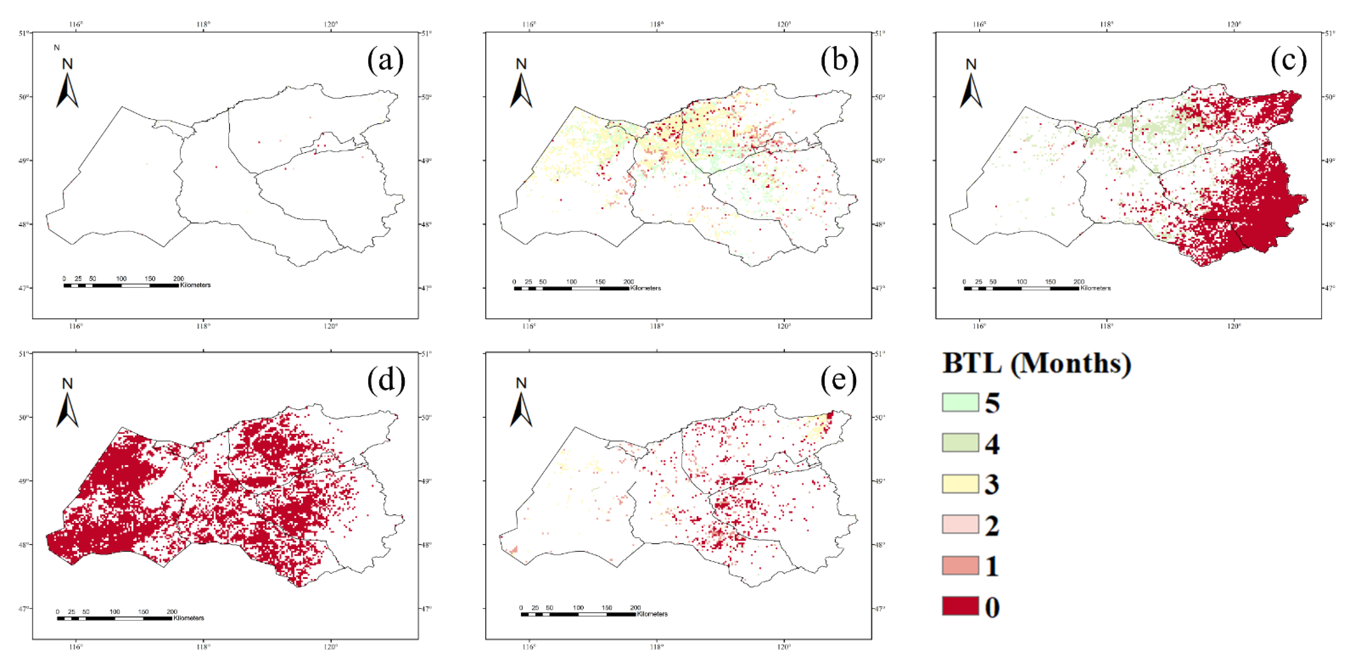
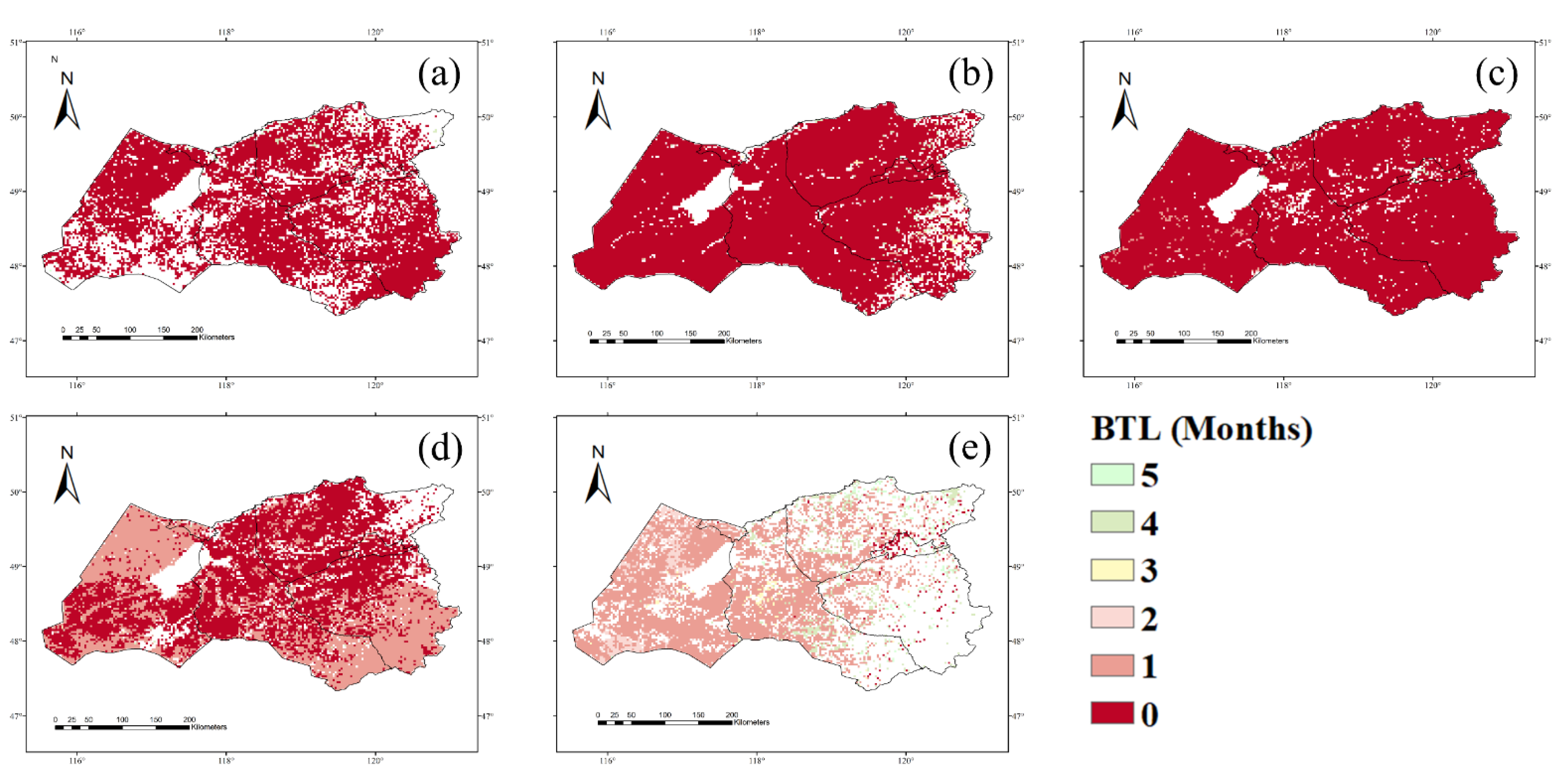
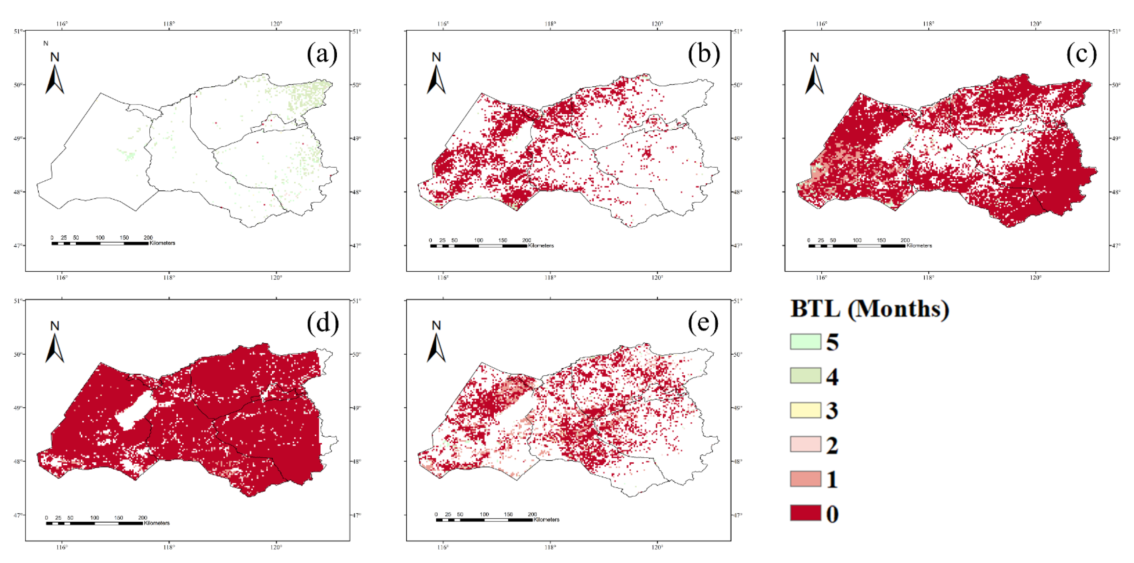
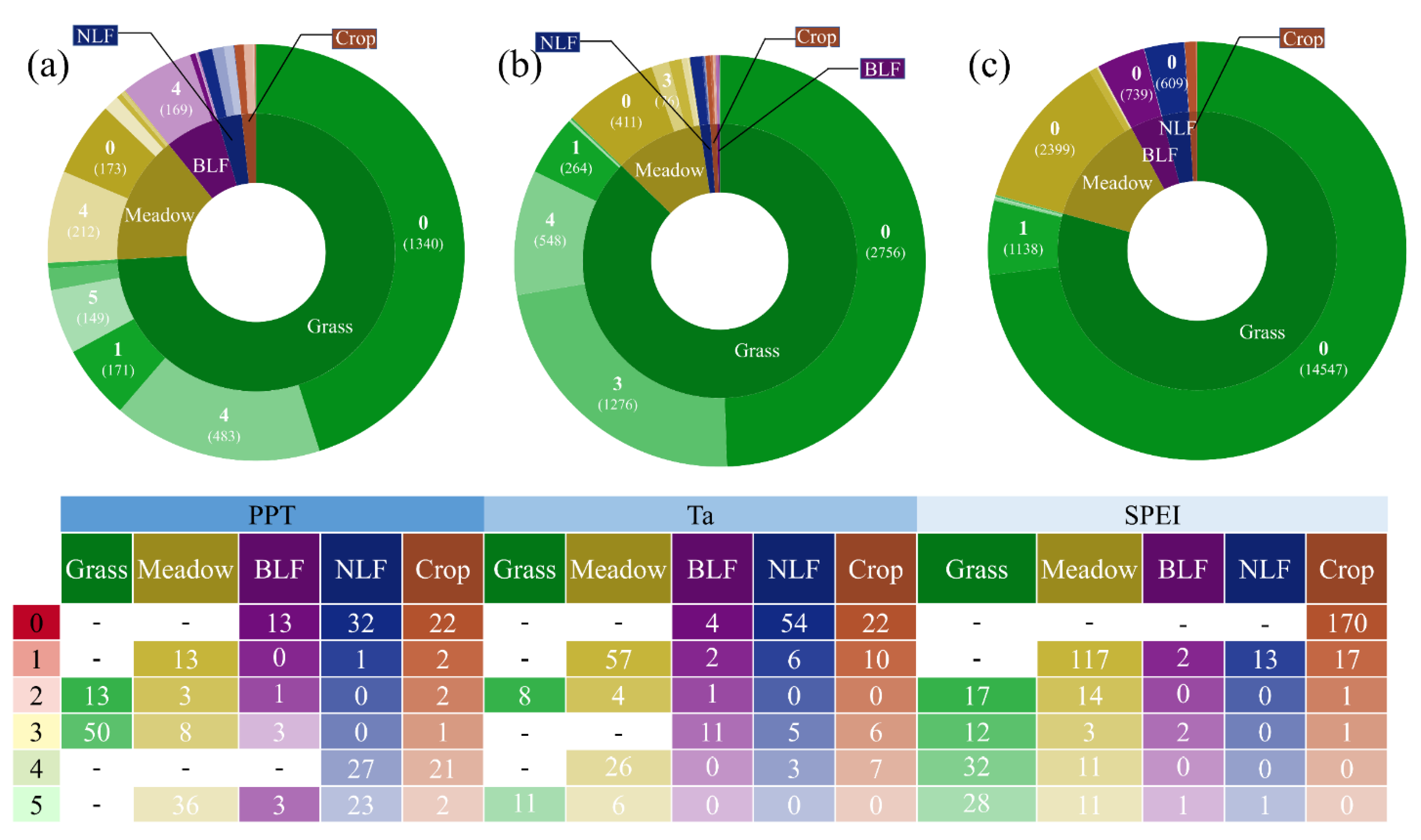
3.1. NPP Response to Climate Conditions with Varied Time Lags

Spatial distributions of the best time lag of the NPP response to PPT, Ta, and SPEI are shown in Figure 3, Figure 4, Figure 5, Figure 6, Figure 7 and Figure 8. We found that the time-lagged response significantly varied among the different months and climate conditions. Regarding PPT, Figure 3 and Figure 4 show the best time lag estimated with the above two methods. Both methods also revealed that NPP in April was significantly affected by PPT in the preceding 4 months (precipitation in December of the previous year). With regard to time-lag effects of the NPP response to Ta (Figure 5 and Figure 6), NPP in April was slightly affected by Ta. In July, NPP indicated no apparent lagged effects. The effects of Ta on NPP in the remaining analysis months were significantly delayed, but there occurred no obvious regularity.

Regarding time-lag effects in NPP with respect to the SPEI, the SPEI imposed a significant instantaneous effect (0 month) on NPP from May to July (Figure 7b–d and Figure 8b–d). With the use of the PCC method, in August, NPP in most areas (i.e., 78.16% of all grids) was influenced by the SPEI in the preceding month (Figure 7e). Based on the regression method, in August, NPP in some grids within the study area also indicated that the best time lag reached 1 month (Figure 8e).

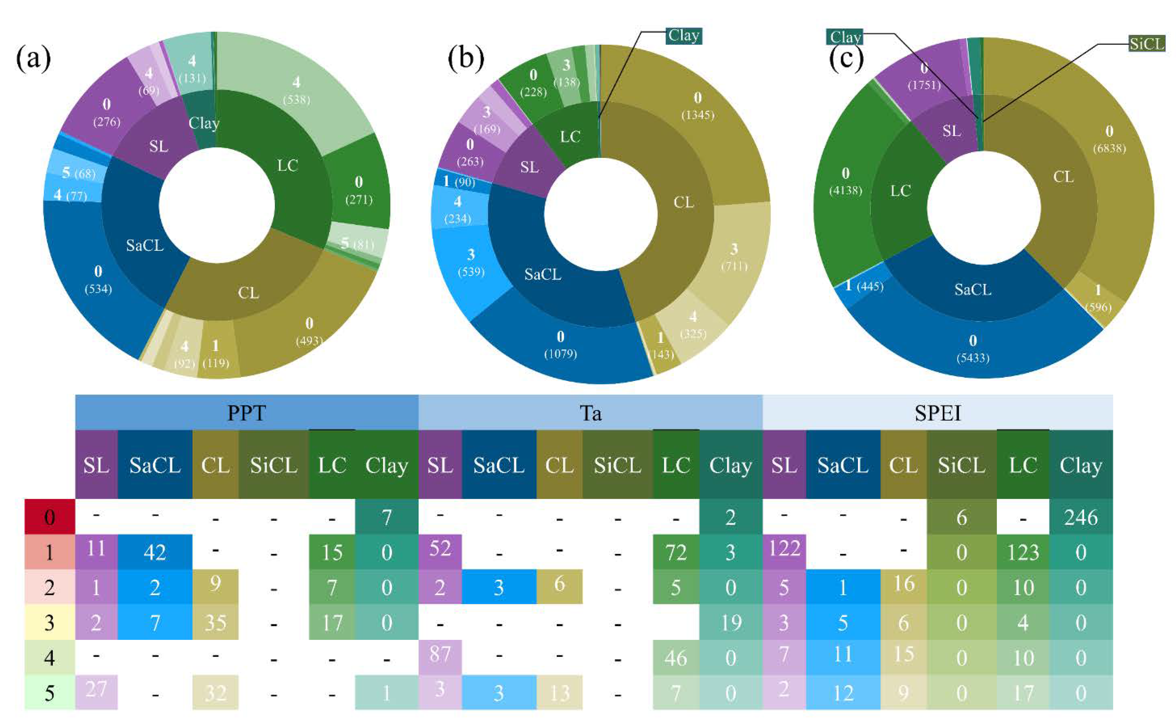
3.2. Time-Lag Effects of Climate Conditions on NPP with Vegetation Type and Soil Texture

The best time lags of the NPP response to PPT, Ta, and SPEI among the various vegetation types are shown in Figure 9. Regarding PPT, the 0- and 4-month lags attained the highest frequency among all vegetation types (Figure 9a). The largest proportion of the best time lag in grass (60.74%) and crop (44.00%) was 0 months, and the largest proportion of best time lag in meadow (47.64%) and broadleaf forest (89.42%) was 4 months. In needleleaf forest, 0- and 4-month lags accounted for 38.55% and 32.53%, respectively. With regard to Ta, the area of 0-month lag was larger among all vegetation types except the broadleaf forest type (Figure 9b). Grass and meadow were also influenced by Ta in the preceding 3 months. Furthermore, 0-month lag was the most frequently observed in the NPP response to SPEI among all vegetation types (Figure 9c). Certain areas of grass and meadow also indicated a 1-month lag.

The variation in the best time lag of the NPP response to PPT, Ta, and SPEI across different soil textures is shown in Figure 10. Regarding PPT, most sandy loam, sandy clay loam, and clay loam areas exhibited a 0-month lag, while loamy clay and clay areas exhibited 4-month lag (Figure 10a). In terms of Ta among all best time lag values, the 0-month lag accounted for more than 45.74% across all soil textures (Figure 10b). The 0~1-month best time lag of NPP response to SPEI occupied a larger area among all soil textures (Figure 10c).

The spatial variation in the legacy effects of PPT, Ta, and SPEI may contribute to the different vegetation types and soil textures. The factor detector module was employed to evaluate the effect of vegetation type and soil texture on the best time lag, and the results are listed in

Table 2. Q values for factor detector and interaction detector modules.

	Vegetation Types	Soil Textures	Vegetation Types ∩ Soil Textures
PPT	0.15 **	0.31 **	0.37
Ta	0.10 **	0.04 **	0.13
SPEI	0.00	0.00	0.00

Note: ** denotes 0.01 significance level.

. Regarding the best time lag of the NPP response to PPT, the q values for the vegetation type and soil texture factors were 0.15 and 0.31, respectively. The results indicated that the various vegetation types and soil textures could explain 15% and 31%, respectively, of the change in the best time lag of the NPP response to PPT. With regard to the best time lag of the NPP response to Ta and SPEI, the q values for the vegetation type and soil texture factors were all less than 0.1, which suggested that vegetation type and soil texture slightly influenced the spatial variation in the best time lag. The interactive effects between the vegetation type and soil texture factors on the best time lag were identified with the interaction detector module. The q values for the interaction effect between the vegetation type and soil texture factors on the best time lag of the NPP response to PPT and Ta were all greater than those for a single factor (Table 2), which indicated that the interaction effect between the vegetation type and soil texture factors was bivariable enhanced.

4. Discussion

4.1. Time Lags of the NPP Response to Precipitation, Temperature, and Drought

In line with the findings of other researchers [16,55,56], there occurred a notable legacy effect of climate conditions, where vegetation growth was significantly affected by PPT, Ta, and SPEI in preceding months. Previous studies of ecotones determined that the ecotone migration response to climate warming was gradual, exhibiting a lag effect due to the resistance of retreating forest biomes [28]. This result is similar to ours in the considered forest–grassland ecotone, and details and a comparison are provided in

Table 3. Comparison of present findings to those of other studies.

Climate Conditions	Time Lag	Timescale	Study Area	Time Span	Reference
precipitation	4-month lag	monthly scale	Hulunbuir	2000–2018	in this study
	0.55 ± 0.95-month lag	monthly scale	Global	1982–2015	[57]
	7.9~17.7-day lag	daily	The Chinese Loess Plateau	1982–2015	[58]
	40-day lag	daily	Grasslands National Park, southern Saskatchewan, Canada	1985–2007	[59]
temperature	0~4-month lag	monthly scale	Hulunbuir	2000–2018	in this study
	0.56 ± 1.04-month lag	monthly scale	Global	1982–2015	[57]
	3-month lag	seasonal scale	China	1982–1999	[55]
	6.2~25.3-day lag	daily	The Chinese Loess Plateau	1982–2015	[58]
	10-day lag	daily	Grasslands National Park, southern Saskatchewan, Canada	1985–2007	[59]
drought	0~2-month lag	monthly scale	Hulunbuir	2000–2018	in this study
	2~3-month lag	seasonal scale	The Chinese Loess Plateau	2000–2010	[56]
	2-month lag	seasonal scale	Southern Africa	2015–2016	[16]
	8-month lag	seasonal scale	Southern Africa	2015–2016	[16]
solar radiation	0.50 ± 0.94-month lag	monthly scale	Global	1982–2015	[57]
soil water availability	2–9-month lag		Kessler Farm Field Laboratory, Central Redbed Plains of Oklahoma	From 20 February 2003 to 20 February 2004	[60]

[16,55,57,58,59,60]. In previous studies of the time-lag effect, the time lag ranged from 6.2 days to 9 months at the daily, monthly, and annual scales. Compared to other studies, there existed a longer time-lag effect in the NPP response to precipitation in this study. We found that NPP in April was influenced by PPT in the preceding 4 months, and a similar result was obtained in previous studies [1]. There are two reasons that could explain this result. First, a PPT deficit commonly occurs in spring, but vegetation growth may not be affected [32,33]. PPT in winter constitutes a major water source in April for vegetation growth in our study region [61]. Second, PPT in winter in the form of snow further generates suitable snowpack, which can increase the temperature of soil surface layers and protect vegetation from injury due to chilling and freezing [62]. Additionally, in other ecotones, researchers also found that the time lag in vegetation response to rainfall was 1–2 months [63].

Our results revealed that the SPEI imposed a significant instantaneous effect on most NPP values from May to July, and a 1-month legacy was found in July and August. Other researchers also determined that a late growing season drought could cause more notable drought legacy effects [64]. This phenomenon can be attributed to vegetation exhibiting a particular vulnerability to drought at the early stages of growth. Vegetation can obtain a well-developed functional structure and drought-resistance strategies, and vegetation can adjust water-use efficiency under dry conditions at later stages of growth [65]. The present SPEI slightly affected NPP, but a legacy effect still occurred. Similar findings were obtained in previous studies [56]. In our research, we did not determine an obvious trend in the spatiotemporal heterogeneity of Ta legacy effects. This result may be explained by the fact that Ta, compared to PPT and SPEI, is not the dominant climate factor during the growing season in our study area [66]. Moreover, a similar result was found in other research in which correlations between temperature and NPP mostly depended on precipitation in the semiarid grassland ecosystem of northern China [40]. Therefore, the effect of Ta was probably offset by the effects of PPT and SPEI.

4.2. Time-Lag Effects of the NPP Response to Precipitation, Temperature, and Drought with Different Vegetation Types and Soil Textures

Diverse vegetation types and soil textures occur in the Hulunbuir grassland, which is a forest–grassland ecotone. Our results indicated that the time lag lengths of PPT, Ta, and SPEI on NPP varied in the different grids (Figure 3, Figure 4, Figure 5, Figure 6, Figure 7 and Figure 8). This phenomenon could be explained by the different vegetation types and soil textures.

Compared to grass and crop, broadleaf forest and meadow exhibited longer time-lag effects of PPT during the growing season. There are certain potential reasons for this phenomenon. First, this finding may be explained by the different hydrothermal conditions. In this study, broadleaf forest was located in a region with high PPT and low Ta levels (Figure 2a), which could lead to reduced evapotranspiration. Thus, preceding PPT was stored for subsequent vegetation growth. Similarly, meadows also exhibit better hydrothermal conditions than those of grass and crop. Second, the remaining PPT can enter the deeper soil through infiltration and can be stored in soil. Compared to grass and crop, broadleaf forests with strong root systems can take up water from relatively deep sites [10,67]. Third, broadleaf forests and meadows achieve a higher capacity to regulate the microclimate, and the preceding PPT can be reallocated. Researchers found that both near-ground solar radiation and soil temperature decreased with increasing canopy cover, and these interactive effects are relevant for key ecohydrological processes, such as soil evaporation [68].

The lag effect length of Ta was shorter in needleleaf forest than in other vegetation types during the growing season. This finding does not agree with the results of Sui et al. [69]. They found that grass generated a more sensitive response to Ta than did forest across temperate grasslands in China at the annual scale. In our research, forests were mostly located in regions containing abundant water resources and low temperatures [31]. These conditions resulted in greater restriction of forest by Ta and a higher sensitivity to Ta variation during the early growing season than that of grass. A similar result was also reported in a previous study [70].

Our study found that broadleaf forests and needleleaf forests exhibited shorter time-lag effects of the SPEI than did grass and meadow during the growing season. Researchers also found that forest had a high demand for water and heat. Forests efficiently use water originating from PPT and heat obtained from air at a high temperature within a short time, resulting in shorter time-lag effects [57].

In addition to vegetation type, our results indicated that the lags in the NPP response to PPT increased with increasing soil clay content during the growing season. This result may be related to the different water-holding capacities of soils with different textures. Compared to sandy soil, clay soil can preserve a considerably higher level of soil moisture [21]. Therefore, the stress effect of water on vegetation NPP in clay soil is less than that in sand soil.

Best time lag changes are not influenced by a single factor but by the overall interaction effect between the vegetation type and soil texture factors. Previous studies indicated that the interaction effect of two factors was always greater than that of a single factor [53]. In this study, the interaction effect between the vegetation type and soil texture factors indicated enhancement. Although the maximum interpretation of single factors reached only 31%, these factors could be enhanced upon interaction with other factors.

5. Conclusions

Analysis of the time-lag effect of precipitation, temperature, and drought on NPP at the seasonal scale suggests the following patterns. First, there occurred time-lag effects of precipitation and drought on NPP. This result further revealed that moisture was the major factor limiting vegetation in the considered temperate forest–grassland ecotone. Second, a legacy effect of drought on NPP occurred at the later stages of vegetation growth, resulting from the well-developed functional structure and drought-resistance strategies of vegetation in semiarid areas. Due to water retention and water use strategies, a legacy effect of precipitation also occurred at the early stages of vegetation growth. Third, the time-lag effect of precipitation on NPP varied with vegetation type and soil texture between the different spatial patterns during the growing season. The spatial pattern of the time lag was influenced by the interaction effect between the vegetation type and soil texture factors. Our time-lag effects findings help to clarify the vegetation–climate relationship in temperate semiarid forest–grassland ecotones. However, the time-lag effect of climate conditions on vegetation growth in forest–grassland ecotones is inadequately considered at the global scale. Thus, it remains challenging but crucial to capture these processes in dynamic vegetation models in order to obtain a better understanding of vegetation responses to climate change.

References

1. Jia, X.; Zha, T.; Gong, J.; Wang, B.; Zhang, Y.; Wu, B.; Qin, S.; Peltola, H. Carbon and water exchange over a temperate semi-arid shrubland during three years of contrasting precipitation and soil moisture patterns. Agric. For. Meteorol. 2016, 228–229, 120–129. [Google Scholar] [CrossRef]
2. Reichstein, M.; Bahn, M.; Ciais, P.; Frank, D.; Mahecha, M.D.; Seneviratne, S.I.; Zscheischler, J.; Beer, C.; Buchmann, N.; Frank, D.C.; et al. Climate extremes and the carbon cycle. Nature 2013, 500, 287–295. [Google Scholar] [CrossRef] [PubMed]
3. Seneviratne, S.I.; Zhang, X.; Adnan, M.; Badi, W.; Dereczynski, C.; Di Luca, A.; Ghosh, S.; Iskandar, I.; Kossin, J.; Lewis, S.; et al. Weather and Climate Extreme Events in a Changing Climate. In Climate Change 2021: The Physical Science Basis; Contribution of Working Group I to the Sixth Assessment Report of the Intergovernmental Panel on Climate Change; Masson-Delmotte, V., Zhai, P., Pirani, A., Connors, S.L., Péan, C., Berger, S., Caud, N., Chen, Y., Goldfarb, L., Gomis, M.I., et al., Eds.; Cambridge University Press: Cambridge, UK, 2021; in press. [Google Scholar]
4. Compagnoni, A.; Levin, S.; Childs, D.Z.; Harpole, S.; Paniw, M.; Römer, G.; Burns, J.H.; Che-Castaldo, J.; Rüger, N.; Kunstler, G.; et al. Herbaceous perennial plants with short generation time have stronger responses to climate anomalies than those with longer generation time. Nat. Commun. 2021, 12, 1824. [Google Scholar] [CrossRef] [PubMed]
5. Yuan, Z.; Wang, Y.; Xu, J.; Yin, J.; Chen, S. Effects of Hydrothermal Conditions on the Net Primary Productivity in the Source Region of Yangtze River, China. Sci. Rep. 2021, 11, 1376. [Google Scholar] [CrossRef]
6. Wang, Z.; Zhang, Y.; Yang, Y.; Zhou, W.; Gang, C.; Zhang, Y.; Li, J.; An, R.; Wang, K.; Odeh, I.; et al. Quantitative assess the driving forces on the grassland degradation in the Qinghai–Tibet Plateau, in China. Ecol. Inform. 2016, 33, 32–44. [Google Scholar] [CrossRef]
7. Liu, C.; Dong, X.; Liu, Y. Changes of NPP and their relationship to climate factors based on the transformation of different scales in Gansu, China. Catena 2015, 125, 190–199. [Google Scholar] [CrossRef]
8. Zhang, L.; Guo, H.; Ji, L.; Lei, L.; Wang, C.; Yan, D.; Li, B.; Li, J. Vegetation greenness trend (2000 to 2009) and the climate controls in the Qinghai-Tibetan Plateau. J. Appl. Remote Sens. 2013, 7, 073572. [Google Scholar] [CrossRef]
9. Li, B.; Huang, F.; Qin, L.; Qi, H.; Sun, N. Spatio-Temporal Variations of Carbon Use Efficiency in Natural Terrestrial Ecosystems and the Relationship with Climatic Factors in the Songnen Plain, China. Remote Sens. 2019, 11, 2513. [Google Scholar] [CrossRef] [Green Version]
10. Sala, O.E.; Gherardi, L.A.; Reichmann, L.; Jobbágy, E.; Peters, D. Legacies of precipitation fluctuations on primary production: Theory and data synthesis. Philos. Trans. R. Soc. B Biol. Sci. 2012, 367, 3135–3144. [Google Scholar] [CrossRef] [Green Version]
11. Arnone, J.A., III; Verburg, P.S.J.; Johnson, D.W.; Larsen, J.D.; Jasoni, R.L.; Lucchesi, A.J.; Batts, C.M.; Von Nagy, C.; Coulombe, W.G.; Schorran, D.E.; et al. Prolonged suppression of ecosystem carbon dioxide uptake after an anomalously warm year. Nature 2008, 455, 383–386. [Google Scholar] [CrossRef]
12. Wu, D.H.; Zhao, X.; Liang, S.L.; Zhou, T.; Huang, K.C.; Tang, B.J.; Zhao, W.Q. Time-lag effects of global vegetation responses to climate change. Glob. Change Biol. 2015, 21, 3520–3531. [Google Scholar] [CrossRef]
13. Li, X.; Liu, M.; Hajek, O.L.; Yin, G. Different Temporal Stability and Responses to Droughts between Needleleaf Forests and Broadleaf Forests in North China during 2001–2018. Forests 2021, 12, 1331. [Google Scholar] [CrossRef]
14. Zhang, Y.; Wang, X.; Li, C.; Cai, Y.; Yang, Z.; Yi, Y. NDVI dynamics under changing meteorological factors in a shallow lake in future metropolitan, semiarid area in North China. Sci. Rep. 2018, 8, 15971. [Google Scholar] [CrossRef] [Green Version]
15. Zhang, Q.; Kong, D.; Shi, P.; Singh, V.P.; Sun, P. Vegetation phenology on the Qinghai-Tibetan Plateau and its response to climate change (1982–2013). Agric. For. Meteorol. 2018, 248, 408–417. [Google Scholar] [CrossRef]
16. Marumbwa, F.M.; Cho, M.A.; Chirwa, P.W. An assessment of remote sensing-based drought index over different land cover types in southern Africa. Int. J. Remote Sens. 2020, 41, 7368–7382. [Google Scholar] [CrossRef]
17. Zhao, W.; Zhao, X.; Zhou, T.; Wu, D.; Tang, B.; Wei, H. Climatic factors driving vegetation declines in the 2005 and 2010 Amazon droughts. PLoS ONE 2017, 12, e0175379. [Google Scholar] [CrossRef]
18. Huang, N.; Wang, L.; Song, X.-P.; Black, T.A.; Jassal, R.S.; Myneni, R.B.; Wu, C.; Song, W.; Ji, D.; Yu, S.; et al. Spatial and temporal variations in global soil respiration and their relationships with climate and land cover. Sci. Adv. 2020, 6, eabb8508. [Google Scholar] [CrossRef]
19. Hu, Y.; Yao, Y.; Kou, Z. Exploring on the climate regionalization of Qinling-Daba mountains based on Geodetector-SVM model. PLoS ONE 2020, 15, e0241047. [Google Scholar]
20. Manns, H.R.; Berg, A.A.; Colliander, A. Soil organic carbon as a factor in passive microwave retrievals of soil water content over agricultural croplands. J. Hydrol. 2015, 528, 643–651. [Google Scholar] [CrossRef]
21. Yang, Y.; Fang, J.; Pan, Y.; Ji, C. Aboveground biomass in Tibetan grasslands. J. Arid Environ. 2009, 73, 91–95. [Google Scholar] [CrossRef]
22. Ohanty, B.P.; Famiglietti, J.S.; Skaggs, T.H. Evolution of soil moisture spatial structure in a mixed vegetation pixel during the Southern Great Plains 1997 (SGP97) Hydrology Experiment. Water Resour. Res. 2000, 36, 3675–3686. [Google Scholar] [CrossRef] [Green Version]
23. Evans, P.; Brown, C.D. The boreal–temperate forest ecotone response to climate change. Environ. Rev. 2017, 25, 423–431. [Google Scholar] [CrossRef] [Green Version]
24. Allen, C.D.; Breshears, D.D. Drought-induced shift of a forest–woodland ecotone: Rapid landscape response to climate variation. Proc. Natl. Acad. Sci. USA 1998, 95, 14839–14842. [Google Scholar] [CrossRef] [PubMed] [Green Version]
25. Bai, Y.; Wu, J.; Xing, Q.; Pan, Q.; Huang, J.; Yang, D.; Han, X. Primary production and rain use efficiency across a precipitation gradient on the Mongolia plateau. Ecology 2008, 89, 2140–2153. [Google Scholar] [CrossRef]
26. Dai, E.; Huang, Y.; Wu, Z.; Zhao, D. Analysis of spatio-temporal features of a carbon source/sink and its relationship to climatic factors in the Inner Mongolia grassland ecosystem. J. Geogr. Sci. 2016, 26, 297–312. [Google Scholar] [CrossRef] [Green Version]
27. Loydi, A.; Lohse, K.; Otte, A.; Donath, T.W.; Eckstein, R.L. Distribution and effects of tree leaf litter on vegetation composition and biomass in a forest–grassland ecotone. J. Plant Ecol. 2013, 7, 264–275. [Google Scholar] [CrossRef] [Green Version]
28. Loehle, C. Forest ecotone response to climate change: Sensitivity to temperature response functional forms. Can. J. For. Res. 2000, 30, 1632–1645. [Google Scholar] [CrossRef]
29. Zhang, C.; Li, J. Grassland Productivity Response to Climate Change in the Hulunbuir Steppes of China. Sustainability 2019, 11, 6760. [Google Scholar] [CrossRef] [Green Version]
30. Pan, S.; Tian, H.; Dangal, S.R.S.; Ouyang, Z.; Lu, C.; Yang, J.; Tao, B.; Ren, W.; Banger, K.; Yang, Q.; et al. Impacts of climate variability and extremes on global net primary production in the first decade of the 21st century. J. Geogr. Sci. 2015, 25, 1027–1044. [Google Scholar] [CrossRef]
31. Chuai, X.W.; Huang, X.J.; Wang, W.J.; Bao, G. NDVI, temperature and precipitation changes and their relationships with different vegetation types during 1998-2007 in Inner Mongolia, China. Int. J. Clim. 2012, 33, 1696–1706. [Google Scholar] [CrossRef]
32. Na, R.; Du, H.; Na, L.; Shan, Y.; He, H.S.; Wu, Z.; Zong, S.; Yang, Y.; Huang, L. Spatiotemporal changes in the Aeolian desertification of Hulunbuir Grassland and its driving factors in China during 1980–2015. Catena 2019, 182, 104123. [Google Scholar] [CrossRef]
33. Peng, F.; Fan, W.; Xu, X.; Liu, X. Analysis on temporal-spatial change of vegetation coverage in Hulunbuir Steppe (2000–2014). In Proceedings of the 2016 IEEE International Geoscience and Remote Sensing Symposium (IGARSS), Beijing, China, 10–15 July 2016. [Google Scholar] [CrossRef]
34. Yang, X.; Liang, P.; Zhang, D.; Li, H.; Rioual, P.; Wang, X.; Xu, B.; Ma, Z.; Liu, Q.; Ren, X.; et al. Holocene aeolian stratigraphic sequences in the eastern portion of the desert belt (sand seas and sandy lands) in northern China and their palaeoenvironmental implications. Sci. China Earth Sci. 2019, 62, 1302–1315. [Google Scholar] [CrossRef]
35. Liu, M.; Liu, G.; Gong, L.; Wang, D.; Sun, J. Relationships of Biomass with Environmental Factors in the Grassland Area of Hulunbuir, China. PLoS ONE 2014, 9, e102344. [Google Scholar] [CrossRef] [Green Version]
36. Gao, J.; Shi, Z.; Xu, L.; Yang, X.; Jia, Z.; Lü, S.; Feng, C.; Shang, J. Precipitation variability in Hulunbuir, northeastern China since 1829 AD reconstructed from tree-rings and its linkage with remote oceans. J. Arid Environ. 2013, 95, 14–21. [Google Scholar] [CrossRef]
37. Zhang, G.; Xu, X.; Zhou, C.; Zhang, H.; Ouyang, H. Responses of grassland vegetation to climatic variations on different temporal scales in Hulun Buir Grassland in the past 30 years. J. Geogr. Sci. 2011, 21, 634–650. [Google Scholar] [CrossRef]
38. Allen, R.G.; Pereira, L.S.; Raes, D.; Smith, M. Crop Evapotranspiration: Guidelines for Computing Crop Water Requirements, FAO Irrigation and Drainage Paper 56; Food agriculture of the United Nations: Remo, Italy, 1998; ISBN 92-5-104219-5. [Google Scholar]
39. Piao, S.L.; Fang, J.Y.; Guo, Q.H. Application of CASA model to the estimation of Chinese terrestrial net primary productivity. Acta Phytoecol. Sin. 2001, 25, 603–608. [Google Scholar]
40. Zhang, S.; Zhang, R.; Liu, T.; Song, X.; Adams, M.A. Empirical and model-based estimates of spatial and temporal variations in net primary productivity in semi-arid grasslands of Northern China. PLoS ONE 2017, 12, e0187678. [Google Scholar] [CrossRef] [Green Version]
41. Beguería, S.; Vicente-Serrano, S.M.; Reig, F.; Latorre, B. Standardized precipitation evapotranspiration index (SPEI) revisited: Parameter fitting, evapotranspiration models, tools, datasets and drought monitoring. Int. J. Climatol. 2014, 34, 3001–3023. [Google Scholar] [CrossRef] [Green Version]
42. Scurlock, J.M.O.; Johnson, K.; Olson, R.J. Estimating net primary productivity from grassland biomass dynamics measurements. Glob. Change Biol. 2002, 8, 736–753. [Google Scholar] [CrossRef] [Green Version]
43. Liu, Y.; Xue, Y. Expansion of the Sahara Desert and shrinking of frozen land of the Arctic. Sci. Rep. 2020, 10, 4109. [Google Scholar] [CrossRef]
44. Potter, C.S.; Randerson, J.T.; Field, C.B.; Matson, P.A.; Vitousek, P.M.; Mooney, H.A.; Klooster, S.A. Terrestrial ecosystem production: A process model based on global satellite and surface data. Glob. Biogeochem. Cycles 1993, 7, 811–841. [Google Scholar] [CrossRef]
45. Zhu, Q.; Zhao, J.; Zhu, Z.; Zhang, H.; Zhang, Z.; Guo, X.; Bi, Y.; Sun, L. Remotely Sensed Estimation of Net Primary Productivity (NPP) and Its Spatial and Temporal Variations in the Greater Khingan Mountain Region, China. Sustainability 2017, 9, 1213. [Google Scholar] [CrossRef] [Green Version]
46. Field, C.B.; Randerson, J.T.; Malmström, C.M. Global net primary production: Combining ecology and remote sensing. Remote Sens. Environ. 1995, 51, 74–88. [Google Scholar] [CrossRef] [Green Version]
47. Wen, Y.; Liu, X.; Du, G. Nonuniform Time-Lag Effects of Asymmetric Warming on Net Primary Productivity across Global Terrestrial Biomes. Earth Interact. 2018, 22, 1–26. [Google Scholar] [CrossRef]
48. Zhou, G.S.; Zhou, X.S. A natural vegetation NPP model. Acta Phytoecol. Sin. 1995, 19, 193–200. [Google Scholar]
49. Zhu, W.Q.; Pan, Y.Z.; Zhang, J.S. Estimation of net primary productivity of Chinese terrestrial vegetation based on remote sensing. Chin. J. Plant Ecol. 2007, 31, 413–424. [Google Scholar] [CrossRef] [Green Version]
50. Ren, J.; Liu, H.; Yin, Y.; He, S. Drivers of greening trend across vertically distributed biomes in temperate arid Asia. Geophys. Res. Lett. 2007, 34, L07707. [Google Scholar] [CrossRef]
51. Xu, G.; Zhang, H.; Chen, B.; Zhang, H.; Innes, J.L.; Wang, G.; Yan, J.; Zheng, Y.; Zhu, Z.; Myneni, R.B. Changes in Vegetation Growth Dynamics and Relations with Climate over China’s Landmass from 1982 to 2011. Remote Sens. 2014, 6, 3263–3283. [Google Scholar] [CrossRef] [Green Version]
52. Liu, H.; Zhang, A.; Liu, C.; Zhao, Y.; Zhao, A.; Wang, D. Analysis of the time-lag effects of climate factors on grassland productivity in Inner Mongolia. Glob. Ecol. Conserv. 2021, 30, e01751. [Google Scholar] [CrossRef]
53. Wang, Y.; Zhang, Z.; Chen, X. Quantifying Influences of Natural and Anthropogenic Factors on Vegetation Changes Based on Geodetector: A Case Study in the Poyang Lake Basin, China. Remote Sens. 2021, 13, 5081. [Google Scholar] [CrossRef]
54. Song, Y.; Wang, J.; Ge, Y.; Xu, C. An optimal parameters-based geographical detector model enhances geographic characteristics of explanatory variables for spatial heterogeneity analysis: Cases with different types of spatial data. GISci. Remote Sens. 2020, 57, 593–610. [Google Scholar] [CrossRef]
55. Piao, S.; Fang, J.; Zhou, L.; Guo, Q.; Henderson, M.; Ji, W.; Li, Y.; Tao, S. Interannual variations of monthly and seasonal normalized difference vegetation index (NDVI) in China from 1982 to 1999. J. Geophys. Res. Earth Surf. 2003, 108, 1–13. [Google Scholar] [CrossRef]
56. Zhao, A.; Yu, Q.; Feng, L.; Zhang, A.; Pei, T. Evaluating the cumulative and time-lag effects of drought on grassland vegetation: A case study in the Chinese Loess Plateau. J. Environ. Manag. 2020, 261, 110214. [Google Scholar] [CrossRef] [PubMed]
57. Ding, Y.; Li, Z.; Peng, S. Global analysis of time-lag and -accumulation effects of climate on vegetation growth. Int. J. Appl. Earth Obs. Geoinf. 2020, 92, 102179. [Google Scholar] [CrossRef]
58. Kong, D.; Miao, C.; Wu, J.; Zheng, H.; Wu, S. Time lag of vegetation growth on the Loess Plateau in response to climate factors: Estimation, distribution, and influence. Sci. Total Environ. 2020, 744, 140726. [Google Scholar] [CrossRef]
59. Li, Z.; Guo, X. Detecting Climate Effects on Vegetation in Northern Mixed Prairie Using NOAA AVHRR 1-km Time-Series NDVI Data. Remote Sens. 2012, 4, 120–134. [Google Scholar] [CrossRef] [Green Version]
60. Sherry, R.A.; Weng, E.; Iii, J.A.A.; Johnson, D.W.; Schimel, D.S.; Verburg, P.S.; Wallace, L.L.; Luo, Y. Lagged effects of experimental warming and doubled precipitation on annual and seasonal aboveground biomass production in a tallgrass prairie. Glob. Change Biol. 2008, 14, 2923–2936. [Google Scholar] [CrossRef]
61. Robertson, T.R.; Bell, C.W.; Zak, J.C.; Tissue, D.T. Precipitation timing and magnitude differentially affect aboveground annual net primary productivity in three perennial species in a Chihuahuan Desert grassland. New Phytol. 2008, 181, 230–242. [Google Scholar] [CrossRef]
62. Chen, Z.; Wang, W.; Fu, J. Vegetation response to precipitation anomalies under different climatic and biogeographical conditions in China. Sci. Rep. 2020, 10, 830. [Google Scholar] [CrossRef] [Green Version]
63. Doi, R.D. Vegetational response of rainfall in Rajasthan using AVHRR imagery. J. Indian Soc. Remote Sens. 2001, 29, 213–224. [Google Scholar] [CrossRef]
64. Au, T.F.; Maxwell, J.T. Drought Sensitivity and Resilience of Oak–Hickory Stands in the Eastern United States. Forests 2022, 13, 389. [Google Scholar] [CrossRef]
65. Camberlin, P.; Martiny, N.; Philippon, N.; Richard, Y. Determinants of the interannual relationships between remote sensed photosynthetic activity and rainfall in tropical Africa. Remote Sens. Environ. 2007, 106, 199–216. [Google Scholar] [CrossRef] [Green Version]
66. Ni, J. Estimating net primary productivity of grasslands from field biomass measurements in temperate northern China. Plant Ecol. 2004, 174, 217–234. [Google Scholar] [CrossRef]
67. Jobbagy, E.G.; Sala, O.E. Controls of Grass and Shrub Aboveground Production in the Patagonian Steppe. Ecol. Appl. 2000, 10, 541–549. [Google Scholar] [CrossRef]
68. Villegas, J.C.; Breshears, D.D.; Zou, C.; Royer, P.D. Seasonally Pulsed Heterogeneity in Microclimate: Phenology and Cover Effects along Deciduous Grassland–Forest Continuum. Vadose Zone J. 2010, 9, 537–547. [Google Scholar] [CrossRef]
69. Sui, X.; Zhou, G.; Zhuang, Q. Sensitivity of carbon budget to historical climate variability and atmospheric CO2 concentration in temperate grassland ecosystems in China. Clim. Change 2012, 117, 259–272. [Google Scholar] [CrossRef]
70. Peaucelle, M.; Janssens, I.A.; Stocker, B.D.; Ferrando, A.D.; Fu, Y.H.; Molowny-Horas, R.; Ciais, P.; Peñuelas, J. Spatial variance of spring phenology in temperate deciduous forests is constrained by background climatic conditions. Nat. Commun. 2019, 10, 5388. [Google Scholar] [CrossRef] [Green Version]
Figure 1. Geographic location, meteorological stations, mean growing season (April–August), and NDVI (2000–2018) in the study area.
Forests 13 01024 g001
Figure 2. Vegetation type (a) (BLF: broadleaf forest, NLF: needleleaf forest), soil texture (b) (LC: loamy clay, SiCL: silty clay loam, CL: clay loam, SaCL: sandy clay loam, SL: sandy loam), mean temperature (2000–2018) (c), and cumulative precipitation (2000–2018) (d) in the study area.
Forests 13 01024 g002
Figure 3. Best time lags (BTL) of the NPP response to precipitation from April to August (ae) over the 2000–2018 period using PCC method. The white areas indicate grids with no data or locations with no significant correlations.
Forests 13 01024 g003
Figure 4. Best time lags (BTL) of NPP response to precipitation from April to August (ae) over the 2000–2018 period using regression method. The white areas represent grids with no data or locations with no significant correlations.
Forests 13 01024 g004
Figure 5. Best time lags (BTL) of NPP response to temperature from April to August (ae) over the 2000–2018 period using PCC method. The white areas represent grids with no data or locations with no significant correlations.
Forests 13 01024 g005
Figure 6. Best time lags (BTL) of NPP response to temperature from April to August (ae) over the 2000–2018 period using regression method. The white areas represent grids with no data or locations with no significant correlations.
Forests 13 01024 g006
Figure 7. Best time lags (BTL) of NPP response to drought (SPEI) from April to August (ae) over the 2000–2018 period using PCC method. The white areas represent grids with no data or locations with no significant correlations.
Forests 13 01024 g007
Figure 8. Best time lags (BTL) of NPP response to drought (SPEI) from April to August (ae) over the 2000–2018 period using regression method. The white areas represent grids with no data or locations with no significant correlations.
Forests 13 01024 g008
Figure 9. The frequency of best time lags (BTL, 0–5) of NPP responding to precipitation (a), temperature (b), and drought (SPEI) (c) among different vegetation types during growing season in sunburst charts. The numbers in brackets indicate the frequency of BTL in different vegetation types. The table shows the frequencies of BTL in different vegetation types which are not labeled in the sunburst charts. BLF: broadleaf forest, NLF: needleleaf forest.
Forests 13 01024 g009
Figure 10. The frequency of best time lags (BTL, 0–5) of NPP responding to precipitation (a), temperature (b), and drought (SPEI) (c) across different soil textures during growing season in sunburst charts. The numbers in brackets indicate the frequency of BTL (0–5) in different soil textures. The table shows the frequencies of BTL (0–5) in different soil textures which are not labeled in the sunburst charts. SL: sandy loam, SaCL: sandy clay loam, CL: clay loam, SiCL: silty clay loam, LC: loamy clay.
Forests 13 01024 g010