Article

Carbon Sequestration in Mixed Deciduous Forests: The Influence of Tree Size and Species Composition Derived from Model Experiments

1
Department of Ecological Modelling, Helmholtz Centre for Environmental Research—UFZ Leipzig, 04318 Leipzig, Germany
2
Institute of Environmental Research, Institute of Mathematics, University of Osnabrück, 49076 Osnabrück, Germany
3
German Centre for Integrative Biodiversity Research (iDiv), Halle-Jena-Leipzig, 04103 Leipzig, Germany
4
Department of Computational Hydrosystems, Helmholtz Centre for Environmental Research—UFZ Leipzig, 04318 Leipzig, Germany
*
Author to whom correspondence should be addressed.
Forests 2021, 12(6), 726; https://doi.org/10.3390/f12060726
Submission received: 24 March 2021 / Revised: 20 May 2021 / Accepted: 28 May 2021 / Published: 2 June 2021
(This article belongs to the Special Issue Simulation Models of the Dynamics of Forest Ecosystems)

Abstract

:
Forests play an important role in climate regulation due to carbon sequestration. However, a deeper understanding of forest carbon flux dynamics is often missing due to a lack of information about forest structure and species composition, especially for non-even-aged and species-mixed forests. In this study, we integrated field inventory data of a species-mixed deciduous forest in Germany into an individual-based forest model to investigate daily carbon fluxes and to examine the role of tree size and species composition for stand productivity. This approach enables to reproduce daily carbon fluxes derived from eddy covariance measurements (R2 of 0.82 for gross primary productivity and 0.77 for ecosystem respiration). While medium-sized trees (stem diameter 30–60 cm) account for the largest share (66%) of total productivity at the study site, small (0–30 cm) and large trees (>60 cm) contribute less with 8.3% and 25.5% respectively. Simulation experiments indicate that vertical stand structure and shading influence forest productivity more than species composition. Hence, it is important to incorporate small-scale information about forest stand structure into modelling studies to decrease uncertainties of carbon dynamic predictions.

1. Introduction

Forests mitigate the effects of climate change through carbon sequestration [1]. Globally, forests store about 45% of terrestrial carbon [2] and account for an annual net sink of 2.4 Pg C [3]. In Germany, forests cover one third of the total area (11 million hectares) [4], and store more than 2.5 Pg C in above- and belowground carbon stocks (soils up to a depth of 90 cm, 224 Mg C ha−1) [5].
However, forest carbon fluxes and stocks are spatially and temporarily heterogeneous [6,7,8]. Species composition, stand age, and management practices as well as site characteristics such as soil properties and climate can influence local carbon stocks and fluxes [9,10,11,12,13]. Mature beech forests in Germany, for example, store more carbon than spruce forests of similar age [5]. The amount of carbon in different pools such as deadwood, soil and aboveground biomass may also depend on environmental factors and management practices. For instance, a study in Belgium revealed that carbon accumulation in the soil increases with rising precipitation, lower temperature, and higher clay content [14]. These multiple drivers of carbon dynamics lead to high uncertainties regarding the quantification of carbon fluxes, especially in mixed (species-mixed) deciduous forests. Well-established approaches to investigate carbon fluxes, such as eddy covariance (EC) measurements and forest inventories, are limited in the spatial domain and need expensive implementations [15,16]. Forest inventories can routinely be performed only on smaller plots and forest stands that allow accessibility with respect to density. EC measurements are limited to flat, homogenous areas and atmospheric conditions with well-developed turbulence. For ideal conditions, EC measurements are representative for areas extending some hundreds of metres in length [16,17].
Additionally, both approaches just provide information about parts of the total carbon balance, such as the net ecosystem productivity (NEP), the gross primary productivity (GPP) and ecosystem respiration (Reco). While NEP can be directly measured, other carbon fluxes can only be derived indirectly [15,18]. For example, GPP and Reco are derived from NEP through partitioning methods [19,20,21]. Further in-depth details, such as the influence of species composition on the overall carbon dynamics, are difficult to derive from EC measurements solely. However, for political, management or society decisions, more accurate information about the carbon balance of forests is needed [7,8,22,23,24].
Forest models can bridge this gap by integrating ecological processes to investigate and predict consequences for individual trees, entire forest stands or even landscapes under current and future conditions [25,26]. In Central Europe, modelling and experiment-based studies have mainly focused on monocultures so far and rarely on mixed forest [27]. Therefore, our knowledge about the carbon dynamics in mixed forests is limited, especially regarding species interactions, competition, tree growth and their influence on stand productivity and ecosystem dynamics. This can lead to significant biases in landscape representations of carbon dynamics in areas with heterogeneous forest structures [8]. Incorporating forest stand structure and species composition information at the local level could help to reduce existing biases in ecosystem-level carbon dynamics estimates. Therefore, this study combines EC measurements and forest inventory data with an individual-based forest model to simulate daily carbon dynamics and carbon pools of a mixed forest in Central Germany. The aim of this study is to improve our understanding of carbon allocation in a forest ecosystem and its distribution across several species as well as tree size classes.
The following three questions were addressed:
  • Is it possible to reproduce daily carbon dynamics and carbon pools of a mixed deciduous forest in Germany with an individual-based forest model by integrating EC and inventory data?
  • What is the contribution of different tree species to the overall productivity of the forest stand?
  • What is the role of tree size for overall productivity of the forest, i.e., have a few larger trees a higher contribution to the productivity than many small trees?

2. Materials and Methods

2.1. Study Area

The study site is situated in the forest area Hohes Holz (DE-HoH, 52°08′ N 11°22′ E, 193 m above sea-level) which is located in the northern area of the Bode water catchment near Magdeburg in Central Germany in a temperate climate [28]. The ‘Hohes Holz’ forest is a deciduous forest covering an area of around 15 km2. The forest is dominated by sessile oak (Quercus petraea (Matt.) Liebl.), common beech (Fagus sylvatica L.), and hornbeam (Carpinus betulus L.) with sparse occurrence of other species such as silver birch (Betula pendula Roth.), in afforestation Norway spruce (Picea abies (L.) H.Karst.) and European larch (Larix decidua Mill.). Regular thinning in the forest area has been performed according to ‘shelterwood harvest’ or ‘single-tree selection harvest’ practices during the recent 40 years, whereas clear-cuts were partly conducted before the investigated time (2015–2017). The climate is a temperate climate with a mean annual temperature of around 10 °C and a mean annual precipitation of 516 mm (mean over 2015–2017; for long-term mean see Wollschläger et al. [28]). Climate data measured from 2015–2017 (simulation time) as well as stand characteristics of the station are summarized in Table 1.

2.2. Inventory Data

An EC tower was established in the study area to measure carbon and water fluxes (see Section 2.4). In the vicinity of this eddy tower an intensive research site with a size of 1 ha was established. The tree species occurring in the 1-ha study site also correspond to the tree species in the entire forest area. In 20 sparse sampling plots (plot diameter 30 m) in the potential eddy flux footprint area repeated biomass inventories are performed according to ICOS standards to confirm the representativity of the forest area outside the intensive research area (unpublished). Within this 1-ha research area, inventory data for tree positions, their diameters (at breast height, dbh), height and species were acquired by tachymetry (positioning of each tree from a fixed position via distance and angle), gripper (technical instrument to measure the diameter of large trees) and measuring tapes (for circumferences of smaller trees) in spring 2018 for all trees with a dbh ≥ 5 cm. This area of the ‘Hohes Holz’ forest consists of four dominant species: Fagus sylvatica (36.1% of total stem number), Quercus petraea (27.7%), Betula pendula (2.7%) and Carpinus betulus (33.5%). In total the 1-ha area has 260 trees, a basal area of 28.25 m2 ha−1 and an aboveground biomass of 329 Mg ODM ha−1 (=145 Mg C ha−1, please note: measurements in units of organic dry matter (ODM) were converted to units of C using C = 0.44 * ODM [29]; values correspond to inventory data for trees with a dbh ≥ 5 cm in 2018). Allometric equations to calculate the species-specific aboveground biomass are taken from Bohn et al. [30].

2.3. Environmental Data

Photosynthetic photon flux density (PPFD), air temperature and precipitation (input variables for simulation, see Section 2.5) are acquired in 49 m height on the eddy covariance tower. All these variables are sampled at a frequency of 0.05 Hz, aggregated on a 10 min basis and stored by a data logger (Campbell Scientific, Shepshed, UK). Soil water content at 40 cm was derived as an average from measurements in two spatially separated profiles, using horizontally placed sensors (see Table A1). Measured soil water content of the first simulation day (1 January 2015) was used to initialize the soil water content in the simulation (see Section 2.5.2 and Appendix A).
Soil properties were derived in several sampling campaigns and spatially distributed soil pits in the surrounding of the EC tower; averages from these for silt, clay and sand are 80%, 9% and 11%, respectively. According to Maidment (1993) [31], the soil is therefore defined as silt loam soil (see Appendix C).

2.4. Eddy Covariance Measurements

As part of the TERENO/ICOS observatory network [28,32], the station was established to derive carbon and water fluxes between the forest ecosystem and the atmosphere together with driving variables and parameters. EC measurements were carried out since summer 2014 at 49 m above the ground, about 20–25 m above the can-opy. The EC technique is used to assess intra- and inter annual changes of the carbon balance of the ecosystem.
Fluxes of carbon dioxide (as well as latent and sensible heat and momentum) are determined with the EC technique [16,33,34] using an ultrasonic anemometer for the high-frequency wind components and high-frequency temperature (Campbell CSAT-3, Campbell Scientific Inc., Logan, UT, USA) and an open-path infrared gas analyser (LI-7500, LiCor Inc., Lincoln, NE, USA) for the concentrations of carbon dioxide and water vapour. Flux computation from high frequency (20 Hz) raw data is performed with the EddyPro® software (v. 7.0.6) [35,36]. After removing physically unrealistic flux values from the time series, subsequent post-processing steps such as estimating the u*-threshold, gap-filling and flux partitioning were performed with the REddyProc (v. 1.2.2) package [37] using R (v. 4.0.3) and Rstudio (v. 1.3.1056). Gaps in CO2, air temperature and shortwave downward radiation (SWDR) were filled using the marginal distribution sampling method [21] as implemented in REddyProc. Additionally, some gaps in precipitation and PPFD were filled using the Kalman filter from imputeTS (v. 3.2) [38]. From the flux partitioning, GPP and Reco can be derived according to Reichstein et al. [21], representing the gross fluxes in and out of the ecosystem as 30 min averages for an area of about 10 ha around the tower depending on the footprint climatology [17]. These half-hourly values for NEP, GPP and Reco were summed up on daily time steps (g C m2 d−1). For comparison with the model output, the sign for NEP was changed indicating positive values as carbon sequestration of the forest ecosystem [39].

2.5. The Forest Model FORMIND

2.5.1. General Model Description

FORMIND is an individual- and process-based forest gap model which describes the succession of a forest in patches with a size of 20 m × 20 m [40]. These patches are typical for gap models that are describing the succession of a forest in subareas with different successional stages. The falling of big trees creates gaps in a forest stand which drives the dynamic of species succession. Up to 100 ha of forest area with a daily time step can be simulated, whereby the growth is determined for each individual tree. For each time step, four main processes are calculated: establishment, tree growth, mortality and competition (for light, space, and soil water). Main driving forces of these processes are the PPFD, the soil water content and the air temperature. While the vertical light condition for one tree is influenced by the shading of larger tree crowns, horizontal light conditions are homogenous within one patch. The soil water content of each patch is mainly driven by precipitation, interception, transpiration, and run-off characterised by soil properties as well as stand characteristics. Therefore the soil water content is continuously calculated and patch specific [40].
Input data of the model includes daily climate data: daytime mean PPFD, daily precipitation, the daytime mean of air temperature and the day length, where daytime was defined as the time when PPFD > 20 µmol m−2 s−1 [41]. All input variables affect processes of each tree individually, therefore photosynthesis and respiration are calculated for each tree separately. Thus, the influence of variable climate conditions on the carbon balance on tree and ecosystem level can be analysed.
Species-specific parameters for the four occurring tree species within the 1ha research area (see Appendix C, Table A3) as well as the allometric equations to describe the geometry (dbh, tree height, crown diameter) and the above-ground biomass of a tree were taken from Bohn et al. [30].
In the FORMIND model, a carbon flux module was used [29], which calculates the full carbon balance of a forest stand on a daily time step (see Appendix B).

2.5.2. Model Setup

Forest inventory data with spatially explicit tree positions (1 ha, see Section 2.2) were used to initialize the forest model (Table 1), assuming that the tree distribution within this area is representative for the footprint of the EC tower (see Section 2.2). Carbon fluxes were simulated for the years 2015–2017 with daily time steps. All simulated values are mean values over 10 simulation runs each with a size of 1 ha to minimize stochasticity effects of mortality and regrowth in simulation results. Soil carbon pools (fast-decomposing soil stock: 21.06 Mg C ha−1, and slow-decomposing soil stock: 95.95 Mg C ha−1) were initialized according to Grüneberg et al. with 117 Mg C ha−1 (carbon stocks in the organic layer and mineral soil down to a depth of 90 cm), with 18% in the organic soil [42]. The deadwood pool (4.14 Mg C ha−1) was adapted from Rödig et al. [41]. Soil water content was set for the first simulation day (1 January 2015, 22.2 Vol%) according to measured soil water content for that day at 40-cm depth (see Figure A1, see Table A2 and Table A3 for parameter setting).

2.6. Tree Size Classes and Productivity Index

In order to analyse carbon fluxes for different tree groups, trees were divided into three size classes according to their stem diameter (dbh) (as a surrogate for tree age): small trees with a dbh of 0–30 cm (DCs), medium size trees including trees with a dbh of 30–60 cm (DCM) and large trees (DCL) above 60 cm (see Figure 1).
In addition, we are using an index to compare productivity (AGPP) and respiration (AR) across species and tree size classes. Therefore the sum of GPP or autotrophic respiration (Ra) over all trees within a species group or within a tree size class is divided by the total basal area (BA) of the corresponding group.
A G P P = i = 1 N G P P t r e e i = 1 N B A t r e e
A R = i = 1 N R a t r e e i = 1 N B A t r e e
where GPPtree (Mg C ha−1 a−1) is the productivity per tree, BAtree (m2 ha−1) is the basal area per tree and Ratree (Mg C ha−1 a−1) is the Ra per tree. The calculated index can be seen as the relative carbon use or respiration per basal area (Mg C m−2 a−1). This normalization enables a better comparison of the productivity and respiration across tree size classes and species. By dividing the productivity and the respiration by basal area (as a proxy for leaf area and tree biomass), the index gives information on the carbon allocation efficiency in a mixed deciduous forest across several species and tree-size classes. The higher the index, the more productive a species or a tree size class is per basal area.

2.7. Virtual Experiment with Species Composition and Forest Structure

Two virtual experiments were carried out to test whether the species composition (“species experiment”) or the forest structure (“forest structure experiment”) is more important for the overall productivity of the investigated forest stand. For the “species experiment” the simulation was initialized with virtual monocultures by replacing all trees in the forest inventory dataset by just one of the species from the species pool: Fagus sylvatica, Quercus petraea, Betula pendula or Carpinus betulus. Forest structure (i.e., sizes of all trees) was preserved as measured in the forest inventory. In the “forest structure experiment” all trees with a dbh larger than 60 cm were excluded from the inventory dataset to test the influence of the upper canopy on stand productivity. In this simulation setting mid-size trees can benefit from higher light availability.

3. Results

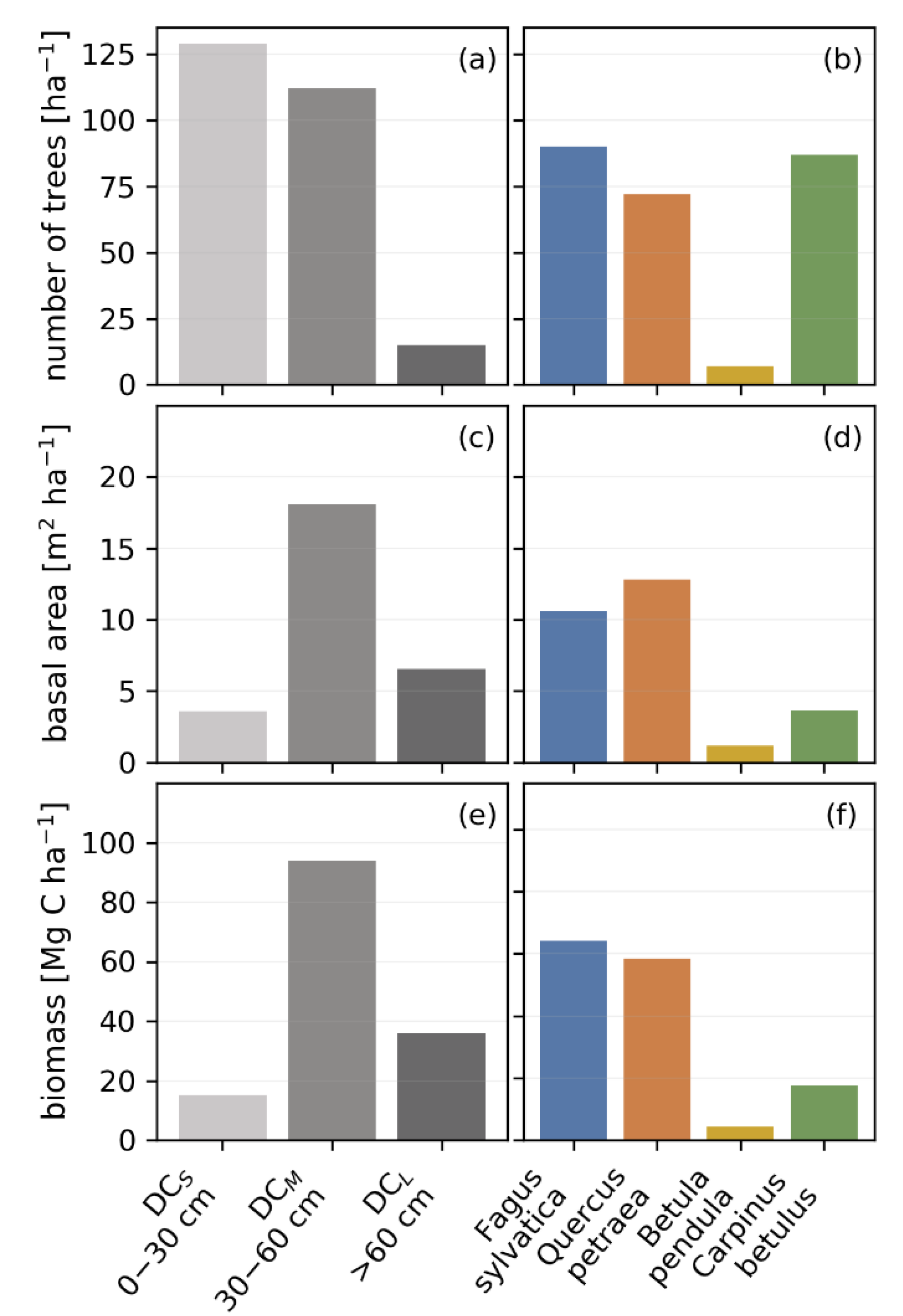
3.1. Biomass, Stem Size, Basal Area and Species Distribution Derived from Inventory Data

Simulations were all initialized with the 1-ha forest inventory data. From this data, we obtained an above-ground carbon content in the biomass of 145 Mg C ha−1, a basal area of 28.2 m2 ha−1 and a stem number per hectare of 260 ha−1 (Figure 1), which were more or less stable during simulation time (2015–2017). The inventory data shows a high proportion of Fagus sylvatica and Quercus petraea in biomass (44.3% and 40.4%, respectively, Figure 1f), stem number (36.2% and 27.7%; respectively, Figure 1b) and basal area (37.6% and 45.3%, respectively; Figure 1d). Carpinus betulus has a relatively large number of small trees (90% of all Carpinus betulus trees) which is typical as this species grows in forest gaps. The smallest proportions in biomass (3%), basal area (4.2%) and in stem number (2.7%) were seen in the species Betula pendula.
Most trees are found in the smallest size class (<30 cm). The number of trees per diameter class decreases with increasing tree size (DCs = 51.2%, DCM = 43%, DCL = 5.8%, Figure 1a). The biomass and basal area per tree size group is highest for the mid-tree size group (64.8% and 64.0%, respectively, Figure 1c,e) and lowest for the smallest tree size group with 10.4% of the total biomass and 12.8% of total basal area.

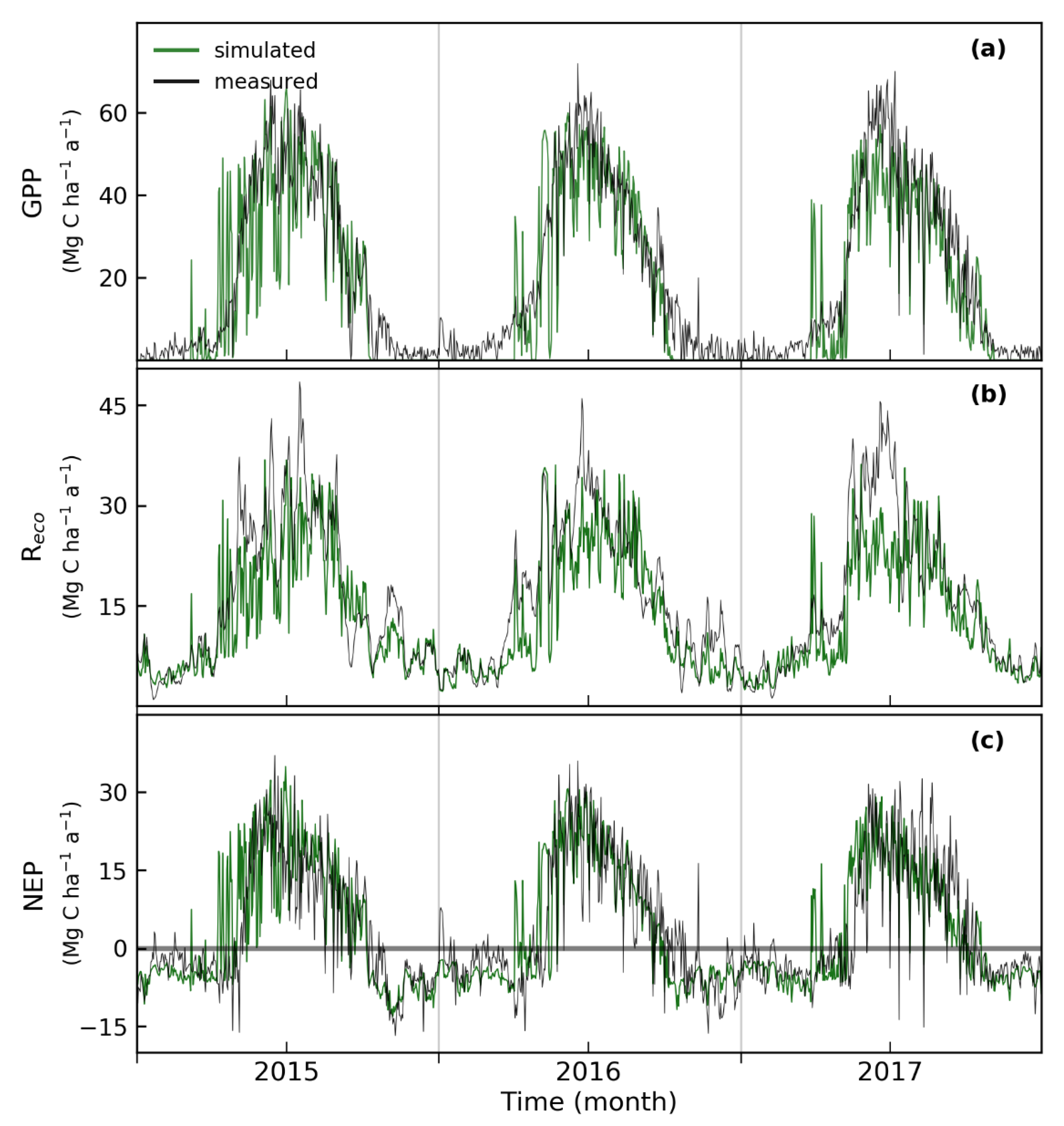
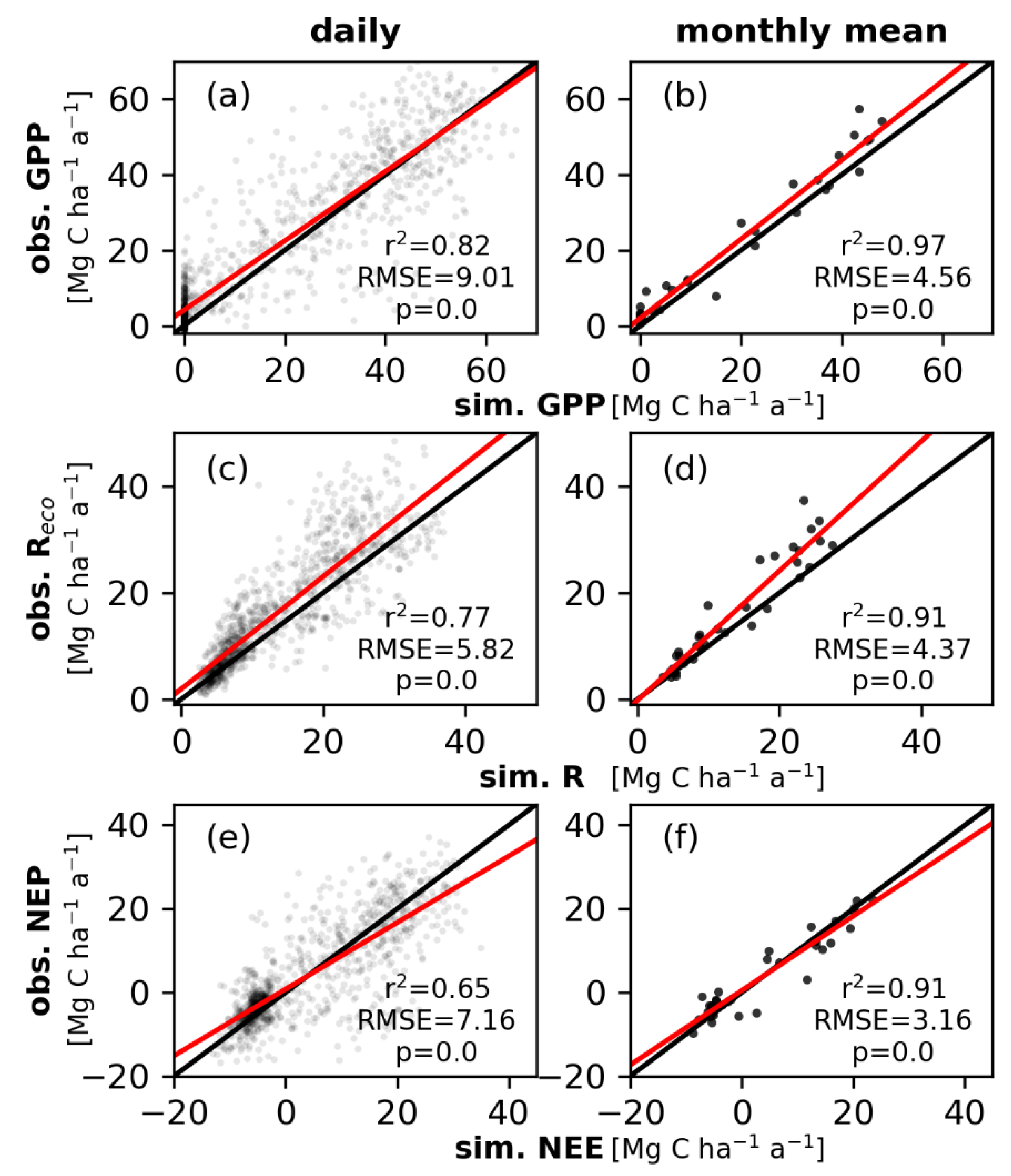
3.2. Simulated and Observed Daily Carbon Fluxes

Simulated and measured daily carbon fluxes for 2015–2017 of the study site DE-HoH are shown in Figure 2. The model can reproduce the measured fluxes at daily time scale and correlates with an R2 of 0.82 for GPP and of 0.77 for Reco. NEP correlates with an R2 of 0.65 (see Figure A2 in Appendix C). In the simulation, we obtain a mean value of 16.6 Mg C ha−1 a−1 for GPP and 13.2 Mg C ha−1 a−1 for Reco. Therefore, the forest is a carbon sink with a mean NEP of 3.4 Mg C ha−1 a−1 (Figure 2). Mean simulated annual values deviate from observed values by 14% for GPP and 17% for Reco. The observed RMSE of daily GPP is 9 Mg C ha−1 a−1 and the RMSE of daily Reco is 5.8 Mg C ha−1 a−1. Simulation results slightly underestimated observed values. However, the magnitude of seasonal and daily fluctuations could be reproduced with our simulation. Measured as well as simulated GPP reaches maximum daily values of around 70 Mg C ha−1 a−1 in summer time. This seasonal course can also be observed in Reco. During summer time Reco reaches maximum values of around 45 Mg C ha−1 a−1. During winter time, when the forest is nearly leafless, the forest releases carbon (−3.9 Mg C ha−1 a−1), and gains carbon in summer (10.8 Mg C ha−1 a−1).
In measured data, daily fluctuations are less compared to simulation results. Fluctuations of simulated carbon fluxes were mainly driven by temperature and water stress as well as by the available incoming light. Non-optimal meteorological conditions have stronger impacts on simulated carbon fluxes whereas measured carbon fluxes show less fluctuations on the daily timescale. One reason might be that sub-daily time scale processes such as stomatal closure to prevent transpiration on days with high temperatures are not directly included in the model. These processes could have influence on daily fluctuations due to a buffer effect for water or temperature stress. On the other hand, the reliable implementation of stress functions, especially the short-term temperature stress response of trees, is partly uncertain.
The strongest differences between simulated and measured values can be observed in spring time at the start of the growing season. During this season, simulated GPP and NEP are higher and fluctuate more than the EC-derived carbon flux. In winter time (October–March), measured GPP (3.7 Mg C ha−1 a−1) differs from model simulations as simulation results show no productivity during the dormant phase in winter time (further discussion on this issue see Appendix E).
Reco could be reproduced with model simulation throughout the year. Deviations between modelled and measured fluxes were mostly observed in summer time on days with high temperatures, low soil water content or on bright days. On these days’ simulated respiration is often lower than the measured respiration.

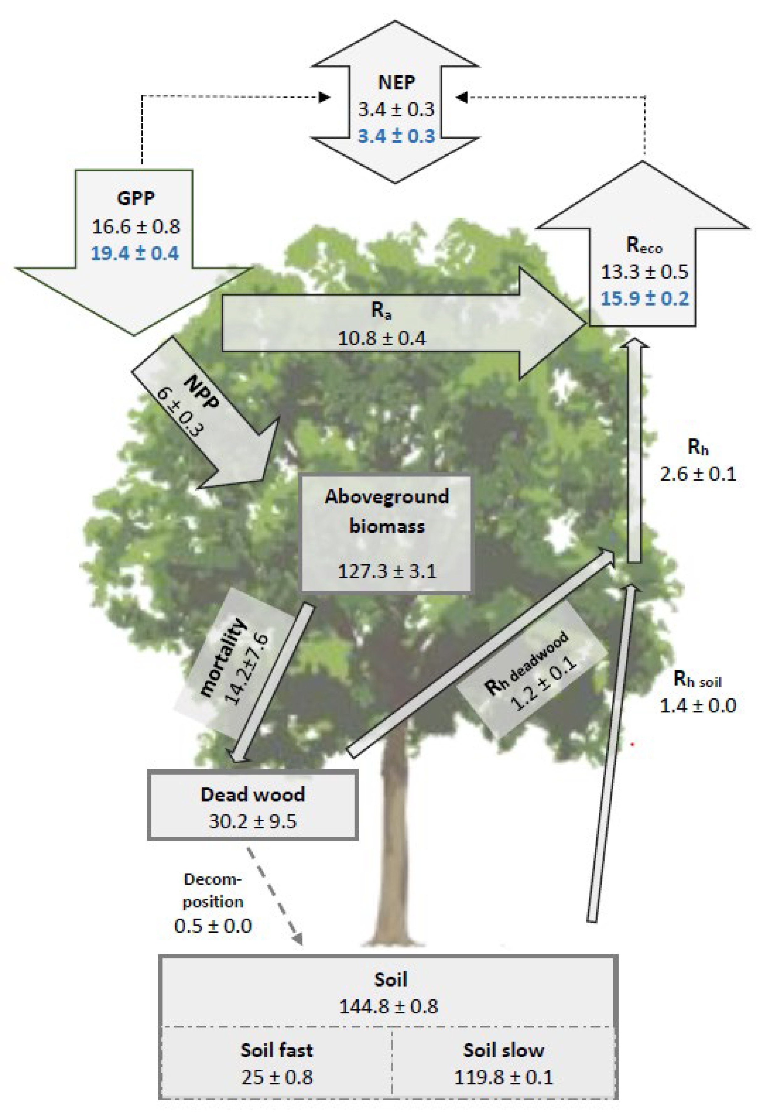
3.3. The Simulated Full Carbon Balance of a Temperate Mixed Deciduous Forest

With the forest model we are able to estimate all major carbon fluxes of the studied forest (including GPP, Reco, NEP, net primary productivity (NPP), Ra, Rh, dead biomass, soil), which are illustrated in Figure 3 as annual averages for the years 2015–2017. The carbon fluxes are related with the three major carbon pools: aboveground biomass, soil carbon and the deadwood pool. Simulations for the test site DE-HoH show that aboveground biomass is the largest carbon pool with around 127.3 Mg C ha−1 and includes foliage as well as the wood components. The simulated deadwood pool (tree mortality) has a carbon content of 30.2 Mg C ha−1. Due to simulated stochastic mortality events, this pool is highly variable throughout the simulation time (±9.5 Mg C ha−1). The total simulated soil carbon stock (144.8 Mg C ha−1) accumulates in two separated pools: the fast- and the slow-decomposition carbon pool. Due to decomposition, both the simulated deadwood pool (Rh deadwood: 1.2 Mg C ha−1 a−1) and the simulated soil carbon pool (Rh soil: 1.4 Mg C ha−1 a−1) also emit carbon through heterotrophic respiration (Rh) into the atmosphere. The simulated GPP of this forest stand is 16.6 Mg C ha−1 a−1 and NPP is 6 Mg C ha−1 a−1. Reco is 13.3 Mg C ha−1 a−1. The forest site De-HoH is therefore a carbon sink throughout the simulation time with a net uptake of 3.4 Mg C ha−1 a−1 (NEP).

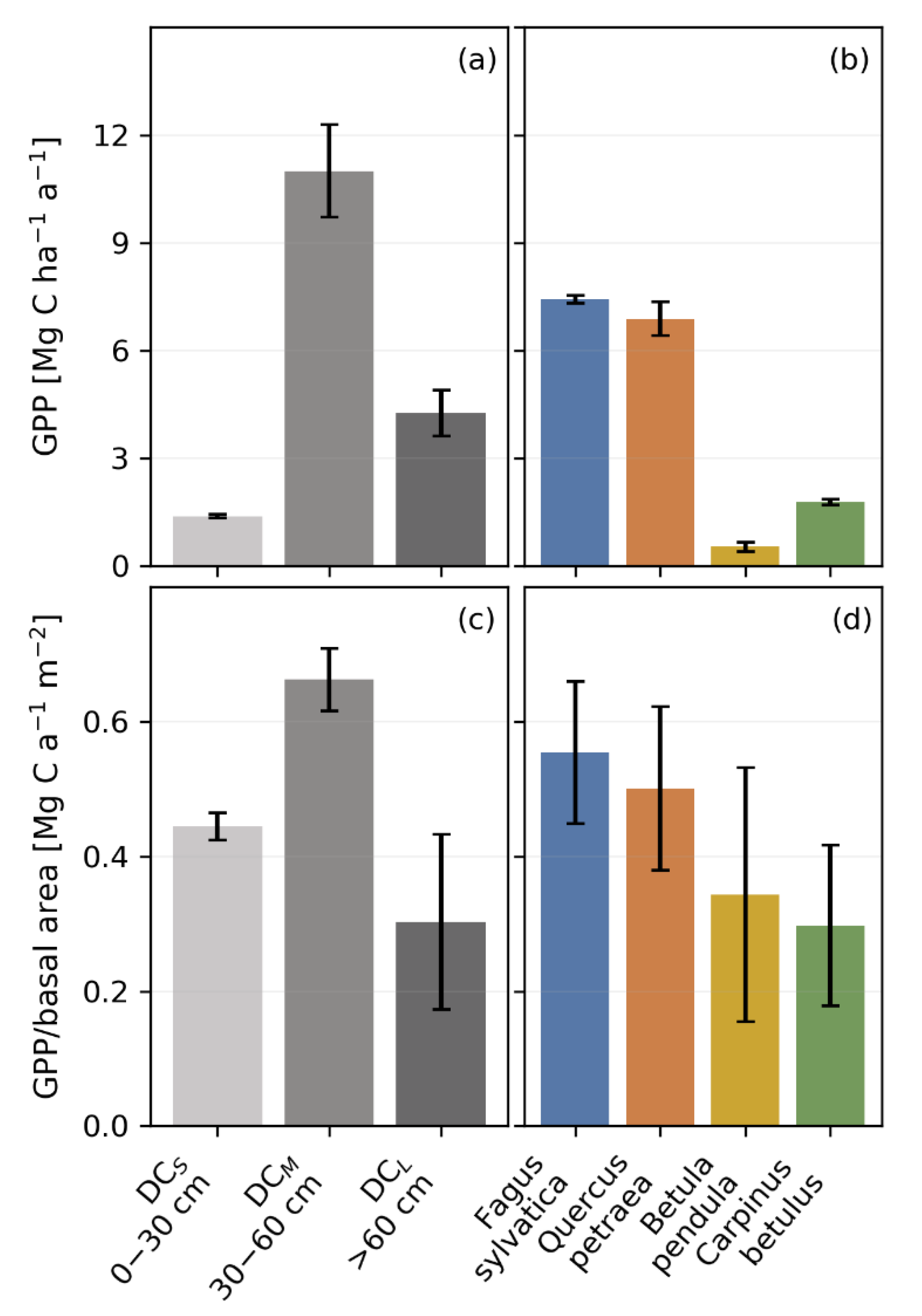
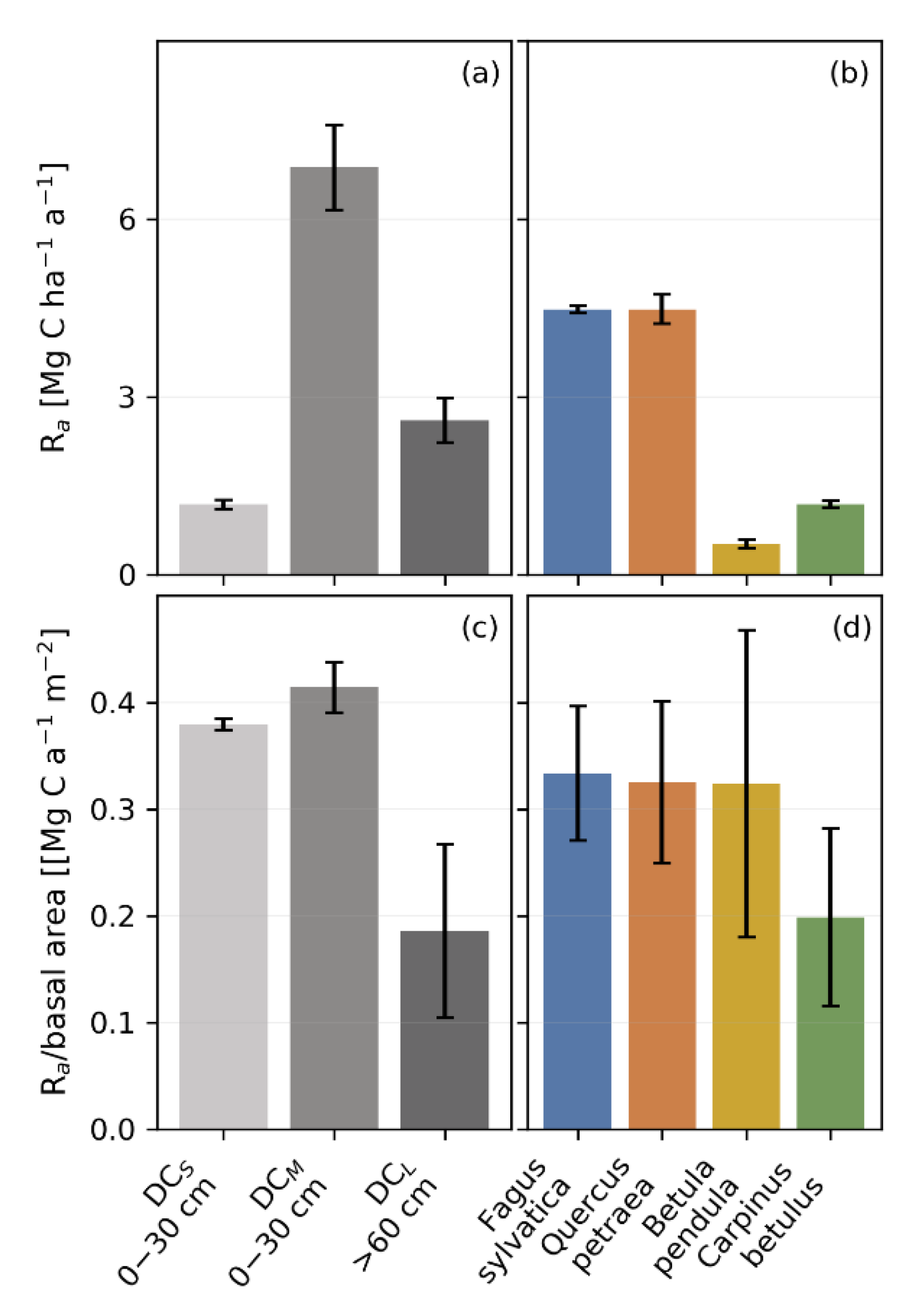
3.4. Productivity and Autotrophic Respiration across Tree Size Classes Derived from Model Simulation

Simulation results show that all mid-sized trees (DCM) have the highest proportion of the simulated mean GPP, with around 66%, and Ra, with nearly 64% (see Figure A3 for respiration), whereas the small trees (DCs) have the lowest share of 8.3% of GPP (see Figure 4a) and 11.1% of Ra. Compared to DCs, trees of the DCL contribute 17.3% more to the overall productivity. This distribution is related to the basal area distribution at the study site (see Figure 1). Therefore, we use the basal area productivity index (see Section 2.6) to compare the relative productivity of each size class based on model simulation results. This comparison shows that the large trees (DCL) have a relative low AGPP of 0.3 Mg C m−2 a−1, while the less-productive small trees (DCs) have a higher AGPP of 0.45 Mg C m−2 a−1 (Figure 4c). The highest production per basal area of 0.66 Mg C m−2 a−1 could be observed in the mid-size tree group. The respiration per area AR is nearly the same for the trees in the DCs and DCM groups by around 0.4 Mg C m−2 a−1, while the large trees have a relatively small respiration index of 0.18 Mg C m−2 a−1 (for respiration see Appendix D, Figure A3).

3.5. Productivity and Autotrophic Respiration across Species Derived from Model Simulation

The distribution of the overall simulated productivity across the four tree species corresponds with the observed species occurrence at the study site, with Fagus sylvatica and Quercus petraea as the dominant tree species in GPP and respiration (Figure 4b, for respiration see Figure A3). In the case of Fagus sylvatica, simulated productivity is 7.4 Mg C ha−1 a−1 with an average AGPP of 0.55 Mg C m−2 a−1. Mean simulated respiration is around 4.4 Mg C ha−1 a−1 which results in an AR of 0.33 Mg C ha−1 a−1. For Quercus petraea, a slightly lower productivity (6.8 Mg C ha−1 a−1) but an equal respiration of 4.4 Mg C ha−1 a−1 were derived. AR of Quercus petraea is nearly the same to that of Fagus sylvatica, whereas the AGPP is lower (0.5 Mg C ha−1 a−1). The mean simulated productivity and respiration of Betula pendula and Carpinus betulus are much lower compared to Fagus sylvatica and Quercus petraea. They contribute only up to 14% of total productivity and 16% of respiration, whereas Betula pendula has the least share of productivity (3.2%) and respiration (4.9%) at this study site. This order can also be seen in productivity and respiration per BA (for respiration see Appendix D and Figure A3) based on model simulation results. Carpinus betulus has an AGPP of 0.3 Mg C m−2 a−1 and an AR of 0.19 Mg C m−2 a−1 whereas Betula pendula has an AGPP of 0.34 Mg C m−2 a−1 and an AR of 0.32 Mg C m−2 a−1 (Figure 4d).

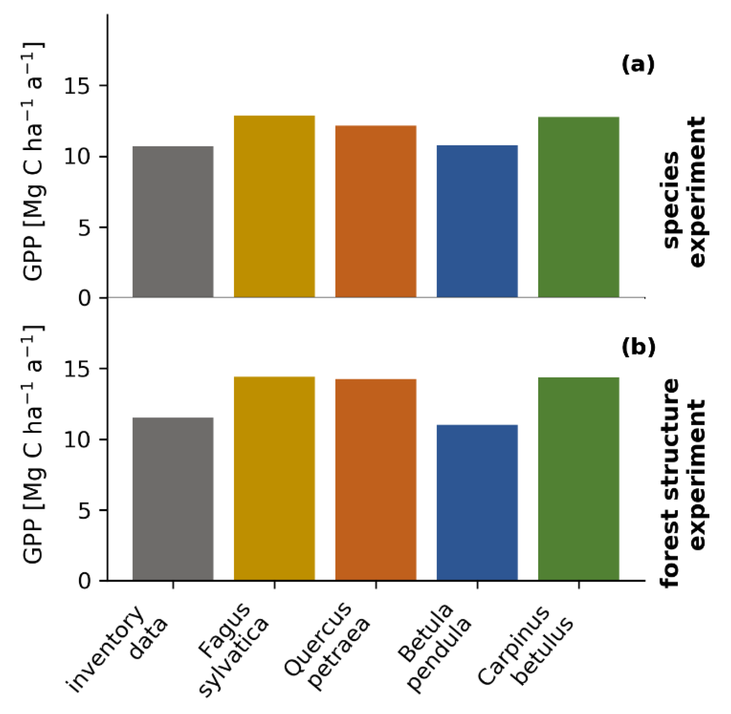
3.6. Virtual Experiments: The Influence of Species Composition and Forest Structure on Forest Productivity

Simulation results of the species experiments show that the productivity for medium-sized trees is almost identical for all four monoculture settings (Figure 5a). For each monoculture setting, independent of the species, productivity of medium sized trees is around 12 Mg C ha−1 a−1. Compared to the inventory data setting, the productivity shows a mean increase of 13.5%. Without large trees (forest structure experiment) productivity of medium-sized trees increased for each simulation run compared to the simulation setting in the species experiment with large trees (Figure 5b). The forest structure experiment based on Quercus petraea benefits the most and shows an increase in productivity of 17.1% compared to the species experiment with Quercus petraea (with large trees). Fagus sylvatica and Carpinus betulus show an increase of around 12%, whereas the simulation based only on trees of the species Betula pendula show nearly no increase in productivity (2%).

4. Discussion

In this study, we demonstrate an approach to simulate daily carbon fluxes with an individual-based forest gap model and provide insights into the productivity and carbon allocation patterns of a mixed temperate forest in Germany. Our main findings from the model simulations are that, first, medium-sized trees account for the largest share of forest productivity at the study site and second, for the investigated forest, stand structure is more important for productivity than species composition.

4.1. Simulated Daily Carbon Fluxes and Uncertainties

Overall, the forest model is capable of reproducing the measured carbon fluxes at the daily time scale as well as the annual and seasonal cycle. Compared with Reco and NEP, GPP is better reproduced in the simulation (for 1:1 plot see Figure A2 in Appendix C), which was also observed in other studies with the same model [41]. One reason for this observation is that Reco is strongly coupled to GPP in FORMIND, and fluctuations in GPP always lead to fluctuations in Reco. Another reason could be that initial soil carbon pools are filled with typical values for German forests (rather than site specific values). Bedrock, management practices, species composition and climate influence soil carbon stocks of an area. In future, study-site-specific measurements of soil carbon stocks should be considered. Another source of uncertainty is based on the EC technique which only measures the net carbon exchange of the ecosystem (NEP) directly while GPP and Reco are derived by partitioning [37,43]. This process includes uncertainties, and values can be different by using other partitioning or post-processing methods whereby a calibration against these fluxes can only be as accurate as the data itself. Additionally, deviations might be a result of the available inventory data that was used to initialize the forest model. This inventory data set is spatially limited to 1 ha and therefore does not cover the whole footprint of the EC tower, which may exceed 10 ha in the main wind direction (for more discussion see Appendix E). Therefore, small deviations of simulated and observed values could have several reasons, from model structure to inventory or measurement uncertainties.

4.2. The Carbon Fluxes of Mixed Temperate Forests

Carbon fluxes of terrestrial ecosystems are highly dependent on management practices and environmental factors such as climate and forest structure. Carbon fluxes of mixed forest with a diverse species composition, e.g., with both evergreen and deciduous trees, are a result of competition between different growth strategies leading to different carbon dynamics. While in Europe temperate humid deciduous forests have typical GPP values of around 13.8 ± 0.5 Mg C ha−1 a−1 and mean Reco values of 10.5 ± 0.6 Mg C ha−1 a−1 (mean biomass:108.8 ± 56.7 Mg C ha−1, mean age: 75 ± 50), evergreen forests (mean biomass: 149.34 ± 135.6 Mg C ha−1, mean age: 91 ± 141) have higher productivity (17.6 ± 0.5 Mg C ha−1 a−1) and respiration rates (13.4 ± 0.6 Mg C ha−1 a−1) [9]. The study of Anderson-Teixeira (2021) reported higher productivity values of 19.5 ± 5.94 Mg C ha−1 a−1 and respiration values of 15.6 ± 7.7 Mg C ha−1 a−1 for mature temperate broadleaf forests (defined as ≥100 years old, biomass 121 ± 34 Mg C ha−1) around the world [44].
Europe-wide studies reported typical values for GPP of 11.1 ± 3.5 Mg C ha−1 a−1 based on EC measurements and site studies (12 ± 0.8 Mg C ha−1 a−1) [45]. Simulated GPPs with process-based ecosystem models such as LPJ-DGVM, Biome-BGC and ORCHIDEE reach mean values from 9 ± 2.3 up to 11.8 ± 2.9 Mg C ha−1 a−1. These Europe-wide estimates include less productive biomes such as Mediterranean, boreal as well as temperate semiarid evergreen forests [9,45], which could explain the lower values compared to temperate humid forests such as DE-HoH. Furthermore, the study site DE-HoH is located in an area with a high nutrient supply, which might lead to a higher productivity compared to other forests with equal species mixing due to favourable growing conditions. Other potential factors are climatic conditions. An evaluation of a global carbon flux dataset has shown that climatic conditions alone are responsible for 71% of global GPP variability, with increasing productivity along with increasing temperature and precipitation [9].
NEP show less correlation with meteorological drivers. Only 5% of the global variability can be explained with temperature and precipitation patterns [9]. NEP derived for EC sites was estimated to be around 3.1 ± 0.3 Mg C ha−1 a−1 for temperate humid deciduous forests with higher values for evergreen forests (+0.87) [9].
For eddy flux sites in Germany, NEP was estimated to be between 4.8–5 Mg C ha−1 a−1 for beech stands (unmanaged, uneven-aged mixed beech stand in mature state (0–250 years old) as well as a managed even-aged beech stand of Fagus sylvatica, 70–150 years old) [46] and between 4.4–6.98 Mg C ha−1 a−1 for a spruce forest [47]. A worldwide study estimated a value of 3.09 ± 1.9 Mg C ha−1 a−1 for mature temperate broadleaf forests (defined as ≥100 years old) [44]. These findings go along with the obtained values in this study and support the observation that European, as well as German forests, continuously accumulate carbon in their biomass and act as carbon sinks [5,9].
Simulation results from this study for Rh are close to literature ranges for similar biomes with slightly lower values compared to literature: values for humid temperate forests are between 3.8–4.2 Mg C ha−1 a−1 for Rh and between 6.7–9.5 Mg C ha−1 a−1 for Ra with higher values in evergreen forest compared to deciduous forest [9]. This might be a result of different species and growth strategies. While deciduous trees accumulate most of the carbon into their woody biomass, evergreen forests accumulates only 70% of their NEP into their woody components. The remainder accumulates into soil and other carbon pools, which often have shorter residence time, leading to higher respiration rates of soil carbon pools [9]. Hence, carbon pools in forest ecosystems depend on species composition and management history.
With increasing forest-structure complexity, e.g., due to a high number of coexisting species and heterogeneous tree age [48], the uncertainty in carbon flux estimates increases as well. Mixed forests need intensive and long-term investigation and monitoring to capture the different patterns within a forest, e.g., light conditions, resource availability, and inter- and intraspecific competition and their influence on the carbon dynamics [10,49]. This complexity is one of the main reasons why mixed forests are less represented in present studies [27]. Forest models can help to reduce this research gap.

4.3. The Impact of Tree Size and Forest Structure on Forest Productivity

Simulation results in this study show an increase of productivity with tree size from small- to medium-size trees, while the productivity of large tress (>60 cm) decreases. These results fit to previous studies, which reported a hump-shaped relationship of growth with tree diameter [50,51] as well as an age-related decline in forest productivity after maturity [11,52]. The age-related decline of productivity might be a result of decreased hydraulic conductance with tree height [11,53]. Therefore, large trees respond with an earlier stomatal closure to prevent a breakdown of the hydraulic system, which reduces daily net photosynthesis [54]. This phenomenon is reported for several tree species [55,56,57,58]. To compensate the higher hydraulic resistance, large trees allocate more carbon into fine roots and stem growth than in leaves, which results in reduced growth efficiency with age [53,59]. Other studies show that large trees can overcome this decline in growth efficiency by an increase of leaf area [60]. Fostering trees with a probable high productivity, e.g., through selective management, does not automatically result in increasing stand productivity because competition and age-related mortality might increase carbon losses. However, small trees with diameters less than 30 cm tend to be relatively less productive (in relation to their leaf area), especially if they are shaded by larger trees [51]. These shaded trees might not receive enough light to grow into the canopy and remain small or even die. Therefore, stand productivity is dependent on vertical stand structure and light conditions. When large trees were excluded from the simulation (virtual experiment), productivity of medium size trees increased. Due to their high productivity, medium size trees play thus an important role for climate mitigation strategies.

4.4. Forest Productivity for Different Tree Species

Despite tree size, species diversity can influence productivity in forest ecosystem by facilitation or complementary resource usage due to e.g., differences in root architecture or differences in their seasonal leaf development [61,62]. However, without resource limitation, species diversity is less important for productivity, which often applies for temperate forests [63]. Plots in Germany with low species diversity and a high occurrence of beech trees showed even higher productivity compared to plots with a higher species diversity [64]. Nevertheless, we found no evidence in the model simulations that one species is more productive than the others. With our model simulation for the investigated forest ecosystem, all species benefit equally from a potential monoculture setting and even more from the removal of large trees. Modelling studies that include evergreen trees could yield different results (Section 4.2). Recent studies mainly focused on information about functional diversity by integrating plant functional types [65] or trait distribution [66] to represent carbon dynamics rather than stand structure. Our virtual model experiments showed that stand structure is an important component in the carbon flux dynamics and should therefore be considered in modelling studies. Especially in heterogeneous forest, the influence of small and medium sized trees on the total stand productivity should not be underestimated. Because of their number and growth efficiency, they can overall be more productive than a few larger trees.

4.5. The Benefit of Modelling Forest Carbon Fluxes

The ability to simulate carbon allocation and pools of a heterogeneous forest using an individual- and process-based forest model with a species-specific parametrisation allows a broad range of analyses and virtual experiments. Such an analysis cannot be done with EC or inventory data alone, especially with regard to mixed forests.
While field measurements are often limited in space or time, forest models can be applied to multiple sites as well as across larger areas and allow for a variety of applications, such as the analysis of intra- and inter-annual carbon cycles of forest ecosystems. In particular, individual-based forest models are relevant tools as they enable the investigation of stand attributes or processes such as carbon dynamics, from local (tree, plot) and short temporal scales (day) up to stand and long temporal scales (years to centuries). This can help to examine the effect of inter- and intra-species competition, species mixing and individual tree growth as well as the effect on stand level. For example, one can analyse the influence of microclimate in a forest on carbon dynamics or the influence of species-specific water use strategies and how this might affect the water cycle due to changes in interception, precipitation or soil water content [27,67] Individual-based models based on forest inventories including tree size as well as species composition with a species-specific parametrisation enables a transfer to other sites. This approach could also facilitate large-scale analysis of carbon flux dynamics on tree level by linking model simulations with remote sensing (e.g., Rödig et al. [68]).
Simulation studies using forest models could help to develop new mitigation strategies based on site specific management plans, e.g., by promoting highly-productive or better-adapted tree species for more resistant forests under extreme events such as droughts [10,48,69]. Virtual experiments with different climates facilitate research on the reactions of different forest compositions and species (mixtures) and how this might change stability, biodiversity or other ecosystem services. These simulation experiments can help to identify important effects on different temporal and spatial scales [27]. The main restriction of forest simulations is the available data for validation and parametrisation, especially for mixed forest stands. This situation might change in the future with new long-term experiments and monitoring sites as well as more available inventory data of mixed forest [70].

5. Conclusions

In this study, we used an individual-based forest gap model in combination with inventory data to investigate daily carbon fluxes of a mixed deciduous forest in Germany at the study site Hohes Holz. We showed that the forest model is capable of reproducing daily carbon fluxes (GPP, Reco, NEP) measured with the EC approach at the study site. In addition, we used the forest model to analyse the role of tree size and species composition for the overall stand productivity. Our model simulation results indicate that medium-sized trees (30–60 cm) account for the largest share (66%) of the total stand productivity at the study site. Virtual experiments show that the exclusion of large trees from the simulation has a stronger effect on simulated productivity than modifying species composition. For this forest, stand structure has at least as much influence on productivity as species diversity. As a conclusion, we recommend considering more information about stand structure in addition to species diversity in modelling studies to decrease uncertainties of carbon dynamic representation and predictions of climate change impacts. We conclude that forest modelling can help to investigate components of the carbon cycle that could not be analysed with EC measurements or traditional forest inventories alone.

Author Contributions

Conceptualization, A.H. (Anne Holtmann) and R.F.; Data curation, A.H. (Anne Holtmann), F.P. and C.R.; Formal analysis, A.H. (Anne Holtmann); Funding acquisition, C.R. and R.F. through the MOMENT phd project; Investigation, A.H. (Anne Holtmann); Methodology, A.H. (Anne Holtmann) and R.F.; Project administration, C.R. and R.F.; Resources, A.H. (Anne Holtmann), A.H. (Andreas Huth), F.P., C.R. and R.F.; Software, A.H. (Anne Holtmann), A.H. (Andreas Huth) and R.F.; Supervision, A.H. (Andreas Huth), C.R. and R.F.; Validation, A.H. (Anne Holtmann); Visualization, A.H. (Anne Holtmann); Writing—original draft, A.H. (Anne Holtmann); Writing—review & editing, A.H. (Anne Holtmann), A.H. (Andreas Huth), F.P., C.R. and R.F.; All authors have read and agreed to the published version of the manuscript.

Funding

This research received no external funding.

Data Availability Statement

FORMIND can be downloaded from www.formind.org (accessed on 24 March 2021). The inventory data presented in this study can be downloaded from: http://www.ufz.de/record/dmp/archive/11178/de/ (accessed on 24 March 2021). The simulation data can be downloaded from: http://www.ufz.de/record/dmp/archive/11181/de/ (accessed on 24 March 2021).

Acknowledgments

We highly appreciate the Computational Hydrosystems’ field crew efforts for keeping the continuous measurements running and performing the forest inventory. We would like to thank the reviewers for their thoughtful comments and efforts towards improving the manuscript.

Conflicts of Interest

The authors declare no conflict of interest.

Appendix A. Measured Variables at the EC Tower

Figure A1. Daily measured (a) air temperature (T) in °C, (b) measured and simulated soil water content (SWC) in % and (c) photon flux density (PPFD) in μmol(photon) m2 s−1 for 2015–2017 at the forest site Hohes Holz. Grey dots in (a,c) represent daily averages. The black lines (a,b) show running means of each variable (7 days). Temperature, precipitation and PPFD serve as input data for the forest model. In the FORMIND model the soil water content is computed per 20 m × 20 m patch and depends on precipitation, interception and run-off as well as on trees individual consumption (transpiration). The simulated soil water is slightly lower than the measured soil water content during winter time (b) and higher during drought events, e.g., in 2016.
Forests 12 00726 g0a1
Table A1. Main abiotic variables measured at the EC tower in 33 m (air temperature), and 49 m (radiation and precipitation), and in 0.4 m soil depth (soil moisture) needed as input for the forest model FORMIND.
Variable MeasuredAbbreviationUnitInstrument Type, Manufacturer
global radiationSWD
SWDR
W m−2CNR4, Kipp & Zonen, Delft, The Netherlands
NR01, Hukseflux, Delft, The Netherlands
photosynthetic photon flux densityPPFDµmol (photons) m−2 s−1LI-COR, Lincoln, NE, USA
air temperatureTair°C/KHMP155, Vaisala, Helsinki, Finnland
precipitationprecip
precip_back
mmThies 5.4032.35.008, Adolf Thies GmbH & Co. KG, Göttingen, Germany
Thies 54000, Adolf Thies GmbH & Co. KG, Göttingen, Germany
soil water contentSMVol.%CS616, 30cm length, Campbell Scientific, Shepshed, UK

Appendix B

Appendix B.1. The Carbon Flux Module

The carbon cycle in FORMIND is simulated using four separate carbon pools: the aboveground biomass pool, the deadwood pool (D in Mg C ha−1), the fast (Sfast in Mg C ha−1) and the slow (Sslow in Mg C ha−1) decomposing soil pool [29]. The input to the deadwood pool is driven by tree mortality (M in Mg C ha−1 a−1). Microorganisms decompose the deadwood to soil with a specific degradation rate. The rate of decomposing defines if it accumulates into the slow ( t D S s l o w ) or fast ( t D S f a s t ) carbon soil stock (in Mg C ha−1 a−1). Due to decomposition, the deadwood pool ( t D A in Mg C ha−1 a−1) and both soil carbon pools ( t S s l o w A , t S f a s t A in Mg C ha−1 a−1) also emit carbon into the atmosphere. The change in the pools are calculated as follows:
d D d t = M ( t D A + t D S s l o w + t D S f a s t ) · D
d S s l o w d t = t D S s l o w · D t S s l o w A · S s l o w
d S f a s t d t = t D S f a s t · D t S f a s t A · S f a s t
To calculate the total ecosystem respiration (Reco in Mg C ha−1 a−1), the soil and deadwood respiration (Rh in Mg C ha−1 a−1) has to be added to the sum of respiration over all trees (Ra in Mg C ha−1 a−1).
R h = t D A · D + t S s l o w A · S s l o w + t S f a s t A · S f a s t
R a = R m + R g
R e c o = R a + R h
The ecosystem GPP (Mg C ha−1 a−1) is the sum of GPPtree of all simulated trees. A fraction of the GPP is respired back into the atmosphere via autotrophic respiration Ra which can be divided into maintenance respiration (Rm in Mg C ha−1 a−1) for the maintenance of living cells and growth respiration (Rg in Mg C ha−1 a−1) for the net gain of biomass. The difference between GPP and Ra is NPP (net primary productivity, in Mg C ha−1 a−1) of foliage, stem, roots, branches and other plant organs. The metabolism of dead organic matter by microbes leads to heterotrophic respiration (Rh in Mg C ha−1 a−1) into the atmosphere. The sum of Rh and Ra is the total terrestrial ecosystem respiration (Reco). The difference between GPP and Reco is the net ecosystem productivity (NEP in Mg C ha−1 a−1). A positive NEP indicates the ecosystem as a carbon sink:
N E P = G P P R e c o

Appendix B.2. Tree Photosynthesis

The potential GPPtree (in Mg C ha−1 a−1) for one tree is calculated on the leaf level using a light-response function and is then integrated over the entire canopy [40]. The light availability for each tree is based on the individual light climate (i.e., shading) and the photosynthetically active period defined by day length and vegetation period. Climatic input variables are used to calculate reduction factors of potential GPP due to a reduced soil water content or temperature stress.
Without any reduction (under optimal climate conditions) the potential GPPtree of a tree is:
G P P t r e e ( I i n d ( P P F D ( t ) ) ) = p m a x k l n { α k I i n d ( P P F D ( t ) ) + p m a x [ 1 m ] α k I i n d ( P P F D ( t ) ) e k L A I + p m a x [ 1 m ] } A c ψ
where p m a x is the species-specific maximum photosynthetic rate (μmol(CO2) m−2 s−1) of the tree species, α is the species-specific initial slope of the light-response curve (μmol(CO2) μmol(photons)−1), k is the light extinction factor and m is the transmission coefficient of the leaves. Iind is the fraction of the PPFD at daily time step t that reaches the top of the individual tree. Ac (m2) is the crown area, and ψ the photosynthetically active period of the time scale.
Under climate stress conditions, GPPtree can be reduced due to a limited available soil water content and due to temperature dependency [41]. The reduction of GPP is expressed through a reduction factor φ S W ( t ) (0, 1) for temperature and φ S W (0, 1) for water stress:
G P P t r e e = G P P p t r e e ( t ) · φ S W ( t ) · φ T ( t )
The temperature reduction factor is calculated by the following normal distribution function based on Topt, an optimal temperature without reduction, and Tsig, which defines the range of temperatures distributed around Topt with nearly no reduction [41]:
φ T ( t ) = e ( T ( t ) T o p t T s i g ) n
Water deficit influences the potential photosynthesis negatively when the soil water content is below the available soil water content for the trees ( S W m w s which can be calculated through the S W p w p and the S W f c of the soil [71].
S W m s w = S W p w p + 0.4 ( S W f c S W p w p )
S W m s w defines the minimum soil water content with no reduction, therefore the reduction factor φ S W is calculated as followed [41]:
φ S W ( t ) = { 0 : S W ( t ) < S W p w p S W ( t ) S W p w p S W m w s S W p w p : S W p w p < S W ( t ) < S W m w s 1 : S W ( t ) > S W m w s
The soil water content (SWC) is calculated using the daily sum of incoming precipitation, interception by leaves, transpiration of trees, and above- as well as below-ground water runoff.

Appendix B.3. Tree Respiration

The respiration of each tree (Ra) is partitioned into maintenance respiration (Rm) and growth respiration (Rg). The maintenance respiration is calculated proportionally to the existing biomass of a tree, and is limited by a factor dependent on air temperature κ ( T ) .
R m ( t ) = r m B ( t ) κ ( T ( t ) )
Between maintenance respiration and temperature an exponentially relationship is assumed and expressed in the following equation, where Q10 and Tref are constant:
κ ( T ( t ) ) = Q 10 T ( t ) T r e f 10
The growth respiration (Rg) is a constant fraction of (GPP-Rm) proportional to the growth rate of a tree.

Appendix C. Model Parameter

Model Parameter Calibration

The Parameterization for the species-specific allometric relationships between biomass and dbh as well as between dbh and height, crown diameter and mortality rate for Fagus sylvatica, Quercus petraea and Betula pendula are based on Bohn et al. [30] (Table A3) except for pmax and α (Table A2). The parameterization for Betula pendula was also taken for Carpinus betulus due to equal growth strategies.
All adjusted parameters (Table A2) were calibrated against measured NEP, GPP and Reco. The productivity parameters pmax and α needs to be adjusted upwards compared to Bohn 2014 to reach the measured carbon fluxes. The parameters that are influencing the carbon fluxes based on climate variability such as Topt, Tsig, Q10, Tref and the water stress related parameters SWpwp, SWfc were calibrated against filtered EC fluxes for optimal climate condition according to Rödig et al. [41]. Model functions were directly fitted through filtered data.
Other soil parameters such as porosity and pore size distribution. where set according [31] classification of a silt loam soil type.
Table A2. Calibrated Model Parameter.
ParameterFagus sylvaticaQuercus petraeaBetula pendulaCarpinus betulus
Productivity
pmaxmax. photoproducitvity of leaf (µmol (CO2) s−1 m−2)15.76820.24422.67215.768
αslope of light response curve (µmol (CO2) µmol(photons)−1)0.12880.07360.07280.1288
Temperature
Toptoptimal temperature for photosynthesis (°C)20.8
Tsigwidth of new temperature curve (°C)10.1
Q10constant for temperature-dependent respiration2.12
TrefReference temperature (°C)18.4
Water
SWpwppermanent wilting point (vol-%)7.8
SWfcfield capacity (vol-%)25.8
ksFully saturated conductivity ms−10.0000061
klInterception contant0.1
psPore size distribution0.105
porPorosity of the soil (vol-%)50.1
SWInitInitial soil water content (vol-%)22.24
ΘrResidual soil water content (vol-%)1.5
Establishment
NseedsNumber of global seeds per ha−1 a−1 (estimated)18121018
Figure A2. Daily (left, (a) GPP, (c) Reco, (e) NEP) and monthly (right, (b) GPP, (d) Reco, (f) NEP) mean simulated vs. observed ecosystem carbon fluxes (NEP, GPP and Reco) at Hohes Holz for the calibrated parameterization for three years (2015–2017).
Forests 12 00726 g0a2
The forest model is capable to reproduce the measured GPP at Hohes Holz at the daily (r2 = 0.82, RMSE = 9.01) and even better on the monthly timescale (r2 = 0.97, RMSE = 4.56). The simulated respiration correlates with the measured values with an r2 of 0.77 (RMSE = 5.82) on the daily timescale and with an r2 of 0.91 (RMSE = 4.37) on the monthly timescale. NEP is reproduced on the monthly timescale with an r2 of 0.91 and a RMSE of 3.16. On the daily timescale NEP correlated with an r2 of 0.65 (RMSE = 7.16).
Table A3. Summary of the species-specific parameters taken from Bohn (2014) [30].
ParameterFagus sylvaticaQuercusBetula spp.Carpinus betulus
Biomass
b1biomass calculation [72]1.2021.1511.0911.202
b25.7275.1876.3945.727
d1Growth curve [72]4.70 × 10−37.06 × 10−33.74 × 10−34.70 × 10−3
d21.2520.7031.4451.252
d31.391.1841.1451.39
Geometry
l0LAI-dbh relation [73]6.15.45.36.1
l10000
h0Height-dbh relation [72]1.9161.8791.7111.916
h161.03645.34151.48861.036
c1Crown-dbh relation [72]0.1550.1730.2070.155
c20.1250.0541.7600.125
c30.0660.0660.2770.066
f0Form factor-dbh relation0.5710.6310.4990.571
f10.1810.2270.0970.181
Mortality
m0max. mortality at establishment0.008900.006570.048410.0890
m1slope of mortality−0.761−0.950−0.210−0.761
r2[72]0.0010.0020.0180.001
Light and Establishment
kLight extinction factor0.70.70.70.7
mTransmission coefficient of leaves [74]0.10.10.10.1
IminMin. light intensity% to establish [30]0.30.30.30.3

Appendix D. Autotrophic Respiration across Tree Size Classes and Species

Figure A3. Simulated annual mean autotrophic respiration (Ra); (a,b), as well as respiration per basal area (c,d) across three tree size classes and occurring species.
Forests 12 00726 g0a3

Appendix E. Further Discussion: Inventory Data

Some deviation, mainly observed in spring and winter time, are most likely resulting from a model simplification concerning the implementation of the intra-annual cycle of deciduous tree species. Deciduous trees have two seasons: one vegetation period were trees are photo active and one dormant time in winter without photosynthesis at all. This model simplification explains the deviation and absent photosynthesis in winter in simulation results. Though, inventory data does not include a single needle leaf tree we can not exclude that there are some in the footprint area. This could be on explanation for the measured productivity in winter. A larger inventory data set could help to reduce uncertainties regarding the tree species composition. Needle leaf trees in the inventory data would have led to simulated productivity in winter time because simulated vegetation period for needle leaf trees would be a full year (365 days).

References

  1. Fawzy, S.; Osman, A.I.; Doran, J.; Rooney, D.W. Strategies for mitigation of climate change: A review. Environ. Chem. Lett. 2020, 18, 2069–2094. [Google Scholar] [CrossRef]
  2. Bonan, G.B. Forests and Climate Change: Forcings, Feedbacks, and the Climate Benefits of Forests. Science 2008, 320, 1444–1449. [Google Scholar] [CrossRef] [Green Version]
  3. Pan, Y.; Birdsey, R.A.; Fang, J.; Houghton, R.; Kauppi, P.E.; Kurz, W.A.; Phillips, O.L.; Shvidenko, A.; Lewis, S.L.; Canadell, J.G.; et al. A Large and Persistent Carbon Sink in the World’s Forests. Science 2011, 333, 988–993. [Google Scholar] [CrossRef] [Green Version]
  4. Bösch, M.; Elsasser, P.; Franz, K.; Lorenz, M.; Moning, C.; Olschewski, R.; Rödl, A.; Schneider, H.; Schröppel, B.; Weller, P. Forest ecosystem services in rural areas of Germany: Insights from the national TEEB study. Ecosyst. Serv. 2018, 31, 77–83. [Google Scholar] [CrossRef]
  5. Wellbrock, N.; Grüneberg, E.; Riedel, T.; Polley, H. Carbon stocks in tree biomass and soils of German forests. Cent. Eur. For. J. 2017, 63, 105–112. [Google Scholar] [CrossRef] [Green Version]
  6. Friedlingstein, P.; Jones, M.W.; O’Sullivan, M.; Andrew, R.M.; Hauck, J.; Peters, G.P.; Peters, W.; Pongratz, J.; Sitch, S.; Le Quéré, C.; et al. Global Carbon Budget 2019. Earth Syst. Sci. Data 2019, 11, 1783–1838. [Google Scholar] [CrossRef] [Green Version]
  7. Harris, N.L.; Gibbs, D.A.; Baccini, A.; Birdsey, R.A.; de Bruin, S.; Farina, M.; Fatoyinbo, L.; Hansen, M.C.; Herold, M.; Houghton, R.A.; et al. Global maps of twenty-first century forest carbon fluxes. Nat. Clim. Chang. 2021. [Google Scholar] [CrossRef]
  8. Liu, S. Quantifying the spatial details of carbon sequestration potential and performance. In Carbon Sequestration and Its Role in the Global Carbon Cycle; Mcpherson, B.J., Sundquist, E.T., Eds.; American Geophysical Union: Washington, DC, USA, 2009; Volume 183, pp. 117–128. [Google Scholar]
  9. Luyssaert, S.; Inglima, I.; Jung, M.; Richardson, A.D.; Reichstein, M.; Papale, D.; Piao, S.L.; Schulze, E.D.; Wingate, L.; Matteucci, G.; et al. CO2 balance of boreal, temperate, and tropical forests derived from a global database. Glob. Chang. Biol. 2007, 13, 2509–2537. [Google Scholar] [CrossRef] [Green Version]
  10. Shanin, V.; Komarov, A.; Mäkipä, R. Tree species composition affects productivity and carbon dynamics of different site types in boreal forests. Eur. J. For. Res. 2014, 133, 273–286. [Google Scholar] [CrossRef] [Green Version]
  11. Ryan, M.G.; Binkley, D.; Fownes, J.H. Age-Related Decline in Forest Productivity: Pattern and Process. Adv. Ecol. Res. 1997, 27, 213–262. [Google Scholar] [CrossRef]
  12. Keith, H.; Lindenmayer, D.; MacKey, B.; Blair, D.; Carter, L.; McBurney, L.; Okada, S.; Konishi-Nagano, T. Managing temperate forests for carbon storage: Impacts of logging versus forest protection on carbon stocks. Ecosphere 2014, 5. [Google Scholar] [CrossRef] [Green Version]
  13. Mund, M.; Schulze, E.D. Impacts of Forest Management on the Carbon Budget of European Beech (Fagus sylvatica) Forests. Available online: https://www.researchgate.net/publication/42088941_Impacts_of_forest_management_on_the_carbon_budget_of_European_Beech_Fagus_sylvatica_forests (accessed on 19 February 2021).
  14. Vande Walle, I.; Mussche, S.; Samson, R.; Lust, N.; Lemeur, R. The above- and belowground carbon pools of two mixed deciduous forest stands located in East-Flanders (Belgium). Ann. For. Sci. 2001, 58, 507–517. [Google Scholar] [CrossRef]
  15. Teets, A.; Fraver, S.; Hollinger, D.Y.; Weiskittel, A.R.; Seymour, R.S.; Richardson, A.D. Linking annual tree growth with eddy-flux measures of net ecosystem productivity across twenty years of observation in a mixed conifer forest. Agric. For. Meteorol. 2018, 249, 479–487. [Google Scholar] [CrossRef]
  16. Baldocchi, D. Measuring fluxes of trace gases and energy between ecosystems and the atmosphere-the state and future of the eddy covariance method. Glob. Chang. Biol. 2014, 20, 3600–3609. [Google Scholar] [CrossRef]
  17. Schmid, H.P. Source areas for scalars and scalar fluxes. Bound.-Layer Meteorol. 1994, 67, 293–318. [Google Scholar] [CrossRef]
  18. Medvigy, D.; Wofsy, S.C.; Munger, J.W.; Hollinger, D.Y.; Moorcroft, P.R. Mechanistic scaling of ecosystem function and dynamics in space and time: Ecosystem Demography model version 2. J. Geophys. Res. Biogeosci. 2009, 114, 1–21. [Google Scholar] [CrossRef] [Green Version]
  19. Baldocchi, D.; Falge, E.; Gu, L.; Olson, R.; Hollinger, D.; Running, S.; Anthoni, P.; Bernhofer, C.; Davis, K.; Evans, R.; et al. FLUXNET: A New Tool to Study the Temporal and Spatial Variability of Ecosystem-Scale Carbon Dioxide, Water Vapor, and Energy Flux Densities. Bull. Am. Meteorol. Soc. 2001, 82, 2415–2434. [Google Scholar] [CrossRef]
  20. Falge, E.; Baldocchi, D.; Tenhunen, J.; Aubinet, M.; Bakwin, P.; Berbigier, P.; Bernhofer, C.; Burba, G.; Clement, R.; Davis, K.J.; et al. Seasonality of ecosystem respiration and gross primary production as derived from FLUXNET measurements. Agric. For. Meteorol. 2002, 113, 53–74. [Google Scholar] [CrossRef] [Green Version]
  21. Reichstein, M.; Falge, E.; Baldocchi, D.; Papale, D.; Aubinet, M.; Berbigier, P.; Bernhofer, C.; Buchmann, N.; Gilmanov, T.; Granier, A.; et al. On the separation of net ecosystem exchange into assimilation and ecosystem respiration: Review and improved algorithm. Glob. Chang. Biol. 2005, 11, 1424–1439. [Google Scholar] [CrossRef]
  22. Grassi, G.; House, J.; Dentener, F.; Federici, S.; Den Elzen, M.; Penman, J. The key role of forests in meeting climate targets requires science for credible mitigation. Nat. Clim. Chang. 2017, 7, 220–226. [Google Scholar] [CrossRef]
  23. Anderegg, W.R.L.; Trugman, A.T.; Badgley, G.; Anderson, C.M.; Bartuska, A.; Ciais, P.; Cullenward, D.; Field, C.B.; Freeman, J.; Goetz, S.J.; et al. Climate-driven risks to the climate mitigation potential of forests. Science 2020, 368, eaaz7005. [Google Scholar] [CrossRef]
  24. Ceccherini, G.; Duveiller, G.; Grassi, G.; Lemoine, G.; Avitabile, V.; Pilli, R.; Cescatti, A. Abrupt increase in harvested forest area over Europe after 2015. Nature 2020, 583, 72–77. [Google Scholar] [CrossRef]
  25. Shugart, H.H.; Wang, B.; Fischer, R.; Ma, J.; Fang, J.; Yan, X.; Huth, A.; Armstrong, A.H. Gap models and their individual-based relatives in the assessment of the consequences of global change. Environ. Res. Lett. 2018, 13, 033001. [Google Scholar] [CrossRef] [Green Version]
  26. Bugmann, H. A review of forest gap models. Clim. Chang. 2001, 51, 259–305. [Google Scholar] [CrossRef]
  27. Pretzsch, H.; Forrester, D.I.; Rötzer, T. Representation of species mixing in forest growth models: A review and perspective. Ecol. Modell. 2015, 313, 276–292. [Google Scholar] [CrossRef] [Green Version]
  28. Wollschläger, U.; Attinger, S.; Borchardt, D.; Brauns, M.; Cuntz, M.; Dietrich, P.; Fleckenstein, J.H.; Friese, K.; Friesen, J.; Harpke, A.; et al. The Bode hydrological observatory: A platform for integrated, interdisciplinary hydro-ecological research within the TERENO Harz/Central German Lowland Observatory. Environ. Earth Sci. 2017, 76, 29. [Google Scholar] [CrossRef]
  29. Paulick, S.; Dislich, C.; Homeier, J.; Fischer, R.; Huth, A. The carbon fluxes in different successional stages: Modelling the dynamics of tropical montane forests in South Ecuador. For. Ecosyst. 2017, 4, 5. [Google Scholar] [CrossRef] [Green Version]
  30. Bohn, F.J.; Frank, K.; Huth, A. Of climate and its resulting tree growth: Simulating the productivity of temperate forests. Ecol. Modell. 2014, 278, 9–17. [Google Scholar] [CrossRef]
  31. Maidment, D. Handbook of Hydrology; McGrawHill Inc.: New York, NY, USA, 1993; Volume 141, ISBN 9780070397323. [Google Scholar]
  32. Zacharias, S.; Bogena, H.; Samaniego, L.; Mauder, M.; Fuß, R.; Pütz, T.; Frenzel, M.; Schwank, M.; Baessler, C.; Butterbach-Bahl, K.; et al. A Network of Terrestrial Environmental Observatories in Germany. Vadose Zone J. 2011, 10, 955–973. [Google Scholar] [CrossRef] [Green Version]
  33. Aubinet, M.; Grelle, A.; Ibrom, A.; Rannik, U.; Moncrieff, J.; Foken, T.; Kowalski, A.S.; Martin, P.H.; Berbigier, P.; Bernhofer, C.; et al. Estimates of the Annual Net Carbon and Water Exchange of Forests: The EUROFLUX Methodology. Adv. Ecol. Res. 2000, 30, 113–175. [Google Scholar] [CrossRef]
  34. Rebmann, C.; Aubinet, M.; Schmid, H.; Arriga, N.; Aurela, M.; Burba, G.; Clement, R.; De Ligne, A.; Fratini, G.; Gielen, B.; et al. ICOS eddy covariance flux-station site setup: A review. Int. Agrophys. 2018, 32, 471–494. [Google Scholar] [CrossRef]
  35. Fratini, G.; Mauder, M. Towards a consistent eddy-covariance processing: An intercomparison of EddyPro and TK3. Atmos. Meas. Tech. 2014, 7, 2273–2281. [Google Scholar] [CrossRef] [Green Version]
  36. Burba, G.; Anderson, D. Introduction to the Eddy Covariance Method: General Guidelines and Conventional Workflow; LI-COR Biosciences: Lincoln, NE, USA, 2007. [Google Scholar] [CrossRef]
  37. Wutzler, T.; Lucas-Moffat, A.; Migliavacca, M.; Knauer, J.; Sickel, K.; Šigut, L.; Menzer, O.; Reichstein, M. Basic and extensible post-processing of eddy covariance flux data with REddyProc. Biogeosciences 2018, 15, 5015–5030. [Google Scholar] [CrossRef] [Green Version]
  38. Moritz, S.; Bartz-Beielstein, T. Imputets: Time series missing value imputation in R. R J. 2017, 9, 207–218. [Google Scholar] [CrossRef] [Green Version]
  39. Chapin, F.S.; Woodwell, G.M.; Randerson, J.T.; Rastetter, E.B.; Lovett, G.M.; Baldocchi, D.D.; Clark, D.A.; Harmon, M.E.; Schimel, D.S.; Valentini, R.; et al. Reconciling Carbon-cycle Concepts, Terminology, and Methods. Ecosystems 2006, 9, 1041–1050. [Google Scholar] [CrossRef] [Green Version]
  40. Fischer, R.; Bohn, F.; Dantas de Paula, M.; Dislich, C.; Groeneveld, J.; Gutiérrez, A.G.; Kazmierczak, M.; Knapp, N.; Lehmann, S.; Paulick, S.; et al. Lessons learned from applying a forest gap model to understand ecosystem and carbon dynamics of complex tropical forests. Ecol. Modell. 2016, 326, 124–133. [Google Scholar] [CrossRef] [Green Version]
  41. Rödig, E.; Huth, A.; Bohn, F.; Rebmann, C.; Cuntz, M. Estimating the carbon fluxes of forests with an individual-based forest model. For. Ecosyst. 2017, 4, 4. [Google Scholar] [CrossRef] [Green Version]
  42. Grüneberg, E.; Schöning, I.; Riek, W.; Ziche, D.; Evers, J. Carbon Stocks and Carbon Stock Changes in German Forest Soils; Springer: Cham, Switzerland, 2019; pp. 167–198. [Google Scholar]
  43. Campioli, M.; Malhi, Y.; Vicca, S.; Luyssaert, S.; Papale, D.; Peñuelas, J.; Reichstein, M.; Migliavacca, M.; Arain, M.A.; Janssens, I.A. Evaluating the convergence between eddy-covariance and biometric methods for assessing carbon budgets of forests. Nat. Commun. 2016, 7. [Google Scholar] [CrossRef]
  44. Anderson-Teixeira, K.J.; Herrmann, V.; Banbury Morgan, R.; Bond-Lamberty, B.; Cook-Patton, S.C.; Ferson, A.E.; Muller-Landau, H.; Wang, M.M.H. Carbon cycling in mature and regrowth forests globally. Environ. Res. Lett. 2021. [Google Scholar] [CrossRef]
  45. Luyssaert, S.; Ciais, P.; Piao, S.L.; Schulze, E.D.; Jung, M.; Zaehle, S.; Schelhaas, M.J.; Reichstein, M.; Churkina, G.; Papale, D.; et al. The European carbon balance. Part 3: Forests. Glob. Chang. Biol. 2010, 16, 1429–1450. [Google Scholar] [CrossRef]
  46. Anthoni, P.M.; Knohl, A.; Rebmann, C.; Freibauer, A.; Mund, M.; Ziegler, W.; Kolle, O.; Schulze, E.-D. Forest and agricultural land-use-dependent CO2 exchange in Thuringia, Germany. Glob. Chang. Biol. 2004, 10, 2005–2019. [Google Scholar] [CrossRef]
  47. Prescher, A.K.; Grünwald, T.; Bernhofer, C. Land use regulates carbon budgets in eastern Germany: From NEE to NBP. Agric. For. Meteorol. 2010, 150, 1016–1025. [Google Scholar] [CrossRef]
  48. Bravo-Oviedo, A.; Pretzsch, H.; Ammer, C.; Andenmatten, E.; Barbati, A.; Barreiro, S.; Brang, P.; Bravo, F.; Coll, L.; Corona, P.; et al. European mixed forests: Definition and research perspectives. For. Syst. 2014, 23, 518–533. [Google Scholar] [CrossRef]
  49. Pretzsch, H.; Bielak, K.; Block, J.; Bruchwald, A.; Dieler, J.; Ehrhart, H.P.; Kohnle, U.; Nagel, J.; Spellmann, H.; Zasada, M.; et al. Productivity of mixed versus pure stands off oak (Quercus petraea (Matt.) Liebl. and Quercus robur L.) and European beech (Fagus sylvatica L.) along an ecological gradient. Eur. J. For. Res. 2013, 132, 263–280. [Google Scholar] [CrossRef]
  50. Chave, J.; Muller-Landau, H.C.; Baker, T.R.; Easdale, T.A.; Steege, H.; Webb, C.O. Regional and phylogenetic variation of wood density across 2456 neotropical tree species. Ecol. Appl. 2006, 16, 2356–2367. [Google Scholar] [CrossRef] [Green Version]
  51. Caspersen, J.P.; Vanderwel, M.C.; Cole, W.G.; Purves, D.W. How Stand Productivity Results from Size- and Competition-Dependent Growth and Mortality. PLoS ONE 2011, 6, e28660. [Google Scholar] [CrossRef] [PubMed]
  52. Tang, J.; Luyssaert, S.; Richardson, A.D.; Kutsch, W.; Janssens, I.A. Steeper declines in forest photosynthesis than respiration explain age-driven decreases in forest growth. Proc. Natl. Acad. Sci. USA 2014, 111, 8856–8860. [Google Scholar] [CrossRef] [Green Version]
  53. Magnani, F.; Mencuccini, M.; Grace, J. Age-related decline in stand productivity: The role of structural acclimation under hydraulic constraints. Plant Cell Environ. 2000, 23, 251–263. [Google Scholar] [CrossRef]
  54. Ryan, M.G.; Yoder, B.J. Hydraulic Limits to Tree Height and Tree Growth. Bioscience 1997, 47, 235–242. [Google Scholar] [CrossRef] [Green Version]
  55. Yang, S.; Tyree, M.T. Hydraulic resistance in Acer saccharum shoots and its influence on leaf water potential and transpiration. Tree Physiol. 1993, 12, 231–242. [Google Scholar] [CrossRef]
  56. Mencuccini, M.; Grace, J. Developmental patterns of above-ground hydraulic conductance in a Scots pine (Pinus sylvestris L.) age sequence. Plant Cell Environ. 1996, 19, 939–948. [Google Scholar] [CrossRef]
  57. Schäfer, K.V.R.; Oren, R.; Tenhunen, J.D. The effect of tree height on crown level stomatal conductance. Plant Cell Environ. 2000, 23, 365–375. [Google Scholar] [CrossRef]
  58. Delzon, S.; Sartore, M.; Burlett, R.; Dewar, R.; Loustau, D. Hydraulic responses to height growth in maritime pine trees. Plant Cell Environ. 2004, 27, 1077–1087. [Google Scholar] [CrossRef]
  59. Zaehle, S. Effect of Height on Tree Hydraulic Conductance Incompletely Compensated by Xylem Tapering. Funct. Ecol. 2005, 19, 359–364. [Google Scholar] [CrossRef]
  60. Stephenson, N.L.; Das, A.J.; Condit, R.; Russo, S.E.; Baker, P.J.; Beckman, N.G.; Coomes, D.A.; Lines, E.R.; Morris, W.K.; Rüger, N.; et al. Rate of tree carbon accumulation increases continuously with tree size. Nature 2014, 507, 90–93. [Google Scholar] [CrossRef] [PubMed]
  61. Köstler, J.N.; Brückner, E.; Bibelriether, H. Die Wurzeln der Waldbäume; Parey: Berlin, Germany, 1968; Volume 120. [Google Scholar]
  62. Kutschera, L.; Lichtenegger, E. Wurzelatlas Mitteleuropäischer Waldbäume und Sträucher; Leopold Stocker Verlag: Graz, Austria, 2002. [Google Scholar]
  63. Paquette, A.; Messier, C. The effect of biodiversity on tree productivity: From temperate to boreal forests. Glob. Ecol. Biogeogr. 2011, 20, 170–180. [Google Scholar] [CrossRef] [Green Version]
  64. Jacob, M.; Leuschner, C.; Thomas, F.M. Productivity of temperate broad-leaved forest stands differing in tree species diversity. Ann. For. Sci. 2010, 67. [Google Scholar] [CrossRef] [Green Version]
  65. Fischer, R.; Rödig, E.; Huth, A. Consequences of a Reduced Number of Plant Functional Types for the Simulation of Forest Productivity. Forests 2018, 9, 460. [Google Scholar] [CrossRef] [Green Version]
  66. Sakschewski, B.; von Bloh, W.; Boit, A.; Poorter, L.; Peña-Claros, M.; Heinke, J.; Joshi, J.; Thonicke, K. Resilience of Amazon forests emerges from plant trait diversity. Nat. Clim. Chang. 2016, 6, 1032–1036. [Google Scholar] [CrossRef]
  67. Forrester, D.I. A stand-level light interception model for horizontally and vertically heterogeneous canopies. Ecol. Modell. 2014, 276, 14–22. [Google Scholar] [CrossRef]
  68. Rödig, E.; Knapp, N.; Fischer, R.; Bohn, F.J.; Dubayah, R.; Tang, H.; Huth, A. From small-scale forest structure to Amazon-wide carbon estimates. Nat. Commun. 2019, 10, 5088. [Google Scholar] [CrossRef] [PubMed]
  69. D’Amato, A.W.; Bradford, J.B.; Fraver, S.; Palik, B.J. Forest management for mitigation and adaptation to climate change: Insights from long-term silviculture experiments. For. Ecol. Manag. 2011, 262, 803–816. [Google Scholar] [CrossRef]
  70. Burkhart, H.E.; Temesgen, H. Forest observational studies: Data sources for analysing forest structure and dynamics. For. Ecol. Manag. 2014, 316, 1–148. [Google Scholar] [CrossRef]
  71. Fischer, R.; Armstrong, A.; Shugart, H.H.; Huth, A. Simulating the impacts of reduced rainfall on carbon stocks and net ecosystem exchange in a tropical forest. Environ. Model. Softw. 2014, 52, 200–206. [Google Scholar] [CrossRef]
  72. Schober, R. Ertragstafeln Wichtiger Baumarten bei Verschiedener Durchforstung, 4th ed.; Sauerländer: Frankfurt am Main, Germany, 1995. [Google Scholar]
  73. Breuer, L.; Eckhardt, K.; Frede, H.G. Plant parameter values for models in temperate climates. Ecol. Modell. 2003, 169, 237–293. [Google Scholar] [CrossRef]
  74. Larcher, W. Ökophysiologie der Pflanzen: Leben, Leistung und Streßbewältigung der Pflanzen in ihrer Umwelt; UTB: Stuttgart, Germany, 2001; Volume 42, ISBN 3-8252-8074-8. [Google Scholar]
Figure 1. Forest inventory data from 2018. Stem numbers (a,b); frequency distribution of stem size classes, basal area (c,d) and biomass (e,f) at the 1-ha intensive research area of the Hohes Holz (DE-HoH) forest across three tree size classes (left) and occurring species (right).
Forests 12 00726 g001
Figure 2. Daily simulated and measured carbon fluxes for the years 2015–2017 at the forest Hohes Holz (DE-HoH). The observed data as black lines, simulated carbon fluxes as green line for (a) GPP (b) Reco and (c) NEP. Measured temperature, the simulated and measured soil water content, and the photon flux density are in the Appendix A (see Figure A1). For 1:1 plot see Figure A2 in the Appendix C.
Forests 12 00726 g002
Figure 3. Measured and simulated major carbon stocks and fluxes in a temperate mixed deciduous forest in Germany (DE-HoH). All units are Mg C ha−1 for stocks or Mg C ha−1 a−1 for fluxes. Blue values indicate measured carbon fluxes with the EC method. Black values indicate simulated values, and arrow sizes are related to the magnitude of the flux.
Forests 12 00726 g003
Figure 4. Simulated annual mean productivity GPP; (a,b), as well as productivity per basal area BA; (c,d) across three tree size classes and species. The bars indicate the simulated temporal fluctuation throughout the simulation time and simulation runs. Due to the normalization of the index (values between 0.2–0.6), the variability in (c,d) seems large due to small changes in GPP and basal area. The productivity index is defined in Section 2.6.
Forests 12 00726 g004
Figure 5. Simulated productivity of medium-sized trees for two virtual experiments with (a) the species experiment based on monocultures for each of the species (coloured bars) and (b) the forest structure experiment without large trees (only trees with a dbh less than 60 cm). Both experiments are compared with the simulation results of the full inventory data (grey bars). For comparison with the forest structure experiment, all trees with a dbh > 60 cm were excluded. Virtual experiments are explained in Section 2.7.
Forests 12 00726 g005
Table 1. General information about the study site Hohes Holz (DE-HoH) in Central Germany. Presented are forest inventory data from 2018 for the 1-ha intensive research area, climate data from 2015–2017 and carbon fluxes derived from EC measurements. Daytime was defined as the time when photosynthetic photon flux density (PPFD) > 20 µmol m−2 s−1 (night time was excluded). Climatic mean values were calculated as averages over 30 min measurements per day for 2015–2017. Eddy covariance mean values are the annual mean value of the daily sum of 30 min measurements for the years 2015–2017. * stand age according to forest management documentation.
Location: Hohes Holz (DE-HoH)52°08′ N 11°22′ E
Inventory 2018Inventory data
Biomass (tree carbon content) (Mg C ha−1)145
Basal area (m2 ha−1)28.25
Mean stem diameter (dbh) (cm)32.4
Average stand height (crown tops) (m)23.5
Stand density (ha−1)260
Stand Age (a) *91
Climatological means
2015–2017
Climate data
Mean daytime temperature (°C)10.4
Mean PPFD (µmol m−2s−1)559.9
Annual precipitation sum (mm a−1)516.8
Carbon flux means
2015–2017
Eddy Covariance estimates
GPP annual mean (Mg C ha−1 a−1)19.4
Reco annual mean (Mg C ha−1 a−1)15.9
NEP annual mean (Mg C ha−1 a−1)3.5
Publisher’s Note: MDPI stays neutral with regard to jurisdictional claims in published maps and institutional affiliations.

