Modelling Dynamics of a Log-Yard through Discrete-Event Mathematics


1
Department of Forest Biomaterials and Technology, Swedish University of Agricultural Sciences, SE–901 83 Umeå, Sweden
2
Swedish Cluster of Forest Technology, Kuratorvägen 2A, SE–907 36 Umeå, Sweden
*
Author to whom correspondence should be addressed.
Forests 2020, 11(2), 155; https://doi.org/10.3390/f11020155
Submission received: 6 November 2019
/
Revised: 17 January 2020
/
Accepted: 21 January 2020
/
Published: 30 January 2020
(This article belongs to the Special Issue Supply Chain Optimization for Biomass and Biofuels)
Abstract
:This article deals with the topic of modelling the log-yard of one of our industry partners. To this end, our framework is based on discrete-events modelling (DEM), as consequence that many stages of the process run as a sequence of events. The sequence starts when trucks, trains or ships arrive loaded with logs to the log-yard. A machine unloads these logs and accumulates them in different storage areas. Consequently, a machine transports logs from these areas to the pulp mill, thus finishing the process. As using probability density functions is the core concept of DEM, the necessary process data to build these PDFs have been partly provided by the company. Other necessary data have been acquired through time studies, and by defining operational requirements. The company data tell when trucks, trains, or ships arrive to the log-yard, and the amount of volume they carry. The objective is to develop the necessary formulations, model calibration techniques, and software, such that computer simulations reproduce the quantities observed in these data. To this end, this work suggests two alternatives to analyse the data itself. These two alternatives lead to two different models: (1) The first being a hybrid model, in the sense that it involves the events in the process, and the logic decisions taken by machine operators for handling the incoming load, and (2) the second containing only the main mathematical essence of the process. After running 100 simulations, both mathematical models show that the simulated values for input and output, in terms of transport units and their volume, differ only by less than 3% compared to company data. The first model has also shown the ability to replicate the decision making that a machine operator undergoes for driving the logs to the storage areas, and from there to the mill. Therefore, the framework adopted provides the necessary mathematical tools and data analysis to model the log-yard and obtain highly reliable results via simulations.
1. Introduction
In Nordic countries, the forest industry is a capital-intensive sector, looking constantly into increasing the efficiency and performance of its processes [1]. This sector counts with different sawmills, paper mills, particleboard, oriented strand board, fiberboard, just to mention a few. For many of these wood production factories, the log yard is the initial step to store and sort raw materials, before any other production begins. Due to the size of these sites great potential exists for the optimization of internal logistics. However, performing trial-and-error modifications, by simply purchasing new machines, or increasing storage areas, can lead to solutions that do not necessarily result in higher efficiency. However, understanding the mathematical details of the log-yard process can lead to better possibilities to optimize these systems.
Optimization has traditionally been applied to improve the efficiency of how processes run in different industries. On one hand, optimization can be done according to human experience, but this approach often leads to expensive trial-and-error cases with low efficiency improvements. On the other hand, optimization can be done using modern mathematical tools, which rely on computing power to provide highly successful results. In fact, computer optimization is the core technology helping a variety of industries to tackle current challenges in a variety of market domains. The core success of computer optimization is system analysis, which is a process where one tries to understand the parameters that have a high impact in the operation. To this end, computer optimization uses mathematical models that can be coded to represent the system as a computer simulator. These software simulators are useful to quickly simulate a process under different conditions.
In forestry, simulations have been used to investigate, design and optimize operational processes, from timber harvesting to wood supply and processing. For example, Asikainen [2], Karttunen et al. [3] and Väätäinen et al. [4] have shown simulation studies to investigate logging and transportation via barges, intermodal container supplies of forest chips and feed-in biomass terminals. Arriagada et al. [5] used simulation as a tool to estimate the costs for forest thinnings. Eriksson et al. [6] and Berg et al. [7] simulated stump harvesting and supply chains. Pinho et al. [8] have built a simulation model for road side chipping and wood chip deliveries to the customers. The work of Chiorescu and Gronlund [9] and Salichon [10] focused more on harvester bucking accuracy on saw-log features as well as sawmill performance itself. Other researchers focused on optimizing log in-feed to the sawmill and optimization of log sorting bins, as well as overall description of sawmill log yards [11,12,13]. Another example is the work of Puodziunas and Fjeld [14] and LeBel and Carruth [15], who looked for improvements in wood delivery scheduling for a sawmill and paper mill in order to reduce the amount of material handling necessary at the log-yard. In summary, literature shows that a lot of focus has been devoted to understanding wood supply chains and specific case studies. Despite the amount of studies presented in literature, many studies do not present the general steps required to model log-yard operations using fundamental mathematical concepts.
In the area of mathematical modelling, several methods exist to analyze the processes undergoing at a log-yard [16,17,18]. In literature, one of the most adopted methods to model forestry processes is via discrete-event modelling (DEM), because many of these processes operate as a sequence of events. These events are determined by the amount of time it takes to perform different tasks, and the physical variables under operation. For instance, volume, weight, etc. In our case, the interest is to derive a mathematical model of a log-yard, using the DEM framework. A model of this kind is useful as an initial step to understand the parameters that can influence the working performance of the machines and storage areas.
1.1. Discrete Event Modelling (DEM)
To briefly understand the concepts used in DEM, let us look at a simple log-yard sequence. In a log-yard, the trucks carrying logs represent the input to the system. Considering that there is only one log-stacker to unload them, then the trucks are individually unloaded one by one. During the time it takes to unload one truck, the remaining trucks wait in a queue. After a truck has been unloaded, then it exits the system leaving a pile of logs in the storage area. Each truck on the queue repeats the same sequence of events. This example allows introducing the following terminology. In DEM, the input of a model is known as an entity and often represents a physical object, e.g., a truck. The entity can possess an attribute helping the model take decisions, e.g., the volume of logs. Each entity becomes part of a waiting queue, until a server, e.g., a log-stacker, provides a service to the entity. To exit the system, the entity leaves another physical object into the process related to some entity attribute, e.g., a pile of logs. Thus, the core concepts of DEM are entities, attributes, events, resources, queues, and time. Figure 1 shows a graphical representation of a general case. Combinations of this general model, in either serial or parallel, lead to developing processes that are more complex.
One of the challenges behind using DEM is the amount of functions and variables required to properly describe a process. In its most standard form, DEM uses different probability density functions (PDF) to describe entities, attributes, and service time [19,20]. Although assigning PDFs to define the behaviour of events is not difficult, finding the PDF and the parameters that reliably describe the dynamics of a given process is challenging without data information. Therefore, DEM, or any other modelling approach, require real process data to understand the sort of PDF that best fits the behaviour of this process, and the parameters needed to make a model useful for analyses.
1.2. Problem Formulation
The company under study is running a log yard for a pulp mill. The company’s log yard receives logs from three types of transport methods: trucks, trains, and ships. Unloading these logs can cause challenging decision making in daily operations, when there is limited amount of space and machines. The interest of this company is to understand their system to find out whether there are possibilities for improvements. To this end, they can provide data to help in analysis. The data they have contain detailed information about when trucks, trains, and ships arrive and how much volume of logs they are bringing. The rest of the information about how the actual log yard operates is much less detailed due to high traffic intensity, safety reasons and contractors’ unwillingness to be observed at the log yard. Therefore, information about log yard storage capacity, different storage areas, log-stacker work, decision making at the log yard and daily volume requirements from the pulp mill is provided through interviews with log yard and logistics managers.
The goal is to develop a mathematical model capable of replicating this data reliably. From the engineering perspective, our framework is based on DEM to describe the log yard processes, from the moment logs arrive until the moment they go into the pulp mill. As the decision making within a log-yard is complex, there is a variety of modelling complexities that can be considered in such a case. They depend on the level of details that one wants to observe, and how one decides to analyse data.
To understand this clearer, let us explain how the data look like. Depending on whether the company decides to provide a single or several months of data, these data can be formed by hundreds or thousands of entries for every single truck, train, and ship arriving to the log-yard. Each of these entries contains the time they arrive and the volume they carry. This information gives estimations of how often entities need to be produced by a model, and how much volume that represents. The problem, however, is that the data can be interpreted either daily, or weekly, or monthly. In addition, data of trucks, trains, and ships can be considered as separate forms of entities, or as a single form of entity.
If one would consider them as separate entities, this choice would lead to the possibility of observing details of how these entities move through the process, at the cost of using complex conditional statements in programming for showing the pathways of these entities. On the contrary, if one would consider them as a single form of entity, this choice would lead to a simpler mathematical representation of the system, which is also simpler to program. The following are some of the advantages and disadvantages for these two modelling approaches:
- First modelling approach analyses trucks, trains, and ships as different entities which is useful to observe detailed information at every stage of the process, and can be interesting when the company does not record data at those stages. This model is also useful to perform modifications in the logic decision making of the company to evaluate their effect in the process. However, the main disadvantage is that the amount of details in such a model involve a large number of parameters. Thus, defining the specific places that could lead to optimizing the system becomes difficult. Similarly, using mathematical optimization is rather difficult, if not impossible, in such a model.
- Second modelling approach analyses trucks, trains, and ships as a single entity form which is useful to quickly observe the process ability to cope with the incoming logs, and the demands of the pulp mill. It is also useful to observe whether the system can cope with higher amounts of trucks, trains, and ships, or the influence of using new machines. As the number of parameters is small, mathematical optimization is feasible with such a model. However, the main disadvantage is that this model cannot provide the internal details of the decision-making undergoing in the process.
Under all these considerations, the remaining of this article shows how to model the system in these two ways. To this end, it presents our methods to formulate and tune these models according to company data. If both models prove to be an acceptable representation of real-life operations, they can be useful as a first step of analysis. This can lead to understand what happens if some changes are done to the actual process, and later, perform optimization.
DEM and simulations have been widely used to study forestry supply chains and log yards. However, these studies have largely focused on answering specific questions based on case studies. Consequently, there is little general guidance on the step-by-step process of constructing and implementing a model. A major issue with modelling is that models are always built with a specific purpose using methods appropriate for the available data and knowledge about the system in question. However, lengthy descriptions are often needed to fully explain the model building process, including details of individual components and data processing steps. Unfortunately, academic publications are often constrained by word limits, and authors who have created a new model generally wish to report both its development and at least one application showcasing its capabilities. Therefore, many publications omit or simplify key details of the modeling process. This paper seeks to avoid this issue by presenting a detailed step-by-step description of the process used to construct a DEM model of operations at a pulp mill’s log yard based on real production data, similar to the one used by Väätäinen et al. [21] at a power plant in Finland. Both the analysis and the processing of the production data are described, showing how they were used to generate a robust representation of the modeled system.
2. Materials and Methods
This section presents the steps to develop log-yard models following DEM concepts. The two models described earlier will be referred to as model 1 and model 2. As data analysis is the main difference between these models, data analysis will be fully explained separately for each one of them. This section will initially provide the general formulations applied in this work, but all the values for the parameters in these formulations will be provided in a table at the end of the section. This section also presents a method to quantitatively verify if the simulated input and output results of these models are within reasonable expectations.
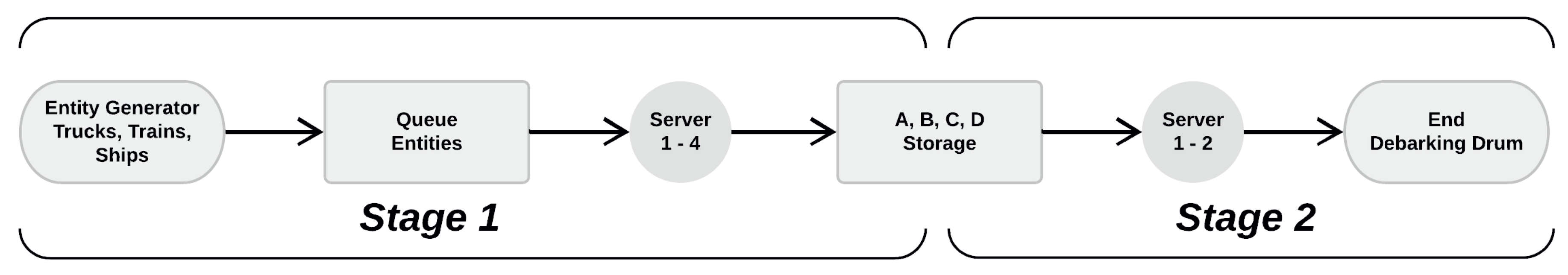
Referring to Figure 2, the general layout of the log-yard process consists of two stages. The first is the arrival of logs at the gate via one of the transport methods: trucks, trains or ships. All these transport methods can arrive independently or simultaneously at any time during the working hours of the day. Vehicles arriving enter a waiting queue for unload by one out of four log-stackers (servers), and the load is placed in a designated storage area within the log-yard. There are four storage areas. In Figure 2, they are labelled as A, B, C and D, and correspond to the storage space for each specific method of transport, i.e., A is for trucks, B is for trains, and C is for ships. An external storage area D works as a buffer for the case when these areas are full.
The second stage of the process consists on feeding the debarking drum with logs coming from any of the four storage areas. To this end, the same log-stacker from stage 1 takes the logs to a debarking drum. The process concludes once the logs enter the debarking drum.
2.1. Data Processing and Normalization
When a truck, train, or ship arrives at the log-yard, the company writes the hour and minute it arrived, and the volume of logs loaded in it. The time is entered in a 24 h format, i.e., 13:30, 14:45, etc. The first step in data processing consists on transforming time, such that all entries in the data have time consecutive, even when days shift. It should also be in a numerical format allowing making mathematical operations. To this end, time is converted into seconds, such that subtracting two consecutive times tells how often entities arrive.
The second step is normalization, which is used to place the data of volume into a similar scale. This step is performed for facilitating the programming of servers, representing the machines working on the log-yard. The difficulty has to do with defining the PDFs formulating the average time it takes to work on an entity. To put it simple, if a truck is unloaded in a given time (usually minutes), and a train is unloaded in time (usually hours), where is much greater than , it is mathematically impractical to create one single probability density function for the unloading time that can take into account this large variation. Similarly, the storage area is programmed as a queue having logs waiting to be fed into the pulp mill. Thus, the time it takes to transport these logs to the pulp mill is somewhat proportional to and . If a machine is used in stage 2, it becomes unavailable to stage 1 and vice-versa. In real life however, stage 1 has the main priority, particularly when trains and ships arrive. Therefore, a machine in stage 2 will interrupt its work when some of these entities arrive at the gate. However, interrupting server work is not something possible in the DEM framework. So, if a server works on an entity, it will do it until it is finished. Thus, it becomes unrealistic to expect that a server will be unavailable a whole time . However, if we consider that / is a proportional value , then it is possible to think that a train is just number of trucks, all arriving simultaneously, i.e., dt = 0. In fact, it is possible to assume that trains and ships are just and number of trucks, thus making trucks the smallest unit of transport to scale the system. After all, they all bring the same objects, i.e., logs, and thus the volume of logs immediately also becomes proportional to one another. A service time , in such a case, becomes also more realistic and removes the idea that the model needs to wait time before it can serve the next entity, either at the gate or storage area. This method of parameterizing a model according to a proportional multiplier is known as normalization and standardization, and it is often done in DEM as a way to develop the mathematics of complex systems involving different entities [22]. Additionally, normalization is a method widely used to facilitate analysis of complex data, and avoid sequences of conditional statements (e.g., if–else commands) in software. Avoiding conditional statements is important to further optimize the system using mathematical optimization.
2.2. Model 1
The reasoning behind model 1 has to do with treating trucks, trains, and ships as different entity forms. Under this concept, each one of them can be given its own PDF, if data show that they follow some forms of these functions. However, the entity generation can only produce a single entity whenever it is time to produce one. Therefore, it is necessary to define an approach, so that the entity generator selects one of these three forms of entities when needed. The selection has to follow similar proportions of these entities as observed in the data. According to data, trucks come in the largest proportion, followed by ships, and last trains (see Figure 4). These procedures are detailed below.
2.3. First Stage
To model the first stage of our system we need four main parameters. These parameters respond to the questions of (1) what is coming (truck, train, or ship), (2) when is it coming (dt), (3) how much volume is it bringing (attribute), and (4) how much time do we need to service it (service time)?
The entities to our first part of the process are the trucks, trains, and ships. The attribute for each entity is the volume of logs they carry in cubic meters (m). The intergeneration time (dt) describes how much time passes between two arriving entities. The service time for the unloading machine depends on the size of the entity, i.e., it takes longer time to unload a train than a truck. The output of this stage is the volume of logs accumulated in areas A, B, C and D. The methods to define each one of these parameters are as follows (Figure 5).
2.3.1. Entity Generation and Attributes
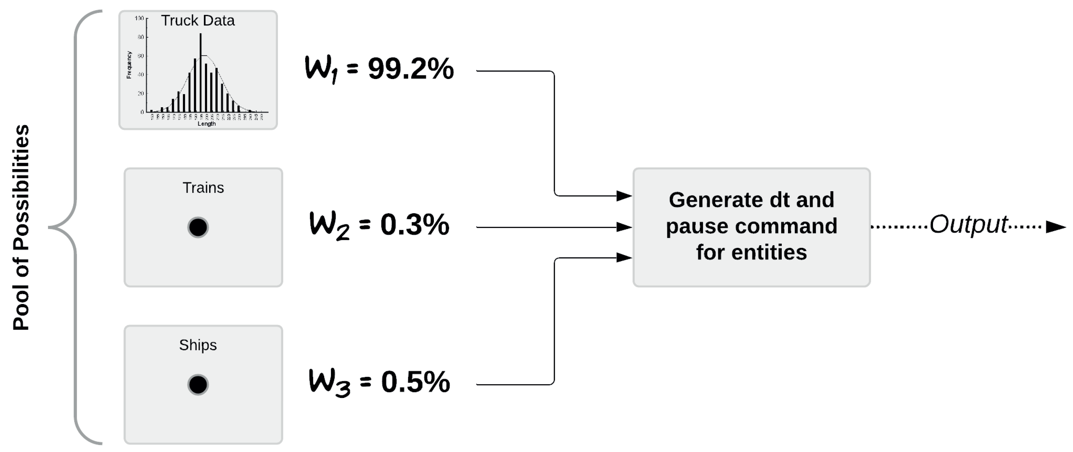
To define entities, we start by considering the case of trucks. One year of company data show that 99.2% of all coming entities correspond to trucks (see Figure 4). For the case of the intergeneration time (dt), these data follow a Generalized Pareto’s PDF:
where is the input value, is the shape parameter, is a scaling parameter and is the threshold parameter (see Table 1).
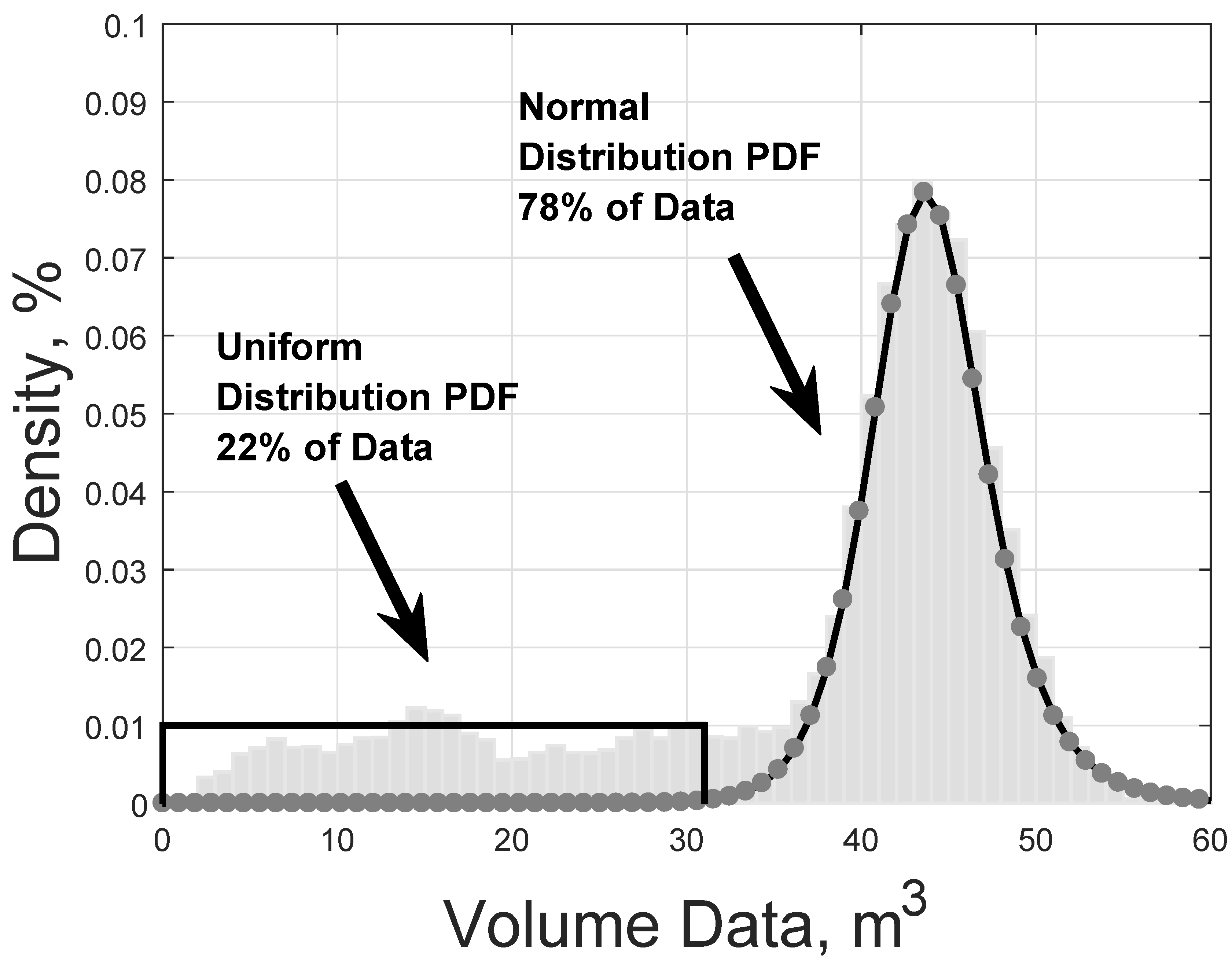
For the case of volume, referring to Figure 6, data show that 22% of the truck volume is distributed from 1 to 30 m following an almost uniform PDF (2c). Above this value, the remaining 78% of data follows a normal PDF (2b). Since these two cases represent two different levels that cannot be captured by a single PDF, our method involves combining them by using a weighted probability density function (2a):
where and are the weights 22% and 78% according to data, and , are the PDFs defined as (2b) and (2c), where and are the input values, is the mean value, is standard deviation, is the lower end point (minimum), is the upper endpoint (maximum) (see Table 1).
The case of trains and ships is using normalized data. To this end, the modelling approach responds to two questions: (1) How often do trains and ships arrive, and (2) What are the values of and to relate them to trucks. According to these questions, one year of data shows that trains and boats arrive three to four times a month, i.e., only once per week, any day of the week. Therefore, in relation to trucks, boats and trains do not follow any deterministic PDF. Hence, they have to be modelled as a random appearance in relation to trucks. As shown in Figure 4, data show that trains come with a frequency of 0.3%, and boats 0.5%.
In terms of mathematical modelling, selecting one of these transport methods corresponds to selecting a number out of a pool of possibilities , where is in the set , corresponding to trucks, trains and ships. This set is allocated with a set of probabilities , such that = in percentage value, and = 100%. If our computer package can return a random integer in the set according to the probability set , then we simply make this value correspond to trucks, trains and ships, having trucks with the highest probability. To define this in software, we can use a uniformly distributed random real number r in the interval (0,1), then the expression
will be a random integer between 1 and 3 according to the probability set . is the cumulative sum of the set , and the inequality is a logical comparison of the random number with C. Once a boat or a train appear during a given week, it is removed from the pool of possibilities through software. In relation to our second question, to define the values for and , the incoming volume of logs in trains and ships in proportion to trucks is taken from the data itself.
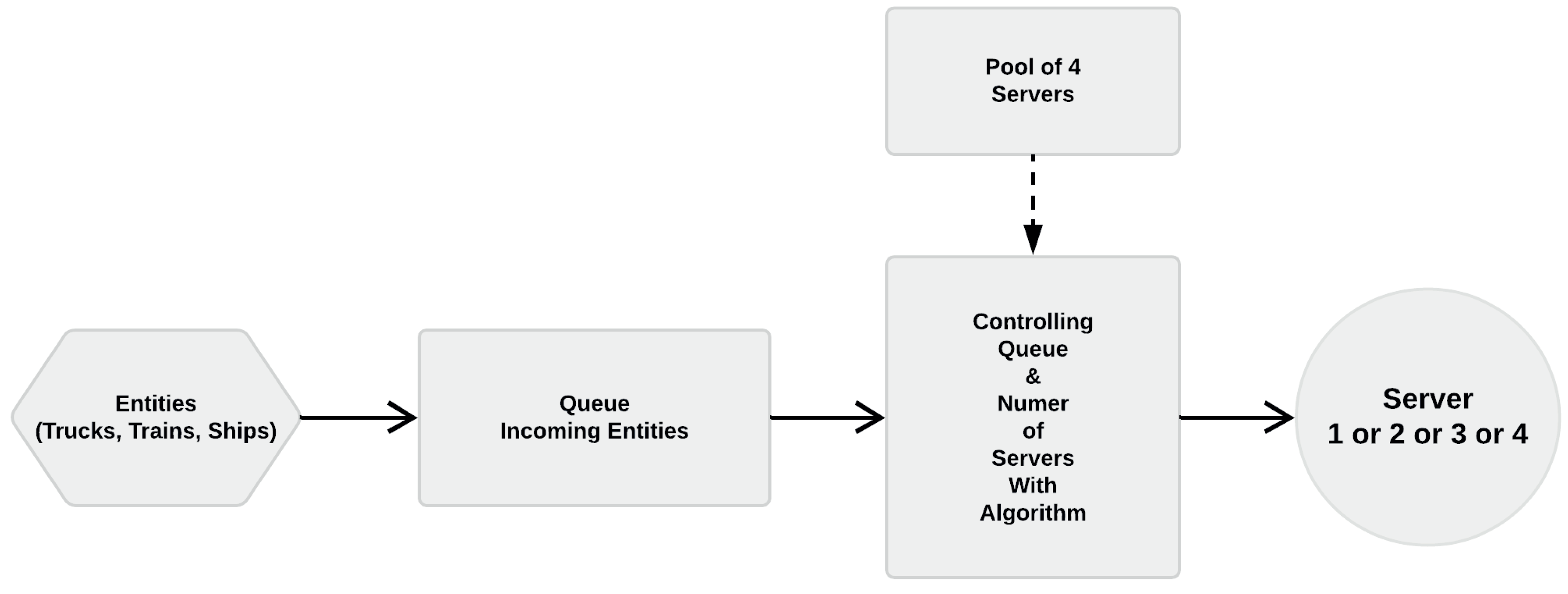
2.3.2. Control over the Size of the Entity Queue and Server Work
A second aspect of our process is the amount of servers (log-stackers) that can work simultaneously at a given moment. To put it simple, if the queue of entities grows because a single server works too slow, then more resources are allocated to keep the system running effectively. In our process, there is a maximum queue length to maintain as an ideal condition, given as a value . As long as the process remains below this value, one single server (log-stacker) is sufficient to provide service to entities. However, when the queue overpasses , more servers are allocated to account for the increasing amount. There is a procedure to increase the amount of servers. This procedure consists on adding servers, once at a time, when the queue reaches specific threshold values. More specifically, when the queue overpasses , then two servers work on the service side. Then, when the queue overpasses , three servers work on the service side. If the queue length overpasses , then all four servers work on the service side. Instead of using conditional if-else coding, the following logic equation gives a mathematical formulation to select the amount of servers:
where q is the number of entities in the queue, and are the values to decide upon the queue length. Figure 7 is a graphical representation of this stage of the process.
Once the amount of servers is defined according to queue length, the next step is to define the service time , referring to the amount of time it takes to unload a given entity. The service time was measured through time studies of work cycles directly at the log-yard. The resulting data show that the server work follows the normal distribution defined as:
where is the input value, is the mean value, is standard deviation (see Table 1).
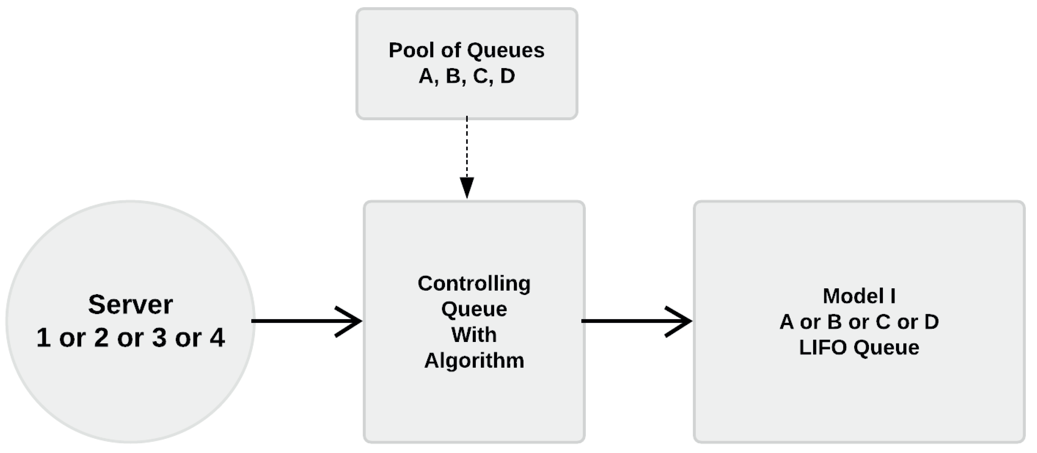
2.3.3. Selecting an Storage Queue for Unload
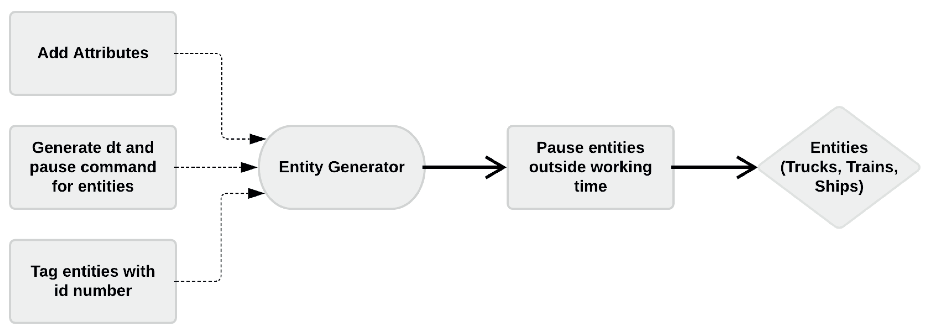
To send logs to the corresponding storage area A, B, C or D, the model needs a way to keep track of the type of entities passing through the process and the amount of entities being queued in each storage area. To this end, an entity id number is created and is attached as part of the entity information once it has been created by the entity generator (Figure 5). The server sends the load to the corresponding area using the id number (Figure 8). However, if the corresponding storage area for trucks, trains and ships has reached its maximum inventory capacity, the load is redirected to the storage area D. The following logic equation gives a mathematical formulation to select the storage area:
where id is the entity type, A, B, C is the storage area and is the maximum inventory capacity for each storage area (see Table 1). The result of will be in the set , representing areas A, B, C, D, correspondingly.
2.4. Second Stage
The second stage follows the principles of the simple example described in Section 1. To begin, the accumulated logs in the storage areas represent the incoming entities to this stage of the model. Then, performing service represents the action of taking these logs to the debarking drum.
2.4.1. Server Work in Stage Two
Usually, the log-stacker in the first stage stacks logs in piles from the bottom up. However, the same machine in the second stage will carry logs from top to bottom. Thus making the system follow a last-in-first-out (LIFO) working method. A second consideration for modelling has to do with the service time for this stage of the process. As explained earlier, when a machine is busy in this second stage, it becomes unavailable to the first stage, and vice versa. However, the first stage has priority, especially when trains or ships arrive in the system. Hence, a machine used in this stage might be interrupted if trucks, trains or ships arrive at the first stage. Interrupting the service time is not something that can be done via DEM. Therefore, the normalization done initially becomes an important mathematical tool to this end. Without normalization, the service time for the volume brought by trains and ships would demand hours of work at the second stage without any possibility to interrupt it during simulation. The PDF for service time would be different for each case (trucks, trains, and ships), and to use them in software would demand conditional statements (e.g., if–else commands), and interrupting them would demand quite extensive and unnecessary programming efforts. Contrary to this, normalization makes the system scaled to the volume of logs in trucks. As result of normalization, the model needs a single PDF to define the service time for this case.
The service time can be formulated with a normal PDF (2b), but using different parameters for and . The service time corresponds to how long it takes to transport logs from these areas to a debarking drum. More specifically, the time it takes to carry logs from the center of the storage area to the debarking drum.
2.4.2. Selecting Logs out of a Storage Area for Log In-Feed to the Mill
One important aspect at the second stage of the process consists on deciding the storage area from which the server will take logs from. According to the process in our study, area A receives the highest priority, followed by C, B and finally D. To this end, our algorithms follow similar procedure described by (3), but with four values to form the set corresponding to areas A, B, C, and D. Then the probability pool is given by = , having = 100%.
2.5. Defining Model Parameters According to Data
So far, we have presented the formulations of PDFs needed to define how the entity intergeneration time and attributes work in our system. However, as observed from (1) to (5) these PDFs contain parameters to define the model behaviour when we perform numerical simulation. The values for these parameters have to be extracted from data.
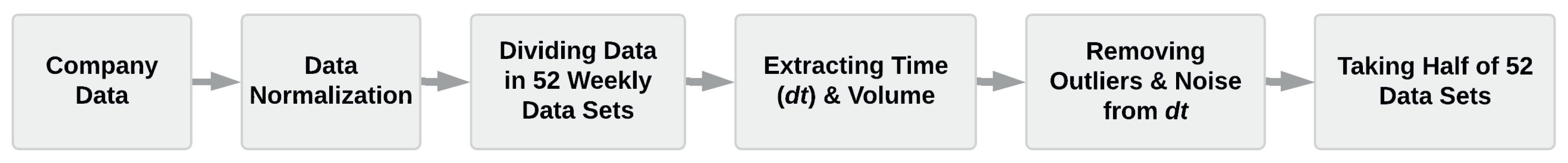
As explained earlier, there are plenty of ways in which data of this kind can be treated. In our particular case, the data are analysed per week, because the company has information of weekly demands. Therefore, one year of data is divided into 52 vectors through software (1 vector for each week). The total data contain 16,131 trucks during one year, with a total volume of 600,000 m. Half of these vectors are used to derive the parameters of the PDFs required for the model. For simplicity, our software uses the first half. Nevertheless, this procedure can be done by selecting half of these vectors in any way, i.e., randomly, or by portions. Using half of the data is done to prevent over-fitting. Over-fitting in data analysis often leads to models that very well capture the behaviour of a data set, but they also learn the noise and outliers, and they becomes unreliable to predict new data sets.
2.5.1. Parameters that Can Be Derived from Data
PDFs functions can be observed by plotting the histogram of the data. Consequently, the method of least-square regression can be used to fit the data to different PDFs (Hayes 2017). In our case, the functions that best fit the data were given from (1) to (2c) and (5). Figure 9 shows the data fitting for the portion of data used for model tuning. The result of the parameters that fit our models given by Equations (1) to (2c) and (5) is given in Table 1.
2.5.2. Parameters that Cannot Be Derived from Data
Mathematically, queue lengths can be infinite because they only represent vectors. In practice, however, the control over the queue lengths have to be done in software by defining vectors of a given size and defining conditions to avoid overflowing them. In our particular case, (4) shows the conditional statements to properly use the four available servers according to a given queue length. The purpose of (4) is to maintain the queue length below the threshold values . Information given by the company sets these values to . However, one of the problems with the process is that despite using all servers at once, it can also happen that the queue size will exceed these numbers, especially when trains or ships arrive in the process. An important performance criterion for the company in this study is raised at this point, because although this happens in reality, it is important to find a working condition in which the ideal situations is maintained, or managed by the process.
The ideal condition of the queue length allows defining parameters for the remaining of the model, for which there are no available data. Some of these parameters define the service time in stage one given by the normal PDF formulated in (5). Nevertheless, these parameters are not set ad-hoc to force the system to behave in a particular way. On the contrary, we have observed the process to extract realistic values by measuring the time it takes to unload trucks. Similarly, all storage areas have restricted capacity, i.e., a maximum inventory capacity (Table 1). The PDF for the service time of stage 2 is determined by the weekly volume demand of 16,000 m of pulpwood from the mill. One server (log-stacker) is assigned to secure that the mill receives the specified volume of logs from all storage areas.
The probability pool defining how often a server in the second stage will visit each storage area is proportional to the storage area’s turnover time. This means that server 2, in model 1, is trying to empty storage areas B and C before next train or ship arrives without causing too much volume accumulation in storage area A and to avoid any inventory build-up in area D. The selection from which storage area the logs should be taken follows (4) according to in Table 1. Once the entity enters the mill, the process concludes.
2.6. Model 2
There are two aspects involved in the reasoning behind model 2. The first has to do with how data are analysed. For model 2, data of trucks, trains, and ships are analysed all together to extract a single PDF for the arrival time and volume. This task is done from the normalized data set. The second factor has to do with the decision-making observed from model 1. Using a single PDF for producing entities removes the necessity to tag an identification number to each entity. Thus, much of the decision-making based upon this number can be removed. Therefore, the system can be modelled as a streamline of stages, as observed in Figure 10.
2.7. Stage 1
2.7.1. Entity Generation
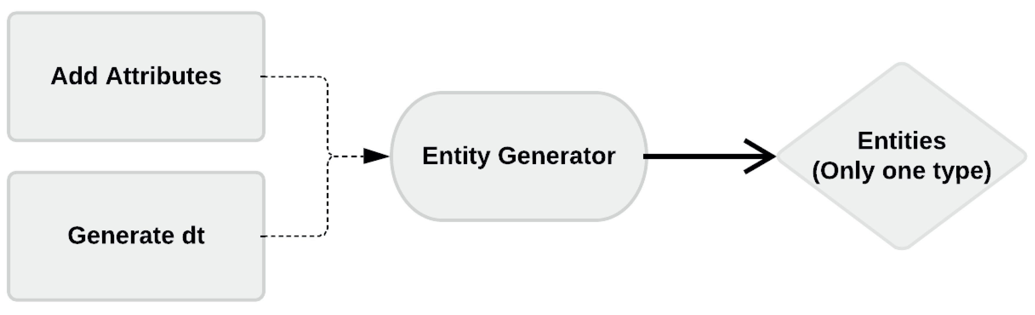
As normalization removes the difference in the data of trucks, trains, and ships, a single PDF is sufficient to represent the dt (Figure 11). To this end, the data are treated per week, similar to what was done for model 1. Because the PDF of dt takes into account the whole week, model 2 can be further simplified by removing pause server after entity generation block compared to model 1. Following this procedure, data fitting suggests that dt follows a weighted combination (7c) of Generalized Pareto’s (7a) and a deterministic uniform PDF (7b) defined as:
where and is the input value, is the shape parameter, is a scaling parameter and is the threshold parameter and is the lower end point (minimum), is the upper endpoint (maximum) and and are the weights between two equations (see Table 2).
Similarly, data show that 17% of the total volume brought by trucks is uniformly spread from one to 30 m. Therefore, the volume follows a Weibull’s PDF for values above 30 m (8a) and a uniform PDF for values below 30 m (8b), weighed by and W (8c).
where and are the input values, is the scale factor and is the shape factor, is the lower end point (minimum), is the upper endpoint (maximum) and and are the weights between two equations (see Table 2).
2.7.2. Entity Queue Control and Server Work
This model uses similar logic as model 1 to control the queue length, and to control the amount of servers providing service to entities.
2.7.3. Storage Queue Selection
Since this model produces only one entity type, it does not take into consideration ID numbers. Thus, it holds only one main storage queue, unlike model 1. Please refer to Figure 12.
2.8. Stage 2
2.8.1. Server Work
2.8.2. Storage Queue Selection for Log in-feed to the Mill
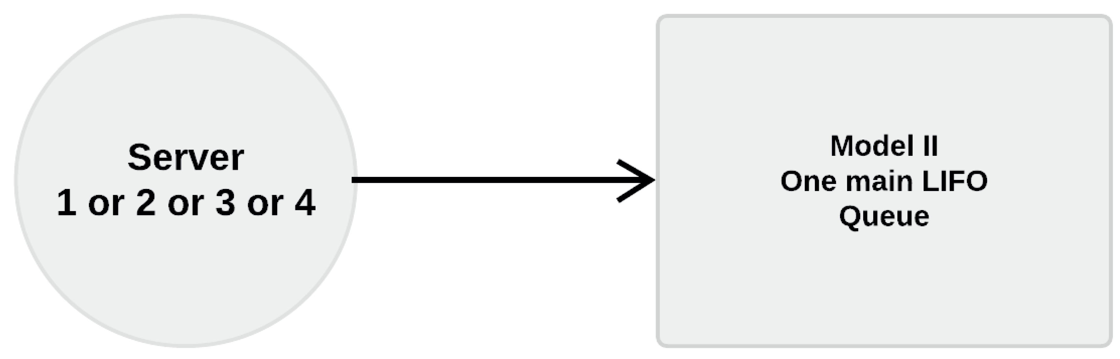
Storage queue selection for log in-feed to the mill is the third main simplification between model 1 and model 2. Since the log-yard represents a storage area, irrespective of whether it has multiple areas or not, then model 2 only has one main storage area representing the log-yard. Therefore, there is no necessity to select the storage area from where to take logs. Thus, all entities can directly enter the server for the mill without extra decision making.
2.8.3. Model Parameter Setting
The procedure to tune this model follows similar principles described for model 1. All parameters required to run simulations with model 2 are summarized in Table 2.
2.9. Method to Draw Quantitative Comparison between Models and Data
Our procedure to perform quantitative comparisons is as follows. Simulation runs are done in the following three cases:
- Case 1: The company data are directly fed into model 1 to record the behaviour of the model according to these data. To this end, the data were organized to provide the necessary intergeneration time, attributes, and id number for each of its entries. After simulation, all the dynamic responses of the data—from stage 1 and 2—were saved.
- Case 2: Model 1 was simulated according to its mathematics presented in Section 2. The simulations are set to produce new values for the PDFs at each run. Thus, each simulation run will be different from the previous. The computer was left to produce 100 simulation results. This process took several hours.
- Case 3: Model 2 was simulated according to its mathematics presented in Section 2. As above, each simulation run is different from the previous. The computer was left to produce 100 simulation results. This process took 1 hour.
Having the results of these three simulation cases, it is possible to draw statistical comparisons. As explained earlier, these models were calibrated according to half of the data. However, the comparison takes place according to the whole data set, to see if the models can predict new data sets. In particular, results of cases 2 and 3 are used to compare against 1.
One initial approach to validate both models in relation to data is by observing the amount of input entities produced in each case, and the output from the very last server in the process. Since the output data are taken from the very last server, the entities at the output are those that the system processed during simulation.
All data analyses, modeling, and simulations were performed using MathWorks’ MATLAB and the Simulink software packages.
3. Results
3.1. Number of Entities for Model 1 and Model 2
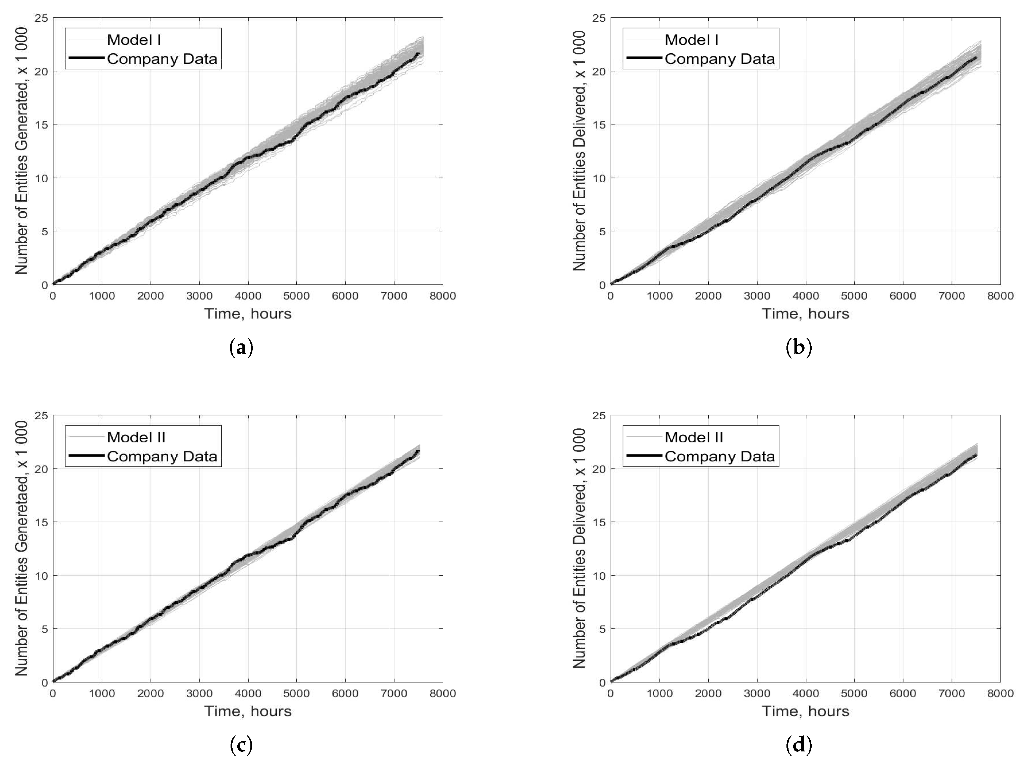
As shown in Table 3, simulations using models 1 and 2 representing one year of the log yard’s operations produced 22,223 and 21,738 entities, respectively, on average. These averages are based on 100 simulation runs each. For comparative purposes, the company’s data show that 21,685 entities arrived over the course of one year. Figure 13a,c show that based on the average of 100 simulation runs, the results obtained with model 1 deviate from the company’s data by 2.5% whereas those obtained with model 2 deviate by only 0.2%.
Figure 13b,d show the output data (i.e., the predicted numbers of delivered entities) for models 1 and 2. The output of model 1 differs from the value indicated by the company data by 2.4%, while that of model 2 differs by 2.7% (Table 3).
Model 1 predicted the generated volume to be 4% higher than the value indicated by the company’s data (877,076 m vs. 844,363 m), while model 2 predicted it to be 0.1% lower (843,545 m) than the value recorded by the company. The models can also be compared based on the volume processed before the output is generated; these values correspond to the final volumes delivered to the mill. Models 1 and 2 predicted the volume delivered to the mill to be 3% and 2% higher, respectively, than the value reported by the company (824,569 m).
3.2. Detailed Results for Model 1
As noted in Section 2.3, model 1 treats deliveries by different modes of transport separately, using concepts of probabilities for deliveries by each mode, whereas model 2 treats them all together and uses a single unified probability density function to determine when deliveries occur. Therefore, it is possible to compare the empirical data on deliveries by different modes to results generated using model 1, but not to those generated using model 2. Model 1 predicts that over the course of an average year, the yard will receive 34 deliveries by ship and 30 deliveries by train, whereas the empirical data show that the yard received 34 deliveries by ship and 24 deliveries by train. The model’s predictions thus deviated from the empirical data by 6% for ships and 22% for trains.
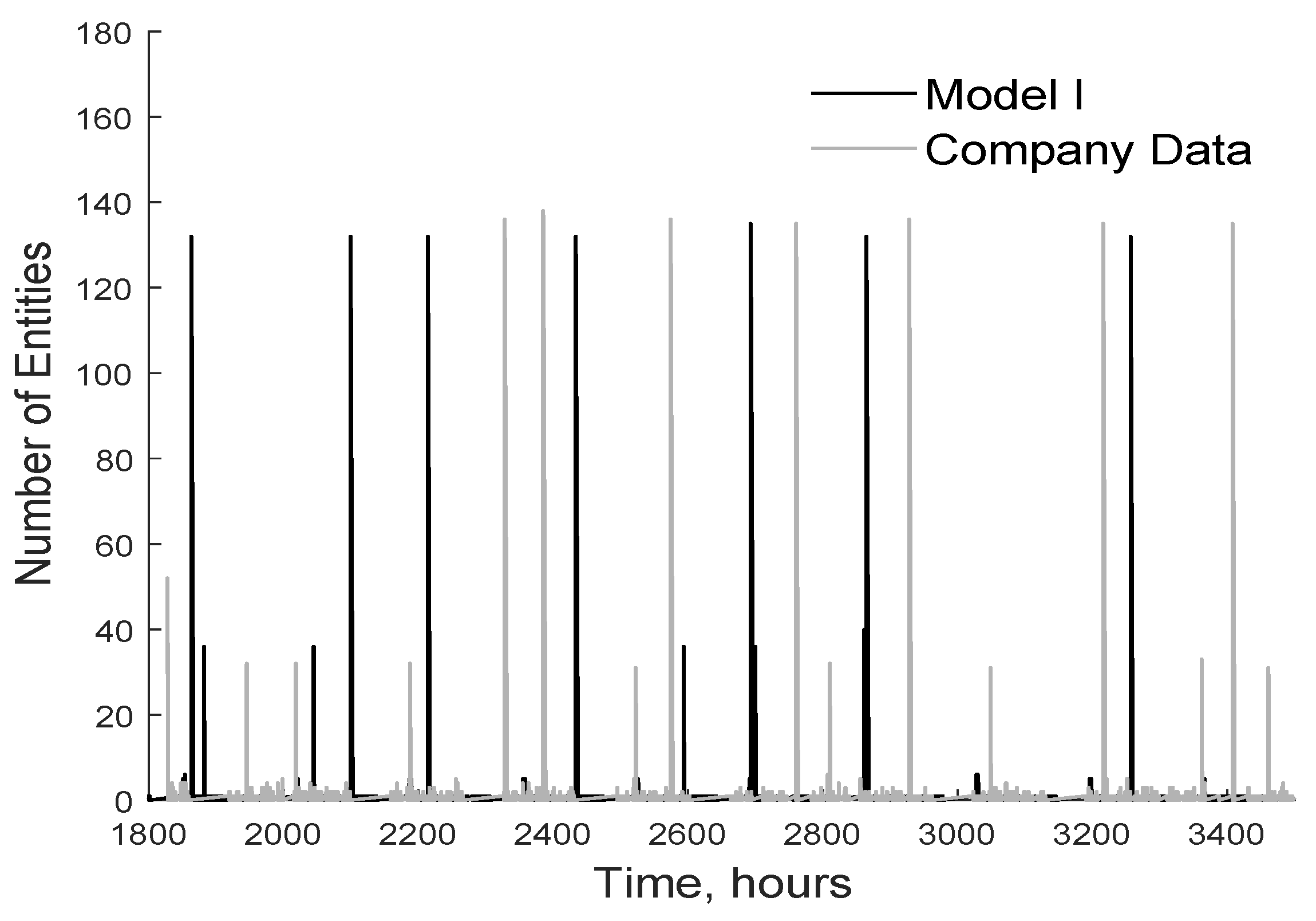
The entities from the entity generator enter a waiting queue, where they remain until they are unloaded. The length of this queue depends strongly on the mode of transport by which the entities were delivered to the yard. In Model 1, the arrival of one ship is represented by the simultaneous arrival of 132 trucks while the arrival of one train is represented by the simultaneous arrival of 36 trucks. Figure 14 shows how the length of the waiting queue varies over the course of a simulation (black line); the peaks correspond to the arrival of a ship or a train at the simulated yard. The corresponding empirical data are also plotted (in grey), showing that the simulation accurately reproduced behavior observed in the real world after normalization.
An important aspect of Model 1 is that the number of working servers depends on the queue size. As explained in Section 2.3.2 and shown in Table 4, the number of working servers may be between one and four. Model 1 predicts that only one server will be active for 71% of the total time. The next most common work pattern occurs when a train or ship arrives at the yard, in which case all four servers must work simultaneously; this occurs 26% of the total time. Situations in which only two or three servers were working accounted for 2.5% and 0.5% of the time, respectively. The company data indicate that one, two, three, and four servers were in operation for 71%, 1.5%, 0.5% and 27% of the total time, respectively.
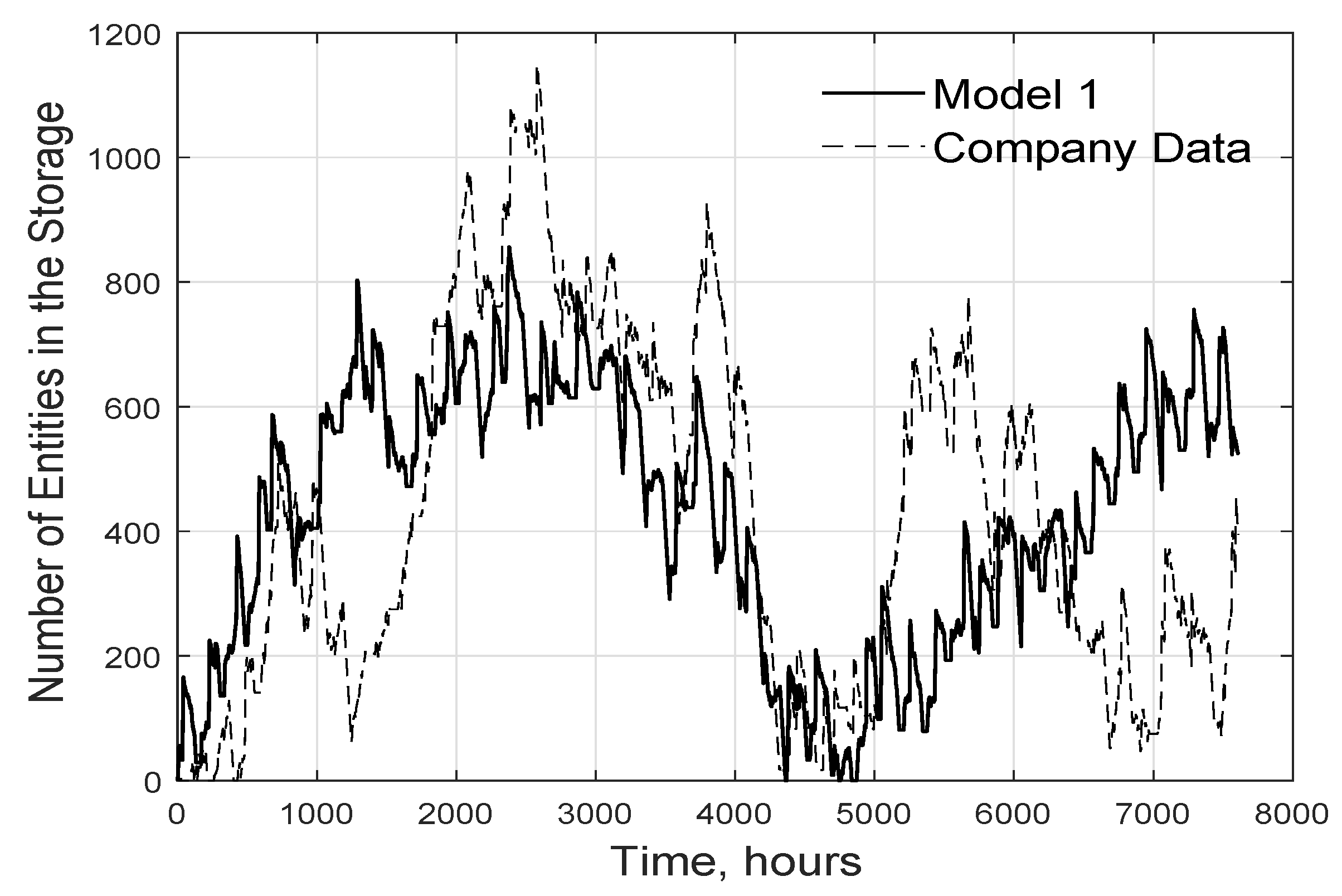
Finally, the numbers of entities in the storage areas were considered. Since each simulation exhibited somewhat different behavior, their results were analyzed at the level of individual runs. As shown in Figure 15, the empirical data indicated that the maximum volume of material in storage was somewhat higher than was predicted by the model. Additionally, the empirical data revealed a number of transient spikes in the stored volume that were not captured in the simulation. Nevertheless, the model’s prediction of the volume in storage at the end of the year agreed quite well with the empirical result, because the model’s internal logic and mathematical approximations were derived from the empirical data.
4. Discussion
Many methods can be used to analytically model complex systems [16,24]. When creating a model with the aim of reproducing real outcomes, data analysis can be a key issue because the way data are treated determines which methods can subsequently be used to model the system. Our objective in this work was to develop a model describing operations at an existing log yard and to verify its ability to reproduce real outcomes by comparing its output to data supplied by the company that manages the yard. To this end, we used two modelling concepts based on different ways of processing and analyzing the available data to illustrate the possibilities offered by mathematics of discrete event modelling. We thus created a hybrid model (model 1) that can be used to study the details of the system’s operations. We also created a purely mathematical model (model 2) that describes the behavior of the system’s main parts. Since model 1 is very detailed, it can be used to show how the existing system behaves in terms of decision making and so on. However, it is not well suited to optimizing or testing alternative scenarios. Model 2 can generate similar results to model 1 but uses strict data normalization and standardization processes as used in statistical modeling, machine learning, and optimization. It can therefore be used to perform numerical optimization in order to find ways of improving process performance, at least within the limitations imposed by the chosen set of PDFs, queues, and servers. By choosing different approaches to data analysis and signal processing, it would be possible to implement many other modeling strategies representing intermediates between the two extremes presented here.
A major challenge in data analysis is to extract valuable information from a potentially large quantity of data. A significant problem during this work was that the data supplied by the company only covered its operations over one year; a dataset covering a longer period, such as six years, would have enabled analysis of year-on-year variation in the log yard’s operating processes. Since no such data were available, the models presented here can be considered reliable for the year covered by the data, but we cannot say with certainty that this is sufficient to describe the performance of the company’s processes over longer periods. However, if we assume that there are no large variations in the way the company operates, our models should provide reliable estimates for longer periods.
When using company data, it can be challenging to create PDFs that accurately reflect real-world outcomes because the behavior of real systems is not always well described by standard PDFs. Our results show that the behavior of real systems can sometimes be approximated using weighted PDFs in such cases. Although weighted PDFs are rarely used in discrete event modeling, they are widely used with other modeling methods. The problem with this approach is that the results obtained become highly targeted to the data set on which the PDFs are based. Consequently, the validity of the approximation in contexts outside that represented by the available data is questionable unless there is reason to believe that there is no appreciable long-term variation in the studied process and/or operations. This is another reason why it would be desirable to have a dataset covering a longer period of time. The use of weighted PDFs is exemplified by the treatment of the variable input entities, i.e., trains, ships, and trucks. In model 1, each mode of transport is analyzed separately and their arrivals are coordinated using probability theory. In model 2, all methods of transport are described using a single PDF, which have to be weighted to achieve reasonable agreement with the company’s data. A similar situation occurs when dealing with data that vary over a wide range, as was the case when adapting the model to account for the possibility of partial deliveries (i.e., deliveries in which the yard receives only a fraction of the volume carried by a train, truck, or ship). Full deliveries could be modeled well using a normal or Weibull PDF. However, low-volume deliveries (partial truck loads) accounted for too large a share of the total delivered volume to be ignored but were not well described by any PDFs that could also describe full deliveries. Therefore, a weighted PDF was used to model the combined occurrence of full and partial deliveries (the latter being defined as deliveries of up to 30 m). An alternative to using weighted PDFs in such cases is to use two-dimensional cluster functions, which are used extensively in principal component analysis [25]. Cluster functions can give almost 0% error in data fitting [26,27]. However, they are more difficult to use in the context of modelling, and overfitting data does not necessarily result in more accurate simulations.
After running 100 simulation trials each representing one year of the log yard’s operations, the average values for the input and output entities obtained using both models were within 3% of the value indicated by the company’s data. It was not necessary to perform multiple simulations to estimate the confidence intervals for the models’ predictions because their values are embedded in the PDFs and could thus be calculated analytically. The models’ predictive accuracy is very good given that they were calibrated using only half the available data but tested against the complete company data set. However, although the input and output values agree well with the empirical data, there is no way to verify that the models’ descriptions of the yard’s internal operations agree well with reality due to a lack of suitable reference data. This limits the reliability of our results.
A challenging issue for any model is to capture dynamics over the entire simulated period. Figure 13a,c show the predictions of models 1 and 2 agree well with the company data between 0 and ca. 3500 h, but the models fail to capture a fall in the number of arriving entities between 3500 and ca. 5300 h. A similar pattern exists in Figure 13b,d, where both models closely follow the company data until ca. 1200 h but fail to capture a slight fall thereafter. In both cases, the fall in the number of arriving entities observed in the company data could be due to vacation time or holidays. No effort was made to model vacations and holidays because doing so was expected to require considerable programming effort without greatly improving the models’ predictive accuracy.
As noted previously, each of the two models presented here has distinct strengths and limitations. The strength of model 2 is its mathematical simplicity and its ability to describe the yard’s operations as a linear sequence of events with very few decision-making stages. Conversely, the strength of model 1 is its ability to shed light on the details of the yard’s processes and operations, at the cost of requiring many conditional statements to describe decision-making. Unfortunately, conditional statements give rise to bifurcations in simulations, making mathematical optimization difficult or impossible. Model 2 is thus better suited for optimization purposes because it uses analytical expressions in place of many of the conditional statements used in model 1.
Data representing real life operations often cannot be described using a single PDF, so a combination of PDFs may be needed to obtain an accurate description. The results presented here show that using DEM in conjunction with two different approaches to data analysis enabled reliable prediction of the studied log yard’s inputs and outputs. The two models presented here have different strengths: model 2 is the most appropriate if seeking to estimate the number of entities handled at the yard per year and for performing optimization, while model 1 is best for characterizing the flow of material through the yard and identifying bottlenecks.
Author Contributions
Conceptualization, K.K., P.L.H. and D.B.; methodology, P.L.H. and K.K.; software, K.K. and P.L.H.; validation, K.K. and P.L.H.; formal analysis, K.K.; investigation, K.K.; resources, D.B. and P.L.H.; data curation, K.K. and P.L.H.; writing—original draft preparation, K.K., P.L.H. and D.B.; writing—review and editing, K.K., P.L.H. and D.B.; visualization, K.K. and P.L.H.; supervision, D.B. and P.L.H.; project administration, D.B.; funding acquisition, D.B. All authors have read and agreed to the published version of the manuscript.
Funding
This research was part of the BioHub project financed by the Botnia-Atlantica program, under the European Regional Development Fund.
Acknowledgments
The authors gratefully acknowledge the help of Domsjö Fiber AB for providing data regarding log-yard operations.
Conflicts of Interest
The authors declare no conflict of interest and the funders had no role in the design of the study; in the collection, analyses, or interpretation of data; in the writing of the manuscript, or in the decision to publish the results.
References
- Berg, M.; Kinnwall, M.; Heinsoo, K.; Niklasson, M. Så går det för skogsindustrin [This Is How It Is Going for Forest Industry]; Report 1; Skogsindustrierna: Stockholm, Sweden, 2018. [Google Scholar]
- Asikainen, A. Simulation of Logging and Barge Transport of Wood from Forests on Islands. Int. J. For. Eng. 2001, 12, 43–50. [Google Scholar] [CrossRef] [Green Version]
- Karttunen, K.; Lättilä, L.; Korpinen, O.J.; Ranta, T. Cost-efficiency of intermodal container supply chain for forest chips. Silva Fennica 2013, 47, 24. [Google Scholar] [CrossRef] [Green Version]
- Väätäinen, K.; Prinz, R.; Malinen, J.; Laitila, J.; Sikanen, L. Alternative operation models for using a feed-in terminal as a part of the forest chip supply system for a CHP plant. Gcb Bioenergy 2017, 9, 1657–1673. [Google Scholar] [CrossRef] [Green Version]
- Arriagada, R.A.; Cubbage, F.W.; Abt, K.L.; Huggett, R.J., Jr. Estimating harvest costs for fuel treatments in the West. For. Prod. J. 2008, 58, 24. [Google Scholar]
- Eriksson, A.; Eliasson, L.; Jirjis, R. Simulation-based evaluation of supply chains for stump fuel. Int. J. For. Eng. 2014, 1–14. [Google Scholar] [CrossRef]
- Berg, S.; Bergström, D.; Nordfjell, T. Simulating conventional and integrated stump- and round-wood harvesting systems: A comparison of productivity and costs. Int. J. For. Eng. 2014, 25, 138–155. [Google Scholar] [CrossRef]
- Pinho, T.M.; Coelho, J.P.; Moreira, A.P.; Boaventura-Cunha, J. Modelling a biomass supply chain through discrete-event simulation. IFAC-PapersOnLine 2016, 49, 84–89. [Google Scholar] [CrossRef]
- Chiorescu, S.; Gronlund, A. Assessing the role of the harvester within the forestry-wood chain. For. Prod. J. 2001, 51, 77. [Google Scholar]
- Salichon, M.C. Simulating Changing Diameter Distributions in a Softwood Sawmill. Master’s Thesis, Graduate School, Oregon State University, Corvallis, OR, USA, 2005. [Google Scholar]
- Mendoza, G.A.; Meimban, R.J.; Araman, P.A.; Luppold, W.G. Combined log inventory and process simulation models for the planning and control of sawmill operations. In Proceedings of the 23rd CIRP International Seminar on Manufacturing Systems, Nancy, France, 6–7 June 1991; p. 8. [Google Scholar]
- Rahman, A.; Yella, S.; Dougherty, M. Simulation model using meta heuristic algorithms for achieving optimal arrangement of storage bins in a sawmill yard. J. Intell. Learn. Syst. Appl. 2014, 6, 125–139. [Google Scholar] [CrossRef] [Green Version]
- Beaudoin, D.; LeBel, L.; Soussi, M.A. Discrete Event Simulation to Improve Log Yard Operations. INFOR Inf. Syst. Oper. Res. 2013, 50, 175–185. [Google Scholar] [CrossRef] [Green Version]
- Puodziunas, M.; Fjeld, D. Roundwood Handling at a Lithuanian Sawmill-Discrete-event Simulation of Sourcing and Delivery Scheduling. Baltic For. 2008, 14, 163–175. [Google Scholar]
- LeBel, L.; Carruth, J.S. Simulation of woodyard inventory variations using a stochastic model. For. Prod. J. 1997, 47, 52. [Google Scholar]
- Taha, H.A. Operations Research: An Introduction, 5th ed.; Macmillan: Detroit, MI, USA, 1992; Volume 1. [Google Scholar]
- Lättilä, L. Improving Transportation and Warehousing Efficiency with Simulation-Based Decision Support Systems. Ph.D. Thesis, Faculty of Technology Management, Industrial Management, Lappeenranta University of Technology, Lappeenranta, Finland, 2012. [Google Scholar]
- Aalto, M.; Raghu, K.C.; Korpinen, O.J.; Karttunen, K.; Ranta, T. Modeling of biomass supply system by combining computational methods—A review article. Appl. Energy 2019, 243, 145–154. [Google Scholar] [CrossRef]
- Zeigler, B.P.; Kim, T.G.; Praehofer, H. Theory of Modeling and Simulation, 2nd ed.; Academic Press, Elsevier: London, UK, 2000. [Google Scholar]
- Silverman, B.W. Density Estimation for Statistics and Data Analysis; Chapman & Hall/CRC: London, UK, 2018. [Google Scholar]
- Väätäinen, K.; Asikainen, A.; Eronen, J. Improving the Logistics of Biofuel Reception at the Power Plant of Kuopio City. Int. J. For. Eng. 2005, 16, 51–64. [Google Scholar] [CrossRef]
- Laguna, M.; Marti, R. Neural network prediction in a system for optimizing simulations. Iie Trans. 2002, 34, 273–282. [Google Scholar] [CrossRef]
- Ljung, L. System Identification. In Wiley Encyclopedia of Electrical and Electronics Engineering; John Wiley & Sons: Hoboken, NJ, USA, 2017; pp. 1–19. [Google Scholar] [CrossRef]
- Robinson, S. Simulation: The Practice of Model Development and Use; John Willey and Sons: Chichester, UK, 2004; Volume 1, p. 5. [Google Scholar]
- Jain, A.K.; Murty, M.N.; Flynn, P.J. Data clustering: A review. ACM Comput. Surv. (CSUR) 1999, 31, 264–323. [Google Scholar] [CrossRef]
- Krishnapuram, R.; Freg, C.P. Fitting an unknown number of lines and planes to image data through compatible cluster merging. Patt. Recogn. 1992, 25, 385–400. [Google Scholar] [CrossRef]
- Setnes, M.; Babuska, R.; Verbruggen, H.B. Rule-based modeling: Precision and transparency. IEEE Trans. Syst. Man Cybernet. Part C (Appl. Rev.) 1998, 28, 165–169. [Google Scholar] [CrossRef] [Green Version]
Figure 1.
Flowchart depicting the flow and the main components of a discrete event model.

Figure 2.
A general model 1 system layout of log-yard logistics at a pulp mill.

Figure 3.
Data processing steps.

Figure 4.
Layout representing three different transport methods, going into an algorithm to produce a single entity out of them.
Figure 4.
Layout representing three different transport methods, going into an algorithm to produce a single entity out of them.

Figure 5.
After an entity has been selected (see Figure 4), the remaining of the operation is to define its attribute (volume of logs), and an id tag to differentiate them throughout the simulation process.
Figure 5.
After an entity has been selected (see Figure 4), the remaining of the operation is to define its attribute (volume of logs), and an id tag to differentiate them throughout the simulation process.

Figure 6.
Histogram showing the amount of volume for trucks.

Figure 7.
Block scheme of controlling queue length of incoming entities and number of working servers.
Figure 7.
Block scheme of controlling queue length of incoming entities and number of working servers.

Figure 8.
Block scheme of controlling entity path to the right queue in the storage area.

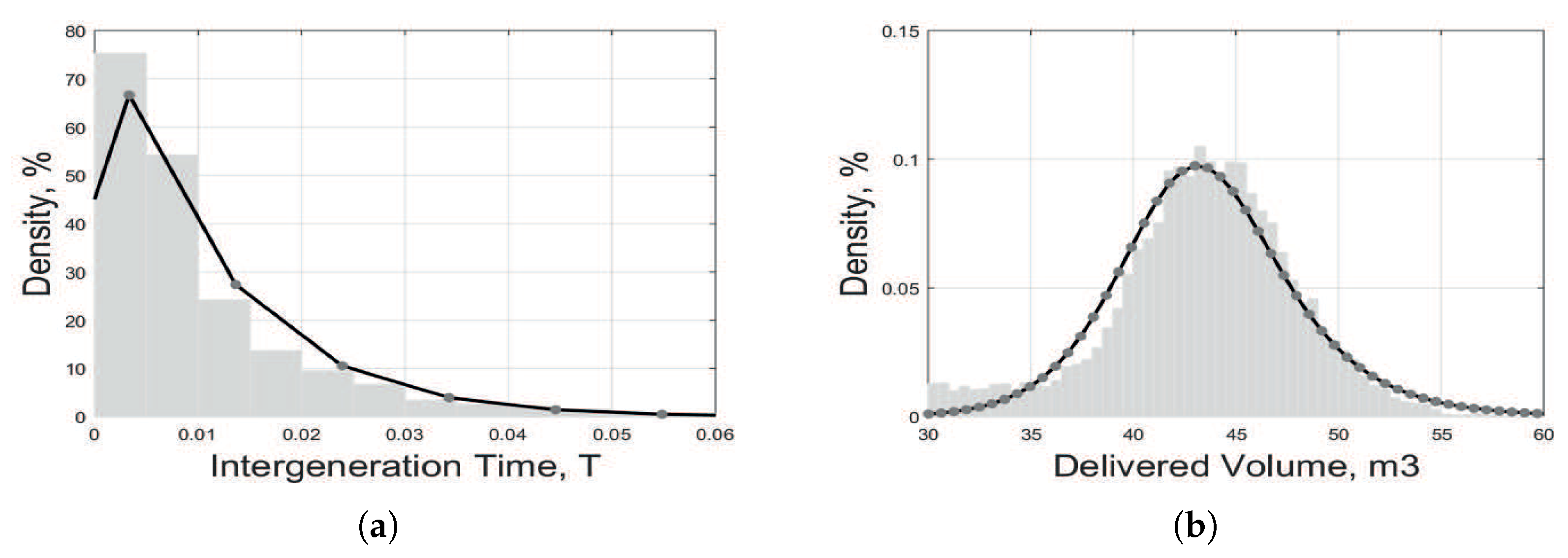
Figure 9.
Data fitting of intergeneration time (a) and attribute for delivered log volume (b). Where the grey area is a empirical data from company and bold line is showing fitting of the PDF.
Figure 9.
Data fitting of intergeneration time (a) and attribute for delivered log volume (b). Where the grey area is a empirical data from company and bold line is showing fitting of the PDF.

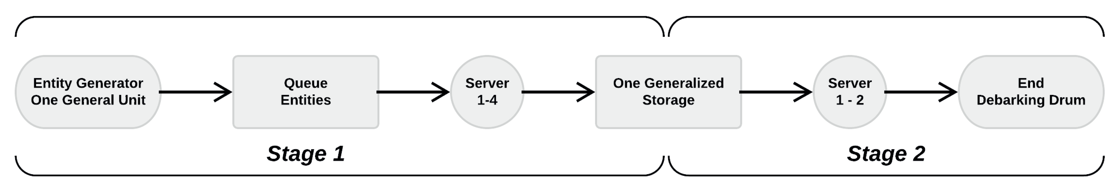
Figure 10.
A general model 2 system layout of log-yard logistics at a pulp mill.

Figure 11.
Entity generator block diagram for model 2.

Figure 12.
Block scheme of entities path to the main storage area in model 2.

Figure 13.
Total numbers of generated and delivered entities based 100 simulation runs representing one year of the log yard’s operations using Model 1 (a,b) and Model 2 (c,d).
Figure 13.
Total numbers of generated and delivered entities based 100 simulation runs representing one year of the log yard’s operations using Model 1 (a,b) and Model 2 (c,d).

Figure 14.
Number of waiting entities to be unloaded at Stage 1. The dark solid line represents results obtained using Model 1, while the grey line shows company data.
Figure 14.
Number of waiting entities to be unloaded at Stage 1. The dark solid line represents results obtained using Model 1, while the grey line shows company data.

Figure 15.
One example result of total inventory level of entities as predicted by model 1 and indicated by the company data.
Figure 15.
One example result of total inventory level of entities as predicted by model 1 and indicated by the company data.


Table 1.
Model 1 parameters.
| Parameter | Value |
|---|---|
| Solver | Fixed Step Discrete |
| Fixed Step Size (fundamental sample time), s | 300 |
| Model 1 Total Simulated Time, s | 2.7388 |
| 36 | |
| 132 | |
| 0.3680 | |
| 0.0078 | |
| 0.00361 | |
| , m | 45.4302 |
| , m | 4.5819 |
| , m | 1 |
| , m | 30 |
| 0.78 | |
| 0.22 | |
| , entities | 3 |
| , entities | 5 |
| , entities | >7 |
| , sec | 319 |
| , sec | 75 |
| , sec | 832.9049 |
| , sec | 249.8715 |
| , Storage A, m | 40,000 |
| , Storage B, m | 15,000 |
| , Storage C, m | 7000 |
| , Storage D, m | ∞ |
| , % | 99.2 |
| , % | 0.3 |
| , % | 0.5 |
| , % | 55 |
| , % | 8 |
| , % | 35 |
| , % | 2 |
Table 2.
Model 2 parameters.
| Parameter | Value |
|---|---|
| Solver | Fixed Step Discrete |
| Fixed Step Size (fundamental sample time), s | 300 |
| Total Model 2 Simulation Time, s | 1.8576 |
| 36 | |
| 132 | |
| 0.4243 | |
| 0.0076 | |
| 0.002 | |
| , m | 45.9942 |
| , m | 9.65723 |
| , m | 1 |
| , m | 30 |
| 0 | |
| 0.0007 | |
| 0.83 | |
| 0.17 | |
| 0.64 | |
| 0.36 | |
| , entities | 3 |
| , entities | 5 |
| , entities | >7 |
| , sec | 319 |
| , sec | 75 |
| , sec | 564.8994 |
| , sec | 169.4698 |
| Main Storage, m | >62,000 |
Table 3.
Total number of generated and delivered entities over one year period based on 100 simulation runs using models 1 and 2. * Confidence intervals based on the final values of the simulations.
Table 3.
Total number of generated and delivered entities over one year period based on 100 simulation runs using models 1 and 2. * Confidence intervals based on the final values of the simulations.
| Difference from Company Data, % | Standard Deviation | Standard Error | T-Score | Confidence Interval 5% * | ||||
|---|---|---|---|---|---|---|---|---|
| Lower | Upper | Lower | Upper | |||||
| Generated Entities (INPUT) | ||||||||
| Model 1 | 22,223 | 2.5 | 6332 | 42.4828 | −1.9601 | 1.9601 | 22,138 | 22,307 |
| Model 2 | 21,738 | 0.2 | 6230 | 42.2557 | −1.9601 | 1.9601 | 21,654 | 21,822 |
| Company Data | 21,685 | - | - | - | - | - | - | - |
| Delivered Entities (OUTPUT) | ||||||||
| Model 1 | 21,666 | 2.4 | 6216 | 42.2336 | −1.9601 | 1.9601 | 21,583 | 21,750 |
| Model 2 | 21,742 | 2.7 | 6323 | 42.9702 | −1.9601 | 1.9601 | 21,659 | 21,825 |
| Company Data | 21,167 | - | - | - | - | - | - | - |
Table 4.
Proportion of entities unloaded while different numbers of servers were operating.
| Percentage of Unloaded Entities per Server Combination | ||||
|---|---|---|---|---|
| 1 Server | 2 Servers | 3 Servers | 4 Servers | |
| Model 1 | 71.0 | 2.5 | 0.5 | 26.0 |
| Company Data | 71.0 | 1.5 | 0.5 | 27.0 |
© 2020 by the authors. Licensee MDPI, Basel, Switzerland. This article is an open access article distributed under the terms and conditions of the Creative Commons Attribution (CC BY) license (http://creativecommons.org/licenses/by/4.0/).
Share and Cite
MDPI and ACS Style
Kons, K.; La Hera, P.; Bergström, D. Modelling Dynamics of a Log-Yard through Discrete-Event Mathematics. Forests 2020, 11, 155. https://doi.org/10.3390/f11020155
AMA Style
Kons K, La Hera P, Bergström D. Modelling Dynamics of a Log-Yard through Discrete-Event Mathematics. Forests. 2020; 11(2):155. https://doi.org/10.3390/f11020155
Chicago/Turabian StyleKons, Kalvis, Pedro La Hera, and Dan Bergström. 2020. "Modelling Dynamics of a Log-Yard through Discrete-Event Mathematics" Forests 11, no. 2: 155. https://doi.org/10.3390/f11020155
Note that from the first issue of 2016, this journal uses article numbers instead of page numbers. See further details here.